


Abstract
The Samara River is a left-bank tributary of the Volga with a total basin area of 46,500 km2, of which 22,800 km2 is the gauged area analyzed in this study. This river system serves as a case study for examining hydrological transformations in the extreme southeastern region of European Russia (the Southern Cis-Urals) driven by progressive climate change and historical land-use shifts. To achieve this, the study analyzes long-term, station-based gauge observations of monthly river runoff for the period 1933–2022. The methodology employs a baseline set of standard statistical criteria combined with specialized hydromathematical procedures to evaluate runoff structure. The results demonstrate that while the river’s annual runoff lacked a statistically significant trend, its intra-annual structure underwent profound transformations. While April and May exhibited non-significant declines, the vast majority of months demonstrated prominent upward runoff trends. This systematic increase compressed the amplitude between hydrologically contrasting months by a factor of 2.5 to 3 from the historical climatological baseline (1933–1960) period to the modern baseline (1991–2020) period. Since 1989, the intra-annual variability coefficient has decreased by approximately one-third, especially during low-flow years. Concurrently, the spring flood contribution decreased by approximately 25%, and the frequency of prolonged, three- to four-month snowmelt-driven freshets during the 1987–2022 period doubled to ~22% compared to the preceding period, whereas the summer–autumn and winter low-flow shares increased substantially. Spectral analysis demonstrates a structural asymmetry in runoff generation mechanisms: low-flow dynamics are predominantly governed by long-term macrocycles (spanning 11 years or more), whereas maximum discharge exhibits a complex spectral configuration rather than a purely stochastic white noise process, reflecting an underlying statistical ambiguity between the applied criteria. Finally, five alternating multiyear flow phases occurred since 1933, characterized by low-flow conditions during 1933–1945, 1966–1984, and 2014–2022, and high-flow conditions during 1946–1965 and 1985–2013, with the respective contributions of the spring snowmelt flood and low-flow runoff differing substantially across these phases. This research advances the understanding of regional river runoff transformations in the Anthropocene, providing an objective basis for long-term water balance forecasting in the Southern Cis-Urals, strategic environmental management, climate change adaptation, and environmental risk assessment.
1. Introduction
Global climate change drives profound and often nonlinear alterations across planetary systems, resulting in shifts that appear particularly amplified in northern high latitudes, including the Russian Federation [1]. These shifting hydroclimatic regimes directly affect surface waters, compromising river runoff stability, regional water security, and the long-term dynamics of aquatic and riparian ecosystems [2]. Across Europe, and specifically the East European Plain, contemporary climate variations [1,3,4,5,6,7] have closely coincided with sweeping land-use and land-cover changes (LULCC) [8,9,10,11,12,13]. In Russia, particularly within its European sector, these anthropogenic transformations accelerated following the socioeconomic transitions of the late 1980s and early 1990s. This period was characterized by a widespread abandonment of arable land—most manifest in the southern forest zone and, to a lesser extent, within the forest-steppe and steppe landscape zones—alongside major structural shifts in crop rotation cycles and agricultural machinery utilization.
These dual drivers—hydroclimatic shifts and rapid LULCC—increasingly converge within the conceptual framework of the Anthropocene. This proposed geological epoch highlights an era of unprecedented human dominance over Earth’s planetary systems, a trajectory that became explicitly evident during the “Great Acceleration” of the mid-20th century [14,15,16,17]. Globally demarcated by the intensive atmospheric nuclear weapons testing of the 1950s and 1960s [18,19,20], this anthropogenic legacy left a permanent, long-term stratigraphic marker. Although awaiting formal IUGS ratification, the Anthropocene provides an essential baseline for assessing how riverine networks respond to cumulative pressures [21,22,23,24,25,26,27]. While large-scale hydrological shifts are frequently documented for continental-scale basins, the complex, localized, and potentially more vulnerable responses of small and medium-sized river systems to these combined Anthropocene pressures remain disproportionately understudied.
The overarching trends governing runoff transformation, including variations in multiyear annual means and general intra-annual distribution patterns, have been progressively characterized at the macroregional scale across the entire East European Plain, with a particular focus on its southern sector [28,29,30,31,32,33,34,35,36,37,38,39]. Notably, these regional patterns closely align with broader subcontinental dynamics, where widespread climate-driven shifts in flood timing and volumes have been extensively observed across both Western and Eastern Europe [40,41,42,43,44]. Prior studies demonstrate that rising winter air temperatures and, consequently, more frequent winter thaws in recent decades have driven a substantial increase in the winter baseflow of plain rivers [29,30,31,37]. Concurrently, spring snowmelt floods—historically the dominant hydrological phase for these continental drainage basins—have exhibited a marked decline in both volume and peak intensity [28,29,30,41], especially across the southern margins of the plain. These transformations in spring freshets are primarily attributed to reduced winter snow accumulation immediately prior to the onset of snowmelt (driven by winter thaws and enhanced sublimation from the snowpack surface under warming winter and spring air temperatures) alongside decreasing soil freezing depths, which facilitate more intensive infiltration of meltwater into groundwater storage. These hydroclimatic response pathways varied slightly across different regions of the plain, modulated by local geological, geomorphological, and landscape characteristics.
Despite these regional insights, a critical knowledge gap persists within contemporary hydrology. The overwhelming majority of the extant literature relies on isolated, univariate trend detection frameworks applied to single variables, thereby generating a profound deficit of comprehensive, multidimensional diagnostic approaches. Specifically, there is a distinct lack of integrated methodologies capable of simultaneously evaluating long-term monotonic trends, periodic cyclicities, discrete multiyear high- and low-flow regimes, and the structural reconfigurations of distinct seasonal hydrological phases under Anthropocene pressures. Furthermore, such comprehensive Anthropocene runoff transformations remain critically underinvestigated within the Southern Cis-Urals region—a hydroclimatically sensitive transition zone between forest-steppe and steppe landscapes situated at the intersection of the East European Plain and the Ural Mountains.
To address this gap, this study examines the long-term, comprehensive hydrological transformations within the Southern Cis-Urals, utilizing the Samara River—a medium-sized river that serves as a highly representative hydrological proxy for the region. Unlike other major rivers in the macro-region, such as the Ural and Belaya, which originate in the Ural Mountains—a region characterized by landscapes transitioning from steppes to forests—and thus function as transregional, transit watercourses, the Samara River basin is situated entirely within lowland and upland forest-steppe and steppe ecozones, which are highly characteristic of the Southern Cis-Urals proper. Consequently, its hydrological regime perfectly reflects the climate-driven vulnerabilities intrinsic to the macroregion, characterized by an absolute dependence on snowmelt-driven spring freshets and pronounced summer–autumn low-flow seasons. The distinct scientific value of this research lies in its extensive retrospective analysis, which leverages a continuous, high-quality empirical dataset of gauge-based observations spanning 1933–2022. Such an extensive 90-year dataset remains exceedingly rare in both global and regional hydrological research, enabling the systematic verification of regional hydroclimatic shifts prior to and during the “Great Acceleration.”
2. Materials and Methods
2.1. The Samara River and Its Basin
This study focuses on the Samara River (source: 52°03′09″ N, 54°33′39″ E), a major left-bank tributary of the Volga—Europe’s largest river. Stretching 594 km with a drainage basin encompassing 46,500 km2, the river originates on the southeastern slopes of the Obshchy Syrt Upland (Figure 1). The upland features prevailing elevations of 200–300 m a.s.l., which increase to 350–400 m eastward within the eastern sector of the basin. In the lower course, the river traverses the Trans-Volga Lowland, which is characterized by dominant elevations of 50–150 m that decline to 28–32 m at the water line within the main valleys. In its upper course, the river emerges as a narrow steppe creek before gradually widening. The river valley is asymmetric, featuring a steep right bank and a gentle left bank. The width of the valley expands to 10–16 km within the middle and lower reaches. The Samara River is fed by more than 200 tributaries and small streams.
Figure 1.
Location of the Samara River within the eastern East European Plain. 1—main orographic units of the study region (OSU—Obshchy Syrt Upland; BBU—Bugulma–Belebey Upland; TVL—Trans-Volga Lowland); 2—river network; 3—analyzed gauging station on the Samara River near Yelshanka (Orenburg Oblast, Russian Federation); 4—selected major cities; 5—borders (a—state border, b—boundaries of administrative regions of the Russian Federation).
Snowmelt serves as the predominant driver shaping the Samara River’s runoff dynamics. Based on a first-order mass-balance approximation, surface snowmelt accounts for nearly 89% of the total spring freshet volume on average for the 1933–2022 period—defined as the cumulative March–May discharge minus three times the baseline February low-flow, the annual minimum (Figure 2). Given that this spring freshet yields approximately 70% of the annual discharge, a straightforward proportional scaling essentially reveals that surface meltwaters constitute 62% (or just under two-thirds) of the cumulative annual runoff, underscoring the paramount significance of this hydroclimatic driver.
Figure 2.
Distribution of monthly mean discharges (Qm) and seasonal contributions to the annual runoff of the Samara River at the Yelshanka gauging station, 1933–2022. Underlined percentage values indicate the relative difference between the mean and median runoff for the respective months. Note: The percentage values beneath the bars indicate the contribution of the corresponding calendar month’s runoff to the total annual runoff of the river; photographs depicting the middle and lower reaches of the Samara River are reproduced from an online article (https://oreke.ru/evraziya/rossiya/reka-samara; accessed on 23 June 2026) with the author’s permission.
A sharp spring flood occurs from April (in some years in late March) to early May, followed by severe low-flow conditions during the summer months (July and August) (Figure 2). The river freezes over in late November, and ice breakup takes place in April (sometimes in late March). The long-term annual mean discharge in the middle reaches of the river, near the village of Yelshanka (52°53′58″ N, 52°03′ 41″ E; 236 km upstream from the mouth), is 47.6 ± 4.1 m3 s−1 (for 1933–2022), equivalent to approximately 2.1 L s−1 km−2. The river reaches its lowest water levels during the summer and winter low-flow periods, with the minimum summer discharge dropping to 3.7 m3 s−1 and the winter discharge to 2.1 m3 s−1. Regarding its chemical composition, the river water belongs to the hydrocarbonate class and calcium group with elevated sulfate ion concentrations, while its ecological status is categorized as “moderately polluted,” with nitrites, phenols, petroleum products, and organochlorine pesticides identified as the dominant pollutants.
The river basin features a continental climate within the Eastern European temperate zone. According to data from the Soróchinsk meteorological station (https://share.google/nN0nsOOaKYT8HQgXg; accessed on 27 August 2026), located in the central portion of the studied section of the Samara River basin, the annual mean air temperature is approximately 5.5 °C. Seasonally, the temperature ranges from a minimum monthly mean of −11.3 °C in January (with a winter average from December to February of −10.5 °C) to a maximum of 21.9 °C in July (with a summer average from June to August of 20.7 °C). The transitional seasons exhibit mean air temperatures of 0.9 °C in spring (March to May) and 1.7 °C in fall (September to November). The region receives a mean annual precipitation of 392 mm, which exhibits a spatial gradient, increasing eastward toward the river’s upper reaches (400 to >450 mm) and decreasing westward toward its lower reaches (300–350 mm) [45]. Temporally, precipitation peaks during the summer months, averaging approximately 41 mm per month (specifically, 35 mm in May, 50 mm in June, and 37 mm in July). Conversely, the minimum precipitation is recorded in February at approximately 22 mm, contributing to a winter average of 27 mm per month. Spring and fall precipitation levels average 30 mm and 32 mm per month, respectively. Within the western part of the Orenburg Oblast, the mean annual total evapotranspiration from the land surface of the Samara River basin ranges between 320 and 350 mm per year. Driven by high summer air temperatures, the potential evapotranspiration (evaporative demand) in this region is substantially higher, reaching 700 to 800 mm per year. Consequently, the annual precipitation in this region fails to meet the potential evaporative demand, thereby characterizing the local climate as semi-arid [45]. Considering the aforementioned climatic indicators and the long-term mean annual river discharge upstream of Yelshanka, annual runoff within the Samara River basin accounts for approximately 17% of total precipitation (a runoff coefficient of ~0.17). The remaining fraction is lost to evapotranspiration.
Chernozem soils (typical and ordinary) predominate across the basin landscapes beneath the forb-bunchgrass northern steppes of the Trans-Volga region (Stipa zalesskii, Stipa korshinskyi, among others); conversely, river floodplains typically feature wet meadows, shrubs, and woodlands [46,47]. Arable land currently accounts for approximately 50% of the total land area within the Samara River basin [48].
2.2. Materials
The primary data for this study consist of a long-term hydrological record for the Samara River, obtained from a single gauging station near Yelshanka village located near the border between the Samara and Orenburg oblasts in European Russia. This station’s observations characterize the portion of the Samara River basin (its upper and, partially, middle reaches) situated within the Obshchy Syrt Upland, which forms part of the Southern Cis-Urals proper (Figure 1). In contrast, the lower reaches of the river, located to the west within the Low Trans-Volga region, lie outside the Cis-Ural region, with the exception of several large right-bank tributaries (most notably the Bolshoy Kinel’ River system) that drain the adjacent Bugulma–Belebey Upland, which is also part of the Southern Cis-Urals.
Spanning the period from 1933 to 2022, this hydrological record captures the upstream drainage area of 22,800 km2 (accounting for approximately 49% of the total Samara River basin) and comprises the following 16 distinct 90-year observation series:
- –
- Annual mean discharges (Q);
- –
- Twelve monthly mean discharge series for each calendar month from January to December (Qi) (Figure A1, Figure A2 and Figure A3 in Appendix A);
- –
- Maximum monthly mean discharges (Qmax) associated with snowmelt floods;
- –
- Minimum monthly mean discharges for the cold season (December–March)—Qmin-CS;
- –
- Minimum monthly mean discharges for the warm season (April–November)—Qmin-WS.
Consequently, the total dataset utilized in this study comprises 1440 continuous monthly data points with no missing observations. The primary discharge parameters were obtained from the Automated Information System for State Monitoring of Water Bodies, managed by the Federal Agency for Water Resources of the Ministry of Natural Resources and Environment of the Russian Federation (https://gmvo.skniivh.ru/, accessed on 2 November 2025), the MSU Geoportal, developed at Lomonosov Moscow State University—a Russian reference and information platform for processing hydrological data and Earth observation (EO) imagery (https://level-satellite.ru/, accessed on 11 July 2026). These sources were further supplemented by historical data from official hydrological handbooks.
2.3. Reference Climatological Periods
Runoff variations in the Samara River were also analyzed for three distinct climatological periods: 1933–1960 (P1), 1961–1990 (P2), and 1991–2020 (P3). These timeframes align with global reference standards established for long-term climate monitoring. Specifically, the World Meteorological Organization (WMO) designates the 1961–1990 period (P2) as the standard baseline for tracking historical climate changes, while the updated 1991–2020 period (P3) represents the current climatological standard normal. Both periods are likewise recognized as reference timeframes by the US National Oceanic and Atmospheric Administration (NOAA); thus, evaluating the shift from P2 to P3 is essential for analyzing modern climate trends. To capture conditions prior to this shift, the historical 1933–1960 timeframe (P1) is utilized, effectively corresponding to the official 1931–1960 WMO baseline designated for computing long-term mean characteristics. Because P1 precedes the primary climate transformations of the Anthropocene—which accelerated during the 1960s and 1970s—its inclusion is highly valuable for examining sequential runoff dynamics across the P1–P2–P3 continuum. Based on this chronological framework, the Anthropocene epoch in this study is defined as initiating in the early 1960s, thereby encompassing the reference periods of 1961–1990 and 1991–2020, as well as subsequent years.
2.4. Methods
The aforementioned long-term observation series were analyzed using various statistical tests and hydromathematical procedures. Specific statistical tests employed in this study are summarized in Table 1.
Table 1.
Statistical tests applied to the analyzed discharge time series and their application criteria.
In addition, the following indices were computed and utilized:
- The interquartile range (IQR), which quantifies the dispersion of the primary data within the time series (for Q, Qmax, Qmin-CS, and Qmin-WS) and represents the absolute difference between the 75th (Q75) and 25th (Q25) percentiles:IQR = Q75 − Q25
- The normalized interquartile range (IQR(N)), which quantifies the dispersion of the central 50% of the data between Q75 and Q25 relative to their median (Q50 or Md) as a relative measure (for Q, Qmax, Qmin-CS, and Qmin-WS). Higher IQR(N) values indicate greater sample heterogeneity, whereas an IQR(N) of 0 denotes a perfectly homogeneous sample.
- The quartile coefficient of variation (QCV), which serves as a relative measure of the range between Q75 and Q25 and is bounded between 0 and 1 (for Q, Qmax, Qmin-CS, and Qmin-WS). A QCV of 1 indicates maximum data dispersion characterized by heavy-tailed distributions. The application of QCV does not require the assumption of normality. To classify time series variability, the following QCV thresholds are defined: 0 to 0.15 indicates very low variability; 0.15 to 0.30 denotes low variability; 0.30 to 0.45 represents moderate variability; 0.45 to 0.60 signifies high variability; and greater than 0.60 indicates very high variability.
- The parameter δ serves as an indicator of the intra-annual variability of monthly mean discharges (Qi) relative to the annual mean discharge (Q). Higher δ values indicate a greater dispersion of these monthly values throughout the year.
- The parameter ξ serves as an indicator of the temporal distribution (attenuation or stretching) of snowmelt-driven flood runoff, computed as the ratio of Qmax to the second-largest monthly mean discharge (Qmax(2)) in the month either preceding or succeeding the peak monthly discharge (Qmax). Higher ξ values indicate that the flood runoff for a given observation year is less distributed and more temporally concentrated. The minimum value is ξ = 1 (Qmax = Qmax(2)), which denotes a highly dispersed flood hydrograph.
- The parameter Si serves as a quantitative metric to construct the residual mass curve (RMC), which represents the cumulative sum of deviations (∑Si). The RMC enables the identification of multiyear phases of relatively high and low annual mean and monthly mean discharges (for Q, Qmax, Qmin-CS, Qmin-WS, and all calendar months). The ascending sections of the RMC indicate phases of increased runoff, whereas the descending sections signify periods of decreased runoff relative to the long-term mean. Major inflection points on the RMC plot, such as peaks and troughs, reflect the exact boundaries between these phases, marking transitions toward sustained upward or downward trends in the RMC. The parameter Si is computed as follows:where Qi is the annual mean or monthly mean discharge for a given year, and Qm is the long-term mean annual or monthly discharge calculated for the entire observation period.
To identify cyclical patterns in the Samara River runoff variations, a spectral analysis (supplemented by wavelet analysis) was conducted across all evaluated parameters, including Q, Qmax, Qmin-CS, Qmin-WS, and all calendar months. This method decomposes complex discharge profiles into sinusoidal harmonics, utilizing periodograms to isolate hidden periodicities dominating total variance. Specialized criteria then test the residuals of the linearly detrended time series against a white noise null hypothesis, rigorously differentiating stochastic high-frequency noise from latent deterministic macrocycles. Specifically, to detect deterministic cyclicality, the white noise hypothesis for these series was evaluated utilizing Fisher’s kappa statistic and Bartlett’s Kolmogorov–Smirnov (K–S) test. To assess the contribution of relatively long-term periodicities to the overall runoff variability, the parameter β was computed as follows:
where ∑SD≥11 represents the cumulative spectral density (SD) of periodicities with a period of 11 years (the Schwabe–Wolf solar cycle) or longer, and ∑SDi denotes the total SD of all identified periodicities within the time series. Accounting for hydrological cycles of 11 years and longer is critical due to the high inertia of river systems responding to macroclimatic shifts with multi-decade lags. The 11-year threshold marks a fundamental boundary separating stochastic noise from large-scale climate oscillations. Restricting analyses to short-term rhythms (under 11 years) using standard 30-to-50-year series risks misinterpreting natural multidecadal fluctuations as permanent linear trends. Conversely, integrating periodicities over 11 years isolates baseline natural variability from anthropogenic signals, ensuring reliable water resource planning over a century-long horizon.
The study also employed descriptive statistics, including the arithmetic mean, median (Md), skewness, coefficient of determination (R2), and coefficient of variation (Cv), which are standard metrics for time series analysis. For all statistical procedures, the significance threshold (the Type I error probability) was set at α = 0.05 (or 5%).
To analyze Anthropocene trends in seasonal runoff variations for the Samara River across years with differing annual mean discharges (Q), an exceedance probability curve for Q was constructed (Figure 3A). Based on a statistical analysis of the critical inflection points on this curve, years were classified into normal (≈24–67 m3 s−1, Figure 3B), abnormally high (positive anomalies, including extreme high-flow years), and abnormally low (negative anomalies) annual mean runoff (Figure 3C).
Figure 3.
Annual mean runoff (Q) exceedance probability (φ) curve of the Samara River at the Yelshanka gauging station based on the 1933–2022 dataset. (A) overall curve; (B) normal runoff curve, with (B-1) showing the corresponding residual mass curve (Si); (C) curves for years with positive runoff anomalies (PA), including extreme high-flow years (PA(E)); and (D) curve for years with negative runoff anomalies (NA), where NR+ and NR− denote positive (above-average) and negative (below-average) normal runoff, respectively; R2 represents the coefficient of determination for the respective trendlines: a sixth-order polynomial for (A), linear for (B), power-law for (C), and a second-order polynomial for (D) (solid lines). Note: Dashed lines indicate the boundaries of normal runoff in diagram (A), and the threshold between NR+ and NR− in diagram (B).
2.5. Software
All statistical analyses were performed utilizing XLSTAT (version 2016.02.28451) integrated within Microsoft Excel 2016, and the OriginPro 2026b (SR1) suite. Plots were generated utilizing the same software packages.
3. Results
The aforementioned statistical procedures yielded the following results.
3.1. Long-Term Runoff Trend
Over the period from 1933 to 2022, the annual mean discharge of the Samara River exhibited no statistically significant trend (Figure 4A). Furthermore, the Q series remained statistically stationary and homogeneous, with no detectable change points.
Figure 4.
Statistical testing results for trends, normality, stationarity, homogeneity, and change points based on the 1933–2022 time series of (A) annual mean (Q) and monthly mean discharges, and (B) core extreme monthly mean discharge variables (Qmax, Qmin-CS, and Qmin-WS) for the Samara River at the Yelshanka gauging station. Legend: 1—downward trend; 2—upward trend; 3—normal distribution; 4—nonnormal distribution; 5—stationary series; 6—nonstationary series; 7—homogeneous series; 8—nonhomogeneous series; 9—number of tests (out of three; Table 1) confirming the respective statistical property of the time series (the property is validated if supported by at least two of the three tests): one bullet indicates one confirming test, two bullets indicate two confirming tests, and three bullets indicate three confirming tests.
The aforementioned absence of a long-term trend in annual mean discharge (Q) resulted from multidirectional shifts across distinct hydrological phases (seasons) of the year. Specifically, a statistically insignificant reduction in spring snowmelt flood discharge during April and May was counterbalanced by a statistically significant increase in discharge throughout the remainder of the year (Figure 4A). Outside the snowmelt flood period, the most pronounced shifts within the warm season (June to November) occurred in the first half of the 1980s, particularly in 1982 and 1986. Conversely, within the cold season (December and January), these transitions initiated slightly earlier, specifically in the late 1970s (1978 and 1979). These temporal dynamics were highly pronounced in the extreme monthly mean flows (Figure 4B). Furthermore, both the Qmin-CS and Qmin-WS series exhibited a statistically normal distribution.
An analysis of the long-term variability in the annual discharge of the Samara River across standard climatological reference periods (Figure 5A,B) reveals no statistically significant changes between these intervals (Figure 5C). This multidecadal resilience is robustly confirmed by both the nonparametric Mann–Whitney U test and Kruskal–Wallis test. During the second reference period (1961–1990), the mean annual runoff decreased only marginally, coinciding with the lowest interannual variability, as indicated by the IQR, normalized IQR, and the quantile coefficient of variation (QCV). Notably, from the 1933–1960 period to the 1991–2020 interval, the annual runoff series exhibited a progressive reduction in skewness, increasingly approximating a statistically normal distribution (Figure 5C).
Figure 5.
Long-term (1933–2022) variability of the Samara River annual mean discharge, Q (m3 s−1) (A), and its intra-annual monthly dynamics, Qi (m3 s−1), across reference climatological periods (B); and interannual discharge variability metrics for the respective intervals (C). Legend: Mean values of Qi and Q for the reference periods: 1—1933–1960; 2—1961–1990; 3—1991–2020; Roman numerals I–XII denote January through December, respectively. In subfigure (B), the percentage values reflect the changes in Qi during the 1991–2020 period relative to the 1933–1960 baseline. In subfigure (C), statistical significance of differences between the means of the current and preceding periods (evaluated via Mann–Whitney U and Kruskal–Wallis tests): n.s.—nonsignificant. Skewness categories: HS—high skewness; MS—moderate skewness; and SS—slight skewness.
Regarding the remaining discharge parameters for the Samara River, the inter-period shifts aligned with the trends illustrated in Figure 4. Specifically, the minimum monthly mean runoff during both the warm and cold seasons exhibited a statistically significant increase, which was particularly pronounced during the 1991–2020 interval. Conversely, the maximum monthly mean runoff demonstrated a steady, period-to-period decline, though these differences lacked statistical significance (Table 2). Furthermore, the Mann–Whitney U and Kruskal–Wallis tests revealed no statistically significant reduction in Qmax during the 1991–2020 period relative to the 1933–1960 baseline. Consistent with the annual runoff patterns, these discharge parameters demonstrated relatively lower interannual variability during the 1961–1990 reference period (Table 2). Finally, the most recent reference interval (1991–2020) displayed the lowest skewness in the distribution of extreme runoff metrics. This trend was particularly evident for Qmin-CS and Qmin-WS, both of which exhibited nearly symmetrical distributions.
Table 2.
Metrics of interannual discharge variability for Qmax, Qmin-CS, and Qmin-WS of the Samara River at the Yelshanka gauging station across reference climatological periods.
The distributions of Qmax, Qmin-CS, and Qmin-WS across the analyzed reference periods revealed distinct seasonal patterns. Throughout all intervals, the maximum monthly mean discharge consistently occurred in April. The only exceptions occurred in three years within the 1933–1960 period (representing approximately 11% of that interval)—1934, 1942, and 1952—when Qmax was recorded in May. In contrast, the monthly distribution patterns for both Qmin-CS and Qmin-WS exhibited greater complexity. Regarding the cold-season minimum monthly mean discharge, Qmin-CS, there was a progressive temporal shift manifested relative to the 1933–1960 baseline. In particular, the occurrence of Qmin-CS advanced from the late and mid-winter (February and March) toward the early and middle portions of the season: December and January. These two months collectively accounted for approximately 60% of all cases during the recent 1991–2020 reference period (Figure 6A). Consequently, the frequency of Qmin-CS occurrences in March, immediately preceding the snowmelt-driven spring freshet, decreased by nearly a factor of 2.5 between the 1933–1960 and 1991–2020 intervals (Figure 6A).
Figure 6.
Occurrence frequency of the minimum monthly mean discharge for the Samara River at the Yelshanka gauging station across calendar months during the cold (A) and warm (B) seasons.
Regarding the warm-season minimum monthly discharge Qmin-WS, its temporal distribution during the 1991–2020 period was relatively uniform across the second half of the warm season (August through November) (Figure 6B). In contrast, during the preceding reference periods—particularly from 1961 to 1990, which corresponded to a relatively low-flow phase for the river—these low-flow events occurred predominantly in August and September, representing the mid-warm season of the study region. These two months collectively accounted for approximately 70% or more of all cases (Figure 6B). Notably, in recent decades (specifically spanning the 1991–2022 period), Qmin-WS was never recorded during early warm-season months (June and July).
Crucially, the ratios between extreme monthly discharge metrics exhibited a downward trend across all three analyzed reference periods (Figure 7). This reduction was particularly marked and statistically significant for both the Qmax/Qmin-CS and Qmax/Qmin-WS, with Pettitt’s test identifying 1988 as the critical regime shift point for both metrics. According to Buishand’s test and the standard normal homogeneity test (SNHT), a second, more critical regime shift in the Qmax/Qmin-CS series occurred earlier, in 1964. Although the warm-season minimum monthly mean discharge generally exceeded that of the cold season by an average factor of 1.23 throughout the 1933–2022 observation period, the disparity between them narrowed progressively across the Anthropocene. This convergence became most evident over the final decade (Figure 7B).
Figure 7.
Long-term (1933–2022) variability of extreme monthly mean discharge metrics (m3 s−1)—showing Qmax (A), and Qmin-CS (1) and Qmin-WS (2) (B)—for the Samara River at the Yelshanka gauging station, alongside their corresponding ratios across reference climatological periods (C). R2 is the coefficient of determination for the fifth-order polynomial trend (dashed line). Note: p1 and p2 indicate the statistical significance of differences between the means for the 1933–1960 versus 1961–1990 periods and the 1961–1990 versus 1991–2020 periods, respectively; bold values denote statistically significant differences.
The covariability of the extreme monthly discharge metrics across the reference climatological periods, as derived from the correlation analysis, warrants special attention. Figure 8, which illustrates the cross-correlations of these metrics by reference period, yields several key insights.
Figure 8.
Spearman’s rank correlation results between Q, Qmax, Qmin-CS, and Qmin-WS metrics for the Samara River at the Yelshanka gauging station across the analyzed climatological reference periods. The r value represents Spearman’s rank correlation coefficient.
- ✓
- The contribution of snowmelt-driven spring freshet runoff—proxied by Qmax—to the long-term annual mean discharge (Q) variability was highest during the 1933–1960 and 1991–2020 intervals, and decreased slightly during the 1961–1990 reference period. The contribution of the cold-season minimum flow—proxied by Qmin-CS—to the long-term variability of Q steadily diminished while remaining statistically significant, whereas that of the warm-season minimum flow—proxied by Qmin-WS—exhibited a slight contrasting increase.
- ✓
- Although the correlation between Qmax and Qmin-CS was relatively high and statistically significant during the 1933–1960 baseline period, it weakened substantially (r < 0.33) across the Anthropocene—particularly during recent decades—and ultimately became statistically nonsignificant. Conversely, the correlation between Qmax and Qmin-WS, while remaining statistically significant across all reference periods, has strengthened considerably over recent decades.
- ✓
- The correlation between the two extreme monthly low-flow metrics (Qmin-CS and Qmin-WS) exhibited a downward trend from the 1933–1960 period to the 1991–2020 interval, while remaining statistically significant.
The cross-correlation matrix for all calendar months within each reference period also revealed several critical features (Appendix A, Figure A4). Although these monthly correlations remained relatively strong and uniform (r ≈ 0.6–0.7) during the 1933–1960 baseline period, recent decades have exhibited a substantial decoupling in the long-term covariability between specific months. This loss of coherence was particularly evident during the first quarter of the year (January through March), culminating in March, when the correlation coefficients dropped below 0.1 (Figure 9A). Across the analyzed reference periods, this gradual loss of monthly discharge coherence with the rest of the year intensified, occurring predominantly during the cold season (Figure 9B). Furthermore, the correlation between monthly discharges and total annual discharge decreased across the reference periods, with this downward trend being most marked during the cold season, particularly in March (Figure 9C).
Figure 9.
Spearman’s rank correlation results for the Samara River at the Yelshanka gauging station across the analyzed climatological reference periods: (A) correlations between calendar months (January through December). For each calendar month, the mean correlation coefficient between its monthly mean discharge and the monthly mean discharge volumes of the remaining eleven months of the year is displayed; (B) averaged cross-correlation results for the cold season (CS) and warm season (WS) (the r values highlighted and underlined in red represent the average values for the respective periods); and (C) correlations between monthly mean discharges and annual mean discharge. The r value represents Spearman’s rank correlation coefficient.
These hydrological shifts in the Samara River manifested as both a statistically significant upward seasonal trend in runoff (Appendix A, Figure A5) and a substantial reduction in the overall intra-annual variability. Specifically, based on the intra-annual runoff irregularity index, δ, the most pronounced transformations occurred after 1988 (Figure 10)—a regime shift robustly detected by all three homogeneity tests (Table 1). Between the 1933–1988 and 1989–2022 periods, the mean and median values of δ decreased by approximately 34% and 36%, respectively (p < 0.0001), even though the interannual variability of δ increased by a factor of 1.6 between these intervals. The homogeneity tests indicated that the 1933–1988 period could be further subdivided into two sub-intervals: 1933–1960 and 1961–1988; however, the year 1960 did not constitute a statistically significant change point (p > 0.05). Nevertheless, the nonparametric Mann–Whitney and Kruskal–Wallis tests revealed a statistically significant difference between the respective mean values (1.81 and 1.62, with p = 0.043 and p = 0.042, respectively). Thus, the 1933–1960, 1961–1988, and 1989–2020 periods, identified based on the intra-annual runoff irregularity index, δ, align almost perfectly with the reference climatological periods. However, since the difference in the mean δ values between the first two periods is only marginally significant, these intervals were not analyzed independently within the unified 1933–1988 period.
Figure 10.
Intra-annual runoff irregularity index δ for the Samara River at the Yelshanka gauging station (1933–2022): (A) interannual variability of δ (δav denotes the average value of δ for the corresponding period; medians are shown in brackets); and (B) its relationship with the annual mean discharge (Q) across two statistically distinct periods, 1933–1988 and 1989–2022. R2 represents the coefficient of determination for the respective trendlines (a fifth-order polynomial for subfigure (A) and logarithmic for subfigure (B); smooth curved dashed blue lines); Cv is the coefficient of interannual variation in δ. In subfigure (B), Qcr is the critical annual mean discharge value identified by the homogeneity tests (see Table 1), while δ1 and δ2 are the average values of δ for annual mean discharges lower and higher than Qcr, respectively. The vertical red line represents either the temporal boundary between the selected periods (panel A) or the Qcr value (panel B).
A positive relationship was identified between changes in δ and the annual mean runoff (Q) of the Samara River (Figure 10B). As expected, this pattern is driven by the significant influence of snowmelt floodwater on the annual mean runoff, which constitutes the primary contribution to intra-annual runoff variability. Modeled by a logarithmic trend that yielded the highest R2 value, this δ = f(Q) relationship was stronger for the 1989–2022 period than for the 1933–1988 interval.
Homogeneity tests—specifically Pettitt’s, Buishand’s, and the Standard Normal Homogeneity Test (SNHT)—were employed to identify changepoints in the δ = f(Q) relationship. This analysis revealed a critical annual runoff threshold (Qcr) was identified for the two periods, marking the point at which the sensitivity of δ to variations in Q shifts significantly. At equivalent gradients of change in Q, the intra-annual runoff variability intensifies more rapidly during lower-flow years (<Qcr) than during higher-flow years (>Qcr). The difference in mean δ values between years with an annual mean runoff above and below Qcr was more pronounced during the 1989–2022 period (1.62-fold) than during the 1933–1988 period (1.24-fold). Furthermore, compared to the 28% reduction observed for high-flow years (>Qcr), the mean δ value for low-flow years (<Qcr) decreased more substantially from the earlier interval to the subsequent one, falling by approximately 45% (p < 0.0001, Mann–Whitney U test). Notably, the Qcr values were nearly identical for both analyzed periods—approximately 50 m3 s−1—which is close to the long-term mean annual runoff of 47.6 ± 4.1 m3 s−1 recorded across the entire observation period since 1933.
The proportional distribution of runoff across the reference periods, derived from the runoff exceedance probability curve (Figure 3), is summarized in Table 3. The data indicate that the largest share of normal (specifically near-normal) runoff occurred during the 1961–1990 period, and decreased noticeably in both the preceding and subsequent reference periods. Concurrently, the proportion of anomalous runoff—primarily positive anomalies, including extreme flows—was lowest during the aforementioned timeframe. From the 1933–1960 period to the 1991–2020 interval, the proportion of negative runoff anomalies decreased approximately twofold.
Table 3.
Proportional distribution of normal and anomalous runoff for the Samara River (Table 3) across the analyzed reference periods.
Shifts in runoff across hydrological seasons and reference climatological periods exhibited well-defined and statistically significant trends (Figure 11A), characterized by a decline in the proportion of snowmelt flood runoff alongside a substantial increase in runoff during other seasons, particularly the winter months (December–February/March). Importantly, these trends were more evident in low-flow (negative anomalies) years than in high-flow (positive anomalies) ones. The only exception was warm-season runoff, which exhibited a more significant increase during the 1991–2020 period relative to the 1933–1960 baseline (Figure 11B–D). Notably, during the most recent reference period (1991–2020), the share of snowmelt flood runoff in negative anomaly years dropped below 50% of the annual total for the first time, below the cumulative discharge of all other hydrological seasons (Figure 11B). The shifts in runoff across the four calendar seasons and reference climatological periods are presented in Appendix A, Figure A6.
Figure 11.
Shifts in the proportional distribution of runoff across hydrological seasons and reference climatological periods: (A) overall shifts; and (B) shifts during positive and negative runoff anomalies. Abbreviations: SFF—snowmelt flood flow; SFLW+RF—summer–fall low-flow period with rainfall floods; WSLW—winter season low-flow period; ∑—total annual runoff. Panels (C,D) illustrate examples of monthly discharge (Qi) dynamics for the highest-flow year (1), the near-normal year (2), and the lowest-flow year (3) of the 1933–1960 and 1991–2020 reference periods, respectively (with I denoting January, …, and XII denoting December). The symbol Δ represents the relative change in the runoff proportion between the 1991–2020 and 1933–1960 periods, and the values in brackets indicate the number of years within each period. Statistical significance of differences between the means of the current and previous periods, based on the Mann–Whitney U and Kruskal–Wallis tests: * p < 0.05; ** p < 0.01; *** p < 0.001; **** p < 0.0001.
The long-term dynamics of intra-annual runoff variability described above are broadly consistent with the temporal flattening—or flood wave elongation—of snowmelt flood runoff (Figure 12). Homogeneity testing revealed a robust, statistically significant separation of the ξ series into two major periods—1933–1986 and 1987–2022—a division further confirmed by the nonparametric Mann–Whitney U test. Within the 1933–1986 period, the homogeneity tests tentatively suggest a subdivision into two sub-intervals (1933–1969 and 1970–1986); however, this specific demarcation lacks statistical significance within the homogeneity tests themselves (p > 0.05). Nevertheless, this subdivision is supported by the nonparametric Mann–Whitney U test (p = 0.036) and Kruskal–Wallis (p = 0.035) tests. Over these intervals, the middle period (1970–1986) exhibited the highest temporal concentration of snowmelt flood runoff alongside the lowest interannual variation in ξ values. Conversely, the 1987–2022 period demonstrated the lowest concentration; between these two periods, the mean and median ξ values decreased by 42% and 51%, respectively.
Figure 12.
Interannual variability of the metric ξ across the entire observation period (top panel) and the duration structure (number of months) of snowmelt flood runoff by periods (bottom panel) identified based on homogeneity testing (Pettitt’s test, Buishand’s test, and the SNHT) and the nonparametric Mann–Whitney (M–W) U test. ξav is the average value of ξ for the corresponding period; medians are shown in brackets. Cv(1), Cv(2), and Cv(3) are the coefficients of variation for the metric ξ during the 1933–1969, 1970–1986, and 1987–2022 periods, respectively; R2 represents the coefficient of determination for the fifth-order polynomial trend (indicated by the smooth curved dashed blue line). Vertical dashed lines—temporal boundaries between the highlighted periods.
During the 1933–1986 period, snowmelt floods spanned three calendar spring months in only 11–12% of the analyzed years, while in the remaining instances, they were confined to just two months (Figure 12). In recent decades (1987–2022), the frequency of both three- and four-month flood events—such as the one observed in 2016—has increased.
The intra-annual flattening of the hydrograph, accompanied by a decline in peak water discharges, was also prominent during these timeframes. These trends were most evident during low-flow years and less evident during high-flow years. This pattern is well illustrated in Figure 13 for the 2008–2022 interval, for which daily mean discharge data were available alongside the monthly mean values.
Figure 13.
Intra-annual variations in daily mean (solid blue line) and monthly mean (blue bars) water discharges (Qi) of the Samara River at the Yelshanka gauging station during years of differing annual mean discharges (Q) within the 2008–2022 period. Note: 2011 represents the highest-flow year of the period, 2020 is the lowest-flow year, and 2012 had an annual mean discharge closest to the mean for the 2008–2022 interval. Peak daily mean discharges in these years occurred on 18 April, 29 March, and 15 April, respectively.
3.2. Runoff Periodicity
The detrended time series of the core hydrological variables examined in this study—namely, Q, Qmax, Qmin-CS, and Qmin-WS—over the entire observation period (1933–2022) exhibited the following characteristics (Figure 14):
Figure 14.
Variability of the residual series for the detrended hydrological variables Q, Qmax, Qmin-CS, and Qmin-WS (left column), and their spectral-density-based periodicities (P) (right column) over the entire observation period (1933–2022). Hm—homoscedastic series; Ht—heteroscedastic series; Legend: Cv(1), Cv(2), and Cv(3)—interannual coefficients of variation for the residual series during 1933–1960, 1961–1990, and 1991–2020, respectively; R2—coefficient of determination for the fifth-order polynomial trend (smooth curved dashed blue line); P1, P2, …, P6—top six dominant periodicities in descending order of their contribution. Note: The residuals of the Q, Qmax, Qmin-CS, and Qmin-WS series follow an AR(1) structure.
- (1)
- The residual series for Q and Qmin-WS were homoscedastic, indicating an absence of latent structural shifts confirmed by both statistical tests. Conversely, the Qmin-CS residuals exhibited heteroscedasticity (i.e., non-constant variance), suggesting the presence of unaccounted-for latent drivers. For the Qmax residuals, the classification remains inconclusive because the two applied tests yielded contradictory results.
- (2)
- Spectral analysis of the residual series revealed a clear dominance of relatively long-term periodicities in the interannual variability of Qmin-CS and, specifically, Qmin-WS, whereas the contribution of white-noise fluctuations was negligible. Statistically, the presence of white noise was ruled out, as evidenced by high Fisher’s kappa (k) values: k > 12, p < 0.0001. These values markedly exceeded the critical thresholds for a 90-year time series, which are k ≈ 6.5 at the 95% confidence level and k ≈ 7.8 at the 99% confidence level. The absence of white noise in the Qmin-CS and Qmin-WS series is further supported by Bartlett’s Kolmogorov–Smirnov test. The resulting test statistics (0.566 and 0.386, respectively) markedly exceeded the critical values of 0.202 at the 95% confidence level and 0.242 at the 99% confidence level. In contrast, since 1933, the Qmax residual series has been dominated by short-term fluctuations, including white noise, as unequivocally confirmed by Fisher’s kappa statistic. However, the presence of this white noise component is contradicted by Bartlett’s Kolmogorov–Smirnov test at both the 95% and 99% confidence levels, a discrepancy that likely stems from the fact that Fisher’s kappa statistic is highly sensitive to single dominant peaks, whereas the latter evaluates the cumulative spectral distribution, which may be affected by underlying, low-frequency periodicities. Furthermore, Bartlett’s Kolmogorov–Smirnov test confirmed the absence of white noise in the annual mean discharge series (Q) of the Samara River. This result was consistently supported by Fisher’s kappa statistic at the 95% confidence level; however, the white noise hypothesis could not be rejected when the same test was applied at the 99% confidence level. An additional insight into these shifts in periodicity is provided by the spectral density diagrams constructed for each calendar month (Appendix A, Figure A7) and the wavelet analysis diagrams (Appendix A, Figure A8 and Figure A9).
Based on the spectral density distribution of the detrended hydrological variables Q, Qmax, Qmin-CS, and Qmin-WS, relatively long-term periodicities (≥11 years) contributed most significantly to the variability of minimum monthly mean discharges. This effect is most evident for Qmin-CS, where long-term periodicities account for nearly two-thirds of the total variance, as well as for Qmin-WS, where they account for over 50%. Conversely, their contribution is the lowest in the Qmax residual series (Figure 15A). When examined at a monthly resolution, this contribution minimized during spring—gradually decreasing from March to May—while remaining relatively high during the rest of the year (except for January and June) and peaking in August and September (Figure 15B). Regarding white noise, for which a duration of three years or less serves as the critical threshold for the entire 1933–2022 observation period, its combined contribution to the total spectral variance peaked during the spring months (March through May) and in January, ranging from 22% to 28%; during the remaining months, it varied between 13% and 18%. Across the core hydrological variables, this white noise contribution was highest for Qmax and lowest for Qmin-CS. The distribution of the contributions of the primary (i.e., the top three dominant) periodicities to the transformation of the core hydrological variables of runoff across the reference climatological periods is shown in Appendix A, Figure A10.
Figure 15.
Contribution of periodicities with durations of 11 years and longer (β or K≥11) to the total spectral variance: (A) across the core hydrological variables examined in this study (Q, Qmax, Qmin-CS, and Qmin-WS); and (B) by calendar month (I–XII). Panels (C,D) illustrate the ratios of K≥11 and K≤3 for the core hydrological variables and monthly mean discharges, respectively, where K≤3 is the total contribution (%) of high-frequency (short-term) periodicities with durations of three years and less (indicative of white noise); R2 represents the coefficient of determination for the linear trend (dashed line). In panels (A,B), K≤3 is double underlined. The bar charts highlighted in pink represent the spring months of the year.
3.3. Long-Term Hydrological Phases
The residual mass curve (RMC) constructed from the annual runoff values identifies five major phases across the entire study interval, characterized by alternating relatively high- and low-flow conditions. These include two relatively high-flow phases (1946–1965 and 1985–2013) and three low-flow phases (1933–1945, 1966–1984, and 2014–2022) (Figure 16A). The chronological boundaries between these long-term hydrological phases (LTHPs) were distinct, particularly between the 1946–1965, 1966–1984, and 1985–2013 intervals.
Figure 16.
Residual mass curves (RMCs) constructed from (A) the annual mean discharge values, and (B) Qmax, Qmin-CS, and Qmin-WS values, as well as (C) correlation coefficients between the dimensionless Si values of the Q curve and those of the Qmax, Qmin-CS, and Qmin-WS curves, across the five identified LTHPs of annual mean discharge of the Samara River at Yelshanka, Q, denoted as F1, F2, ..., F5. Legend: 1945, 1965, 1979, …, 2013—critical points of inflection serving as boundaries (vertical dashed red lines) between adjacent phases; ř—correlation coefficient between the Si values, where ř1, ř2, and ř3 represent the correlations for Qmax, Qmin-CS, and Qmin-WS, respectively; 1—phase of relatively increased runoff, 2—phase of relatively decreased runoff, 3—phase when runoff remains close to the long-term mean. Note: In panel C, the dashed line encloses the extreme monthly mean discharge values, reflecting the prevailing influence of the seasonal phases they represent on the formation of multiyear phases of increased or decreased annual mean discharges (Q).
A comparison of the RMC constructed from the Q values with the RMCs constructed from the core extreme hydrological variables (Qmax, Qmin-CS, and Qmin-WS) (Figure 16B) provides a first-order approximation of the role of seasonal flow components in shaping the LTHPs of the Samara River. Across the five identified phases, this role manifests as follows:
- Given the high positive correlation coefficients, the LTHPs with reduced annual runoff during the 1933–1945 and 1966–1984 intervals were sustained entirely by relatively low snowmelt flood runoff, supplemented by a generally depressed runoff background during the remainder of the year.
- The LTHPs characterized by relatively increased annual runoff during the 1946–1965 and 1985–2013 intervals were driven by distinct hydrological mechanisms. In the former period, the increased annual runoff was governed by high snowmelt flood runoff (as indicated by a high positive correlation coefficient), potentially partially offset by decreased flow during the remainder of the year. Conversely, during the 1985–2013 phase, the overall high annual river runoff was primarily propelled by a substantial increase in flow during the non-freshet season, whereas snowmelt flood runoff remained comparatively low.
- The annual runoff of the Samara River during the 2014–2022 timeframe was characterized by depressed values, primarily triggered by reduced snowmelt flood runoff; however, this relatively low flow was partially offset by a continuous increase in runoff during the cold season.
The RMCs for each calendar month are presented in Appendix A, Figure A11. The trajectories of the monthly RMCs for the winter, summer, and fall seasons closely align with those of Qmin-CS and Qmin-WS; consequently, their influence on the formation of the annual runoff LTHPs can be considered broadly similar.
Table 4 presents these changes in relative terms. Although the differences in the multiyear annual mean runoff among all LTHPs were statistically significant, the variations among specific seasonal phases were meaningful only between two intervals: 1946–1965 and 1966–1984. Additionally, statistically significant differences were observed for summer–autumn runoff between the 1966–1984 and 1985–2013 periods. Nevertheless, a general decrease in the share of snowmelt flood runoff is evident among the LTHPs, accompanied by a substantial overall increase in runoff during the remainder of the year, particularly starting from the 1946–1965 phase. Notably, since the mid-1960s, the phase samples of the Samara River annual runoff have closely approximated a statistically normal distribution, especially during the two phases spanning the 1966–2013 period; this is demonstrated by a decrease in the relative difference between the mean and median values, denoted as Ω (Table 4).
Table 4.
Changes in the relative runoff shares of seasonal phases across LTHPs over the entire study period, 1933–2022. Annual mean discharge metrics for the corresponding multiyear phase include: Qav—multi-year average, Md—median value, and Ω—relative difference between Qav and Md (for the remaining symbols, Figure 11).
4. Discussion
4.1. Potential Drivers of Anthropocene Hydrological Shifts
A detailed analysis of the drivers underlying the identified shifts in the hydrological regime of the Samara River was beyond the scope of this study. Nevertheless, it is essential to briefly outline the role of these factors and the general principles mediating their influence on the delineated discharge variations.
4.1.1. Climate Change
According to data from the World Meteorological Organization (WMO), the 2015–2020 and 2011–2020 intervals represent the warmest six-year period and 10-year period on record, respectively. Globally, near-surface air temperatures increased by 0.8 °C between 1976 and 2020, advancing at a mean rate of 0.18 °C per decade. This warming trend is particularly pronounced in the North Polar Region, where the annual mean air temperature exhibited a linear increase of approximately 2.64 °C during 30-year interval from 1991 to 2020 [1]. Global climate change manifests with distinct regional variability, particularly within Russia, where the lower troposphere is warming at a rate of 0.51 °C per decade—more than twice the global land surface average. Consequently, each successive decade since the 1981–1990 baseline has been warmer than the preceding one, with nine of the 10 warmest years on record occurring within the 21st century [1].
This warming trend is persistent across all seasons in Russia, exhibiting maximum intensity during the winter and spring months, with these effects becoming increasingly detectable since the late 1970s. Specifically, in the western Orenburg Oblast, which encompasses the investigated portion of the Samara River basin, January air temperatures rose at a decadal warming rate of 0.6–0.7 °C between 1966 and 2018, whereas July warming was less pronounced at 0.3–0.4 °C per decade [3]. During the cold season, this thermal shift manifests primarily through an increased frequency of winter thaws [3,4,5,29,30,31,37], enhanced sublimation and evaporation from the snowpack, and a reduction in seasonal soil freezing depth—a trend particularly evident immediately prior to the onset of active snowmelt in late March and April. These processes have led to a substantial reduction in meltwater runoff depth across interfluves, which is robustly confirmed by long-term stationary observations from select runoff plots located in various sectors of the forest-steppe and steppe zones of European Russia [49,50]. For instance, long-term hydrological monitoring spanning more than six decades at the Novosilskaya Zonal Agro-Forestry Reclamation Experimental Station (Oryol Oblast, southwestern European Russia) substantiates this downward trajectory [50]. During 1959–1974, slope meltwater runoff was absent in only a single instance, with maximum values reaching 146 mm on fallow land and 186 mm on compacted cropland. Conversely, during 1975–1997, zero-runoff anomalies were recorded in seven instances, with peak runoff depths restricted to 40 mm and 50 mm, respectively. This attenuating trend culminated during 1998–2022, during which zero-runoff conditions persisted for 24 years, and maximum values did not exceed 46 mm on fallow land and 71 mm on compacted cropland. Mechanistically, this widespread attenuation and occasional cessation of meltwater runoff is governed by minimal or absent soil frost, which is frequently compounded by low antecedent soil moisture. Specifically, under conditions where snow accumulation occurs over thawed or minimally frozen profiles (depths < 50 cm), slope meltwater runoff generation is entirely suppressed. Conversely, deep seasonal soil freezing (>50 cm) combined with high pre-winter moisture content (>120 mm) consistently activates surface runoff, the magnitude of which becomes a function of both the snow water equivalent (SWE) and soil moisture dynamics. Furthermore, historical data from the late 1950s through 2016 demonstrate that the most severe depletion in meltwater runoff occurred within the gray forest soils of the forest-steppe zone, dropping by 77% on fallow plots and 69% on compacted cropland [50].
The anticipated consequence of this climatically induced suppression of meltwater surface runoff across interfluves is a substantial reduction in spring snowmelt flood volumes within river systems, where this component nonetheless remains the primary constituent of annual discharge. This transformation is consistently documented by regional gauging stations and syntheses [28,29,30,31,32,33,34,51,52], and is demonstrated in this study for the Samara River (Figure 4, Figure 7 and Figure 11; Table 2). Concurrently with the decline in meltwater runoff, a shift toward earlier flood onset dates is observed [40], driven by the contraction of the cold-season duration across Eastern Europe [1,3,4,5,6,7]. This shift is accompanied by a flattening of the spring hydrograph, characterized by extended flood durations and decreased peak intensities (Figure 12 and Figure 13). This hydrograph attenuation appears to be a direct consequence of a substantially enhanced, multidecadal redistribution of surface meltwater into subsurface storage across interfluves. Presumably, this recharged groundwater is subsequently discharged into river systems, sustaining a prolonged recession limb of the spring freshet and driving the observed increase in low-flow runoff (including minimum discharge) during the summer–autumn period (Figure 7 and Figure A3), particularly during its initial months (June through August). Liquid precipitation may contribute to these observed changes in warm-season river runoff; however, across the forest-steppe and steppe landscapes in recent decades, this factor has manifested primarily as a redistribution of precipitation types—specifically toward an increased frequency of convective rainstorms rather than stratiform rainfall [1,3,53]—rather than through spatially coherent, statistically significant trends in total seasonal volumes. The increased frequency of thaws, compounded by diminished soil frost depth, drives a significant augmentation of seasonal winter runoff (Figure 7 and Figure A1). As shown in Figure 5B, the highest relative increase in runoff between the 1933–1960 and 1991–2020 periods was concentrated during the cold-season months, specifically in February and March.
Notably, Anthropocene climate alterations within the Southern Cis-Urals exhibit distinct regional features relative to adjacent subregions of the East European Plain. These characteristics necessitate separate investigations to systematically evaluate their specific influence on the identified shifts in the hydrological regime of the Samara River.
4.1.2. Human Activity
In Russia, the active phase of Anthropocene climate change coincided with large-scale land-use changes. Following the collapse of the Soviet Union in late 1991, the country experienced a profound agricultural decline, characterized by widespread cropland abandonment, altered crop rotations, a reduced agricultural machinery fleet, and a crisis in livestock farming. These dynamics have been extensively analyzed across numerous investigations [8,9,10,11,12,13,54,55]. For instance, recent estimates [54] indicate that the total cropland area in Russia decreased by more than one-third between the 1971–1991 and 2005–2017 periods, despite a localized recovery trend that emerged in the mid-2000s. Similar trends are evident across key river basins within the macro-region. Specifically, in the studied portion of the Samara River basin, cropland cover decreased from approximately 58% in 1985–1990 to 50% in 2014–2015 [48], which represents a relatively moderate decline compared to the more extensive transformations observed across the more northern regions of the eastern part of the East European Plain. Between these same intervals, forest cover increased from 6.3% to 7.9%, while grassland cover expanded from 34.3% to 40.4%.
By altering soil hydrophysical properties (such as bulk density, infiltration capacity, and surface roughness), these processes inevitably influenced the generation and dynamics of overland meltwater and rainfall runoff across interfluves, and consequently, the discharge structure. Combined with other water management practices implemented in recent decades (such as changes in water consumption and the operation of numerous small artificial reservoirs), these shifts likely contributed to the observed alterations in the hydrological regime of the Samara River and its tributaries. Assessing these impacts requires both independent analysis and integrated modeling coupled with climate change factors.
Anthropogenic modifications to the documented runoff dynamics may also be attributed to the widespread proliferation of artificial water bodies—primarily ponds and small-scale reservoirs—following intensive regional impoundment between the 1960s and 1980s and, to a lesser extent, in subsequent decades. These structures were constructed to enhance climate adaptation strategies within the semi-arid environment, mitigate river sediment loads, and serve other economic purposes. Such water bodies modulate flow regimes via the attenuation of peak freshets and a concomitant reduction in warm-season discharges driven by enhanced open-water evaporative losses. Within the studied basin, the Sorochinsk Reservoir (52°23′53″ N, 53°15′50″ E), operational since 1997, is the preeminent hydraulic infrastructure facility, featuring a surface area of approximately 35.56 km2 (with a 5640 km2 drainage area upstream of the dam) and a storage capacity of roughly 0.13455 km3, constituting 8.7% of the mean annual flow of the Samara River computed for the 1991–2020 baseline (1.536 km3). Quantifying the cumulative hydrological impacts of these hydraulic structures on the runoff variability of the Samara River remains a key objective for future research.
4.2. Perspectives on Future Runoff Changes
Given the observed trends, this stage of the study allows for only a qualitative assessment of the general patterns of runoff dynamics in the Samara River basin and its adjacent areas under various climate change scenarios over the coming decades. Chief among these trends is the projected continuation of spring snowmelt flood attenuation, contingent upon continued regional warming. Specifically, higher winter air temperatures will induce more frequent thaws, thereby reducing soil frost depth and enhancing meltwater infiltration into groundwater. This process is anticipated to further decrease spring flood volumes (including peak discharges) and their contribution to annual runoff, reducing the risk of catastrophic spring flooding and mitigating associated socioeconomic hazards.
Concurrently, the expected elevation of runoff volumes and water levels during the cold season presents a clear operational advantage, potentially stabilizing winter water supply and enhancing municipal water security. Regarding warm-season runoff, a minor decline is expected during the initial phase, driven by the aforementioned attenuation of spring snowmelt. Furthermore, the intra-seasonal runoff structure is projected to become more variable due to a shift toward intensive, convective rainfall events at the expense of stratiform precipitation. Consequently, this dynamic may manifest through more severe summer–autumn low-flows, punctuated by more pronounced yet less frequent rain-induced floods, which could escalate the risk of localized riverbank erosion and threaten engineering infrastructure.
Under these climate change scenarios, the hydrological alterations are projected to unfold at varying rates, ranging from trajectories close to contemporary baselines under the optimistic RCP2.6 pathway to sharply accelerated shifts under the pessimistic RCP8.5 scenario. Given that the climate in Russia has warmed over recent decades at twice the global average rate, the latter extreme pathway cannot be discounted; however, runoff alteration rates aligned with moderate scenarios (RCP4.5 and RCP6.0) are more likely. Crucially, these projections are subject to modification by human activities, primarily through climate-driven adaptations in land use and hydraulic infrastructure, such as the expansion of ponds and reservoirs. For instance, a reduction in arable land is expected to mitigate runoff variability, whereas agricultural expansion could exacerbate it. These compounding factors warrant independent investigation, including modeling.
4.3. Implications for Research and Environmental Management
The theoretical significance of these findings advances the understanding of regional runoff transformation patterns within the Anthropocene across Europe, with a distinct emphasis on the geosystems of southeastern European Russia. In practical terms, this study elucidates the mechanisms driving future changes in water balance dynamics and river discharge across the Southern Cis-Urals. Furthermore, this research establishes an objective framework for the comprehensive assessment and prediction of associated hydroenvironmental processes. Specifically, these insights can be effectively applied to evaluate the successional development of riparian ecosystems, monitor sheet and gully erosion, and quantify the sedimentation rates of regional ponds, reservoirs, and lakes. Ultimately, incorporating these findings into strategic resource management programs will optimize the adaptation of socioeconomic and ecological infrastructure to progressive climate change and evolving hydrological regimes.
4.4. Limitations
The primary limitations of this study are outlined below:
- Temporal Resolution: The observed hydrological tendencies were analyzed using monthly aggregated data rather than strictly demarcated hydrological phases (e.g., spring snowmelt, summer–autumn and winter low-flow periods, and rainfall-induced floods). While this temporal aggregation marginally reduces computational precision, it does not introduce significant distortions to the fundamental underlying patterns (Figure 13).
- Spatial Scale and Heterogeneity: The delineated patterns reflect the overall characteristics of the investigated portion of the river basin. However, localized variations across individual sub-basins may occur due to heterogeneous landscape conditions within the region.
- Regional Context and Scope: These findings specifically characterize the upper and, partially, middle reaches of the Samara River basin within the Obshchy Syrt Upland (Southern Cis-Urals), which physiographically differs from the Low Trans-Volga region where the lower reaches are located. Consequently, a promising vector for future research is a comparative analysis of past, ongoing, and projected Anthropocene runoff modifications that explicitly accounts for the basin’s transitional location between these lowland and upland domains of the East European Plain. In terms of their wider applicability, with certain caveats, these results may be extrapolated to the remainder of the Southern Cis-Urals.
- Causal Attribution: This study does not provide a comprehensive statistical analysis of the climatic and anthropogenic drivers—such as LULCC, the proliferation of ponds and small reservoirs, and water consumption—governing the described Anthropocene runoff variations. Unraveling these underlying causal mechanisms remains the focus of a separate, forthcoming investigation.
5. Conclusions
The obtained research findings are synthesized into the following key insights, highlighting the major shifts in the river’s hydrological regime:
- Despite the absence of a statistically significant trend in the Samara River’s annual runoff (1933–2022), its internal structure underwent profound transformations. A robust, significant upward trend manifested across nearly all months, including cold- and warm-season minimum monthly mean discharges, with critical regime shifts occurring in 1979 and 1982. Conversely, nonsignificant declines occurred in April and May. This internal restructuring compressed the runoff amplitude between the most hydrologically contrasting months by a factor of 2.5 to 3 from the historical baseline (1933–1960) to the modern period (1991–2020).
- Although the boundaries of the reference climatological intervals (1933–1960, 1961–1990, and 1991–2020) are somewhat arbitrary, they frequently aligned with or closely approached critical milestones in the hydrological transformations of the Samara River. Specifically, these milestones include the 1960/1961 and 1988/1989 transitions for shifts in intra-annual runoff irregularity, as quantified by the index δ. Furthermore, 1988 was identified as the critical change point for both the Qmax/Qmin-CS and Qmax/Qmin-WS amplitude metrics.
- Regarding the Anthropocene runoff regime, the most significant changes in intra-annual runoff variability manifested from 1989 onward. Specifically, during the 1989–2022 period, the irregularity index decreased substantially—by approximately one-third—compared to the preceding 1933–1988 interval. Furthermore, the most marked shifts in the intra-annual runoff distribution manifested primarily during years with annual runoff below the long-term average.
- These shifts altered the intra-annual redistribution of runoff across key hydrological phases of the Samara River. Comparing the historical baseline (1933–1960) and modern (1991–2020) periods reveals that the spring snowmelt flood’s contribution to annual runoff decreased by approximately 25%, while the summer–autumn share increased by nearly half and the winter share approximately doubled. Additionally, the frequency of prolonged three- and four-month floods approximately doubled between the 1933–1986 and 1987–2022 periods.
- Residual discharge spectral analysis reveals structural divergence in runoff mechanisms. For low-flow periods, white noise is statistically absent, confirming the dominance of long-term periodicities. Conversely, the high-flow series exhibits a complex spectral structure, characterized by conflicting statistical test interpretations regarding the presence of a white noise component. The annual mean discharge demonstrates intermediate behavior between these regimes. These findings suggest a potential transition from high-frequency flood dynamics to stable macrocyclic processes during low-flow periods.
- The Samara River’s 1933–2022 residual mass curve delineates five long-term hydrological phases of alternating low-flow and high-flow conditions. Runoff reductions during 1933–1945 and 1966–1984, alongside the 1946–1965 high-flow phase, were driven strictly by spring flood fluctuations. Conversely, the 1985–2013 high-flow period was shaped by elevated low-flow runoff despite a depressed spring freshet. The 2014–2022 deficit phase was induced by a snowmelt deficit, partially offset by rising cold-season runoff.
Author Contributions
Conceptualization, A.V.G.; methodology, A.V.G.; software, A.V.G.; formal analysis, A.V.G.; investigation, A.V.G.; resources, A.V.G.; data curation, A.V.G.; writing—original draft preparation, A.V.G.; writing—review and editing, A.V.G. and A.A.B.; visualization, A.V.G. and A.A.B.; supervision, A.V.G.; project administration, A.V.G. All authors have read and agreed to the published version of the manuscript.
Funding
This research received no external funding.
Data Availability Statement
The original contributions presented in this study are included in the article (Appendix A, Figure A1, Figure A2 and Figure A3). Further inquiries can be directed to the corresponding author.
Acknowledgments
During the preparation of this manuscript, the authors utilized Google’s large language model for the purpose of refining and polishing the text. The authors have reviewed and edited the output and take full responsibility for the content of this publication.
Conflicts of Interest
The authors declare no conflicts of interest.
Appendix A
Figure A1.
Long-term trends in monthly mean discharges (Qi) of the Samara River at the Yelshanka gauging station during the cold season (1933–2022). R2 is the coefficient of determination for the linear trend (dashed line); Y represents the specific year in the equation Qi = f(Y). Ho indicates homoscedasticity of the linearly detrended time series residuals; a single bullet (•) denotes validation by only one statistical test, whereas a double bullet (••) denotes confirmation by both tests (see Table 1).
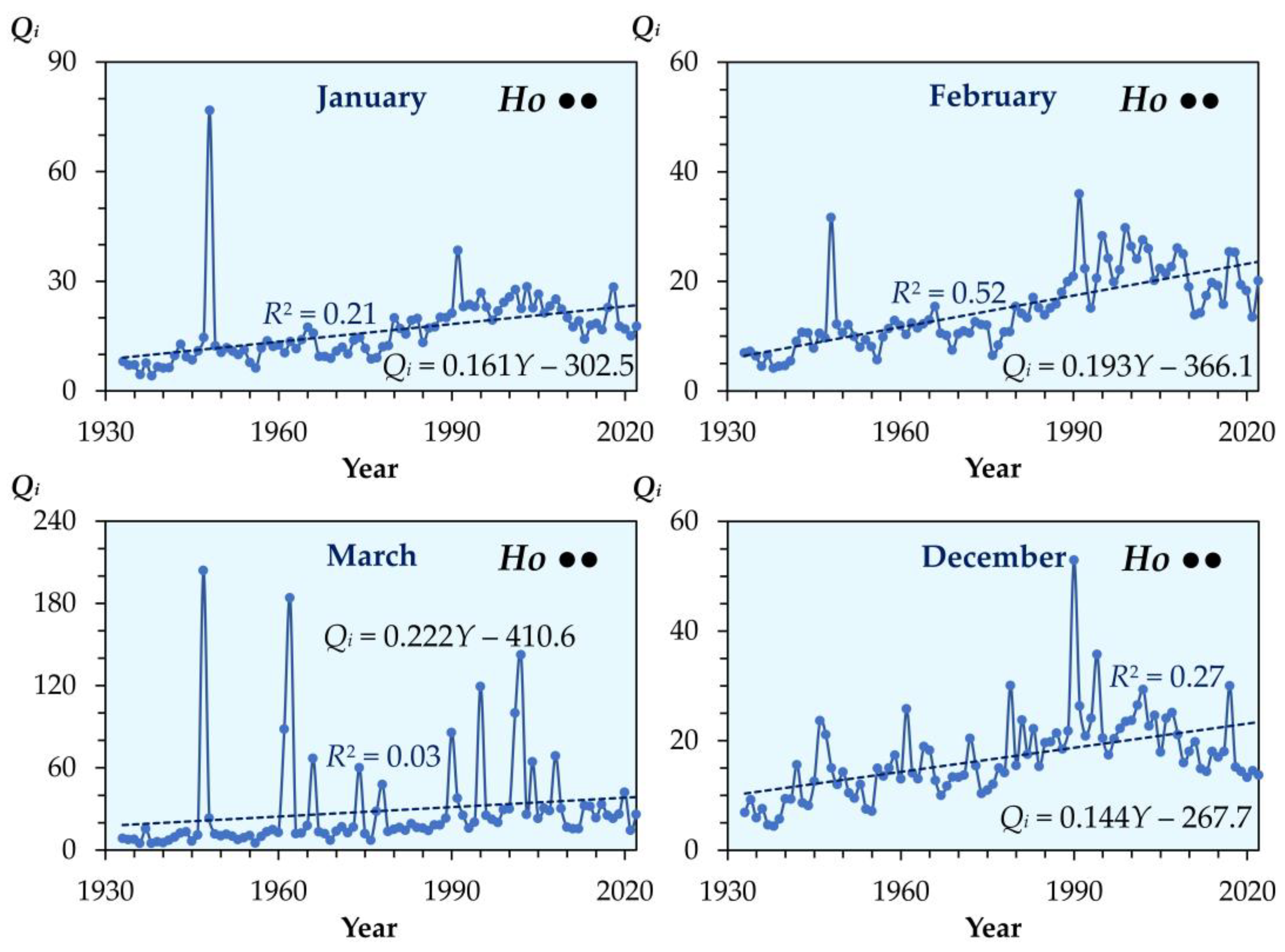
Figure A2.
Long-term trends in monthly mean discharges (Qi) of the Samara River at the Yelshanka gauging station during April and May, the months typically featuring the snowmelt flood (1933–2022). Ho and Ht indicate that the linearly detrended time series residuals are homoscedastic and heteroscedastic, respectively; a single bullet (•) denotes validation by only one statistical test, whereas a double bullet (••) denotes confirmation by both tests (see Table 1). For the remaining symbols, Figure A1.
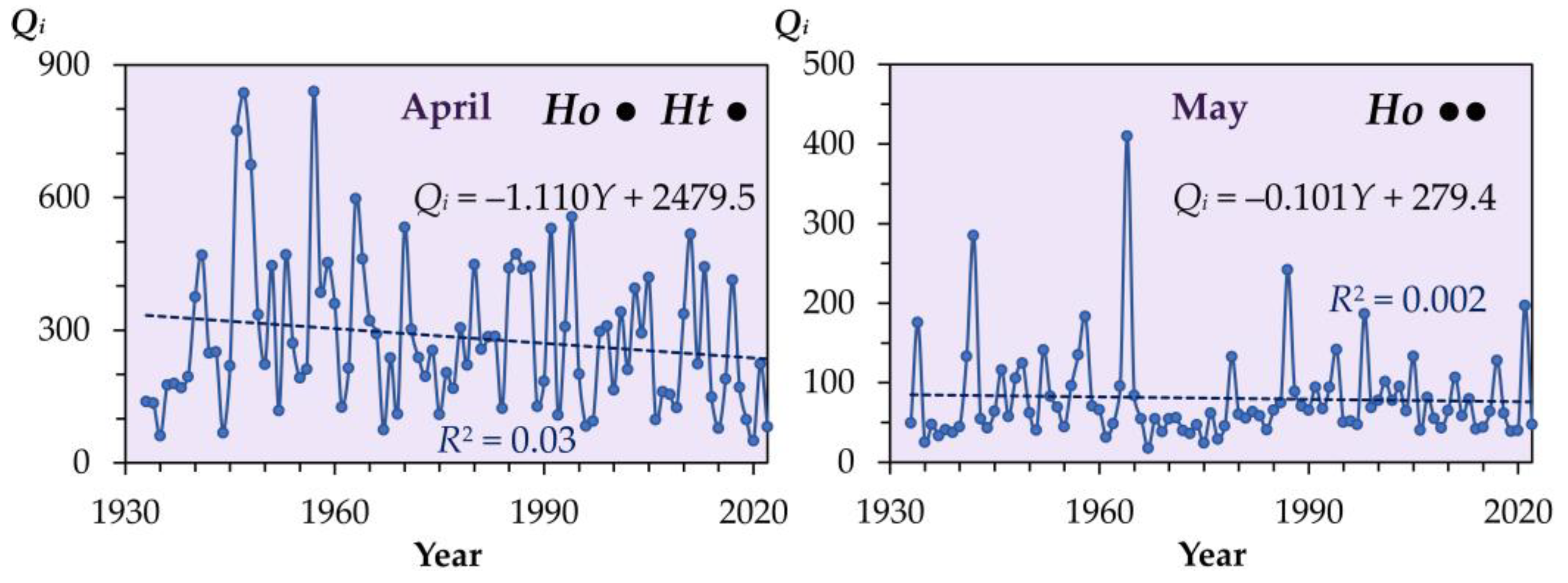
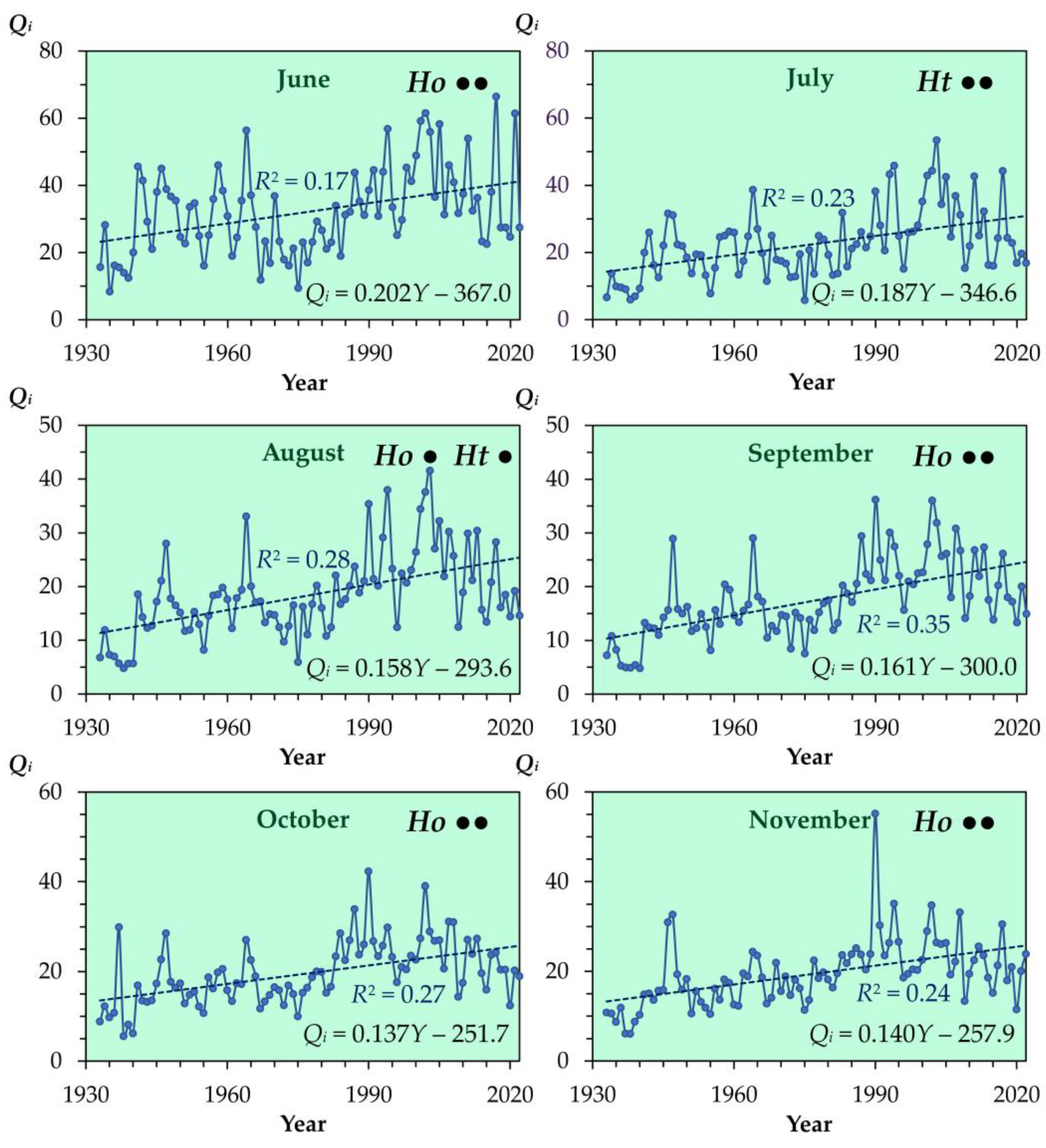
Figure A4.
Spearman’s rank correlation matrices between monthly mean discharge metrics for the Samara River at the Yelshanka gauging station across the analyzed climatological reference periods. The r value represents Spearman’s rank correlation coefficient. Roman numerals I–XII denote the calendar months (January–December); and Q represents the annual mean discharge.
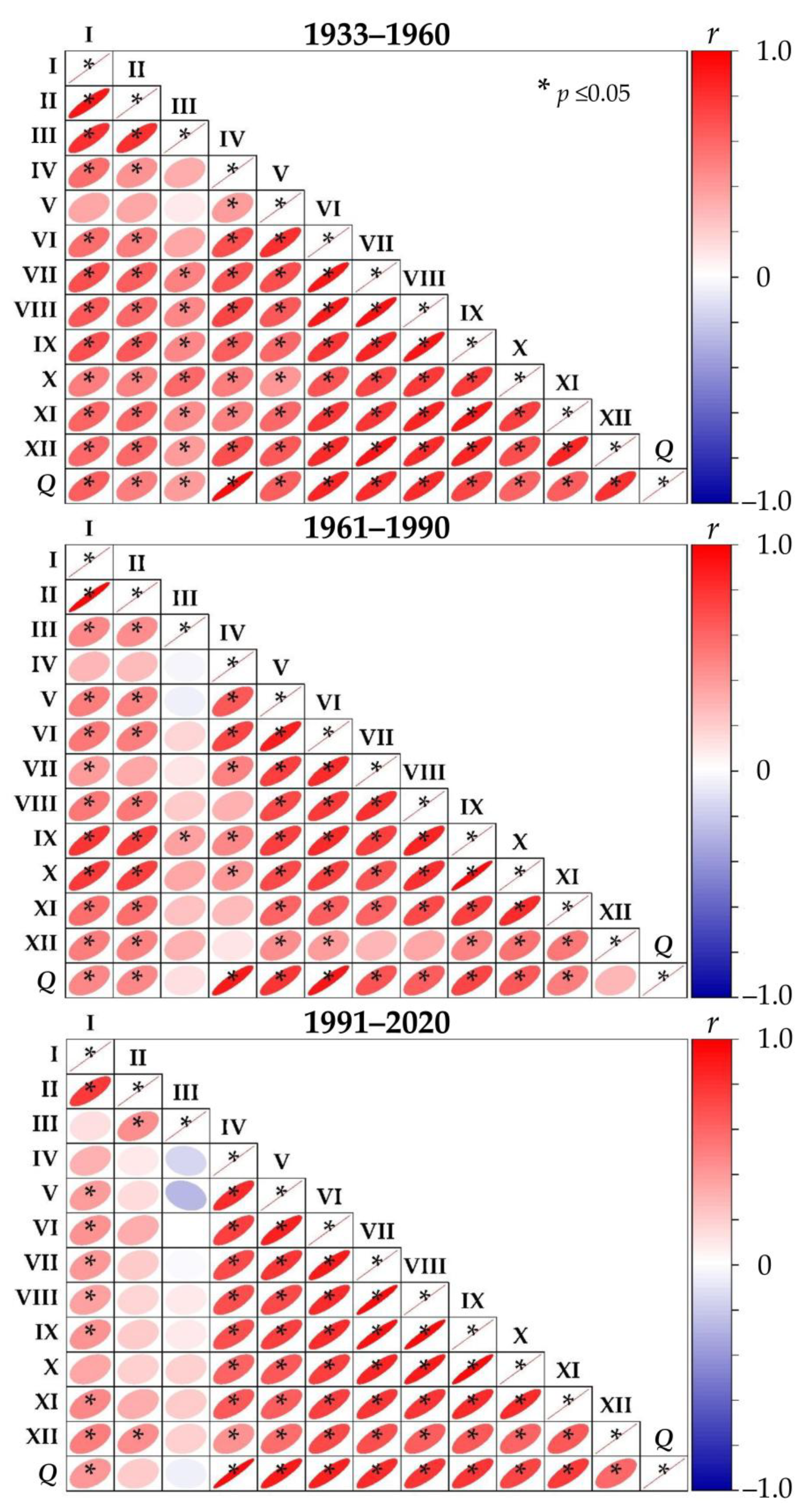
Figure A5.
Seasonal trend in monthly mean discharges (Qi, m3 s−1) of the Samara River at the Yelshanka gauging station during the 1933–2022 period.
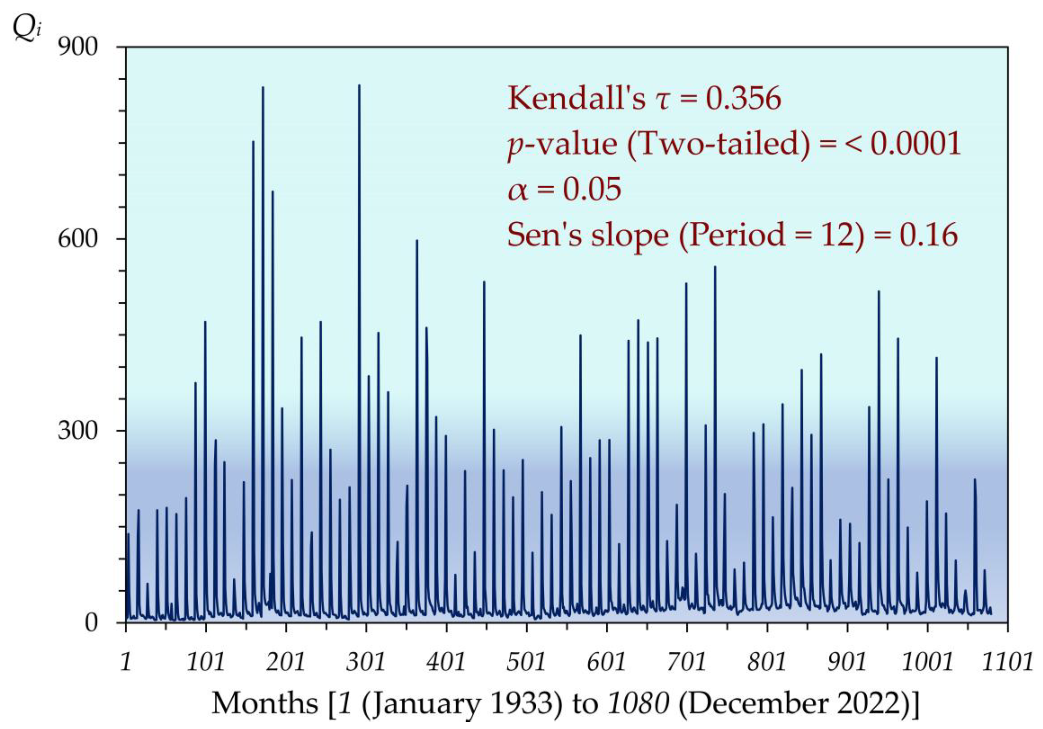
Figure A6.
Shifts in the proportional distribution (%) of runoff across calendar seasons and reference climatological periods in the Samara River at the Yelshanka gauging station. ∑—total annual runoff. The symbol Δ represents the relative change in the runoff proportion between the 1991–2020 and 1933–1960 periods; values in brackets indicate the number of years within each period. Statistical significance of differences between periods is based on the Mann–Whitney U and Kruskal–Wallis tests: n.s.—nonsignificant; * p < 0.05; ** p < 0.01; *** p < 0.001; **** p < 0.0001.
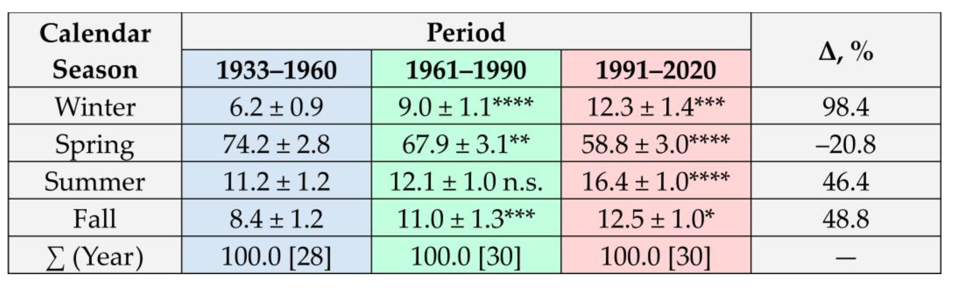
Figure A7.
Spectral density (SD, (m3 s−1)2/Hz) and corresponding periodicities (P) in monthly mean discharge values of the Samara River at the Yelshanka gauging station over the entire observation period (1933–2022). P1, P2, …, P6 denote the top six dominant periodicities in descending order of their variance contribution.
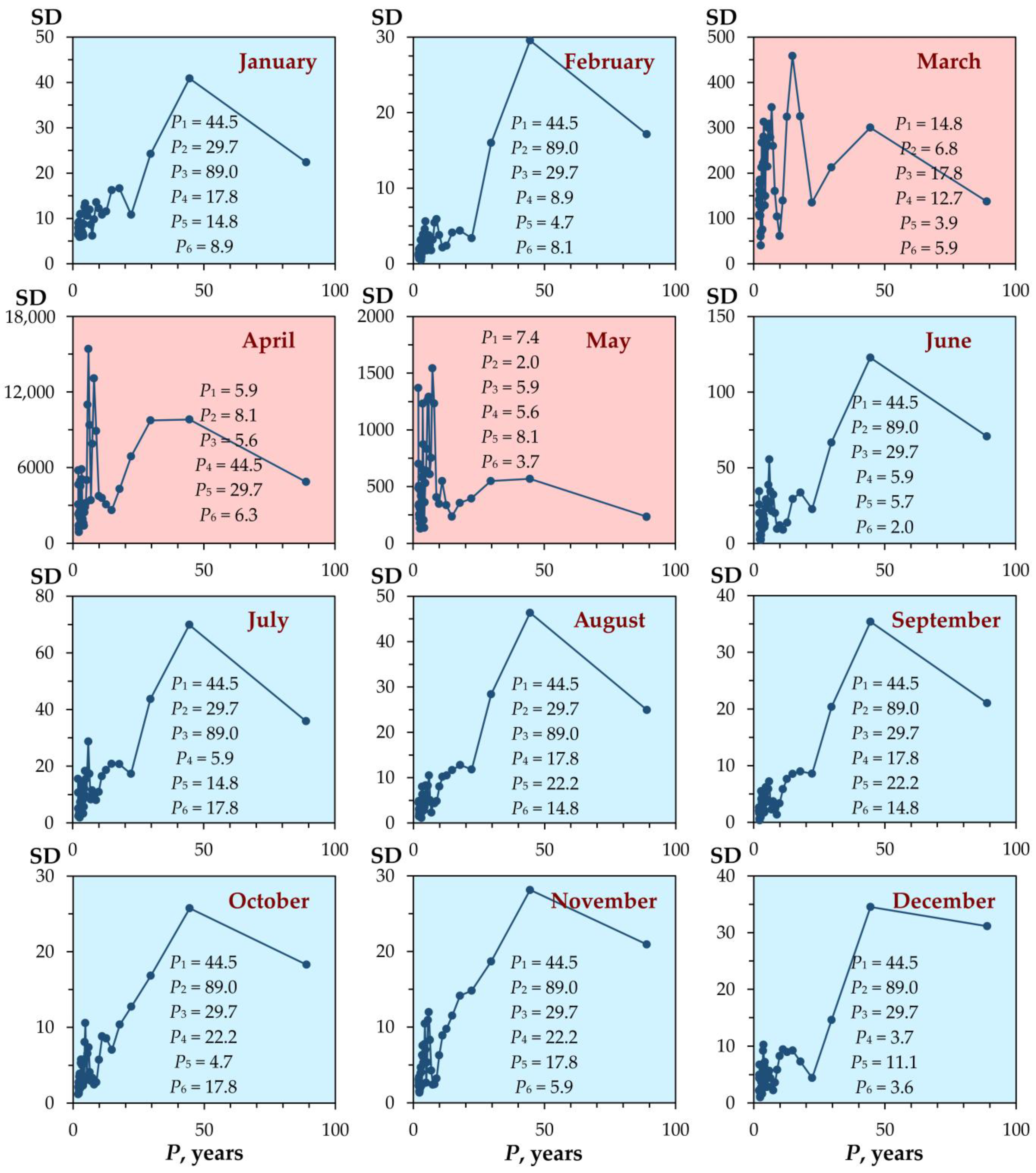
Figure A8.
Wavelet analysis results for the linearly detrended residuals of annual mean (εQ) and maximum monthly mean (εQmax) discharges of the Samara River at the Yelshanka gauging station over the entire observation period (1933–2022). The P value represents periodicity.
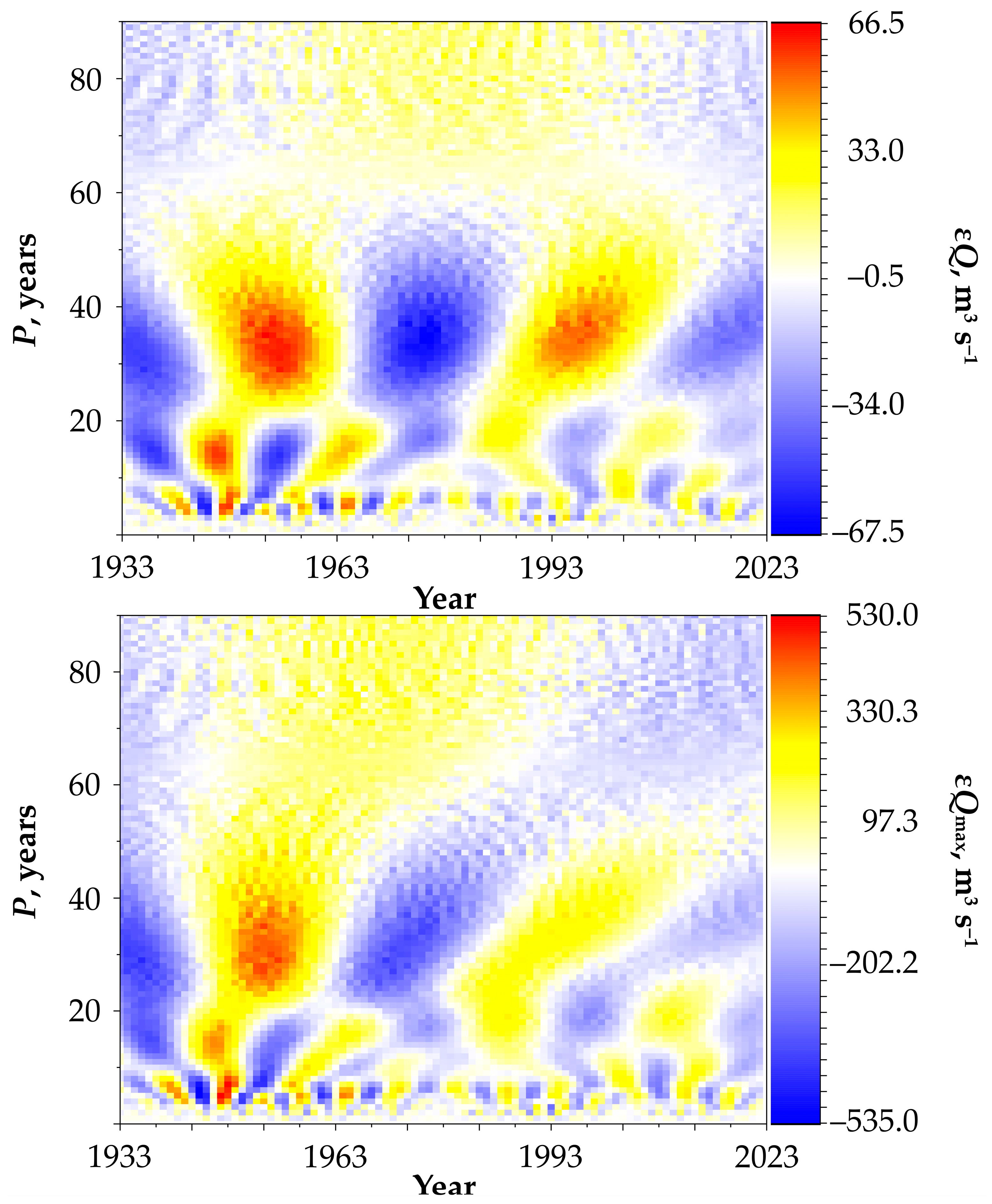
Figure A9.
Wavelet analysis results for the linearly detrended residuals of cold-season (εQmin-CS) and warm-season (εQmin-WS) minimum monthly mean discharges of the Samara River at the Yelshanka gauging station over the entire observation period (1933–2022). The P value represents periodicity.
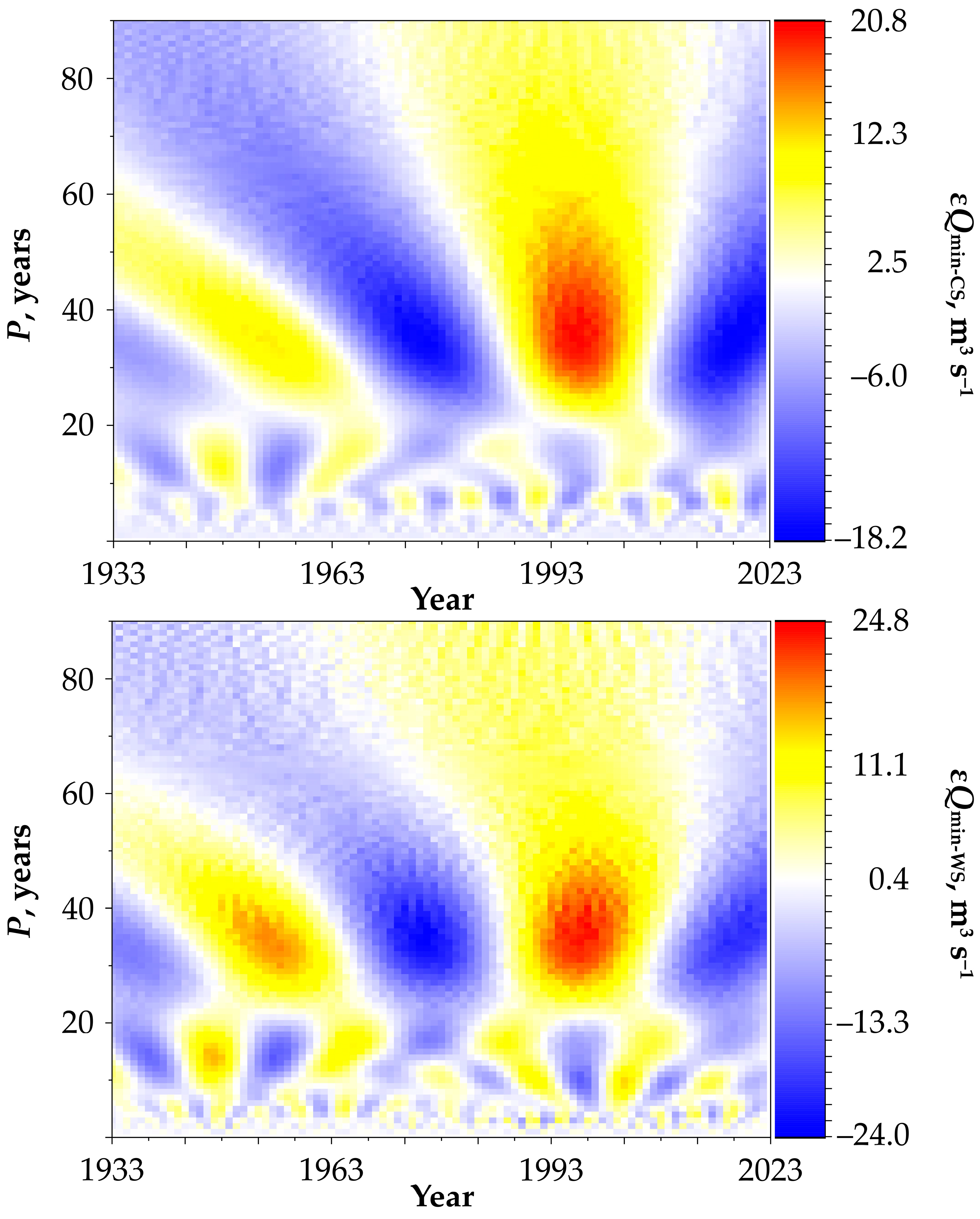
Figure A10.
Periodicities (P) in core hydrological variables (Q, Qmax, Qmin-CS, and Qmin-WS) of the Samara River at the Yelshanka gauging station over the reference climatological periods. P1, P2, and P3 denote the top three dominant periodicities in descending order of their variance contribution, where ∑ is their cumulative contribution to the total periodic runoff variability, and the brackets indicate the contribution share of periodicity P1.
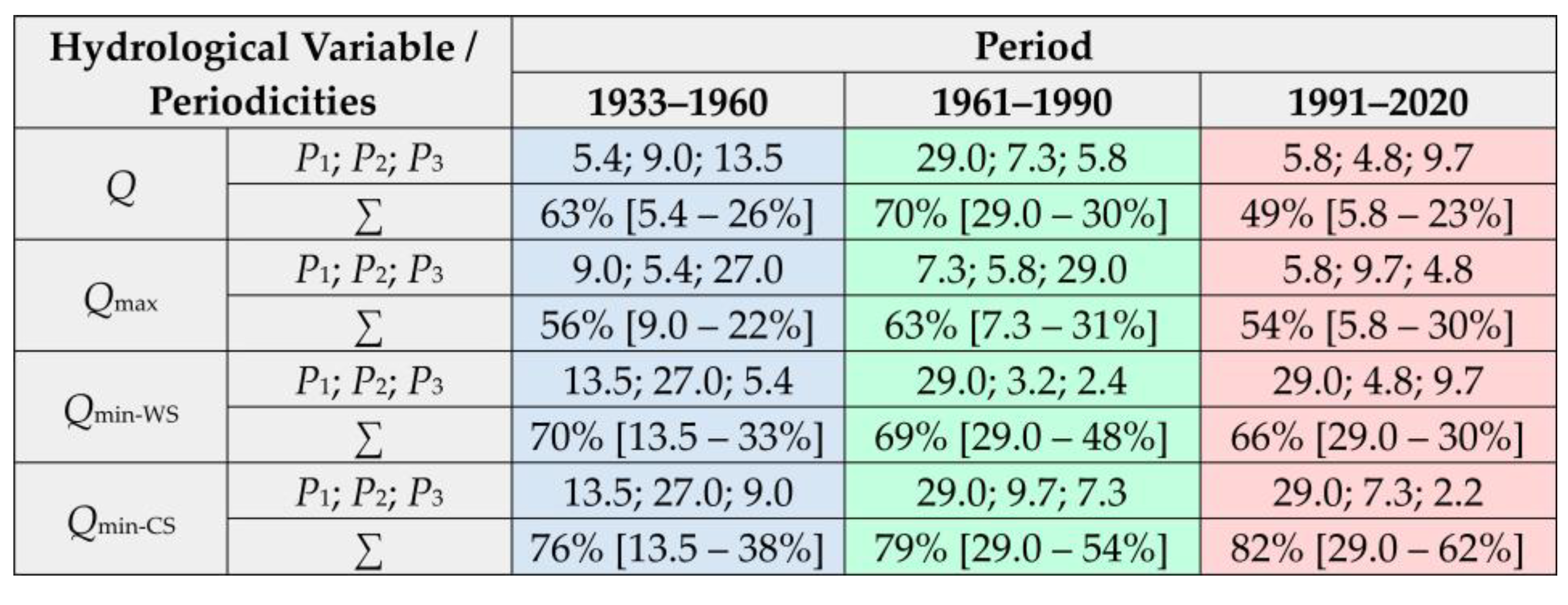
Figure A11.
Residual mass (Si) curves constructed from monthly mean discharge values for calendar seasons during the 1933–2022 period.
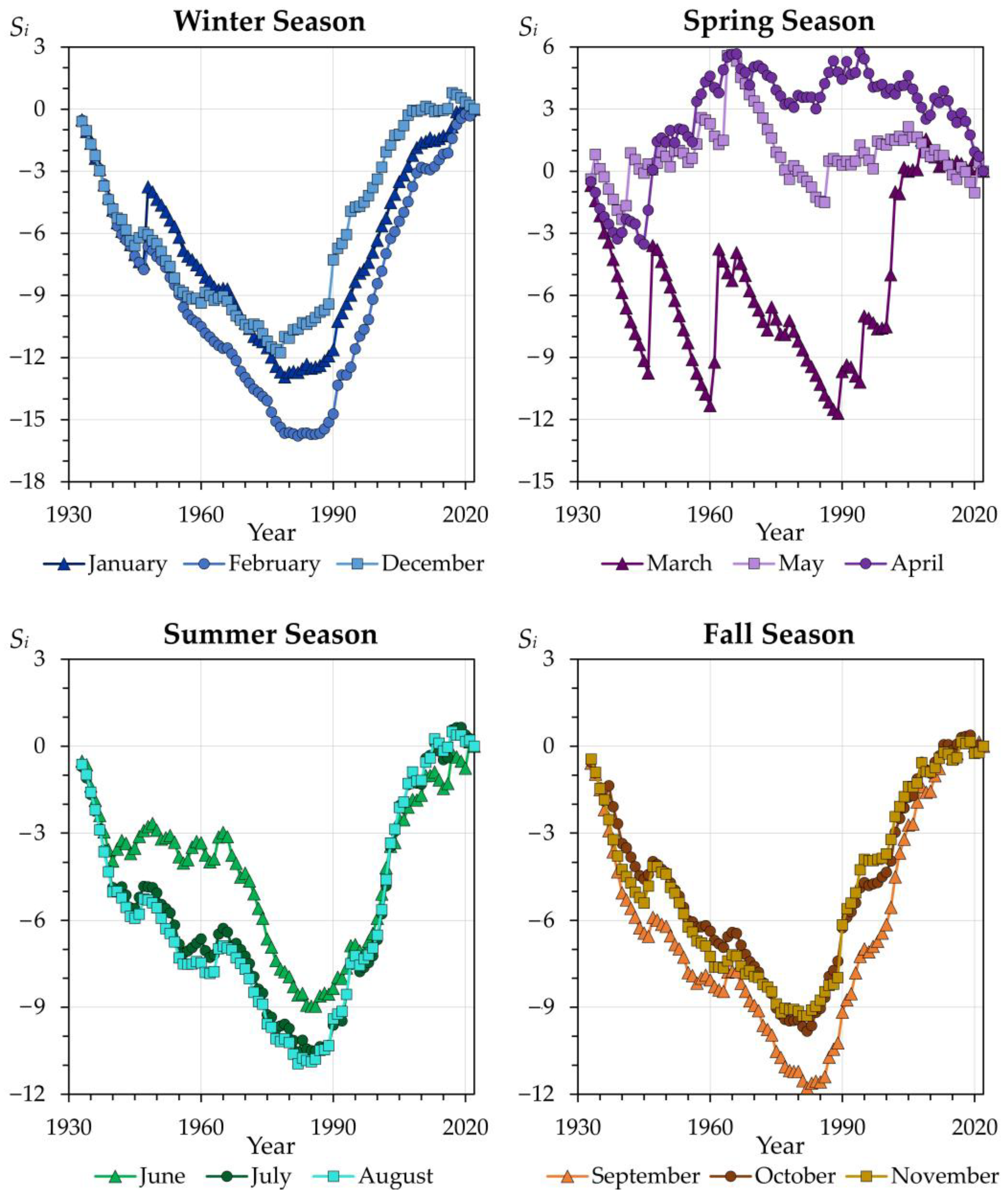
References
- Kiselev, A.A. (Ed.) Third Assessment Report on Climate Change and Its Consequences in the Russian Federation; Science-Intensive Technologies Publishing: Saint Petersburg, Russia, 2022. Available online: https://www.meteorf.gov.ru/upload/pdf_download/compressed.pdf (accessed on 15 June 2026). (In Russian)
- The Sixth Assessment Report (AR6) of the Intergovernmental Panel on Climate Change (IPCC). 2021. Available online: https://www.ipcc.ch/assessment-report/ar6/ (accessed on 20 June 2026).
- Paltán, H.A.; Folch, A.; Hope, R. Anthropogenic river flows. Environ. Res. Water 2026, 2, 033002. [Google Scholar]
- Popova, V.V.; Polyakova, I.A. Change of stable snow cover destruction dates in Northern Eurasia, 1936–2008: Impact of global warming and the role of large-scale atmospheric circulation. Ice Snow 2013, 53, 29–39. (In Russian) [Google Scholar]
- Park, H.; Sherstiukov, A.B.; Fedorov, A.N.; Polyakov, I.V.; Walsh, J.E. An observation-based assessment of the influences of air temperature and snow depth on soil temperature in Russia. Environ. Res. Lett. 2014, 9, 64026. [Google Scholar] [CrossRef] [Scilit]
- Ashabokov, B.A.; Tashilova, A.A.; Kesheva, L.A.; Taubekova, Z.A. Trends in precipitation parameters in the climate zones of southern Russia (1961–2011). Russ. Meteorol. Hydrol. 2017, 42, 150–158. [Google Scholar] [CrossRef] [Scilit]
- Perevedentsev, Y.; Gusarov, A.; Mirsaeva, N.; Sherstyukov, B.; Shantalinsky, K.; Guryanov, V.; Aukhadeev, T. Contemporary Climate Change and Its Hydrological Consequence in the Volga Federal District, European Russia. Climate 2022, 10, 198. [Google Scholar] [CrossRef] [Scilit]
- Hostert, P.; Kuemmerle, T.; Prishchepov, A.V.; Sieber, A.; Lambin, E.F.; Radeloff, V.C. Rapid land use change after socio-economic disturbances: The collapse of the Soviet Union versus Chernobyl. Environ. Res. Lett. 2011, 6, 045201. [Google Scholar] [CrossRef] [Scilit]
- Mukhin, G.D. Ecological-economic assessment of land use structure within the European territory of Russia during two recent decades. Vestn. Mosk. Univ. Ser. 5 Geogr. 2012, 5, 19–28. (In Russian) [Google Scholar]
- Nefedova, T.G. Major trends for changes in the socioeconomic space of rural Russia. Reg. Res. Russ. 2012, 2, 41–54. [Google Scholar] [CrossRef] [Scilit]
- Prishchepov, A.V.; Müller, D.; Dubinin, M.; Baumann, M.; Radeloff, V.C. Determinants of agricultural land abandonment in post-Soviet European Russia. Land Use Policy 2013, 30, 873–884. [Google Scholar] [CrossRef] [Scilit]
- Lyuri, D.I.; Nekrich, A.S.; Karelin, D.V. Cropland dynamics in Russia in 1990–2015 and soil emission of carbon dioxide. Vest. Mosk. Univ. Ser. 5 Geogr. 2018, 3, 70–76. (In Russian) [Google Scholar]
- Nekrich, A.S.; Lyuri, D.I. Changes of the dynamic of agrarian lands of Russia in 1990–2014. Izv. Ross. Akad. Nauk. Seriya Geogr. 2019, 3, 64–77. (In Russian) [Google Scholar] [CrossRef] [Scilit]
- Poesen, J. Soil erosion in the Anthropocene: Research needs. Earth Surf. Process. Landf. 2018, 43, 64–84. [Google Scholar] [CrossRef] [Scilit]
- Cendrero, A.; Remondo, J.; Beylich, A.A.; Cienciala, P.; Forte, L.M.; Golosov, V.N.; Gusarov, A.V.; Kijowska-Strugała, M.; Laute, K.; Li, D.; et al. Denudation and geomorphic change in the Anthropocene; a global overview. Earth-Sci. Rev. 2022, 233, 104186. [Google Scholar] [CrossRef] [Scilit]
- Syvitski, J.; Restrepo-Ángel, J.; Saito, Y.; Overeem, I.; Vörösmarty, C.J.; Wang, H.; Olago, D. Earth’s sediment cycle during the Anthropocene. Nat. Rev. Earth Environ. 2022, 3, 179–196. [Google Scholar] [CrossRef] [Scilit]
- O’Hara, K.D. Climate Change in the Anthropocene; Elsevier: Amsterdam, The Netherlands; Oxford, UK; Cambridge, MA, USA, 2022. [Google Scholar]
- Lewis, S.; Maslin, M.A. Defining the Anthropocene. Nature 2015, 519, 171–180. [Google Scholar] [CrossRef] [Scilit] [PubMed]
- Zalasiewicz, J.; Waters, C.N.; Williams, M.; Barnosky, A.D.; Cearreta, A.; Crutzen, P.; Ellis, E.; Ellis, M.A.; Fairchild, I.J.; Grinevald, J.; et al. When did the Anthropocene begin? A mid-twentieth century boundary level is stratigraphically optimal. Quat. Int. 2015, 383, 204–207. [Google Scholar] [CrossRef] [Scilit]
- Steffen, W.; Leinfelder, R.; Zalasiewicz, J.; Waters, C.N.; Williams, M.; Summerhayes, C.; Barnosky, A.D.; Cearreta, A.; Crutzen, P.; Edgeworth, M.; et al. Stratigraphic and Earth System approaches to defining the Anthropocene. Earth’s Future 2016, 4, 324–345. [Google Scholar] [CrossRef] [Scilit]
- Cao, Z.; Wang, S.; Luo, P.; Xie, D.; Zhu, W. Watershed Ecohydrological Processes in a Changing Environment: Opportunities and Challenges. Water 2022, 14, 1502. [Google Scholar] [CrossRef] [Scilit]
- LeRoy Poff, N. Rivers of the Anthropocene? Front. Ecol. Environ. 2014, 12, 427. [Google Scholar] [CrossRef] [Scilit]
- Collier, M.J.; Devitt, C. Novel ecosystems: Challenges and opportunities for the Anthropocene. Anthr. Rev. 2016, 3, 231–242. [Google Scholar] [CrossRef] [Scilit]
- Wohl, E. Rivers in the Anthropocene: The U.S. perspective. Geomorphology 2020, 366, 106600. [Google Scholar] [CrossRef] [Scilit]
- Sun, G.; Hallema, D.; Asbjornsen, H. Ecohydrological processes and ecosystem services in the Anthropocene: A review. Ecol. Process. 2017, 6, 35. [Google Scholar] [CrossRef] [Scilit]
- DeBoer, J.A.; Thoms, M.C.; Delong, D.M. The Anthropocene: Rivers and resilience. In Resilience and Riverine Landscapes, 1st ed.; Thoms, M., Fuller, I., Eds.; Elsevier: Amsterdam, The Netherlands, 2024; pp. 209–228. [Google Scholar] [CrossRef] [Scilit]
- Szczepocka, E.; Żelazna-Wieczorek, J.; Zakrzewski, P.K. Impact of urbanization-driven changes of the riverbeds on its ecological status evidenced by diatom communities—The negative side of the Anthropocene. Ecol. Indic. 2024, 159, 111706. [Google Scholar] [CrossRef] [Scilit]
- Gelfan, A.N.; Frolova, N.L.; Magritsky, D.V.; Kireeva, M.B.; Grigoriev, V.Y.; Motovilov, Y.G.; Gusev, E.M. Climate change impact on the annual and maximum runoff of Russian rivers: Diagnosis and projections. Izv. Atmos. Ocean. Phys. 2023, 59, 153–169. [Google Scholar] [CrossRef] [Scilit]
- Frolova, N.L.; Kireeva, M.B.; Agafonova, S.A.; Yevstigneev, V.M.; Yefremova, N.A.; Povalishnikova, Y.S. Intra-annual distribution of the plain river discharges within the European Russia and its change. Water Sect. Russ. Probl. Technol. Manag. 2015, 4, 4–20. (In Russian) [Google Scholar]
- Frolova, N.L.; Agafonova, S.; Kireeva, M.B.; Povalishnikova, E.S.; Pakhomova, O.M. Recent changes of annual flow distribution of the Volga basin rivers. Geogr. Environ. Sustain. 2017, 10, 28–39. [Google Scholar] [CrossRef] [Scilit]
- Dzhamalov, R.G.; Rets, E.P.; Bugrov, A.A.; Frolova, N.L. Formation of current groundwater resources in European Russia. Water Resour. 2015, 42, 563–571. [Google Scholar] [CrossRef] [Scilit]
- Dolgov, S.V.; Koronkevich, N.I.; Barabanova, E.A. Modern alterations of the surface runoff and infiltration of melt water in agricultural fields in the forest-steppe and steppe zones of the Russian Plain and their consequence. Water Sect. Russ. Probl. Technol. Manag. 2018, 4, 78–91. (In Russian) [Google Scholar] [CrossRef] [Scilit]
- Koronkevich, N.I.; Georgiadi, A.G.; Dolgov, S.V.; Barabanova, E.A.; Kashutina, E.A.; Milyukova, I.P. Change in snow flood flow in the southern macro-slope of the Russian Plain in the period 1930–2014. Ice Snow 2018, 58, 498–506. (In Russian) [Google Scholar] [CrossRef] [Scilit]
- Gusarov, A.V. The impact of contemporary changes in climate and land use/cover on tendencies in water flow, suspended sediment yield and erosion intensity in the northeastern part of the Don River basin, SW European Russia. Environ. Res. 2019, 175, 468–488. [Google Scholar] [CrossRef] [Scilit] [PubMed]
- Sivokhip, Z.T.; Pavleichik, V.M.; Padalko, Y.A. Change in the minimum runoff of the Ural River basin. Izv. Ross. Akad. Nauk. Seriya Geogr. 2021, 85, 900–913. (In Russian) [Google Scholar]
- Filippova, I.A. Minimum Flow of Rivers in the European Territory of Russia and Its Assessment in the Context of Climate Change. Ph.D. Thesis, Institute of Water Problems of the Russian Academy of Sciences, Moscow, Russia, 2014. Available online: https://www.iwp.ru/upload/iblock/0ce/0ceb3c09474b805c2ae7597c5a3be865.pdf (accessed on 17 May 2026). (In Russian)
- Dzhamalov, R.G.; Frolova, N.L.; Kireeva, M.B. Current changes in river water regime in the Don River basin. Water Resour. 2013, 40, 573–584. [Google Scholar] [CrossRef] [Scilit]
- Bolgov, M.V.; Korobkina, E.A.; Trubetskova, M.D.; Filimonova, M.K.; Filippova, I.A. Present-day variations of the minimum runoff of the Volga Basin rivers. Russ. Meteorol. Hydrol. 2014, 39, 187–194. [Google Scholar] [CrossRef] [Scilit]
- Bolgov, M.V.; Trubetskova, M.D.; Filimonova, M.K.; Filippova, I.A. Modern alterations of climate characteristics and probabilistic assessment of the minimal flow alterations in the Volga River basin. Water Sect. Russ. Probl. Technol. Manag. 2014, 3, 83–99. (In Russian) [Google Scholar] [CrossRef] [Scilit]
- Blöschl, G.; Hall, J.; Parajka, J.; Perdigão, R.A.P.; Merz, B.; Arheimer, B.; Aronica, G.T.; Bilibashi, A.; Bonacci, O.; Borga, M.; et al. Changing climate shifts timing of European floods. Science 2017, 357, 588–590. [Google Scholar] [CrossRef] [Scilit] [PubMed]
- Blöschl, G.; Hall, J.; Viglione, A.; Perdigão, R.A.P.; Parajka, J.; Merz, B.; Lun, D.; Arheimer, B.; Aronica, G.T.; Bilibashi, A.; et al. Changing climate both increases and decreases European river floods. Nature 2019, 573, 108–111. [Google Scholar] [CrossRef] [Scilit] [PubMed]
- Šarauskienė, D.; Kriaučiūnienė, J.; Jakimavičius, D.; Biliūnaitė, A. Flood Characterisation in Lithuanian Lowland Rivers Using a Peaks-over-Threshold Approach. Water 2026, 18, 1033. [Google Scholar] [CrossRef] [Scilit]
- Arheimer, B.; Lindström, G. Climate impact on floods: Changes in high flows in Sweden in the past and the future (1911–2100). Hydrol. Earth Syst. Sci. 2015, 19, 771–784. [Google Scholar] [CrossRef] [Scilit]
- Kaczmarek, Z. The impact of climate variability on flood risk in Poland. Risk Anal. 2003, 23, 559–566. [Google Scholar] [CrossRef] [Scilit] [PubMed]
- Chibilev, A.A. (Ed.) Geographical Atlas of the Orenburg Oblast. 024–027. Air Temperature and Mean Annual Precipitation; DIK Publishing: Moscow, Russia, 1999; Available online: https://geoportal.rgo.ru/record/7452/ (accessed on 27 August 2026). (In Russian)
- Levitin, I.E.; Borodko, A.V. (Eds.) National Atlas of Russia. Chapter 2 “Nature. Ecology”, Sec. 9: Soil Cover and Land Resources; Roskartografiya Publishing: Moscow, Russia, 2007; Available online: https://nationalatlas.ru/tom2/298-301.html/ (accessed on 25 July 2026). (In Russian)
- Levitin, I.E.; Borodko, A.V. (Eds.) National Atlas of Russia. Chapter 2 “Nature. Ecology”, Sec. 10: Vegetation; Roskartografiya Publishing: Moscow, Russia, 2007; Available online: https://nationalatlas.ru/tom2/328-330.html/ (accessed on 25 July 2026). (In Russian)
- Golosov, V.N.; Yermolaev, O.P. (Eds.) Spatiotemporal Patterns of Contemporary Processes Dynamics of Natural and Human-Induced Erosion on Agricultural Lands of the Russian Plain; Publishing House of the Academy of Sciences of the Republic of Tatarstan: Kazan, Russia, 2019. (In Russian) [Google Scholar]
- Barabanov, A.T. Specific features of spring slope runoff formation on arable lands of the Lower Volga River region. Vestn. Mosk. Univ. Seriya 5 Geogr. 2021, 6, 77–86. (In Russian) [Google Scholar]
- Barabanov, A.T.; Petelko, A.I. Factors of slope spring runoff on gray forest soils in the central forest-steppe. Lomonosov Geogr. J. 2023, 78, 18–27. (In Russian) [Google Scholar] [CrossRef] [Scilit]
- Gusarov, A.V. The response of water flow, suspended sediment yield and erosion intensity to contemporary long-term changes in climate and land use/cover in river basins of the Middle Volga Region, European Russia. Sci. Total Environ. 2020, 719, 134770. [Google Scholar] [CrossRef] [Scilit] [PubMed]
- Gusarov, A.V.; Beylich, A.A. Anthropocene Trends in Water Flow of Small and Medium-Sized Rivers in the East of the East European Plain: The Forest-Steppe and Steppe Zones. Hydrology 2025, 12, 242. [Google Scholar] [CrossRef] [Scilit]
- Chernokulsky, A.; Kozlov, F.; Zolina, O.; Bulygina, O.; Mokhov, I.I.; Semenov, V.A. Observed changes in convective and stratiform precipitation in Northern Eurasia over the last five decades. Environ. Res. Lett. 2019, 14, 045001. [Google Scholar] [CrossRef] [Scilit]
- Gusarov, A.V. Land-use/-cover changes and their effect on soil erosion and river suspended sediment load in different landscape zones of European Russia during 1970–2017. Water 2021, 13, 1631. [Google Scholar] [CrossRef] [Scilit]
- Gusarov, A.V.; Sharifullin, A.G.; Beylich, A.A. Contemporary Trends in River Flow, Suspended Sediment Load, and Soil/Gully Erosion in the South of the Boreal Forest Zone of European Russia: The Vyatka River Basin. Water 2021, 13, 2567. [Google Scholar] [CrossRef] [Scilit]
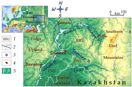
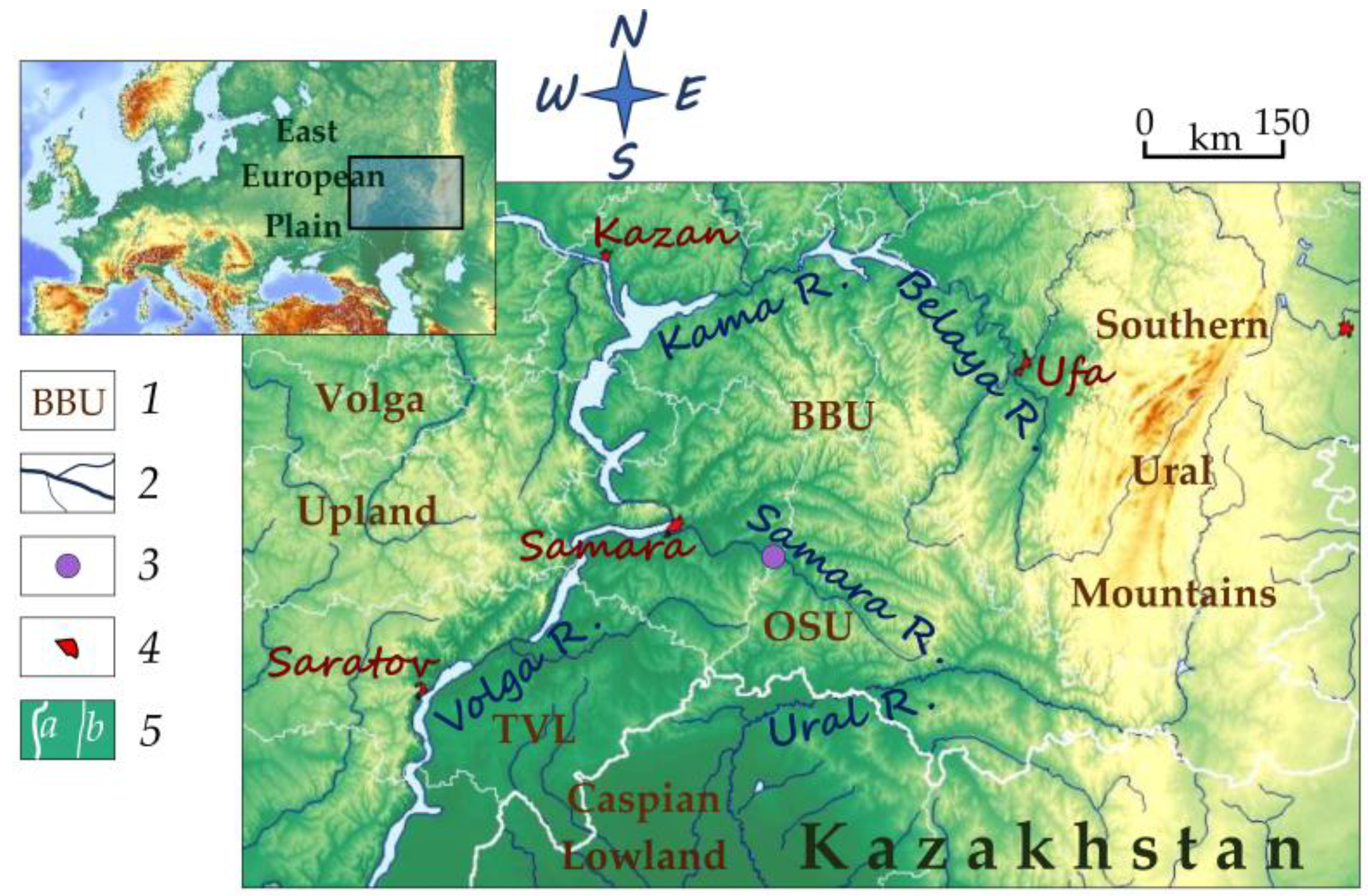
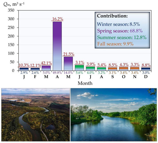
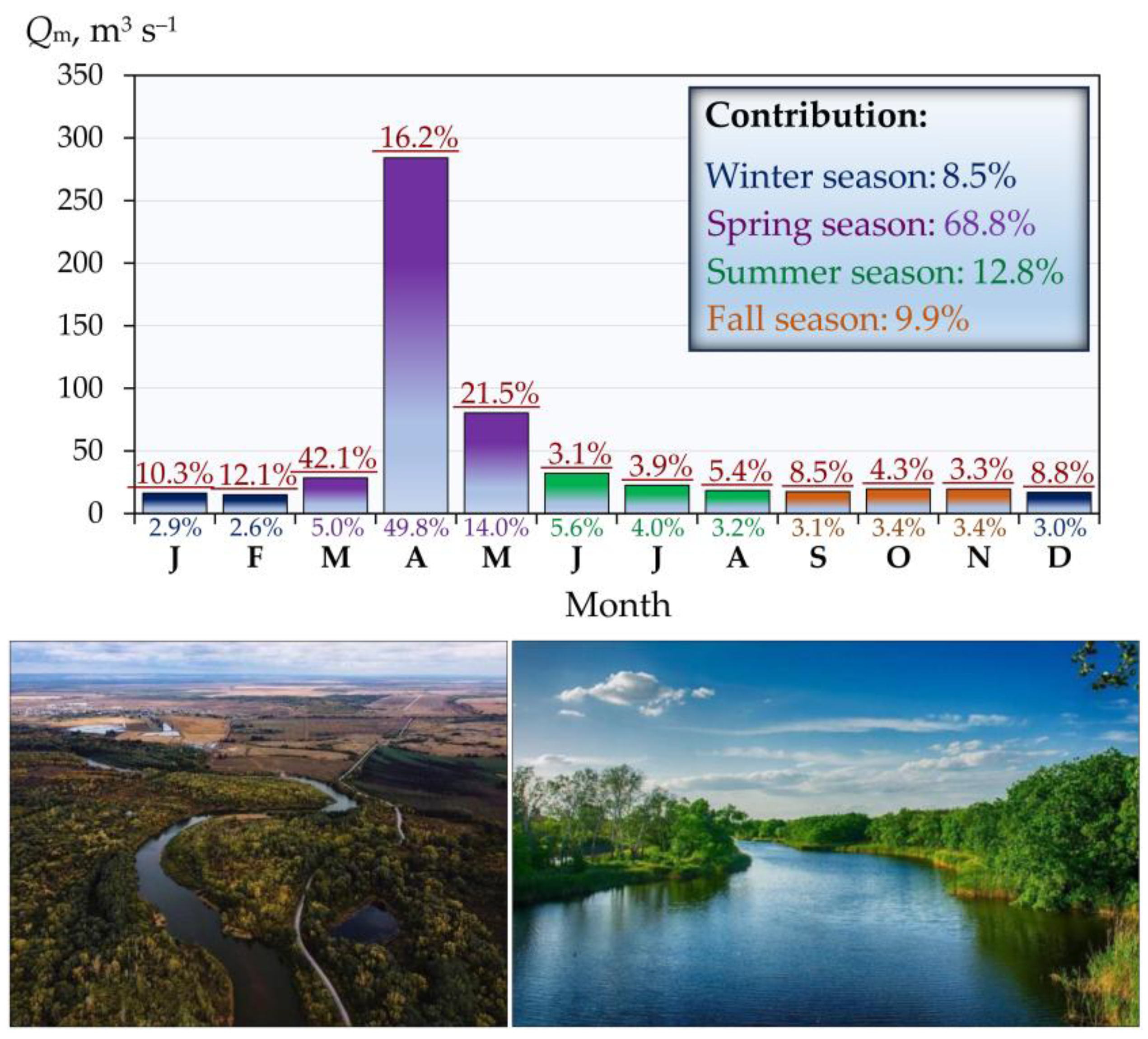
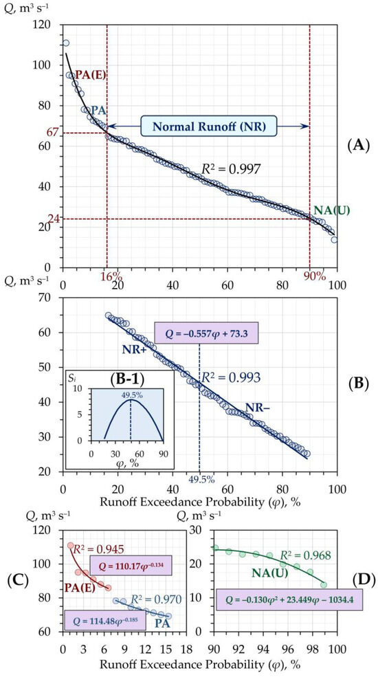
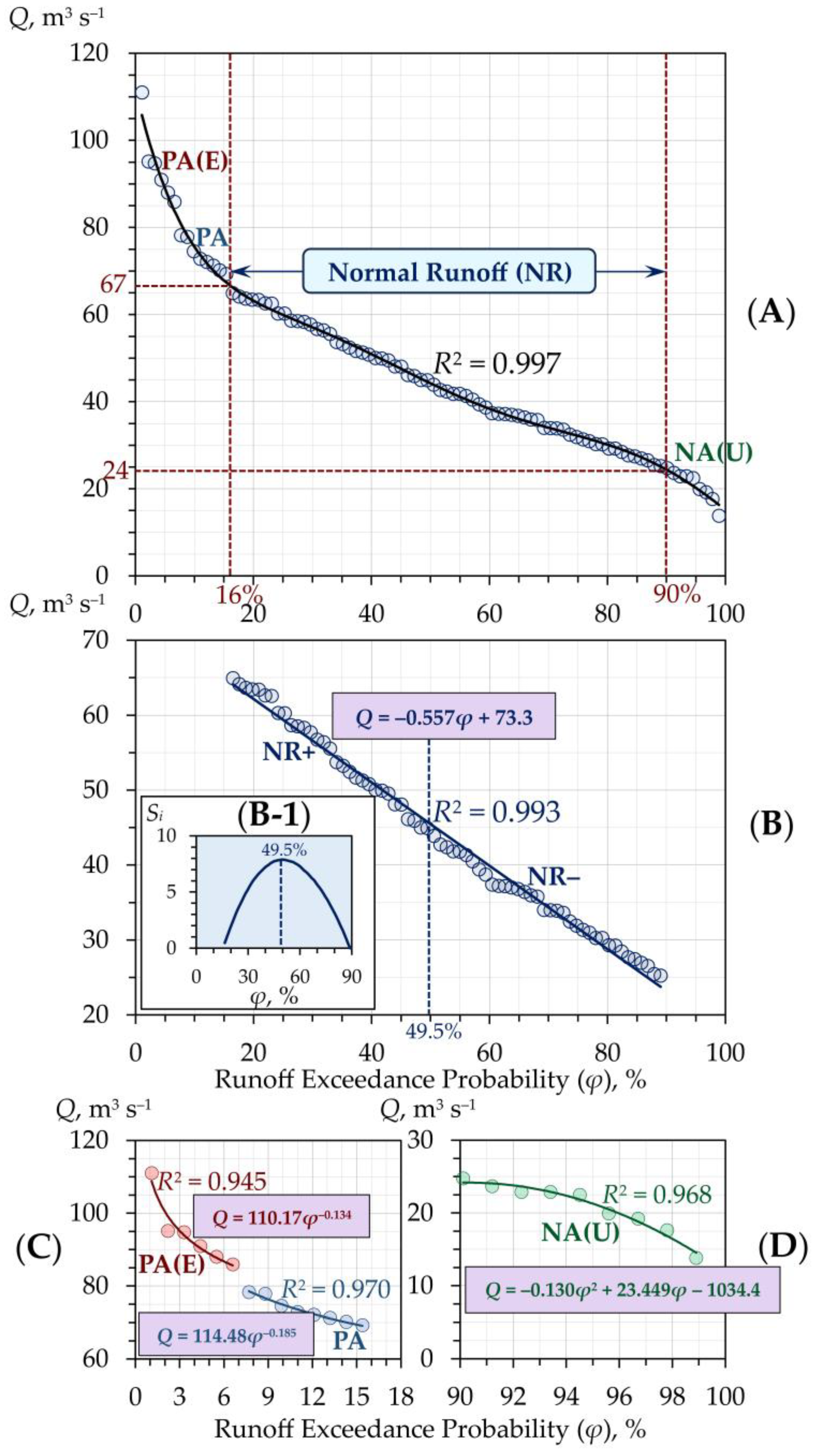
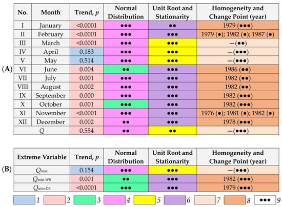
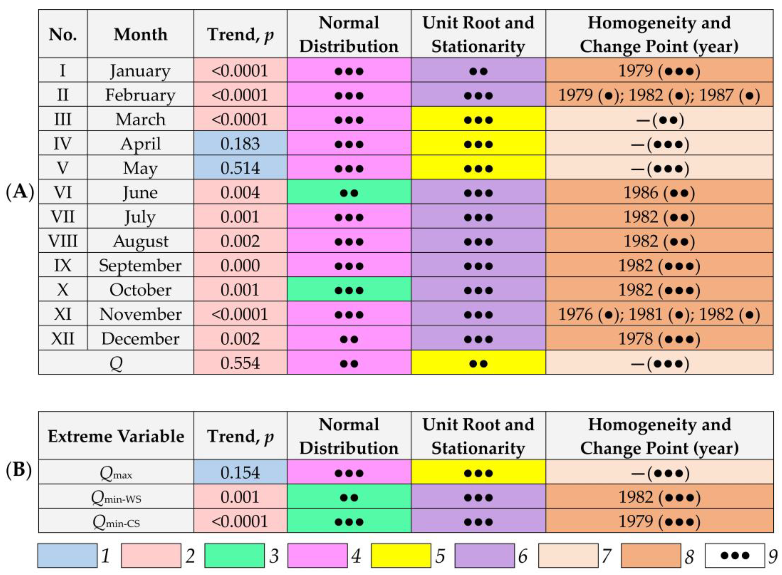
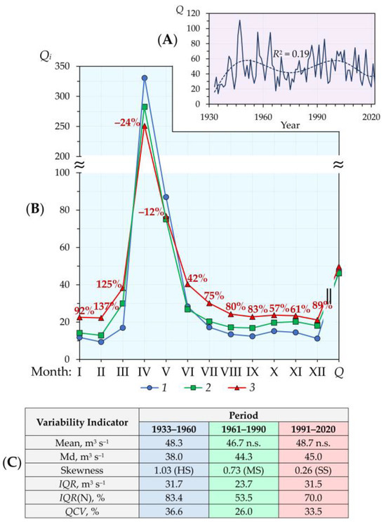
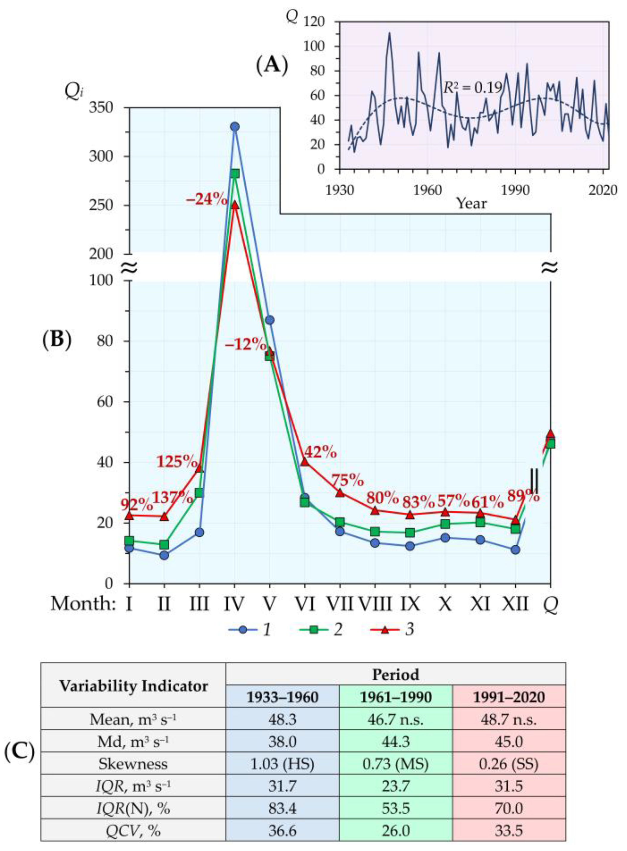
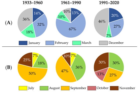
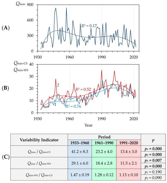
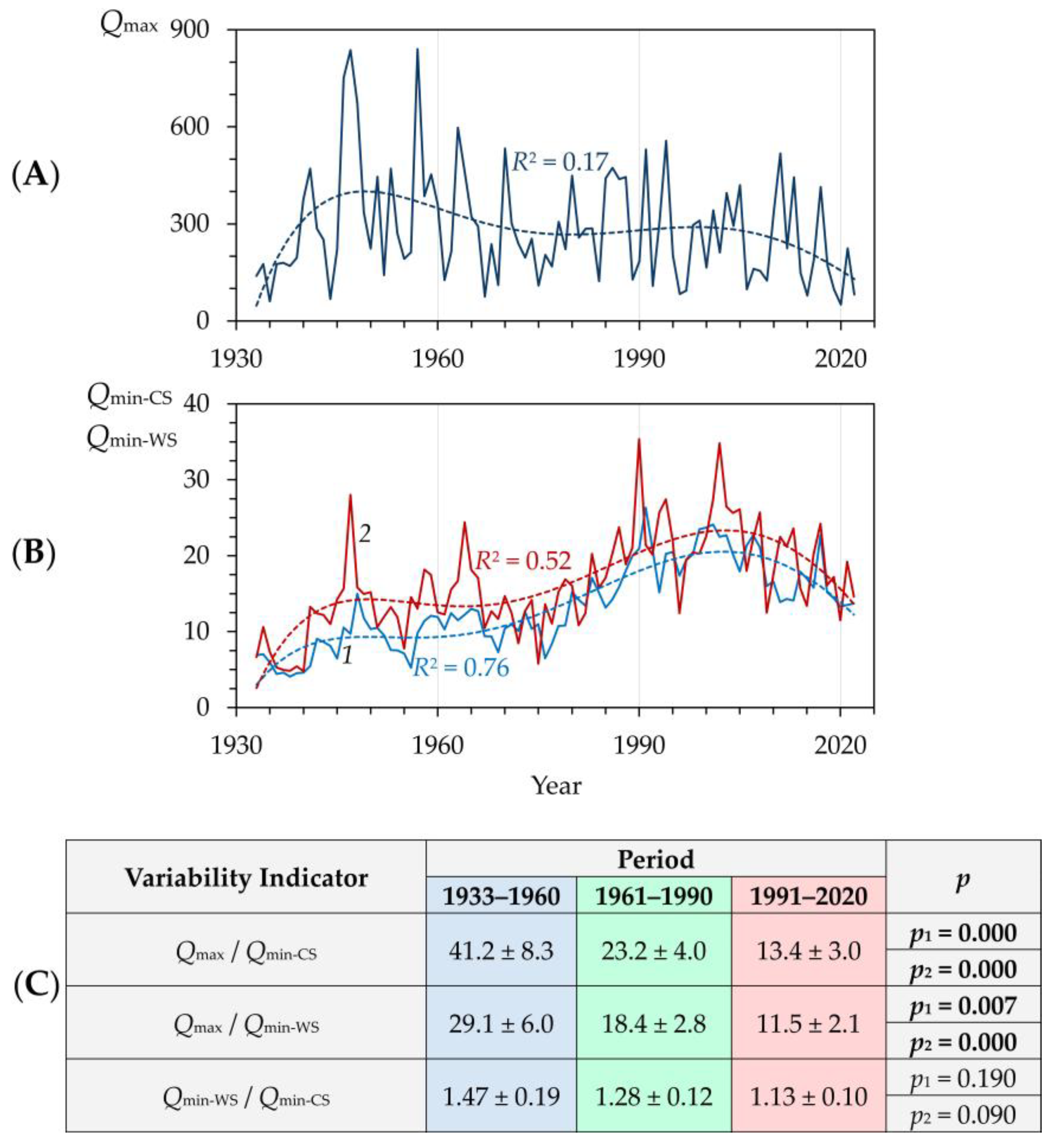
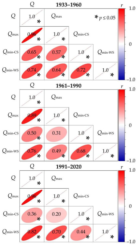
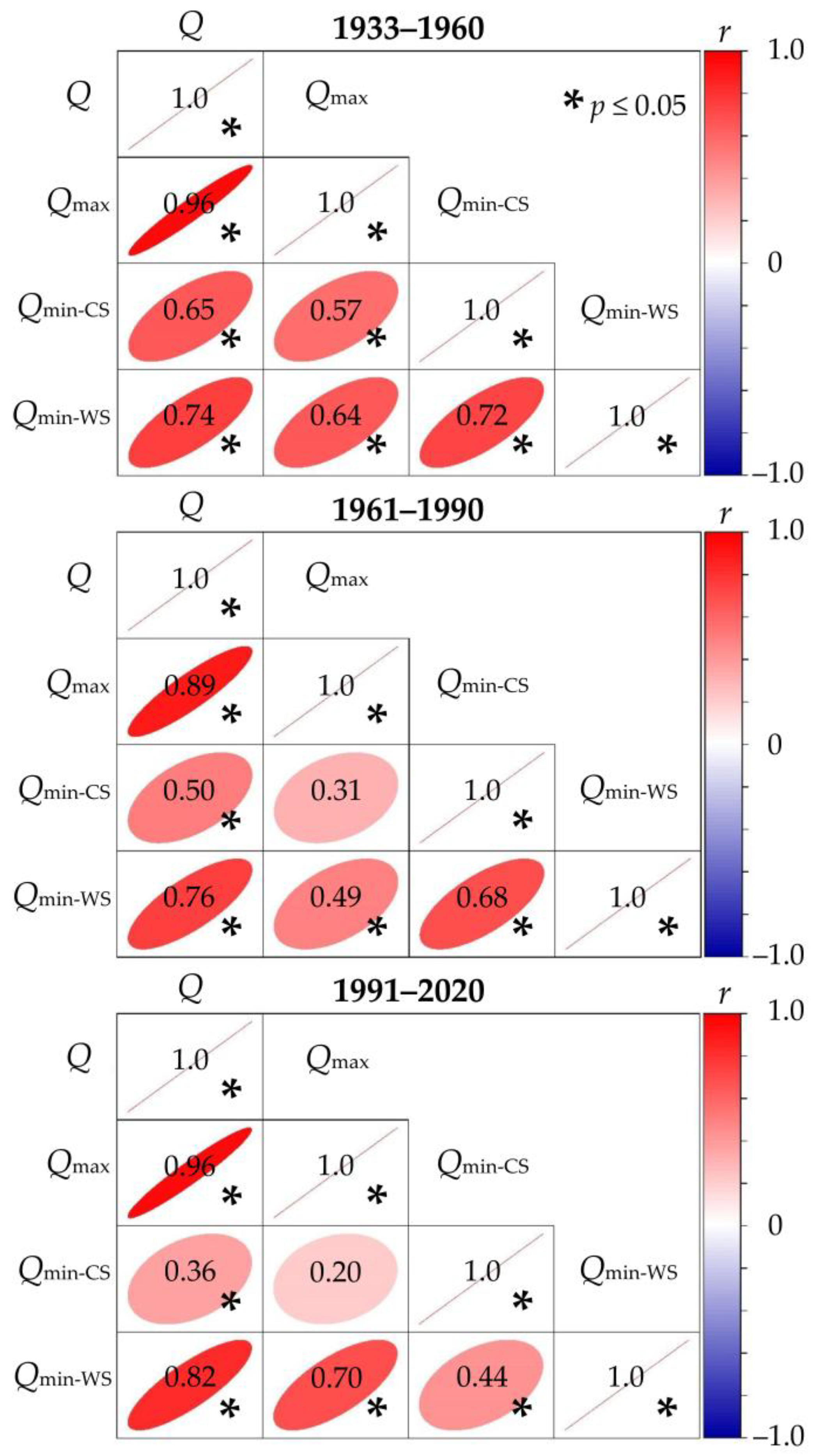
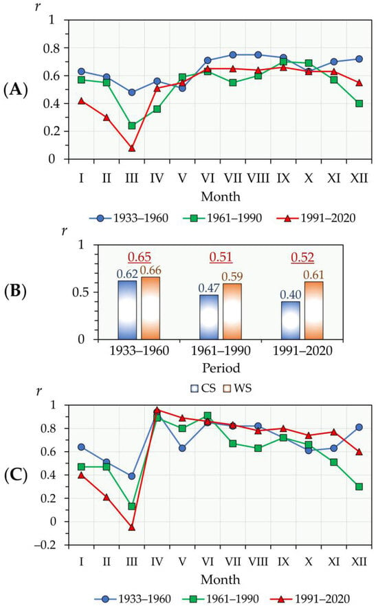
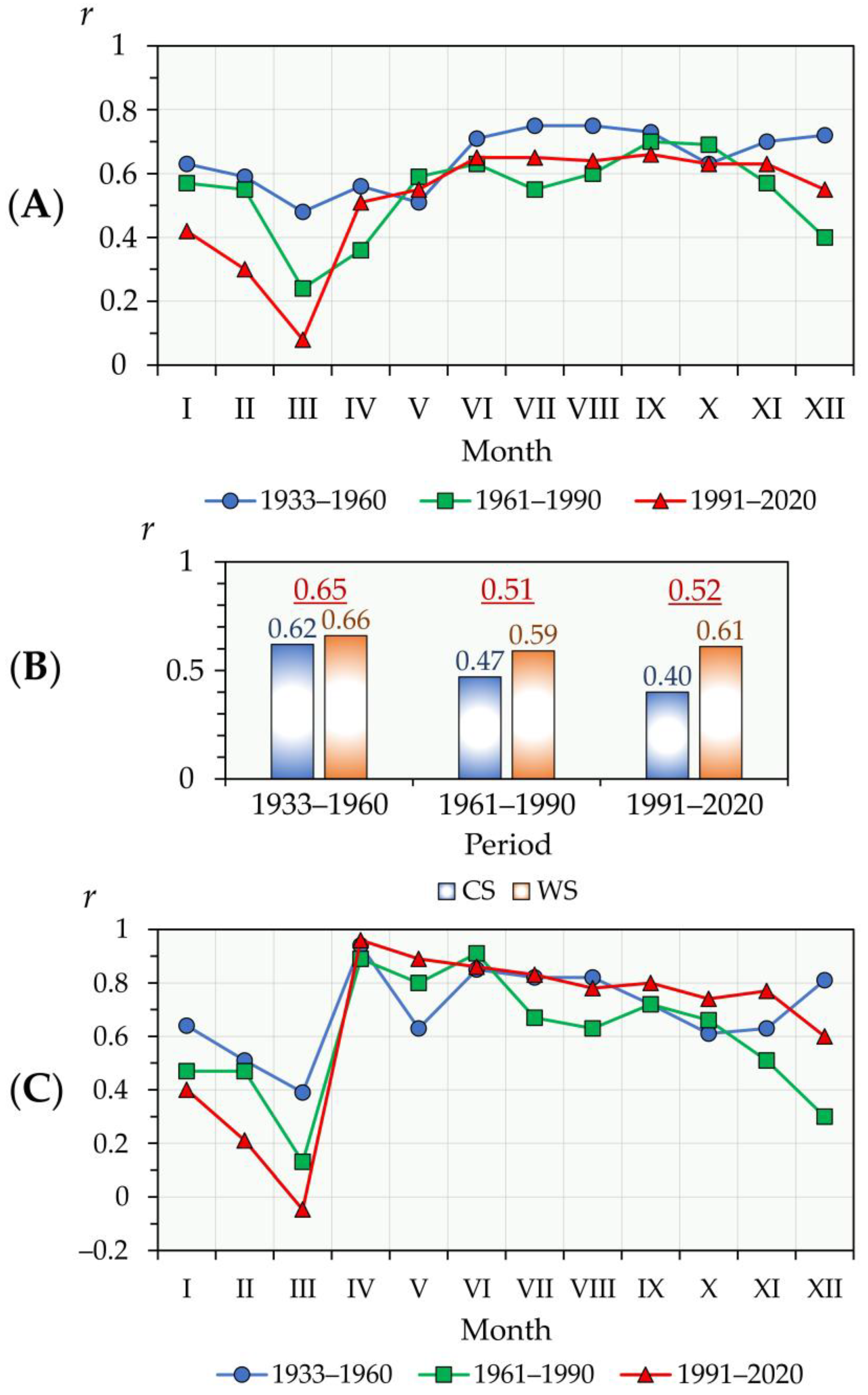
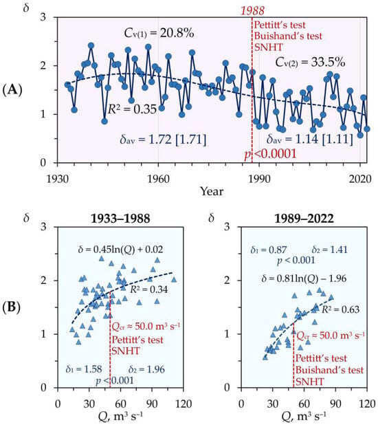
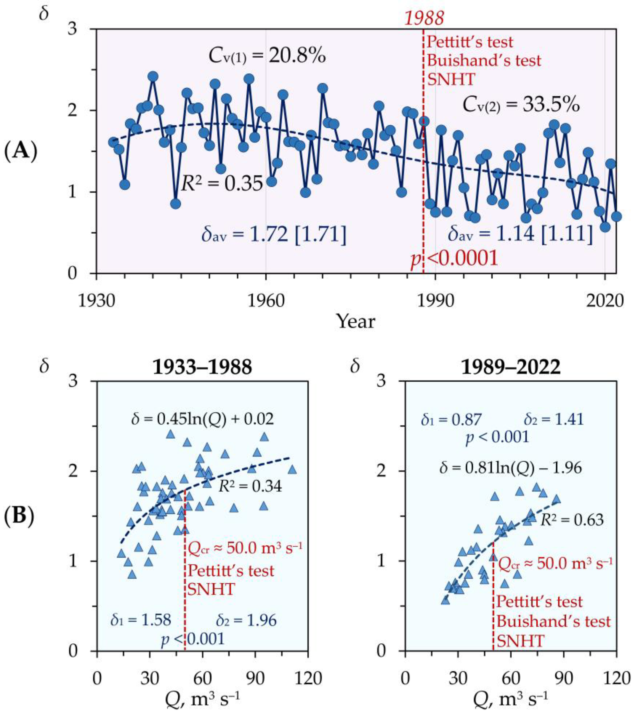
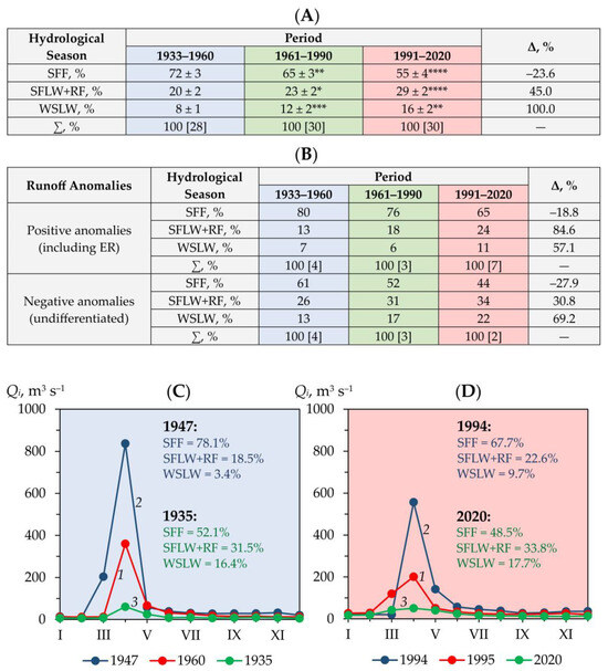
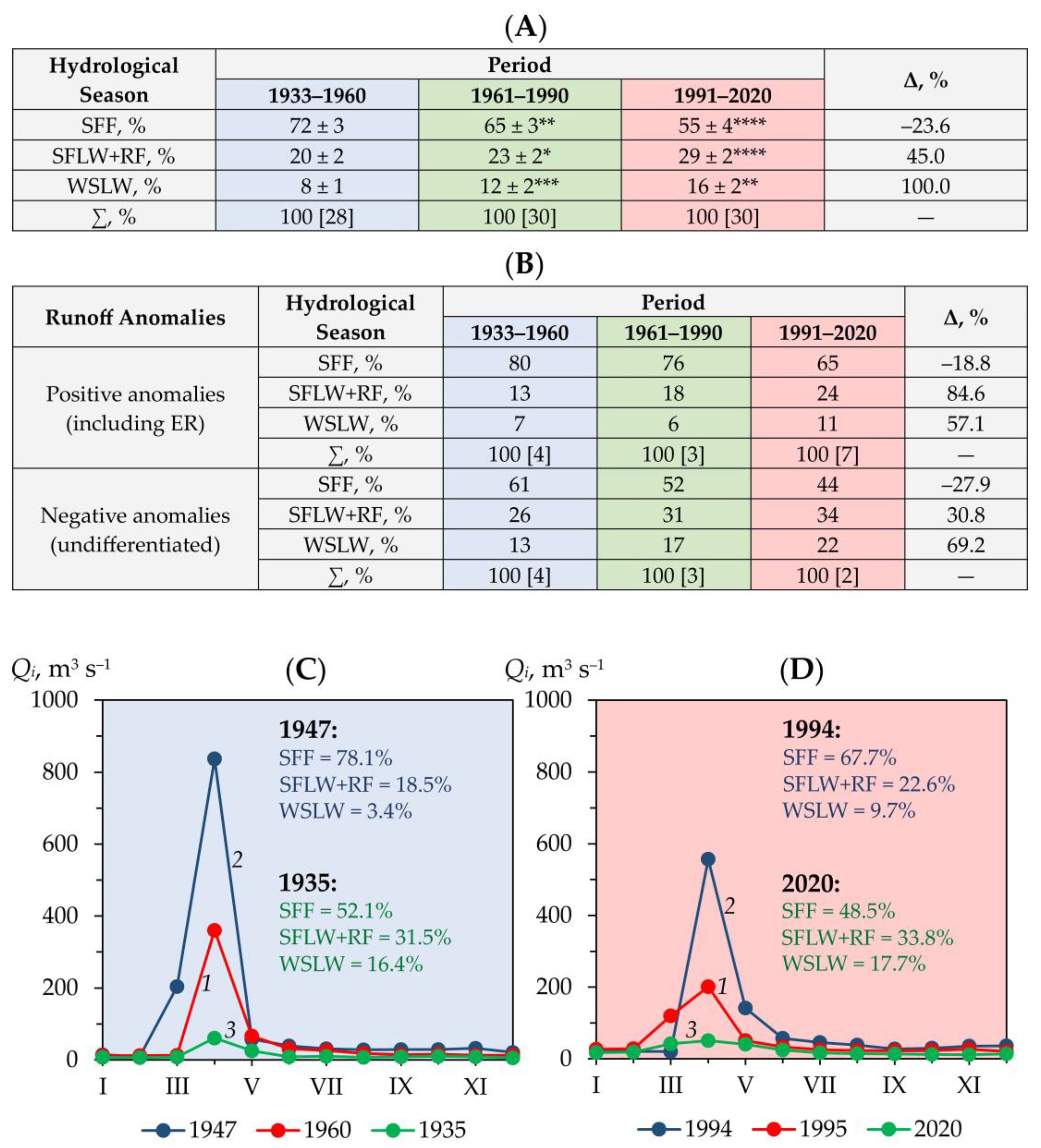
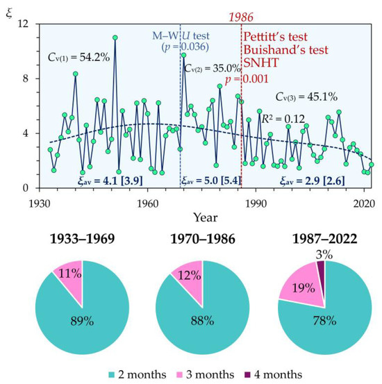
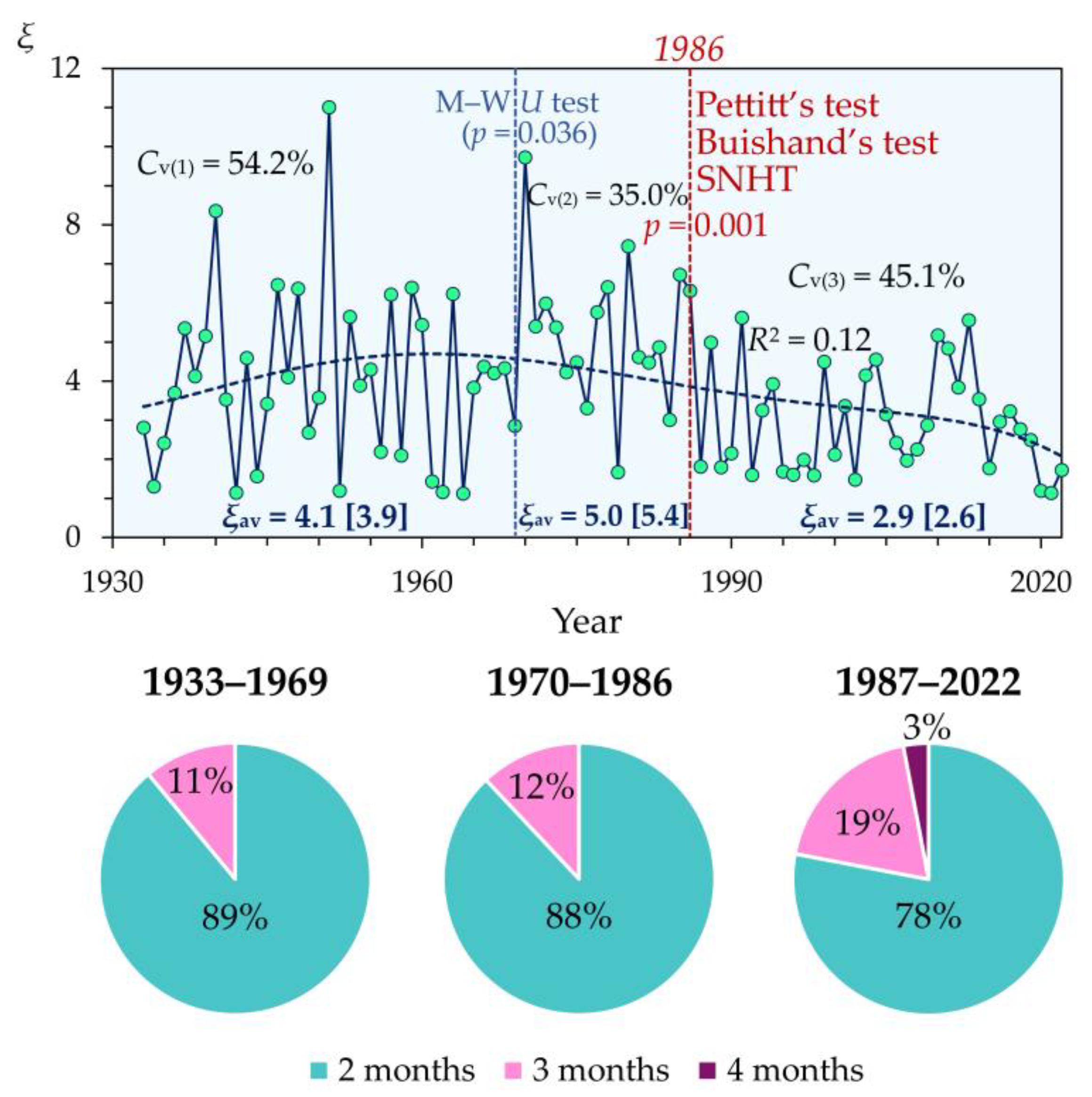
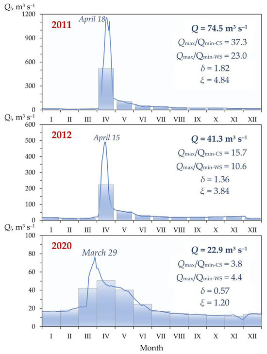
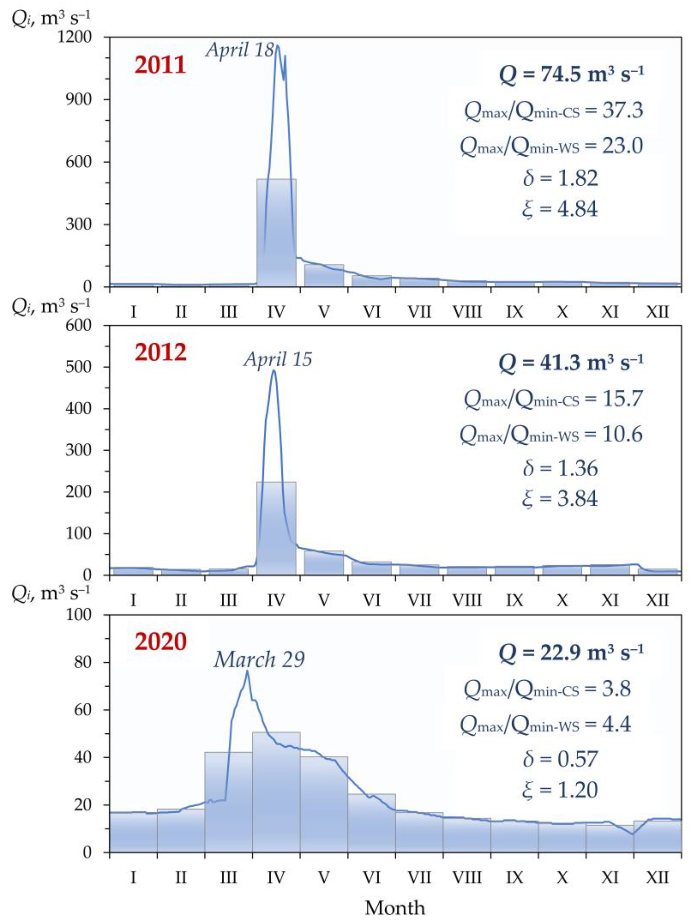
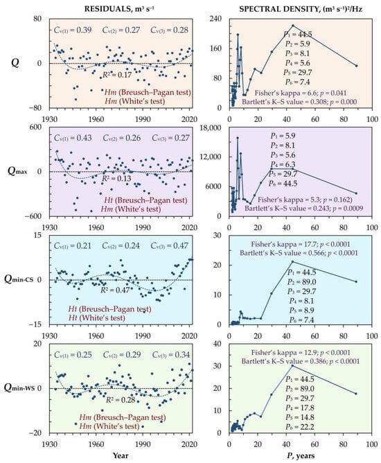
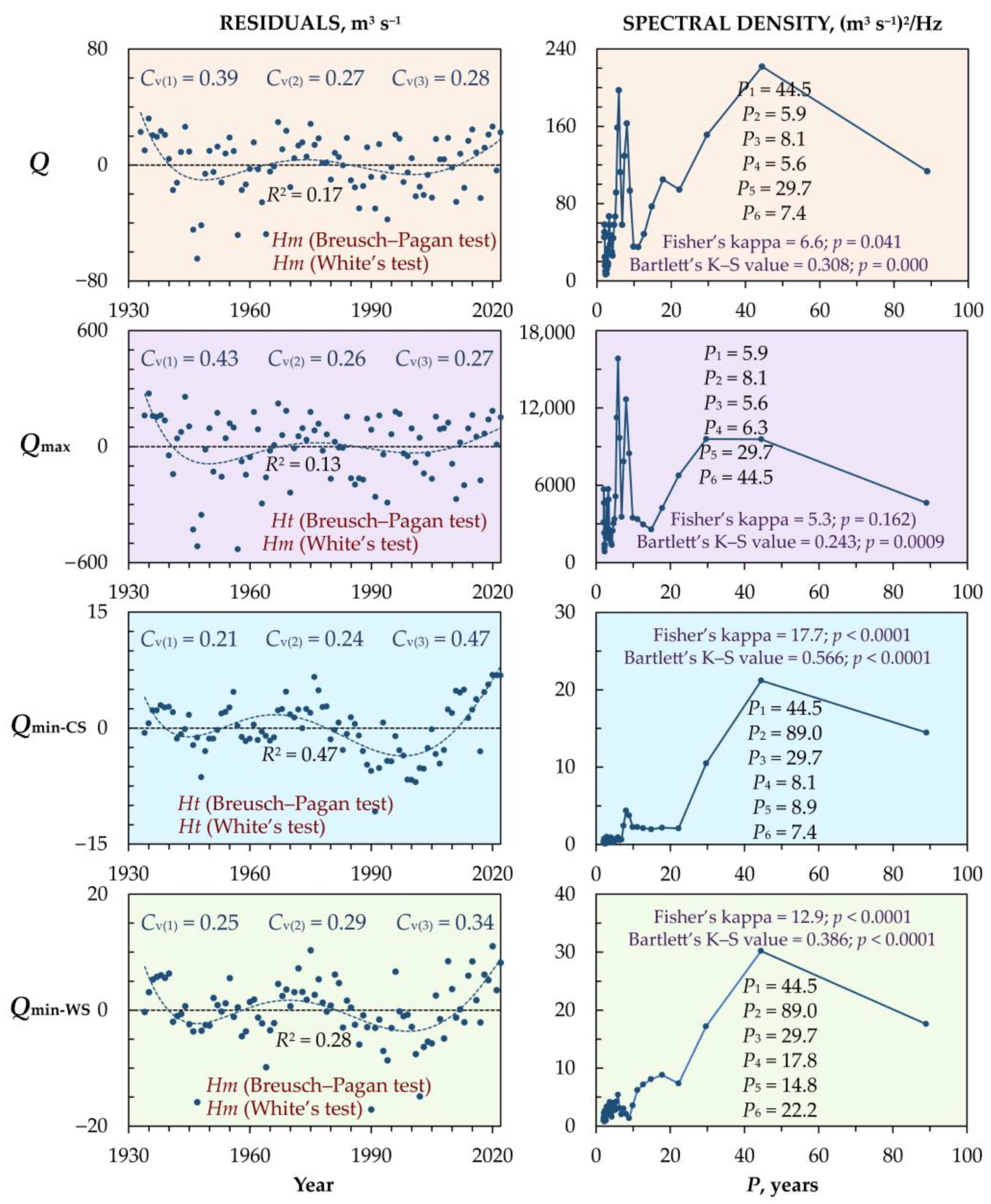
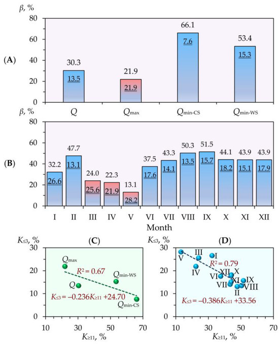
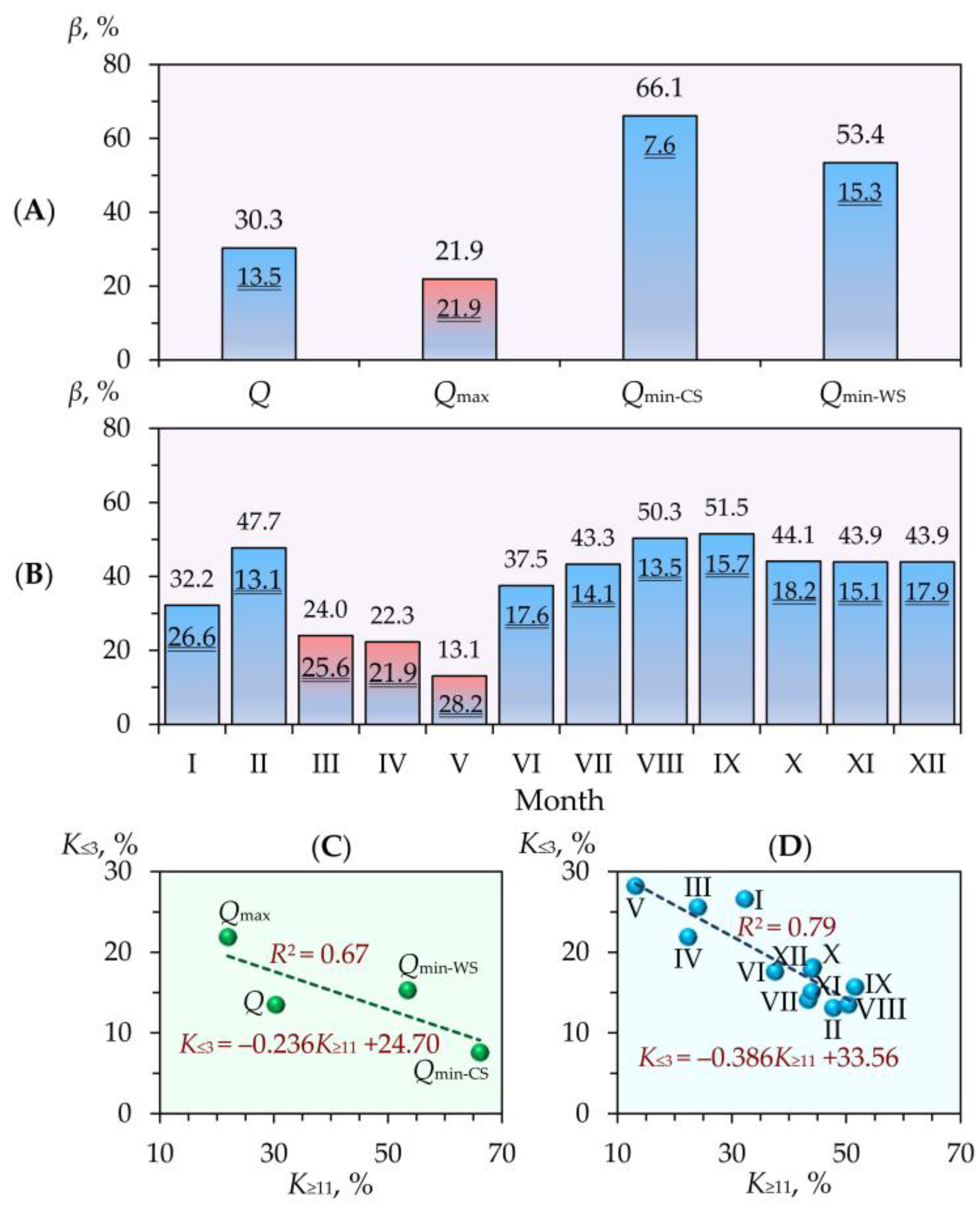
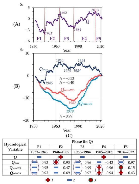
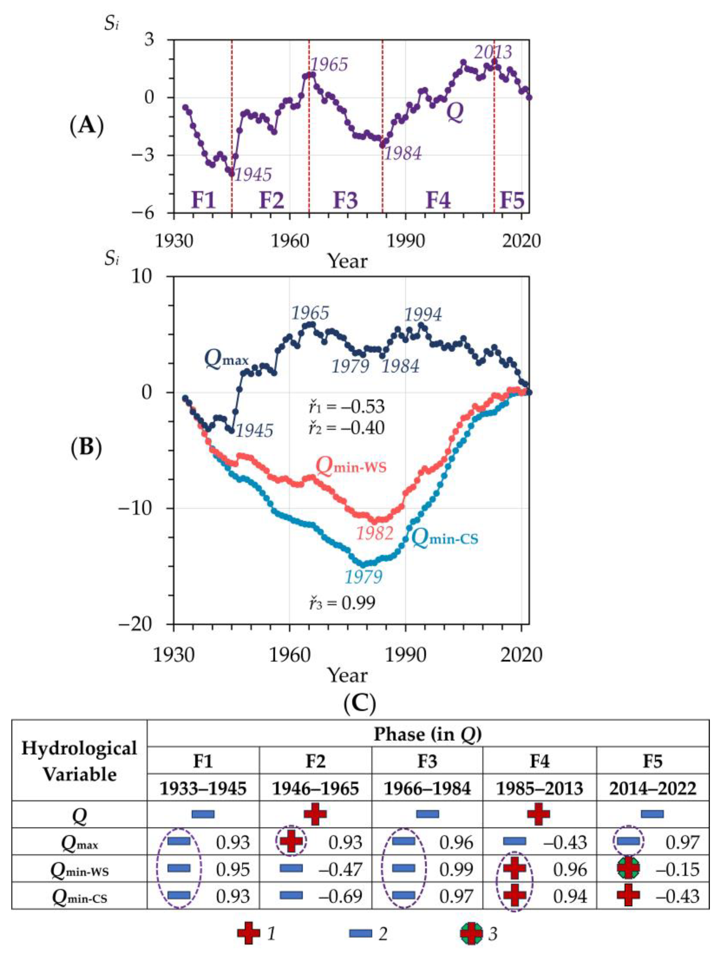

Disclaimer/Publisher’s Note: The statements, opinions and data contained in all publications are solely those of the individual author(s) and contributor(s) and not of MDPI and/or the editor(s). MDPI and/or the editor(s) disclaim responsibility for any injury to people or property resulting from any ideas, methods, instructions or products referred to in the content. |
© 2026 by the authors. Licensee MDPI, Basel, Switzerland. This article is an open access article distributed under the terms and conditions of the Creative Commons Attribution (CC BY) license.