


Abstract
Subsurface freshwater in oceanic islands is typically shaped like a thin lens due to limited land area and recharge, often the primary freshwater source for local communities and highly vulnerable to seawater intrusion (SWI). Saltwater abstraction (SA) is considered as a feasible strategy for mitigating SWI. However, its transient effectiveness for freshwater lens (FWL) development and SWI mitigation in island aquifers, and how the design parameters like SA depth, intensity, and duration affect its performance, remain poorly understood. Therefore, this study employs a two-dimensional, variable-density island groundwater model to simulate the transient responses of FWL development and SWI mitigation to various SA patterns. Six indicators are developed for comprehensive evaluation, including: (1) freshwater recovery efficiency, and the relative changes in (2) average water table elevation (WTE), (3) WTE at the SA well, (4) FWL depth, (5) fresh groundwater volume, and (6) total aquifer salt mass. Simulation results highlight SA depth as the primary determinant of its effectiveness, characterized by critical thresholds that dictate whether SA imposes net positive or negative effects on FWL depth, volume, and aquifer desalinization, with SA intensity and duration serving as scaling factors that amplify the magnitude of these responses. Moreover, while SA can effectively expand FWL volume and shift it toward a more favorable hydrodynamic equilibrium, the diminishing marginal benefits over time cause the FRE to approach zero, indicating SA is a potent short-term restoration strategy rather than a long-term solution from a cost–benefit perspective.
1. Introduction
Seawater intrusion (SWI) represents a process of subsurface freshwater–seawater interface migrating landward and the subsequent salinization of coastal aquifers. It is widely acknowledged that SWI is driven by excessive groundwater extraction and/or climate change, which results in a decrease in the hydraulic gradient between seaward-discharging freshwater and landward-moving seawater [1]. It endangers coastal aquifer ecosystems and restricts subsurface freshwater access for local communities [2,3]. Island aquifers, different from terrestrial coastal aquifers, are primarily recharged by precipitation, including both direct infiltration and indirect contributions from surface water features associated with rainfall (e.g., ponds, wetlands, and ephemeral runoff), forming lens-shaped freshwater bodies atop denser seawater (Figure 1a) [4]. These freshwater lenses are typically thin, commonly on the order of a few meters to several tens of meters in thickness at their maximum, due to the limited land area, low recharge rates, and/or high hydraulic conductivity [5,6], which restrict water accumulation. Therefore, the freshwater lens (FWL) is highly vulnerable to SWI. For many island communities, freshwater aquifers are the sole accessible and economically viable source of freshwater [7,8], so that protecting these critical subsurface resources from SWI is important.
Figure 1.
(a) Cross-section diagram of a FWL in an island aquifer. Key parameters include water table elevation (WTE) and FWL depth (d). (b) An illustration of a saltwater-extraction hydraulic barrier placed in the coastal aquifer. Black dashed and solid lines represent the water table position before and after the barrier implementation, respectively; blue dashed and solid lines represent the freshwater–saltwater interface before and after implementing the hydraulic barrier, respectively.
Within the portfolio of SWI corrective measures, the saltwater abstraction (SA) strategy, commonly referred to as the negative or extraction hydraulic barrier [9,10]. SA functions by extracting saline or brackish groundwater from beneath the freshwater–saltwater interface, thereby creating a localized low-pressure zone within the saline wedge. This pressure reduction diminishes the landward hydraulic gradient of the seawater, allowing the overlying freshwater to vertically expand downward and displace the saltwater seaward. By intercepting the intruding saltwater before it migrates further inland, SA shifts the flow stagnation point toward the coast and stabilizes the freshwater–saltwater interface at a greater depth (Figure 1b). In its barrier form, a line of extraction wells is installed near the shoreline, aligned parallel to the coast and perpendicular to the natural groundwater flow, intercepting saline inflow before it advances inland. Compared with positive hydraulic barriers, which rely on artificial recharge to raise the water table and push back the saline wedge, SA is particularly advantageous in regions where surface water resources for artificial recharge are scarce or where raising the water table is undesirable due to potential surface flooding or land stability concerns.
Early mathematical analyses demonstrated that intensifying SA lowers the freshwater–saltwater interface and forces it to retreat seaward, steepening the interface slope, a finding later confirmed through experimental verification [11]. Recently, with advances in computational modeling, diverse numerical simulations have been conducted to verify the effectiveness of the SA strategy in hindering SWI. For example, Sherif and Hamza [12] and Kacimov et al. [13] applied finite element models to assess salinity distribution in anisotropic coastal aquifers with and without SA. Both studies confirmed that pumping from the freshwater–saltwater transition zone drives the saltwater wedge seaward. Sherif and Hamza [12] highlighted that compared with high equi-concentration lines (10 g/L and above), low equi-concentration lines (4 g/L and below) are more sensitive to SA, shifting seaward noticeably. In real-world applications, Sowe et al. [14] modeled the Wadi Ham aquifer in the UAE using FEFLOW and demonstrated that installing 16 brackish water wells at 1–1.5 km from the shoreline and extracting 44% of the current pumping volume significantly improved groundwater quality by shifting concentration isolines seaward.
The effectiveness of SA systems in mitigating SWI is highly sensitive to design parameters, including SA rates, depth, horizontal distance from the shoreline, and the number and spacing of SA wells. For example, increasing the volume of saline water abstraction generally enhances the efficiency of SA systems in controlling SWI [13,15], but this benefit diminishes beyond a certain SA rate, suggesting the existence of an optimal abstraction intensity, above which additional extraction yields only marginal reductions in SWI length [16]. Mahesha [16] showed that positioning SA wells farther inland can initially improve barrier performance but eventually increases the risk of freshwater being pumped, with the optimal location estimated at around 0.2 times the original wedge toe length from the shoreline. Ebeling et al. [17] found that installing wells slightly landward also offers the advantage of accelerating aquifer remediation, reducing both SWI extent and salt mass on shorter timescales. Moreover, while some researchers have utilized SA wells that fully penetrate the aquifer [16,18], Rastogi et al. [19] found that extending SA depth to the aquifer basement in nearshore regions yields diminishing returns for SWI retardation. Consequently, they suggested that from the perspective of economic cost, a bit shorter wells are preferable in that case. Regarding the effects of the number and spacing of SA wells, Park et al. [18] showed that, given a SA rate, increasing the number of wells can unintentionally induce more saline water toward freshwater wells, reducing overall protection effectiveness; and Mahesha [16] found that wider spacing between SA wells sharply lowers the barrier efficiency, suggesting that optimal SWI mitigation requires that SA well spacing is lower than 5% of the initial saltwater wedge toe length.
Despite its potential, the SA strategy has been studied almost exclusively in the context of terrestrial coastal aquifers. In continental coastal aquifers, SWI typically develops as a laterally advancing saline wedge, but island aquifers are characterized by vertically stratified FWLs floating atop denser seawater under near-hydrostatic equilibrium. In continental systems, SA primarily alters the horizontal position and slope of the saline wedge, with system evolution dominated by lateral displacement processes, whereas the island aquifers’ response to SA is largely governed by vertical redistribution of freshwater and saltwater, including suppression of saltwater upconing and changes in FWL thickness. Moreover, the limited spatial extent and storage capacity of island aquifers may result in shorter response times and stronger coupling between recharge, abstraction, and density-driven flow. Therefore, the transient behavior of FWLs under SA cannot be directly inferred from studies of continental saline wedges, necessitating a dedicated investigation into island hydrogeological settings.
To date, SA has received limited attention as a strategy for FWL development and SWI mitigation in oceanic island environments. A recent investigation of Yu et al. [20] demonstrated that, under the same SA intensity and pumping depth, locating the SA well closer to the island center is more effective than nearshore placement, resulting in larger increases in subsurface freshwater storage and greater reductions in aquifer salt mass. However, to the best of the authors’ knowledge, no studies have yet systematically explored the temporal effects of the SA strategy on FWL dynamics and the SWI extents in island aquifers, nor have they investigated how different SA patterns affect the transient behaviors of FWL and SWI extent.
Motivated by these, this study aims to investigate the temporal performance of SA in FWL development and SWI mitigation in unconfined island aquifers, and explore how the design parameters, such as SA depth, intensity, and duration, affect its effectiveness. This investigation employs a simplified two-dimensional (2D), variable-density, dispersive, island aquifer simulation model based on hydrogeological conditions observed in the island aquifer of San Salvador Island, Bahamas. It focuses on a single-well problem, with the SA well positioned at the island’s geographic center. Specifically, a predefined set of SWI simulation scenarios is designed to quantify the impact of the SA depth, intensity, and duration on average water table elevation (WTE), drawdown at the pumping well, FWL depth, subsurface freshwater volume, freshwater recovery efficiency (FRE), and aquifer salt mass. These simulations are conducted using the MODFLOW family SEAWAT model to capture the complex, time-dependent interactions between the SA activity and the island groundwater system.
2. Methodology
2.1. Study Area: San Salvador Island
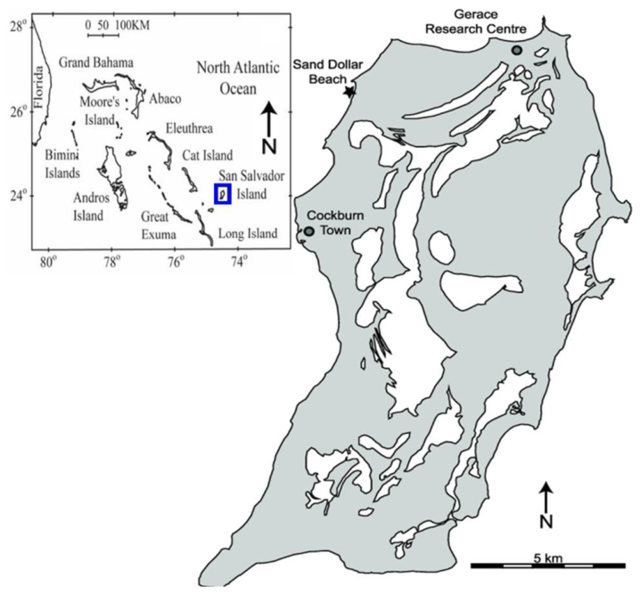
This study investigates the temporal influence of SA on FWL development and SWI mitigation in unconfined island aquifers. Using the San Salvador Island aquifer as a case study, it evaluates how various SA patterns influence the transient behaviors of FWL and SWI extents. San Salvador Island is an isolated carbonate platform located within the Bahamian Archipelago, approximately 600 km east-southeast of Miami (Figure 2) [21,22]. It is characterized as a strip island, spanning roughly 20 km along its north-south axis with an average east–west width of 8 km [23].
The local topography is dominated by consolidated carbonate dune ridges with elevations typically reaching several meters above sea level [24]. Under a subtropical climate, the island experiences annual temperatures between 22 and 28 °C [22]. Hydrologically, the region is characterized by annual precipitation ranging from 1000 to 1250 mm/year, while potential evaporation typically exceeds input at 1250 to 1375 mm/year [25].
Figure 2.
Location map of San Salvador Island [25]. The gray and the white areas represent land and surface water, respectively.
2.2. Development of Numerical Simulation Model for SWI
This study employs the SEAWAT code to simulate the transient dynamics of FWL evolution and SWI in an unconfined island aquifer under SA. SEAWAT integrates MODFLOW (groundwater flow) and MT3DMS (solute transport) to solve the variable-density flow equations via a finite-difference numerical approach [26]. The governing flow equation is formulated in terms of equivalent freshwater head, accounting for fluid density variations as a function of salt concentration. This mathematical framework is particularly well suited for simulating the complex freshwater–seawater interactions inherent in island hydrogeological settings. Detailed descriptions of the governing equations for groundwater flow and solute transport are provided by [26].
To efficiently evaluate the temporal performance of various SA strategies in FWL development and SWI mitigation in San Salvador Island, a simplified 2D, variable-density, dispersive, vertical ‘cross-section’ model is adopted, representing an idealized North-South transect across the long width of the island. This modeling approach is appropriate for a strip-island setting, where the island extends laterally with relatively uniform hydrogeological conditions along its length, and the dominant groundwater flow and density-driven processes occur primarily in the vertical plane perpendicular to the coastline. Under such conditions, the essential dynamics of FWL and SWI under SA can be effectively captured within a cross-sectional framework.
Figure 3 illustrates the conceptual model domain, including the numerical discretization and assigned boundary conditions. This 2D cross-section model represents a homogeneous, isotropic, unconfined island aquifer as a rectangular domain with a length of 2000 m, a height of 116 m, and a width of 1 m. The domain is discretized using a finite-difference grid with a uniform lateral resolution of 2 m. Vertically, the grid employs a 2 m cell height for the top layer to accommodate water table fluctuations, while the remaining layers maintain a 1 m resolution. To implement the lateral boundary conditions, two additional columns are included at the domain’s extremities. The resulting numerical mesh consists of 1002 columns and 115 layers, totaling 115,230 cells.
Figure 3.
Island aquifer SEAWAT cross-sectional model grid, along with the associated boundary conditions and the placement of the SA well.
A no-flow boundary is applied at the base of the aquifer. The upper boundary is defined by a specified flux (Neumann) condition representing effective aquifer recharge (RCH). To reflect long-term average hydrological conditions, RCH is assumed to be spatially uniform and constant over time for each simulation. RCH is assigned a salt concentration of 0.0 g/L, representing pure freshwater input at the land surface. The lateral boundaries (left and right) are defined by a constant head (Dirichlet) boundary with head () of 0.0 m to represent sea level at the datum, with a constant seawater concentration (C) of 35.0 g/L. These constant head and concentration conditions effectively represent the hydraulic connection between the aquifer and the surrounding ocean under quasi-steady sea-level conditions. Moreover, to evaluate the first-order dynamics of the FWL and SWI, the aquifer system of San Salvador Island, predominantly composed of carbonate materials, is conceptualized as a homogeneous and isotropic porous medium, and is assigned a high hydraulic conductivity (HK) of 50.0 m/day, representing the primary flow characteristics of the island’s carbonate matrix. The SA system is represented by a point sink located at the island center at a specified depth (D). The extraction rate (Q) represents the volume of brackish or saline water removed per unit time and per unit aquifer width.
The simulation of island groundwater flow and solute transport under various SA strategies is divided into two distinct stress periods. The first stress period aims to establish steady-state FWL and SWI extents under conditions of RCH and the prescribed boundary conditions. This phase is executed until the hydraulic head and concentration fields reach a state of dynamic equilibrium, providing a robust initial condition for the subsequent phase. The second stress period simulates the transient aquifer response to SA over the specified management horizon. The total simulation duration is calculated based on the SA period (in years) using a conversion of 360 days per year. To capture the transient evolution of hydraulic and transport processes, this period is discretized into uniform 30-day time steps. The groundwater flow equation is solved using the Preconditioned Conjugate Gradient solver, with both head-change convergence criterion and residual convergence criterion set to 1 × 10⁻⁵, and Solute transport was solved using the Generalized Conjugate Gradient package within MT3DMS, with a relative concentration convergence criterion of 1 × 10⁻⁶. These solver tolerances were selected to ensure numerical stability and solution accuracy for density-dependent flow conditions. Table 1 provides a list of the relevant parameters adopted in the simulation model introduced above. These parameters are based on published case studies [27,28,29] of island aquifers in the Bahamian archipelago.
Table 1.
Model parameters used for SWI Simulation in the 2D island aquifer model.
This 2D cross-sectional model can capture the fundamental physics of density-driven flow and FWL dynamics under SA, though it assumes homogeneous and isotropic aquifer conditions. In reality, carbonate island aquifers such as San Salvador Island often exhibit significant geological heterogeneity due to karstification, including dissolution conduits, fractures, and high-permeability preferential flow paths. These heterogeneities influence SWI processes by enhancing hydraulic connectivity, accelerating saltwater upconing, and modifying the spatial distribution of groundwater salt concentration. However, a 2D simplified model is intentionally adopted in this study for the following reasons: (1) to isolate the influence of SA design parameters from the confounding effects of complex karst-influenced hydrogeological structures; (2) to establish a primary benchmark for investigating fundamental transient behaviors of FWL and SWI under SA in strip-island settings; and (3) to ensure computational efficiency and feasibility within the scope of this study.
2.3. SWI Simulation Scenarios
This work employs SEAWAT simulations to investigate how FWL and SWI extent in unconfined island aquifers respond to SA over time, with a focus on the influence of SA patterns on this response. Herein, SA patterns are defined by three primary decision variables (DVs): the depth D [L] at which pumping occurs, the intensity of constant pumping Q [L2T−1], and the pumping duration t [T]. As the SA strategy involves positioning the well screen within the freshwater–saltwater mixing zone or the underlying saltwater zone, the pumping depth is defined as the vertical distance between the well location and the FWL bottom for analytical convenience, denoted by . A positive indicates that the well is located below the FWL bottom; for example, = 1 m corresponds to a well position 1 m beneath the FWL bottom. Inherently, numerous SWI simulations need to be conducted, with these three independent DVs, , Q, and t, being varied continuously. Due to the computational demands of simulating these continuous variables, the investigation utilizes a prescribed ensemble of simulation scenarios to promote efficiency. By evaluating differences in WTE, FWL geometry, freshwater storage, and overall aquifer salinization, this work establishes a robust framework for drawing general conclusions on the transient responses of island aquifers to various SA patterns.
Table 2 provides a description of the ensemble of DV sets (, Q, t) used in this study. In this work, eight values of are considered (1, 2, 4, 6, 8, 10, 12, and 15 m). Based on the steady-state baseline simulation, the corresponding initial groundwater salt concentration at these depths is 1.17, 2.71, 11.64, 24.29, 29.19, 31.50, 32.69, and 33.62 g/L, respectively. These values indicate that the selected SA depths span a wide range from the freshwater–saltwater transition zone (brackish) to fully saline regions, allowing for an investigation into how vertical SA positioning influences FWL dynamics and SWI control. Pumping intensity Q is evaluated at six levels, proportional to the total island recharge (RCH∙L): 0.05 RCH∙L, 0.1 RCH∙L, 0.2 RCH∙L, 0.4 RCH∙L, 0.6 RCH∙L, and 0.8 RCH∙L. The SA strategy is evaluated over four management horizons (t): 5, 10, 25, and 50 years.
Table 2.
Values of DVs (decision variables) considered for the SA strategies.
A full-factorial combination of these DV values leads to an ensemble of 8 × 6 × 4 = 192 alternative SA strategies, and thus as many SEAWAT model runs. An additional model run is also needed to simulate the baseline “no-SA” scenario.
2.4. Indicators for Quantifying FWL Dynamics and SWI Extent
This study formulates six indicators to systematically evaluate the impact of SA patterns on the transient behaviors of FWL and SWI extent, including (1) relative change in average WTE (); (2) relative change in the WTE over the pumping well (); (3) relative change in FWL depth (); (4) relative change in fresh groundwater volume (); (5) the ratio of the net increase in subsurface freshwater storage to the total volume of extracted saltwater (FRE); and (6) relative change in total aquifer salt mass () [30]. Indicators and provide normalized measures of the overall water table shift and the peak water level fluctuations across different SA scenarios, respectively. To track FWL morphology, is used to quantify the deepening or shallowing of the freshwater–saltwater interface under SA. and assess the degree of SWI mitigation by quantifying changes in subsurface freshwater storage and total salt mass, respectively. FRE is employed to quantify the efficiency of implementing SA in promoting freshwater storage. These indicator values at a specific management horizon t are given by the following equations,
where , , , , , and represent , , , , FRE, and at the management horizon t, respectively; and denote the average WTE before SA and at a given duration t of SA, respectively; and are the initial WTE at the island center before SA and WTE over the SA well at a given duration t of SA, respectively; and represent the initial FWL depth at the island center before SA and FWL depth at the island center under a given duration t of SA, respectively; and denote the initial freshwater volume before SA and the subsurface freshwater volume under a given duration t of SA, respectively; is the total volume of extracted saltwater until the end of the management horizon ; and are the total aquifer salt mass before SA and under a given duration t of SA, respectively.
The average WTE is calculated by integrating the water table elevations across all top-layer island aquifer cells and then dividing by the number of these grid cells. All WTE values correspond to equivalent freshwater head values derived directly from the model output, without requiring additional density correction. The FWL depth is defined as the distance from the freshwater–saltwater interface at the island center to the datum (see Figure 1a). Groundwater with a salt concentration of 1.0 g/L or less is defined as freshwater, and this threshold is a common convention in island hydrogeology and numerical modeling of the freshwater–saltwater interface, which can effectively represent the transition between potable fresh groundwater and the brackish mixing zone [20]. Similarly, subsurface freshwater volume is calculated by spatial integration of the pore volume in those grid cells where the simulated salt concentration is no more than 1.0 g/L. Total aquifer salt mass are identified by integrating the salt concentration multiplied by the pore volume over all model grid cells. In summary, for the defined indicators, positive values of , , , , and denote a decline in average WTE, a decline in WTE at the SA well, an increase in FWL depth, an expansion of freshwater volume, and an increase in total aquifer salt mass, respectively, while negative values represent their opposite trends.
3. Results and Discussion
3.1. FWL and SWI Extent Prior to the SA Implementation
The steady-state groundwater concentration distribution for the baseline scenario prior to SA implementation is depicted in Figure 4. Under the natural condition, FWL depth varies from zero in proximity of the shoreline to about 26 m relative to the datum at the island center. The corresponding depth to the seawater increases from about 10 m near the coast to roughly 60 m at the island center. It indicates that the freshwater–saltwater mixing zone gradually widens from the shoreline to the island center, in agreement with theoretical predictions [31].
Figure 4.
Groundwater concentration distribution at the steady state in the baseline scenario. The red dashed line represents the 1.0 g/L concentration contour, delineating the freshwater–saltwater transition zone, while the black dashed line indicates the 35.0 g/L contour, approximating the seawater boundary.
Table 3 shows a summary of initial indicator values for the island aquifer at the baseline case. These reference values are provided to facilitate interpretation of the relative change plots by establishing a consistent benchmark against which scenario-based deviations can be quantitatively evaluated.
Table 3.
Summary of initial indicator values for the island aquifer at the baseline case.
The simulated results of and at the baseline case show close agreement with the corresponding estimates according to the established theoretical solutions [5,6,32], and visually, the freshwater–saltwater mixing zones in Figure 4 gradually widen from the shoreline to the island center, in agreement with theoretical predictions [31], thereby validating the developed model’s accuracy. These robust validations highlight this model’s reliability for subsequent investigations on the transient response of the island groundwater system to various SA patterns.
3.2. Transient Responses of WTE Indicators to Various SA Patterns
Figure 5 shows the transient response of to various SA patterns across four management horizons, from t = 5 to 50 years. Each panel displays as a function of the relative SA depth , with separate profiles representing different Q levels. In Figure 5, values for all for all SA patterns remain positive and exhibit a non-linear decreasing behavior with increasing, a trend significantly more pronounced under high-Q strategies or extended management horizons. For any given , values under higher Q are larger than those under SA patterns with lower Q, and this gap is more evident at shallower positions, while less remarkable with the pumping location moving deeper. Moreover, over time, values show two distinct depth-dependent behaviors, continuously growing at 8 m while decreasing in the case of > 8 m; and the gap in values between different Q levels at shallower positions remains significant from t = 5 to 50 years, but this gap at > 8 m gradually diminishes between t = 5 and 25 years, reaching a stabilized state by t = 50 years.
Figure 5.
Profiles of the indicator (relative change in average WTE) for various SA patterns at four management horizons: (a) 5 years, (b) 10 years, (c) 25 years, and (d) 50 years. Profile legends are provided at the bottom of the figure.
The observations in Figure 5 reveal that: (1) within the predefined range of depths, SA inevitably induces water table drawdown at the pumping well, which is significantly amplified by higher Q and/or utilizing shallower pumping positions; (2) adopting deeper SA patterns can gradually diminish the impact of SA on water table and decrease the magnitude of the average aquifer drawdown, as deeper SA effectively decouples the hydraulic stress from the water table. It can be inferred that when the pumping location is sufficiently deep, the influence on water table drawdown may become negligible; (3) SA depths play an important role in determining the temporal evolution of average water table drawdown, characterized by a distinct critical depth threshold. SA at depths shallower than that threshold tends to increase average water table drawdown over time, due to the continuously unintended extraction of freshwater, while conversely, SA beyond that threshold can actually alleviate drawdown over time, which effectively intercepts and abstracts upconing saltwater, allowing for a more favorable pressure distribution and FWL expansion. Both the temporal increase and decrease in drawdown eventually reach a quasi-steady state as the system moves towards equilibrium over a long-term management horizon.
Figure 6 displays the transient response of to various SA patterns across the same management horizons, from t = 5 to 50 years. Each panel displays as a function of the relative SA depth , with separate profiles representing different Q levels. It is clear to observe that the behavior of closely mirrors that of (Figure 5), with all values remaining positive and exhibiting a non-linear decrease as increases; furthermore, high-Q patterns consistently result in larger values than low-Q scenarios, displaying greater sensitivity to Q at shallower depths. There also exists a similar critical depth threshold, below which values increase with t while beyond which they decrease with t, and the disparities in values between different Q conditions eventually tend toward stabilization with t.
Figure 6.
Profiles of the indicator (relative change in the WTE over the SA well) for various SA patterns at four management horizons: (a) 5 years, (b) 10 years, (c) 25 years, and (d) 50 years. Profile legends are provided at the bottom of the figure.
Despite the similarities in their transient behavior, Figure 5 and Figure 6 reveal four key distinctions between the responses of and to various SA patterns, including: (1) For any SA patterns, their values are consistently greater than the corresponding values, indicating SA induces a more pronounced decline in WTE over the pumping well compared with the average WTE decline across the entire aquifer. (2) With increasing, the discrepancy between and gradually diminishes. Taking Q = 0.8 RCH∙L and t = 5 years as an example, the difference between and declines from 10.39% at = 1 m to 9.11% at = 2 m, and to just 1.01% at = 15 m; and in the case of Q = 0.4 RCH∙L and t = 10 years, the difference between and declines from 6.50% at = 1 m to 5.60% at = 2 m, and to just 0.32% at = 15 m. (3) With the management horizon t extending, the discrepancy between and gradually decreases before reaching a stable state. For example, at Q = 0.6 RCH∙L and = 1 m, the difference between and drops from 8.80% at t = 5 years to 8.02% at t = 10 years, and to 6.44% at t = 25 years, and to 6.15% at t = 50 years; at Q = 0.8 RCH∙L and = 1 m, the difference between and declines from 10.39% at t = 5 years to 9.17% at t = 10 years, and to 7.30% at t = 25 years, and to 6.98% at t = 50 years. (4) The disparities in across different Q levels are more pronounced than the corresponding disparities observed in , indicating that Q exerts a more significant influence on drawdown at the SA well than on the average WTE drawdown. For example, at = 1 m and t = 5 years, the difference in between Q = 0.2 RCH∙L and Q = 0.4 RCH∙L is 5.79%, while the corresponding difference in is 2.96%; the difference in between Q = 0.6 RCH∙L and Q = 0.8 RCH∙L is 3.87%, while the corresponding difference in is 2.28%.
The discrepancy between and is primarily driven by the formation of a cone of depression, where groundwater is removed from the immediate vicinity of the SA well faster than it can be replenished by surrounding groundwater flow, thereby creating a steep hydraulic gradient and a localized sink where the WTE reaches its lowest point at the SA well. In contrast, since the hydraulic impact of pumping on WTE diminishes with distance from the well, the regional WTE remains higher than the level at the extraction point, resulting in a significantly smaller decline in average WTE. The discrepancy between and is most acute at shallow SA depths and high intensities, as the pumping stress is concentrated near the phreatic surface, making the WTE over the SA well highly sensitive to changes in Q. However, as SA depth increases, the vertical distance from the water table provides a hydraulic buffer that dissipates pressure more uniformly, causing the localized sink to flatten and the two WTE indicators to converge. It should be noted that the magnitude and spatial distribution of water table drawdown are also influenced by the assumed isotropic HK in the model. Under isotropic conditions, flow toward the pumping well is symmetrically distributed, leading to a pronounced localized decline in WTE relative to the aquifer-wide average. In anisotropic or heterogeneous systems, where HK varies with direction or spatially, the drawdown pattern may become asymmetric due to preferential flow pathways or differences in horizontal and vertical flow resistance. These factors may alter the magnitude of both and , although the general tendency for more significant drawdown near the pumping well is expected to remain. Over time, the system transitions from an initial high-pressure shock toward a quasi-steady state, allowing the aquifer to redistribute pressure and the freshwater lens to expand, which gradually stabilizes the hydraulic gradients and narrows the gap between these two WTE indicators.
In summary, the observations from Figure 5 and Figure 6 reveal the following key insights regarding the transient response of average WTE and WTE at the well to various SA strategies: (1) implementing SA leads to the comparable decreases in both average WTE and WTE at the pumping well, with greater declines in the WTE at the SA well than the average WTE; (2) the discrepancy of declining magnitudes between average WTE and WTE at the SA well tend to gradually narrow with SA depth increasing and/or management horizon extending, eventually reaching a stable, minimized gap; (3) higher-Q SA patterns exacerbate larger declines in both WTE indicators, a trend more evident at the SA well closer to the FWL zone; (4) a distinct depth threshold exists that governs the temporal evolution of drawdown at the well and across the aquifer. In the case of SA at depths shallower than this threshold, both WTE indicators experience intensified declines over time, but conversely, with SA depths beyond this threshold, the declines in both WTE indicators are alleviated over time. Consequently, it can be inferred that the hydraulic impact of SA on the WTE becomes negligible if the SA depth is sufficiently deep, effectively decoupling the pumping stress from the phreatic surface.
3.3. Transient Responses of FWL Depth to Various SA Patterns
Figure 7 shows the transient response of to various SA patterns across four management horizons, from t = 5 to 50 years. Each panel displays as a function of the relative SA depth , with separate profiles representing different Q levels. In Figure 7, the profiles of across all SA patterns exhibit a distinct non-monotonic relationship with , characterized by an initial sharp rise from negative values to a peak positive value, followed by a gradual decline as the SA depth increases further. It is remarkable to observe a consistent critical depth threshold at approximately = 6 m, in which SA exerts a nearly negligible impact on , regardless of Q or t. However, the profiles of diverges sharply on either side of this threshold. Implementing SA at the depths shallower than this threshold consistently yields negative values, indicating an upward shift of the FWL interface and a reduction in FWL depth; and in this shallow regime, higher Q patterns lead to more significantly negative values compared with lower Q patterns. Conversely, implementing SA at depths deeper than this threshold (i.e., further below the FWL bottom within the mixing or saltwater zone) results in positive values, indicating a downward displacement of the FWL interface and an increase in FWL depth; and in this deep regime, higher Q patterns are actually more beneficial, generating increasingly positive values.
Figure 7.
Profiles of the indicator (relative change in the FWL depth) for various SA patterns at four management horizons: (a) 5 years, (b) 10 years, (c) 25 years, and (d) 50 years. Profile legends are provided at the bottom of the figure.
In terms of temporal evolution, values exhibit two distinct stabilization behaviors based on the SA regime. For SA within the shallow regime ( < 6 m), values become increasingly negative over time before reaching a steady state. SA patterns with lower Q and/or locations closer to the critical depth threshold reach stability more rapidly. Notably, nearly all shallow SA configurations achieve a stable state by t = 25 years. For SA within the deep regime ( > 6 m), values trend toward more positive levels as t increases. Similar to the shallow regime, SA patterns with lower Q and/or depths near the 6 m threshold stabilize earlier. While configurations with Q 0.2 RCH∙L generally reach stability by t = 25 years, those with Q > 0.2 RCH∙L continue to show growth in lens expansion (more positive ) even after 50 years.
Within the deep SA regime ( > 6 m), all SA patterns exhibit an optimal depth for reaching the maximum positive values. These optimal depths are not static, evolving based on both t and Q. Specifically, the optimal depths for peak positive values display the following characteristics: (1) the optimal depth generally increases over time before reaching a steady state; (2) higher-Q SA patterns are characterized by deeper optimal depths. For example, the peak positive values under Q = 0.1 RCH∙L remains stable at = 8 m across all time horizons from 5 to 50 years; the optimal depth for maximum values under Q = 0.4 RCH∙L shifts from = 8 m at t = 5, 10 years, eventually stabilizing at = 10 m for the long-term horizons (t = 25 and 50 years); and the peak of under Q = 0.6 RCH∙L progresses from = 8 m at t = 5 years to = 10 m at t = 25 years, finally reaching = 12 m at t = 50 years.
These observations in Figure 7, overall, reveal that the SA depth is a decisive factor in determining the effectiveness of SA for FWL depth expansion, characterized by two distinct depth thresholds. The first threshold serves as a functional pivot point, SA at depths shallower than which SA narrows FWL depth, a degradative trend exacerbated by shallower pumping, and/or higher Q, and/or extending management horizon, whereas SA deeper than which SA contributes to FWL depth downward expansion. The second depth threshold, positioned deeper than the first, is identified as the optimal depth for the SA strategy to achieve the maximum FWL depth. Between these two depth thresholds, the magnitude of FWL depth expansion increases with SA depth before it reaches the peak at this second threshold, and beyond this point, the expansionary benefit gradually diminishes with further increase in SA depth. It can be inferred that the impact of SA on the FWL depth eventually converges to zero at sufficiently large depths, where the SA well becomes hydraulically decoupled from the FWL zone. Notably, this optimal depth is not static, which shifts deeper over time before reaching a stable state, and higher-Q SA patterns consistently require deeper optimal depths than lower-Q ones.
The physical mechanisms behind the above findings are further elucidated by Figure 8, Figure 9 and Figure 10, which show the simulated groundwater flow fields and salt concentration distributions under SA implementation with different combinations of (1, 8, and 15 m) and t (5, 10, 25, and 50 years), for Q = 0.05 RCH∙L, 0.2 RCH∙L, and 0.8 RCH∙L, respectively.
Figure 8.
Groundwater flow fields and salt concentration distributions under SA implementation for Q = 0.05 RCH∙L and different combinations of and t: (a) = 1 m, t = 5 years; (b) = 8 m, t = 5 years; (c) = 15 m, t = 5 years; (d) = 1 m, t = 10 years; (e) = 8 m, t = 10 years; (f) = 15 m, t = 10 years; (g) = 1 m, t = 25 years; (h) = 8 m, t = 25 years; (i) = 15 m, t = 25 years; (j) = 1 m, t = 50 years; (k) = 8 m, t = 50 years; (l) = 15 m, t = 50 years. Red markers denote the SA well. White dashed lines represent the initial FWL boundary before SA, and red dashed lines represent the FWL boundary during SA implementation.
Figure 9.
Groundwater flow fields and salt concentration distributions under SA implementation for Q = 0.2 RCH∙L and different combinations of and t: (a) = 1 m, t = 5 years; (b) = 8 m, t = 5 years; (c) = 15 m, t = 5 years; (d) = 1 m, t = 10 years; (e) = 8 m, t = 10 years; (f) = 15 m, t = 10 years; (g) = 1 m, t = 25 years; (h) = 8 m, t = 25 years; (i) = 15 m, t = 25 years; (j) = 1 m, t = 50 years; (k) = 8 m, t = 50 years; (l) = 15 m, t = 50 years. The meanings of red markers, white dashed lines, and red dashed lines are the same as those in Figure 8.
Figure 10.
Groundwater flow fields and salt concentration distributions under SA implementation for Q = 0.8 RCH∙L and different combinations of and t: (a) = 1 m, t = 5 years; (b) = 8 m, t = 5 years; (c) = 15 m, t = 5 years; (d) = 1 m, t = 10 years; (e) = 8 m, t = 10 years; (f) = 15 m, t = 10 years; (g) = 1 m, t = 25 years; (h) = 8 m, t = 25 years; (i) = 15 m, t = 25 years; (j) = 1 m, t = 50 years; (k) = 8 m, t = 50 years; (l) = 15 m, t = 50 years. The meanings of red markers, white dashed lines, and red dashed lines are the same as those in Figure 8.
Figure 8a,d,g,j demonstrate that when implementing SA at = 1 m and Q = 0.05 RCH∙L, the hydraulic response is localized primarily within the FWL zone, where freshwater overlying the SA well is drawn downward toward the intake, while deeper saline water remains largely stagnant and uncaptured. This indicates that at such shallow depths and low Q, the SA well inadvertently functions as a freshwater extraction point rather than a saltwater interceptor, resulting in only minor changes in the FWL interface position over time. With Q increasing to 0.2 RCH∙L (Figure 9a,d,g,j), the hydraulic radius of SA influence expands and begins to intercept the underlying saltwater zone, causing brackish water to migrate toward the well. The enhanced abstraction lowers hydraulic head within the FWL, allowing underlying saline water to migrate upward, resulting in a noticeable rise of the interface and reduction in FWL depth compared with the case of Q = 0.05 RCH∙L. Figure 10a,d,g,j present that with Q further increasing to 0.8 RCH∙L, although underlying saline water is increasingly captured by the SA well under this condition, a significant proportion of overlying freshwater is still abstracted, and the combined effects of freshwater removal and intensified upward saline migration cause pronounced FWL depth degradation. These results demonstrate that shallow SA induces a mixed-flow regime in which both freshwater extraction and saltwater upconing contribute to FWL thinning, an effect amplified by increasing Q and extending t until the system gradually approaches quasi-equilibrium.
In contrast, SA at the intermediate depth of = 8 m exhibits fundamentally different behavior. At Q = 0.05 RCH∙L (Figure 8b,e,h,k), the hydraulic response remains highly localized around the SA well, with only nearby saline water weakly mobilized toward the intake while the overlying freshwater remains largely unaffected. Because the abstraction-induced drawdown dissipates within the transition zone, the hydraulic influence does not extend sufficiently upward to alter the pressure balance at the FWL interface, leaving the FWL geometry nearly unchanged throughout the management horizon. However, as Q increases to 0.2 RCH∙L (Figure 9b,e,h,k) and 0.8 RCH∙L (Figure 10b,e,h,k), the SA well increasingly captures saline water from below. The resulting reduction in hydraulic head within the saline zone weakens the upward buoyant force exerted by underlying saltwater, thereby allowing freshwater to migrate downward. Consequently, the FWL progressively expands downward over time before reaching a stable state. This behavior indicates that abstraction at = 8 m lies within a transitional regime near the critical depth threshold, where SA shifts from being neutral or detrimental to beneficial for FWL depth expansion depending on SA intensity.
For deep SA at = 15 m, the hydraulic response is predominantly confined to the saline zone. At the low Q (0.05 RCH∙L, Figure 8c,f,i,l), only surrounding deep saline water is captured, and the large vertical separation between the well and the FWL bottom prevents positive hydraulic influence from propagating upward to the FWL. As a result, the FWL remains essentially unaffected across all management durations. With increasing Q to 0.2 RCH∙L (Figure 9c,f,i,l) and 0.8 RCH∙L (Figure 10c,f,i,l), the radius of hydraulic influence expands upward while still remaining largely confined within the saline domain. Under these conditions, progressively larger volumes of saline water are removed, reducing hydraulic head and pressure within the saltwater zone and facilitating downward displacement of the interface. This leads to measurable FWL thickening over time. Compared with intermediate-depth SA, deeper SA minimizes unintended capture of freshwater and brackish water, allowing it to function more effectively as a saltwater removal mechanism when sufficient pumping intensity is applied.
Comparison across SA depths further reveals a strong interaction between and Q in determining SA performance. At Q = 0.2 RCH∙L, SA at = 8 m yields greater FWL expansion than SA at 15 m (Figure 9h,k versus Figure 9i,l), as the SA well with = 8 m remains sufficiently close to the interface to exert a stronger hydraulic influence while still predominantly capturing saline water. In contrast, at Q = 0.8 RCH∙L, SA at = 15 m outperforms that at = 8 m (Figure 10h,k versus Figure 10i,l), as the larger hydraulic reach allows the deeper well to effectively influence the FWL interface from below while avoiding unintended abstraction of brackish or freshwater.
Overall, the results in Figure 8, Figure 9 and Figure 10 indicate that quantitatively, the optimal SA depth for maximizing FWL expansion corresponds approximately to the depth of the initial freshwater–saltwater interface plus a fraction of the transition zone thickness, and it is not fixed, instead depending strongly on pumping intensity. Specifically, higher pumping rates correspond to deeper optimal abstraction depths because they provide sufficient hydraulic reach to influence the interface from deeper saline regions without directly perturbing the overlying FWL.
3.4. Transient Responses of Freshwater Storage and FRE to Various SA Patterns
Figure 11 shows the transient response of to various SA patterns across four management horizons, from t = 5 to 50 years. Each panel displays as a function of the relative SA depth , with separate profiles representing different Q levels. It is observed that with increasing, all profiles exhibit a distinct non-monotonic behavior, characterized by an initial sharp rise to a peak value followed by a gradual decline as the SA depth increases further. The emergence of this trend is highly sensitive to both Q and t. Specifically, this non-monotonic curvature manifests at earlier management horizons for low-Q scenarios, while higher SA intensities require more extended durations to develop this pattern. For high-Q SA patterns, prior to the emergence of this peak, particularly at shorter management horizons (t 10 years), the profiles increase sharply with before transitioning to a more gradual increase as further increases. These imply that at shorter management horizons, an optimal depth for maximizing exists only for low-Q patterns, whereas high-Q patterns reach their maximum values at the greatest simulated depths. However, over longer management horizons, a well-defined optimal depth emerges across all Q levels. Seen from Figure 11d, at t = 50 years, the optimal depths for achieving maximum values shift deeper as Q increases. For example, at this 50-year horizon, the profiles for Q = 0.05 RCH∙L and 0.1 RCH∙L peak at = 8 m; this peak shifts to = 10 m for Q = 0.2 RCH∙L and 0.4 RCH∙L, and further reaches = 12 m for the much higher intensities of Q = 0.6 RCH∙L and 0.8 RCH∙L.
Figure 11.
Profiles of the indicator (relative change in the freshwater volume) for various SA patterns at four management horizons: (a) 5 years, (b) 10 years, (c) 25 years, and (d) 50 years. Profile legends are provided at the bottom of the figure.
It is noted that at shallow depths ( 6 m), values for higher Q are consistently lower than those for lower Q and are often negative for Q > 0.05 RCH∙L. In this shallow regime, values are collectively determined by the interplay between , Q, and t, manifesting in four distinct behaviors: (1) at the lowest Q (0.05 RCH∙L), values remain positive and grow slightly with t progressing from 5 to 10 years, after which the profile reaches a steady state with negligible changes at t = 25 and 50 years; (2) for Q 0.1 RCH∙L, very shallow abstraction ( 2 m) results in persistent negative values, dropping to more negative values with t increasing from 5 to 25 years and then remaining stable; (3) for Q 0.1 RCH∙L, there is a notable divergence occurring at = 4 m. values under Q 0.1 RCH∙L eventually transition from the negative to the positive over time, but SA patterns characterized by much higher Q (>0.1 RCH∙L) suffer negative values throughout the management horizons, which drop to more negative values with t increasing from 5 to 10 years and then remaining stable; (4) for Q 0.1 RCH∙L, implementing SA at = 6 m leads to that values gradually transition from negative to positive between t = 5 and t = 25 years, with lower Q patterns achieving this more rapidly than high-Q counterparts. This process is more noticeable with t increasing from 5 to 25 years before reaching a stable state between t = 25 and t = 50 years. Conversely, within the deep abstraction regime ( > 6 m), values for higher Q are consistently higher than those for lower Q, and these values are consistently positive. For any given Q and , these values demonstrate a positive correlation with t, but the rate of equilibration varies significantly with Q. Lower Q patterns attain a steady state more rapidly than higher Q patterns, at which point values cease to increase despite further extensions of t.
The observations from Figure 11, overall, reveal three critical insights into the SA performance in terms of freshwater storage:
(1) at shallow implementation of SA ( 4 m), freshwater storage is highly sensitive to Q. Low-Q patterns can facilitate minor FWL expansion, while high-Q patterns cause freshwater loss, a trend exacerbated with time but alleviated by increasing the depth. This is because under low-Q SA patterns, brackish water from the transition zone is primarily removed, promoting overlying freshwater to flow downward into the evacuated space and thus allowing for minor FWL expansion. Conversely, high-Q SA patterns are prone to directly abstract a portion of the overlying freshwater, and thus create a significant vertical pressure gradient that triggers saltwater upconing, where the dense underlying seawater is pulled upward into the freshwater zone to pollute and consume the FWL volume from below, a trend intensified by Q and/or t (see Figure 9a,d,g,j and Figure 10a,d,g,j). Ultimately, as t increases sufficiently, freshwater storage stabilizes despite further extensions of the management horizon, indicating that the system has transitioned into a steady state. The phenomenon of saltwater upconing caused by SA is further illustrated in Appendix A.
(2) at a moderate depth (= 6 m), the management horizon serves as the decisive factor, as the subsurface freshwater volume transitions from an initial deficit to a net gain over time. Initially, when SA begins, the sudden drop in pressure near the well triggers saltwater upconing faster than the system can redistribute the freshwater. During this early stage (t < 10 years), the upward migration of the saline interface flow into the FWL results in a temporary volume deficit (net loss). Since the well is deeper than in the shallow regime, the barrier effect eventually takes over. As t progresses, the well consistently intercepts the landward-moving saline wedge and removes them from the aquifer. Over decades, this continuous SA lowers the overall salinity of the surrounding transition zone and reduces the upward pressure of the saltwater, allowing the FWL to slowly push back and expand into the newly desalinated space. Consequently, the initial loss is reversed, and the system eventually achieves a net gain in freshwater volume as it reaches a more favorable long-term equilibrium.
(3) for deep implementation ( > 6 m), SA patterns characterized by higher Q consistently outperform lower-Q scenarios in enhancing subsurface freshwater volume, with this superior performance further amplified by increases in t and/or Q (see Figure 10c,f,i,l). Within this regime, every Q level possesses a distinct optimal depth, at which point conducting the SA strategy achieves the maximum increase in freshwater volume, and notably, this optimum occurs earlier for lower-Q SA patterns and shifts progressively deeper with Q increasing. These occur because the extraction of saline water creates a vertical hydraulic gradient that draws the freshwater–saltwater interface downward, promoting freshwater to occupy the zones previously saturated with brackish or saline water and thus a FWL expansion that is significantly amplified by increasing SA depth, intensity, and/or management horizon. Notably, with t increasing sufficiently, freshwater storage stabilizes despite further temporal extensions, with lower-Q patterns reaching this steady state more rapidly than higher-Q alternatives.
Figure 12 shows the transient response of FRE to various SA patterns across four management horizons, from t = 5 to 50 years. Each panel displays FRE as a function of the relative SA depth , with separate profiles representing different Q levels. Figure 12a illustrates that for Q = 0.05 RCH∙L, the FRE values at t = 5 years follow a non-monotonic trend, rising from less negative and approximately 0% at = 1 m to a peak of 270% at = 8 m, before declining to 65% at = 15 m. At = 1 m, the extraction screen positioned below the FWL bottom primarily pumps a low volume of above freshwater, which results in a minimal decrease in total freshwater volume relative to the volume of extracted groundwater, keeping FRE near zero. At = 6–10 m, the SA system enters an ‘optimal scavenging zone’ where the screen intercepts the saltwater upconing cone more effectively. By removing this dense saltwater, the upward pressure on the FWL is reduced, allowing the freshwater to expand downward and generating an efficiency peak of approximately 270% due to the low volume of extraction required to achieve this gain. However, as the well deepens toward 15 m, FRE declines because the extraction point becomes hydraulically disconnected from the freshwater–saltwater interface; the hydraulic influence of the well is dampened by distance, leading to diminishing returns where deep saltwater removal provides less immediate pressure relief for FWL expansion.
Figure 12.
Profiles of the indicator FRE (freshwater recovery efficiency) for various SA patterns at four management horizons: (a) 5 years, (b) 10 years, (c) 25 years, and (d) 50 years. Profile legends are provided at the bottom of the figure.
In contrast, for Q 0.1 RCH∙L, the FRE profiles in Figure 12a are characterized by a sharp increase from substantially negative efficiencies at shallow depths ( < 8 m) to a stable plateau at 8 m. At < 8 m, these high-Q SA patterns directly extract large volumes of freshwater and produce aggressive cones of depression, resulting in negative FRE values ranging from approximately −150% to −210% as freshwater is pumped faster than the natural precipitation recharge. For 8 m, the FRE values stabilize into a nearly horizontal trend, with most high-intensity strategies maintaining higher positive values than the case of Q = 0.05 RCH∙L at = 15 m, indicating that: (1) the FWL has already reached its physical growth limit for specific Q within the predefined range of depth, further deepening the well within this range making no difference to FWL zone; (2) high-Q SA patterns can maintain a strong hydraulic connection with the freshwater–saltwater interface and ensure downward expansion of the FWL even at greater depths.
With t extending to 10, 25, and 50 years, the FRE profiles in Figure 12b–d gradually converge toward the zero-efficiency baseline. This convergence occurs because the net change in freshwater volume, whether through FWL expansion or loss, becomes progressively smaller relative to the total volume of extracted groundwater with t. These FRE profiles maintain a predominantly concave geometry, characterized by an initial increase with followed by either a decline or a stabilization. This curvature highlights the existence of optimal depths for maximizing FRE. For Q = 0.05 RCH∙L, the peak FRE remains consistent at = 8 m across all t; for Q = 0.1 RCH∙L, optimal depth shifts from = 12 m at t = 10 years to eventually = 8 m at t = 25, and 50 years; for Q = 0.4 RCH∙L, optimal depth shifts from = 15 m at t = 10 years to eventually = 12 m at t = 25, and 50 years; for Q = 0.6 RCH∙L and 0.8 RCH∙L, the peak FRE remains consistent at = 15 m across all t. Moreover, the FRE profiles under low-Q SA patterns are overall higher than those under high-Q cases at 8 m, and conversely, with 8 m, this relationship reverses.
These observations in Figure 12b–d indicate that: (1) FRE does not scale linearly with Q, although higher Q may induce a greater absolute increase in freshwater volume in some cases; (2) there exist optimal depths for various SA strategies to reach maximum FRE, which depend on Q and t. Low-Q SA patterns achieve maximum FRE and outperform high-Q strategies at shallower depths. Conversely, high-Q patterns are more effective at greater depths. Low-Q strategies reach their peak FRE at shallower positions more rapidly than high-Q patterns, which require more time to stabilize; (3) with a further prolonged t, FRE values across all configurations approach zero, suggesting that from the perspective of FRE, the SA strategy is not a sustainable long-term solution for FWL development.
In summary, the indicator measures changes in freshwater storage, while FRE highlights the efficiency of the strategy, identifying the optimal scavenging zone where the maximum freshwater gain is achieved per unit of groundwater extracted. A critical difference lies in their long-term behavior: while freshwater storage () eventually stabilizes at a favorable equilibrium, FRE values across all configurations gradually converge toward zero over time. This suggests that while SA can successfully expand the FWL to a new stable state, its efficiency as a continuous recovery strategy diminishes as the system equilibrates, yielding negligible marginal gains in freshwater storage with further implementation of SA. This indicates that while SA is effective in the early stages of implementation through redistributing salinity and increasing available storage, its efficiency as a long-term, continuous recovery strategy decreases over time. Therefore, SA is more appropriately interpreted as a transitional management approach rather than a standalone, long-term solution. From a cost–benefit perspective, higher Q can accelerate freshwater storage gains but are associated with increased energy and operational costs; and as FRE declines over time, the incremental benefit per unit of extracted water decreases, reducing economic efficiency. These trade-offs highlight the importance of optimizing SA design and integrating it with complementary management strategies to achieve sustainable and cost-effective FWL volume development.
3.5. Transient Responses of Total Aquifer Salt Mass to Various SA Patterns
Figure 13 presents the transient response of to various SA patterns across four management horizons, from t = 5 to 50 years. Each panel displays as a function of the relative SA depth , with separate profiles representing different Q levels ranging from 0.05 RCH∙L to 0.8 RCH∙L. All profiles of consistently exhibit a non-linear decreasing behavior as increases. Specifically, for lower SA intensities (Q 0.1 RCH∙L), declines sharply at 8 m, beyond which it remains nearly unchanged and equal to zero; but conversely, for higher SA intensities (Q > 0.1 RCH∙L), continues to drop more gradually with exceeding 8 m. A critical crossover point is observed at approximately = 9 m, where values transition from positive to zero or negative. Moreover, for SA patterns shallower than this 9 m threshold, positive values, which indicate an undesirable increase in total aquifer salt mass, are higher in the cases of larger Q, but beyond this crossover point, for the cases of Q > 0.1 RCH∙L, larger Q results in more significant negative values. These trends become increasingly pronounced over time, where the gap in both positive and negative values between different Q levels expands significantly as t increases from 5 to 25 years but tends to stabilize between t = 25 and t = 50 years.
Figure 13.
Profiles of the SWI indicator (relative change in the total aquifer salt mass) for various SA patterns at four management horizons: (a) 5 years, (b) 10 years, (c) 25 years, and (d) 50 years. Profile legends are provided at the bottom of the figure.
The observations in Figure 13 reveal that SA depth is a decisive factor in determining the effectiveness of the SA strategy in aquifer salt removal, characterized by a critical depth threshold. Implementing SA at depths shallower than this threshold is potentially counterproductive, as it tends to increase the total aquifer salt mass, an effect that is further amplified by higher Q and/or longer t. This can be attributed to saltwater upconing caused by the pumping activity (see Appendix A). When the SA well is placed too shallowly (near the initial FWL bottom, where < 9 m), the localized pressure drop induces the upward migration of underlying saline water; in this regime, the well effectively pulls salt mass into the freshwater zone faster than it can be extracted, which is further exacerbated by increasing SA intensities and/or extending the pumping duration.
In contrast, beyond this threshold, the efficacy of the SA strategy in alleviating aquifer salinization differs in the magnitude of Q, whereby low Q levels yield an almost time-independent and negligible influence on aquifer salt removal, while high Q exerts an increasingly significant influence on reducing aquifer salt mass over time. These behaviors are governed by the balance between the rate of salt mass extraction and the rate of saltwater upconing. Once the well penetrates deep enough into the saline zone, high-Q SA removes salt mass from the island’s interior faster than the upward migration of underlying seawater can replace it, resulting in a net reduction in the total aquifer salt mass with time. Conversely, at low Q levels, although salt mass is being extracted, the simultaneous upconing of saltwater immediately compensates for the loss of pumped mass, thereby imposing a negligible outcome on the overall aquifer salinization state.
Moreover, in Figure 13, the noticeable expansion of the gap between profiles across different Q levels until t = 25 years reflects the active transient phase of the aquifer’s response to SA. During this period, the island groundwater system undergoes a rapid redistribution of salt mass as it adjusts to the new hydraulic stresses imposed by SA. The subsequent quasi-stabilization observed between 25 and 50 years suggests that the system is approaching a new hydrodynamic equilibrium. At this stage, the cumulative rate of salt mass removal through SA and natural seaward discharge eventually balances the landward salt flux. This equilibrium state is particularly evident in cases of Q 0.6 RCH∙L, where the profiles show minimal further change after 25 years, indicating that the most significant desalinization benefits are achieved within the first few decades of SA implementation.
4. Conclusions
This study evaluated the effectiveness of SA for promoting FWL development and mitigating SWI in unconfined island aquifers, with a particular focus on their time-dependent responses to different SA configurations. A variable-density, 2D cross-sectional groundwater model, representative of hydrogeological conditions observed in San Salvador Island (Bahamas), was developed using SEAWAT to simulate aquifer responses to variations in SA depth (), intensity (Q), and management duration (t).
The results demonstrated that system indicators, including average WTE, localized WTE at the SA well, FWL depth, freshwater storage, FRE, and total aquifer salt mass, exhibit distinct transient behaviors governed by the interaction of SA design parameters. SA implemented within or near the freshwater–saltwater mixing zone consistently induces drawdown in both local and aquifer-averaged WTE, with the much greater decline in local WTE at the SA well than that in average WTE. Higher Q amplifies these effects, particularly when SA occurs close to the FWL base. A critical depth threshold governs this response: SA conducted above this threshold leads to progressively increasing drawdown over time, whereas deeper pumping mitigates hydraulic impacts, effectively decoupling pumping stress from the phreatic surface. Therefore, it can be inferred that the hydraulic impact of SA on the WTE becomes negligible if the SA depth is sufficiently deep. Furthermore, increasing SA depth and/or extending management duration can diminish the disparity between local and average WTE responses to SA activities.
Regarding FWL depth, it is strongly controlled by SA depth, with two characteristic thresholds identified. The first represents a functional boundary separating detrimental and beneficial outcomes: SA above this depth leads to FWL thinning, while deeper SA promotes FWL expansion. The second threshold defines an optimal depth at which FWL thickening is maximized. Between these two thresholds, the SA effectiveness increases with depth, whereas beyond the optimal depth, the expansionary benefit gradually diminishes as the SA well becomes increasingly hydraulically decoupled from the FWL zone. Notably, this optimal depth shifts deeper with time before the aquifer system reaches a stable state, and is consistently greater for higher-Q SA patterns.
The SA effectiveness in FWL volume expansion is jointly controlled by , Q, and t. FWL volume under shallow SA is highly sensitive to SA intensity, where high-Q conditions can induce saltwater upconing and degrade freshwater storage. At intermediate depths, temporal effects dominate: initial freshwater losses may occur due to interface disturbance, but long-term SA can intercept saline water and lead to net freshwater gains. At further greater depths, higher SA intensities are more effective, as saline water removal induces downward interface displacement and facilitates freshwater expansion. FRE also exhibits a non-linear behavior with respect to SA intensity and depth. While higher-Q SA patterns generally yield greater absolute freshwater gains, they do not necessarily correspond to higher efficiency. Optimal depths for maximizing FRE vary with both Q and t, with low-Q SA strategies achieving peak efficiency at shallower depths and shorter durations, while high-Q SA strategies require deeper placement and longer durations. Over extended time scales, FRE declines toward zero across all scenarios, indicating that while SA can shift the system toward a more favorable equilibrium state, its efficiency as a sustained recovery strategy diminishes with time as the system approaches dynamic equilibrium.
With respect to aquifer desalinization, the results revealed that SA depth is a decisive factor in determining its effectiveness, which is characterized by a critical depth threshold. Implementing SA at depths shallower than this threshold can be counterproductive, increasing overall salinity, which is further amplified by higher Q and longer t. Conversely, beyond this threshold, SA reduces total aquifer salt mass, but highly relies on Q, with high-Q configurations exerting an increasingly significant influence on aquifer salt removal over time but low-Q SA yielding a nearly time-independent and negligible influence on aquifer salt removal. This highlights the importance of both appropriate SA depth placement and sufficient pumping intensity for effectively managing aquifer salinization.
While this study provides valuable insights into the temporal impacts of SA patterns on FWL development and SWI mitigation in unconfined island aquifers, several limitations involved in this study should be acknowledged: (1) The investigation employed an idealized 2D cross-section groundwater model that assumes homogeneous and isotropic aquifer conditions. The omission of three-dimensional (3D) spatial complexities, aquifer heterogeneities, and transient dynamics on shoreline boundaries may lead to an underestimation of the mixing zone width and salt transport velocity. Neglecting anisotropy could overlook how directional HK influences system response. For example, anisotropic aquifers, particularly those with high horizontal-to-vertical conductivity ratios, enhance lateral flow, which may reduce localized drawdown and distribute the impacts of abstraction over a broader region. It is true that the 2D model cannot fully capture the spatial complexities of real-world 3D systems; this approach was intentionally selected to ensure computational viability and maintain feasibility within the scope of this study. (2) It focused on a single-well setup to efficiently gain insight into the transient responses of an island groundwater system to various SA patterns, omitting the complexities of real-world multi-well systems. A single-well setup does not account for the overlapping cones of depression inherent in well fields, which would likely accelerate the redistribution of the freshwater–saltwater interface. (3) The effectiveness of SA for FWL development and SWI mitigation is sensitive to its depth relative to the initial FWL interface, and this study assumes prior knowledge of the FWL interface depth, which is difficult to determine accurately in field settings, representing a fundamental limitation when applying SA strategies to real-world scenarios.
Overall, the findings provide a generalized, process-based understanding of SA performance for FWL development and SWI mitigation in unconfined island aquifers. As such, this analysis serves as a crucial initial step towards developing more sophisticated models that can effectively evaluate the time-dependent SA performance in real-world island aquifers for FWL development and SWI mitigation. Future work should focus on developing field-calibrated models and advanced 3D simulations to provide site-specific, multi-well management strategies. Furthermore, exploring the interplay between SA and climatic stressors like sea-level rise and surface inundation, and assessing the role of aquifer heterogeneity and karst features in governing SA performance, will provide deeper insights into the island aquifer resilience against SWI under SA implementation.
Author Contributions
Conceptualization, W.Y.; methodology, W.Y., Y.Z. and W.L.; software, W.Y.; validation, W.Y.; formal analysis, W.Y.; investigation, W.Y., Y.Z. and W.L.; resources, Y.Z.; data curation, W.Y.; writing—original draft preparation, W.Y.; writing—review and editing, W.Y., Y.Z. and W.L.; visualization, W.Y.; supervision, Y.Z.; funding acquisition, Y.Z. All authors have read and agreed to the published version of the manuscript.
Funding
This work was supported by Yipeng Zhang’s startup grant from Oklahoma State University, USA.
Data Availability Statement
Some or all data, models, or code that support the findings of this study are available from the corresponding author upon reasonable request. The SEAWAT code is publicly available at https://www.usgs.gov/software/seawat-a-computer-program-simulation-three-dimensional-variable-density-ground-water-flow (accessed on 10 May 2026).
Acknowledgments
All authors would like to thank the editor and anonymous reviewers for their kind feedback and insightful comments, which helped improve the clarity of this paper.
Conflicts of Interest
All authors declare that the research was conducted in the absence of any commercial or financial relationships that could be construed as a potential conflict of interest.
Abbreviations
The following abbreviations are used in this manuscript:
| SWI | Seawater intrusion |
| SA | Saltwater abstraction |
| FWL | Freshwater lens |
| WTE | Water table elevation |
| d | FWL depth |
| 2D | Two-dimensional |
| FRE | Freshwater recovery efficiency |
| L | Island aquifer width |
| RCH | Aquifer recharge |
| HK | Horizontal hydraulic conductivity |
| DVs | Decision variables |
| D | SA depth |
| Q | SA intensity |
| t | SA duration |
| SA depth relative to the FWL bottom | |
| Relative change in average WTE | |
| Relative change in the WTE over the pumping well | |
| Relative change in FWL depth | |
| Relative change in fresh groundwater volume | |
| Relative change in total aquifer salt mass | |
| at the management horizon t | |
| Average WTE before SA | |
| Average WTE at a specific SA duration t | |
| at the end of the SA duration t | |
| WTE at the island center before SA | |
| WTE at the island center at the end of the SA duration t | |
| at the end of the SA duration t | |
| FWL depth at the end of the SA duration t | |
| FWL depth at the island center before SA | |
| at the end of the SA duration t | |
| Freshwater volume in the aquifer at the end of SA duration t | |
| Subsurface freshwater volume before SA | |
| FRE at the end of the SA duration t | |
| Total volume of extracted saltwater until the end of the SA duration | |
| at the end of the SA duration t | |
| Total aquifer salt mass with SA duration of t | |
| Total aquifer salt mass before SA | |
| 3D | Three dimensional |
Appendix A
Figure A1 illustrates the temporal evolution of extracted groundwater salt concentration (C) under various SA patterns over four management horizons, from t = 5 to 50 years.
Figure A1.
Profiles of the extracted groundwater salt concentration (C) for various SA patterns at four management horizons: (a) 5 years, (b) 10 years, (c) 25 years, and (d) 50 years. Profile legends are provided at the bottom of the figure.
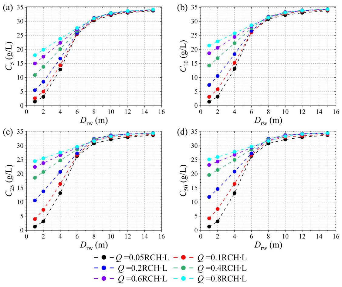
As shown in Figure A1, C increases monotonically with increasing, and for a given SA pattern, C also increases with t extending. This increase is particularly pronounced under conditions of higher Q (0.1 RCH∙L) and shallower (8 m), whereas only slight increases are observed for lower Q (0.1 RCH∙L) and/or deeper (8 m). Moreover, the rate of increase in C diminishes beyond approximately 25 years, and for most SA configurations, C approaches a quasi-steady state between 25 and 50 years. These results indicate that: (1) continuous SA leads to progressive increases in salt concentration at the extraction point, reflecting saltwater upconing processes; (2) the magnitude of salinity increase at the extraction point is strongly controlled by both Q and , with higher SA intensities and shallower depths producing more pronounced increases; and (3) over extended time scales, the aquifer system tends toward dynamic equilibrium, resulting in stabilization of extracted groundwater salt concentration.
References
- Kishi, Y.; Fukuo, Y. Studies on salinization of groundwater, I: Theoretical consideration on the three-dimensional movement of the salt water interface caused by the pumpage of confined groundwater in fan-shaped alluvium. J. Hydrol. 1977, 35, 1–29. [Google Scholar] [CrossRef] [Scilit]
- Agoubi, B. A review: Saltwater intrusion in North Africa’s coastal areas-current state and future challenges. Environ. Sci. Pollut. Res. 2021, 8, 17029–17043. [Google Scholar] [CrossRef] [Scilit]
- Jasechko, S.; Perrone, D.; Seybold, H.; Fan, Y.; Kirchner, J.W. Groundwater level observations in 250,000 coastal US wells reveal scope of potential seawater intrusion. Nat. Commun. 2020, 11, 3229. [Google Scholar] [CrossRef] [Scilit]
- Werner, A.D.; Sharp, H.K.; Galvis, S.C.; Post, V.E.; Sinclair, P. Hydrogeology and management of freshwater lenses on atoll islands: Review of current knowledge and research needs. J. Hydrol. 2017, 551, 819–844. [Google Scholar] [CrossRef] [Scilit]
- Fetter, C.W. Position of the saline water interface beneath oceanic islands. Water Resour. Res. 1972, 8, 1307–1315. [Google Scholar] [CrossRef] [Scilit]
- Van der Veer, P. Analytical solution for steady interface flow in a coastal aquifer involving a phreatic surface with precipitation. J. Hydrol. 1977, 34, 1–11. [Google Scholar] [CrossRef] [Scilit]
- Ghassemi, F.; Molson, J.W.; Falkland, A.; Alam, K. Three-dimensional simulation of the Home Island freshwater lens: Preliminary results. Environ. Model. Softw. 1998, 14, 181–190. [Google Scholar] [CrossRef] [Scilit]
- Sharan, A.; Lal, A.; Datta, B. A review of groundwater sustainability crisis in the Pacific Island countries: Challenges and solutions. J. Hydrol. 2021, 603, 127165. [Google Scholar] [CrossRef] [Scilit]
- Hussain, M.S.; Abd-Elhamid, H.F.; Javadi, A.A.; Sherif, M.M. Management of seawater intrusion in coastal aquifers: A review. Water 2019, 11, 2467. [Google Scholar] [CrossRef] [Scilit]
- Polemio, M.; Zuffianò, L.E. Review of utilization management of groundwater at risk of salinization. J. Water Resour. Plan. Manag. 2020, 146, 03120002. [Google Scholar] [CrossRef] [Scilit]
- Verruijt, A. An interface problem with a source and a sink in the heavy fluid. J. Hydrol. 1969, 8, 197–206. [Google Scholar] [CrossRef] [Scilit]
- Sherif, M.M.; Hamza, K.I. Mitigation of seawater intrusion by pumping brackish water. Transp. Porous Media 2001, 43, 29–44. [Google Scholar] [CrossRef] [Scilit]
- Kacimov, A.R.; Sherif, M.M.; Perret, J.S.; Al-Mushikhi, A. Control of sea-water intrusion by salt-water pumping: Coast of Oman. Hydrogeol. J. 2009, 17, 541–558. [Google Scholar] [CrossRef] [Scilit]
- Sowe, M.A.; Sadhasivam, S.; Mostafa Mohamed, M.; Mohsen, S. Modeling the mitigation of seawater intrusion by pumping of brackish water from the coastal aquifer of Wadi Ham, UAE. Sustain. Water Resour. Manag. 2019, 5, 1435–1451. [Google Scholar] [CrossRef] [Scilit]
- Abd-Elaty, I.; Javadi, A.A.; Abd-Elhamid, H. Management of saltwater intrusion in coastal aquifers using different wells systems: A case study of the Nile Delta aquifer in Egypt. Hydrogeol. J. 2021, 29, 1767–1783. [Google Scholar] [CrossRef] [Scilit]
- Mahesha, A. Control of seawater intrusion through injection-extraction well system. J. Irrig. Drain. Eng. 1996, 122, 314–317. [Google Scholar] [CrossRef] [Scilit]
- Ebeling, P.; Händel, F.; Walther, M. Potential of mixed hydraulic barriers to remediate seawater intrusion. Sci. Total Environ. 2019, 693, 133478. [Google Scholar] [CrossRef] [Scilit]
- Park, S.U.; Kim, J.M.; Yum, B.W.; Yeh, G.T. Three-dimensional numerical simulation of saltwater extraction schemes to mitigate seawater intrusion due to groundwater pumping in a coastal aquifer system. J. Hydrol. Eng. 2012, 17, 10–22. [Google Scholar] [CrossRef] [Scilit]
- Rastogi, A.K.; Choi, G.W.; Ukarande, S.K. Diffused interface model to prevent ingress of sea water in multi-layer coastal aquifers. J. Spat. Hydrol. 2004, 4, 2. [Google Scholar]
- Yu, W.; Baù, D.; Mayer, A.S.; Mancewicz, L.; Geranmehr, M. Investigating the impact of seawater intrusion on the operation cost of groundwater supply in island aquifers. Water Resour. Res. 2023, 59, e2023WR034798. [Google Scholar] [CrossRef] [Scilit]
- Ho, H.C.; Mylroie, J.E.; Infante, L.R.; Rodgers, J.C. Fuzzy-based spatial modelling approach to predict island karst distribution: A conceptual model. Environ. Earth Sci. 2014, 71, 1369–1377. [Google Scholar] [CrossRef] [Scilit]
- McGee, D.K.; Wynn, J.G.; Onac, B.P.; Harries, P.J.; Rothfus, E.A. Tracing groundwater geochemistry using δ13C on San Salvador Island (southeastern Bahamas): Implications for carbonate island hydrogeology and dissolution. Carbonates Evaporites 2010, 25, 91–105. [Google Scholar] [CrossRef] [Scilit]
- Martin, J.B.; Moore, P.J. Sr concentrations and isotope ratios as tracers of ground-water circulation in carbonate platforms: Examples from San Salvador Island and Long Island, Bahamas. Chem. Geol. 2008, 249, 52–65. [Google Scholar] [CrossRef] [Scilit]
- Davis, R.L.; Johnson, C.R. Karst hydrology of San Salvador. In Proceedings of the Fourth Symposium on the Geology of the Bahamas; Mylroie, J.E., Ed.; Bahamian Field Station: San Salvador Island, Bahamas, 1989; pp. 118–135. [Google Scholar]
- Moore, P.J. Controls on the Generation of Secondary Porosity in Eogenetic Karst: Examples from San Salvador Island, Bahamas and North-Central Florida, USA. Ph.D. Thesis, University of Florida, Gainesville, FL, USA, 2009. [Google Scholar]
- Langevin, C.D.; Thorne, D.T., Jr.; Dausman, A.M.; Sukop, M.C.; Guo, W. SEAWAT Version 4: A Computer Program for Simulation of Multi-Species Solute and Heat Transport. In U.S. Geological Survey Techniques and Methods; U.S. Geological Survey: Reston, VA, USA, 2008; Volume Book 6, Chapter A22; pp. 1–39. [Google Scholar] [CrossRef] [Scilit]
- Gulley, J.D.; Mayer, A.S.; Martin, J.B.; Bedekar, V. Sea level rise and inundation of island interiors: Assessing impacts of lake formation and evaporation on water resources in arid climates. Geophys. Res. Lett. 2016, 43, 9712–9719. [Google Scholar] [CrossRef] [Scilit]
- Holding, S.; Allen, D.M. From days to decades: Numerical modelling of freshwater lens response to climate change stressors on small low-lying islands. Hydrol. Earth Syst. Sci. 2015, 19, 933–949. [Google Scholar] [CrossRef] [Scilit]
- Yu, W.; Baù, D.; Mayer, A.S.; Geranmehr, M. An efficient surrogate-based multi-objective optimisation framework with novel sampling strategy for sustainable island groundwater management. Adv. Geosci. 2024, 64, 23–26. [Google Scholar] [CrossRef] [Scilit]
- Yu, W.; Zhang, Y. Impacts of sea-level rise and recharge fluctuations on cutoff wall effectiveness for freshwater lens development and seawater intrusion mitigation in unconfined island aquifers. Hydrology 2026, 13, 76. [Google Scholar] [CrossRef] [Scilit]
- Volker, R.E.; Mariño, M.A.; Rolston, D.E. Transition zone width in ground water on ocean atolls. J. Hydraul. Eng. 1985, 111, 659–676. [Google Scholar] [CrossRef] [Scilit]
- Budd, D.A.; Vacher, H.L. Predicting the thickness of fresh-water lenses in carbonate paleo-islands. J. Sediment. Res. 1991, 61, 43–53. [Google Scholar] [CrossRef] [Scilit]
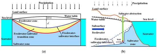
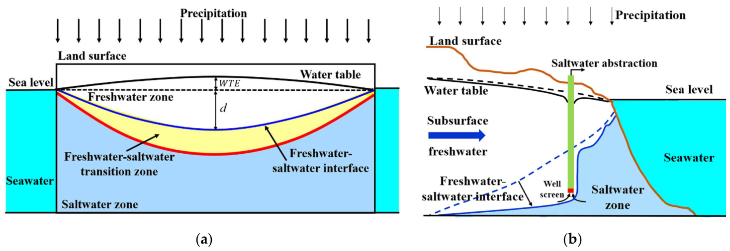
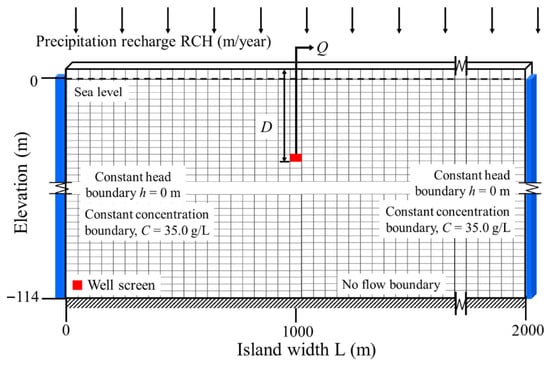
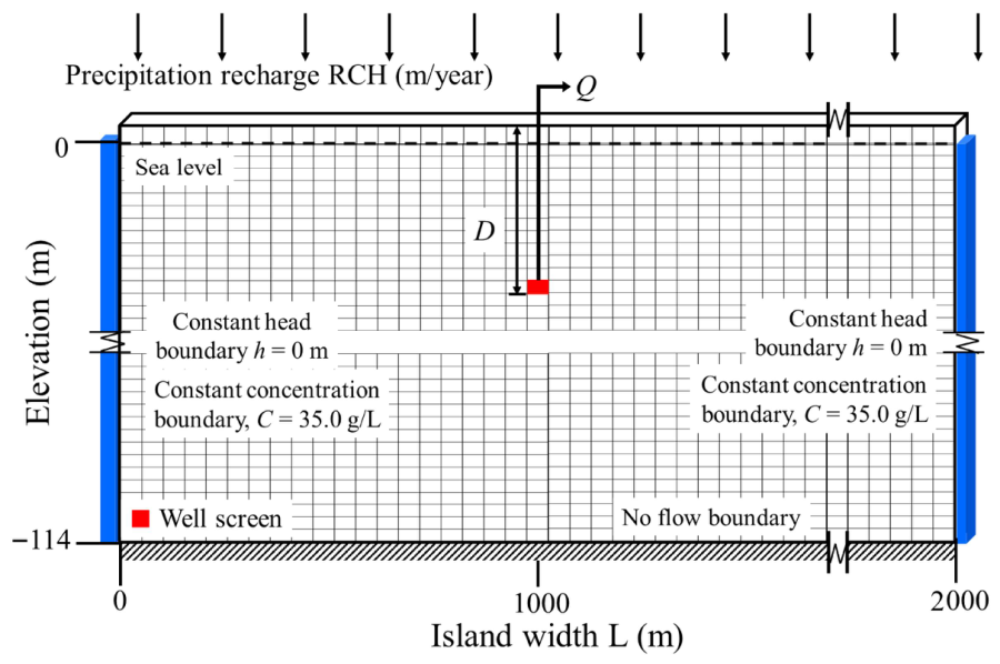
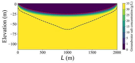
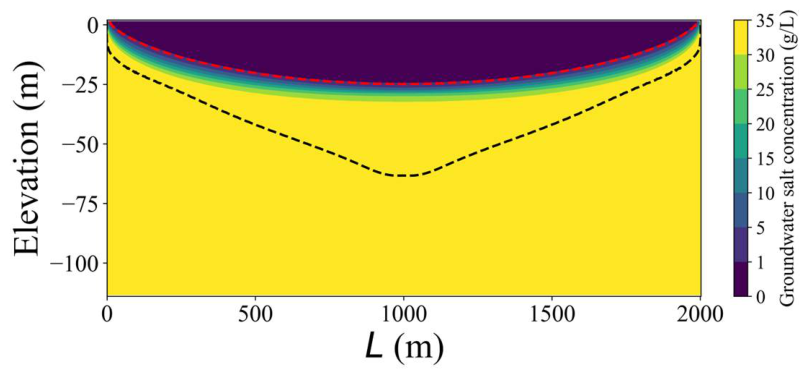
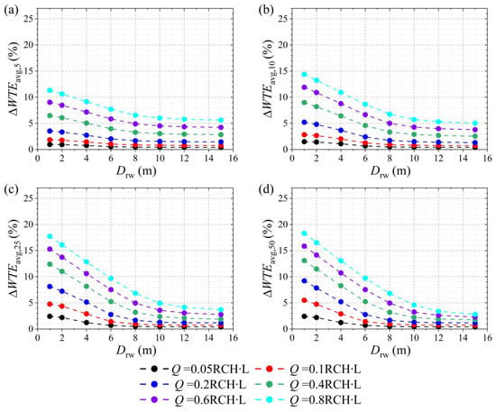
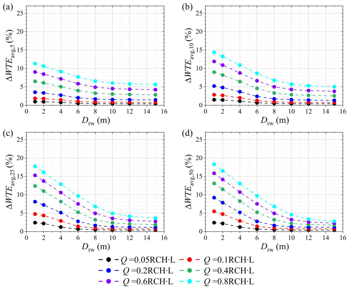
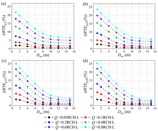
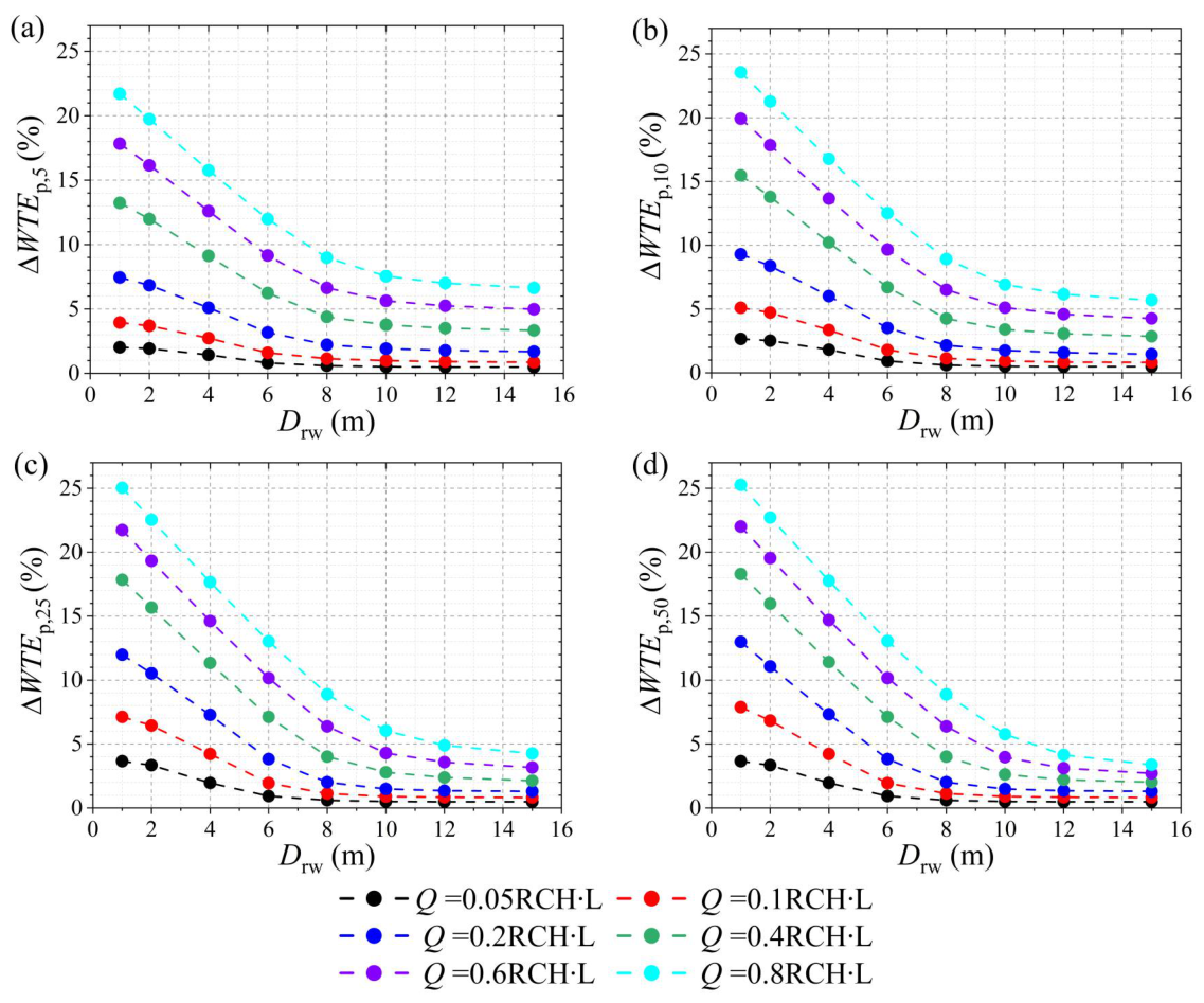
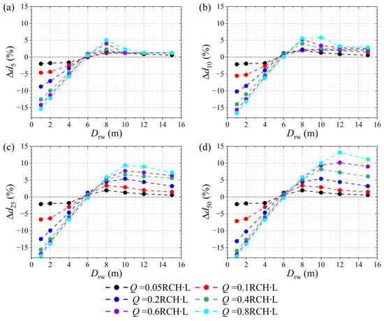
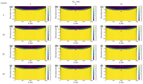
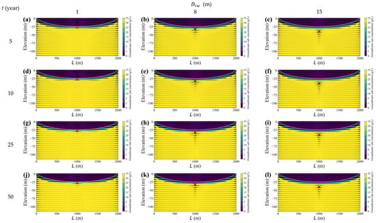
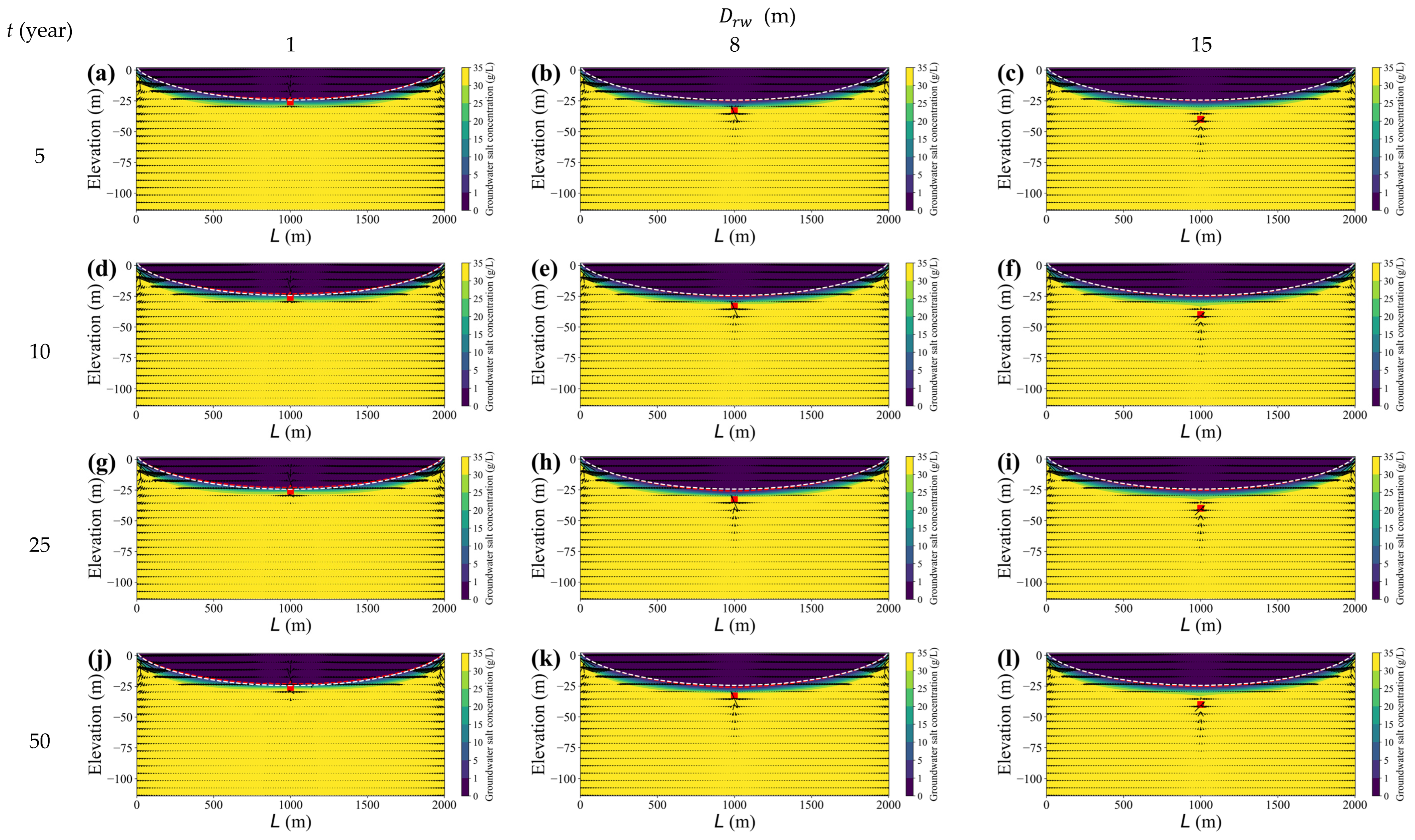
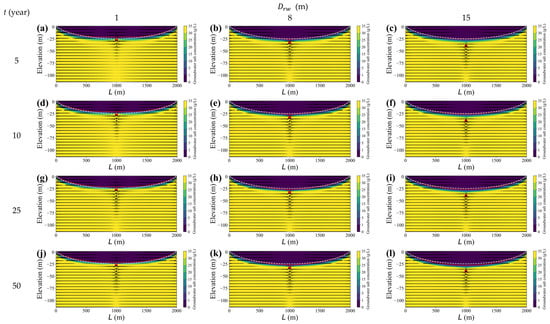
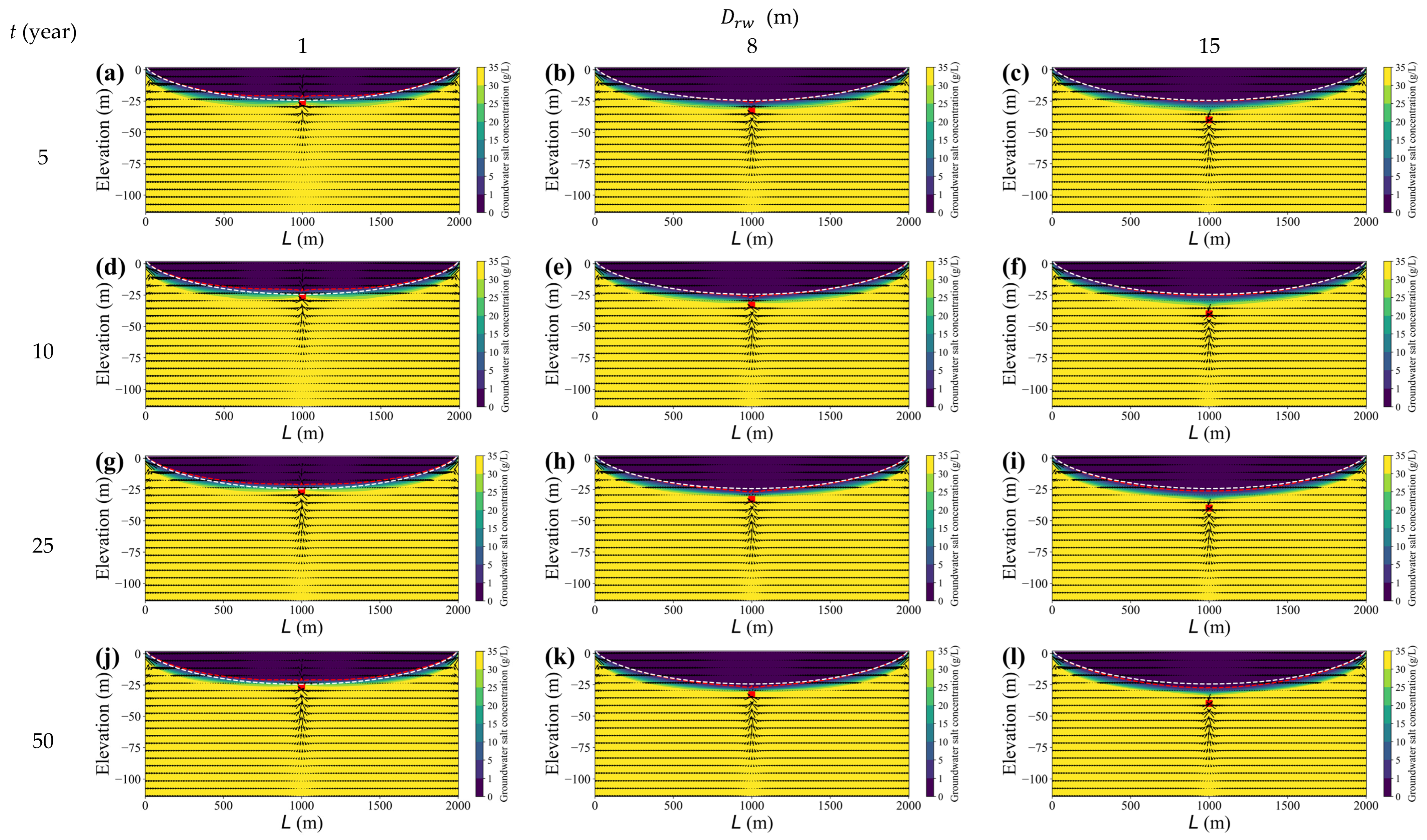
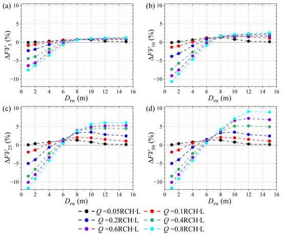
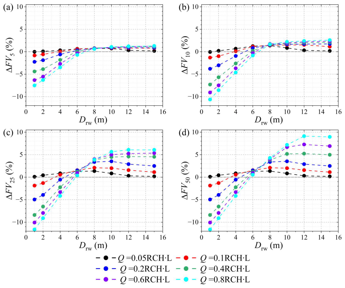
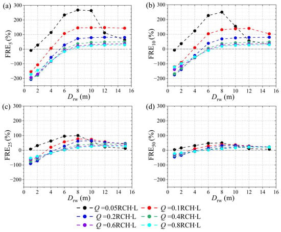
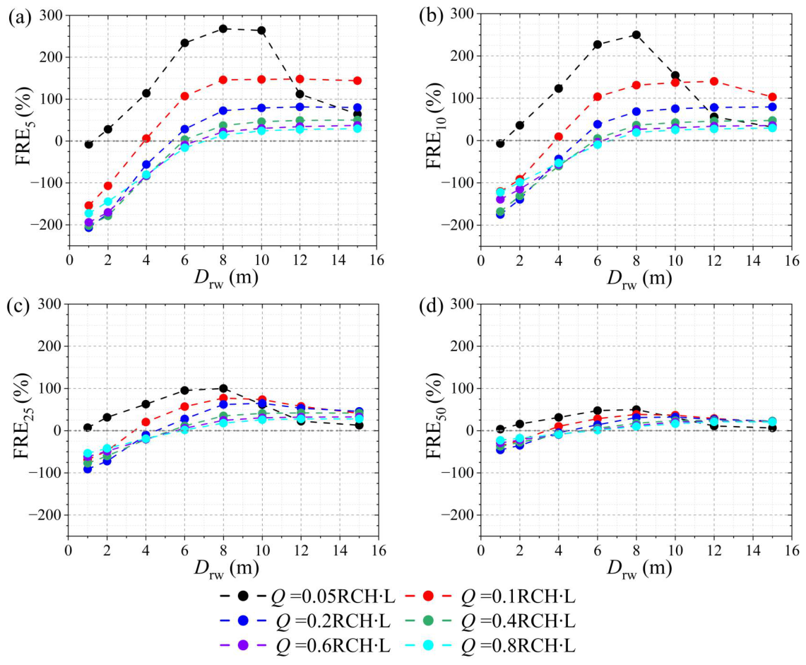
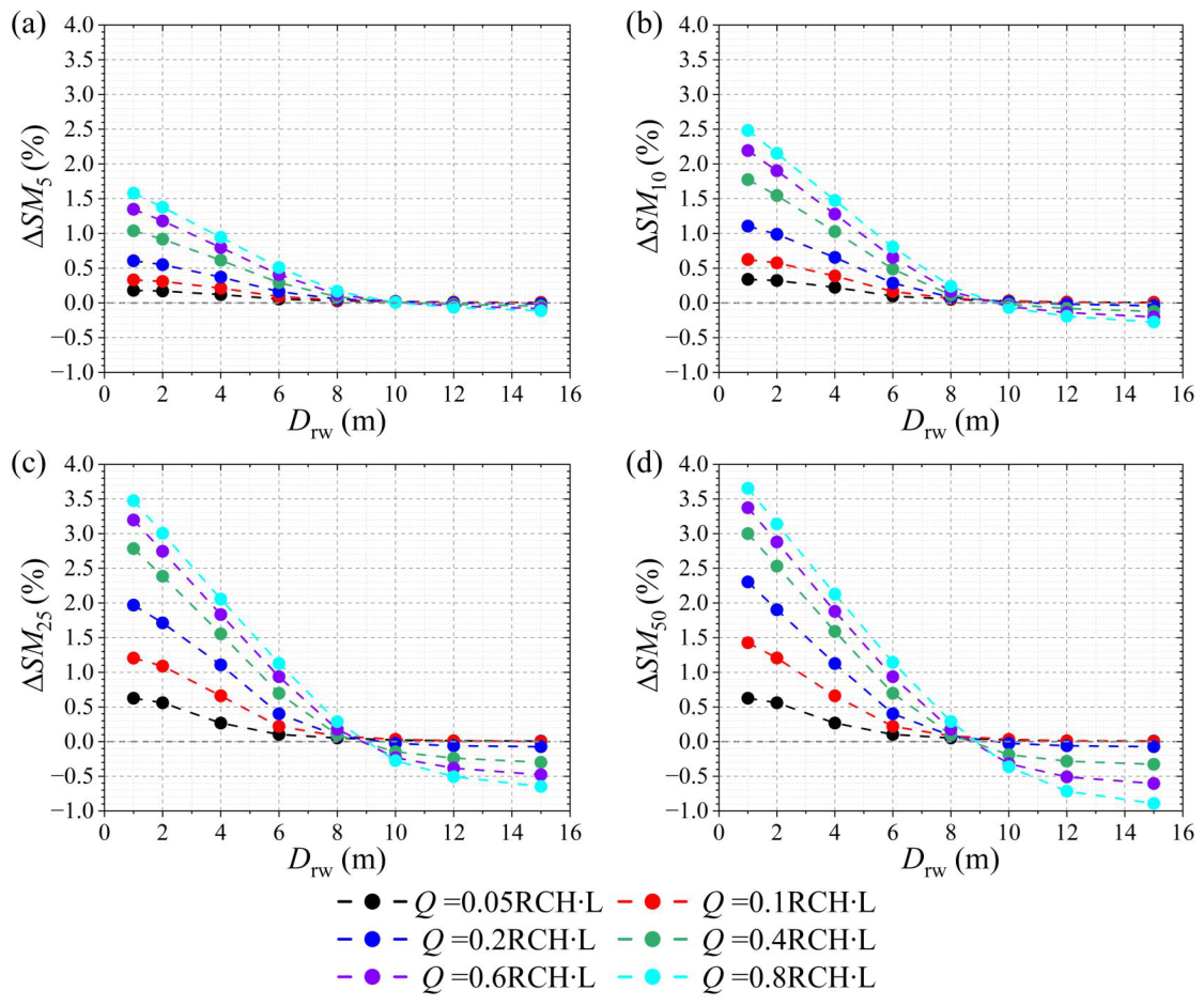

Disclaimer/Publisher’s Note: The statements, opinions and data contained in all publications are solely those of the individual author(s) and contributor(s) and not of MDPI and/or the editor(s). MDPI and/or the editor(s) disclaim responsibility for any injury to people or property resulting from any ideas, methods, instructions or products referred to in the content. |
© 2026 by the authors. Licensee MDPI, Basel, Switzerland. This article is an open access article distributed under the terms and conditions of the Creative Commons Attribution (CC BY) license.