Numerical Simulation of Rainfall-Induced Debris Flows Triggered by Cyclone Yaku 2023 in Chasquitambo, Peru

Abstract

Debris flows are rapid downslope movements of soil and rock (a type of external geodynamic process) typically triggered by extreme rainfall, posing significant threats to infrastructure and human lives. The objective of this study is to assess the relationship between rainfall intensity and debris flow magnitude for different return periods (5, 10, 50, and 100 years) and, ultimately, to establish rainfall thresholds in Chasquitambo (Perú). This work presents numerical simulation results for extreme rainfall scenarios using the open-source software HEC-RAS v6.4.1 (Mud/Debris Flow mode), calibrated with flood marks from the recent extreme Cyclone Yaku event that occurred on 12 March 2023 (considered an approximately 100-year event). The simulations reveal a non-linear relationship between rainfall intensity and hazard, with the most extensive impacts reaching velocities of 4.5 m/s, depths of up to 7.0 m, and affecting an area of ~130,000 m². The study indicates an operational rainfall threshold of 20 mm in 24 h, which is proposed to trigger monitoring protocols, early warning systems, and effective mitigation strategies. The proposed workflow provides a transferable and data-efficient foundation for deriving operational rainfall thresholds and scenario-based hazard metrics, which are useful for early warning systems and land-use planning in similar mountain catchments.

1. Introduction

There is a pressing need to understand the dynamics of debris flows triggered by extreme rainfall events. Achieving a quantitative and precise understanding of these processes is crucial for engaging stakeholders in risk governance through the implementation of structural and non-structural mitigation measures grounded in scientific evidence.

Globally, debris flows account for approximately 90% of rainfall-related disasters in mountain areas. Their frequency and magnitude have increased due to land-use change and climate change [1], causing widespread infrastructure damage and loss of life [2]. In Peru, between 2003 and 2020, around 2276 debris flow events were recorded, of which 169 occurred in the Ancash region [3]. One of these events took place in Chasquitambo on 12 March 2023 as a result of Cyclone Yaku [4], producing damages that overwhelmed the response capacity of local governments.

Robust debris flow hazard assessment typically requires long-term rainfall records (≥30 years), high-resolution topography, and well-documented events for model calibration. In most Andean catchments, these critical inputs are severely limited or entirely unavailable; extreme rainfall events with long return periods are the main triggers of debris flows [5]. The propagation of a debris flow is further influenced by local topography, the rheological properties of the material, antecedent hydrological conditions, and vegetation cover [6]. In addition, climate change, population growth, and deforestation contribute to increasing the debris flow hazard and risk [1].

The use of computational models is essential for simulating debris flow processes [7]. These models can reproduce the transport and deposition dynamics of the flow. Some models are based on smoothed particle hydrodynamics or semi-implicit particle methods [8], allowing spatial and temporal predictions that consider topography, material characteristics, and hydrological conditions [9], calibrated with field and laboratory parameters [10]. Finite difference methods are frequently employed in debris flow modeling, based on the principles of continuum mechanics (conservation of mass, energy, and momentum) to capture dynamic flow motion while incorporating appropriate rheological models [11]. Various physical models have been developed to simulate debris flows, with specific utilities for granular-avalanche flows [12], large landslides [13], and hyperconcentrated flows [14]. While some offer advantages in coupled rainfall–runoff simulations, none capture all processes comprehensively; however, recent advances in two-phase models have improved realism [15].

In addition to physics-based modeling, the debris flow literature has extensively developed rainfall thresholds for early warning activation, either through empirical intensity–duration approaches or using accumulated variables and antecedent conditions [16]. The classic global threshold proposed by Caine [17] and its subsequent updates show that as rainfall duration increases, the minimum mean intensity capable of triggering shallow landslides and debris flows decreases, which supports the use of I-D curves when sub-hourly data are available. In contexts with limited records and absence of sub-daily rainfall data, several authors recommend using operational thresholds based on daily accumulations, explicitly acknowledging their uncertainty and updating them in light of recent extreme events [18,19]. More recently, methodologies have been proposed that link the threshold not only to initiation but also to hazardous magnitude, which is particularly relevant in basins with few documented events [20].

In Peru, despite the high incidence of huaicos (debris flows), published numerical simulation studies are scarce; for instance, Díaz-Salas [5] modeled a dam break-triggered flow in Ancash; Asencios [21] reported a case in Chosica, Lima; and the IGP [7] simulated a flow in the Záparo ravine; nevertheless, these studies share limitations in calibration because they are conducted using moderate-magnitude events (typically with a return period of less than 10 years), and the topographic resolution (≥1 m) is insufficient to capture the interaction of flow with infrastructure in urban areas [22,23].

Some studies in the Colombian Andes [24] and Peru [22,23] have begun to address data scarcity through UAV-based topography and multi-model comparisons. Cardona et al. [24] modeled debris flows under data-scarce conditions using DEMs of ≥12.5 m, acknowledging that the lack of high-resolution topography and the absence of calibration with documented extreme events limit the transferability of model parameters to hazard scenarios beyond the calibration range. Similarly, Chacon et al. [23] applied HEC-RAS 2D in Apurímac, Peru, calibrating with one event for a 5-year return period. None of these studies employed an ultra-high-resolution DEM, calibrated with a documented extreme event, or explored scenarios with multiple return periods to quantify the non-linear scaling of hazards.

In summary, this study contributes a back-analysis of the debris flow event associated with Cyclone Yaku 2023 using field markers and a 0.12 m drone-derived DEM; a calibrated 2D simulation framework in HEC-RAS (Mud/Debris Flow mode) [25] for four design storms (RP 5–100 years); quantitative hazard metrics (depth, velocity, affected area) that demonstrate non-linear scaling with rainfall severity; and an operational 24 h rainfall threshold for monitoring activation, early warning, and risk governance in an Andean context with limited data.

The primary objective is to assess the relationship between rainfall intensity and debris flow magnitude for different return periods (5, 10, 50, and 100 years) and, ultimately, to establish rainfall thresholds for Chasquitambo (Peru), providing essential data for activating monitoring protocols, early warning systems, and land-use planning and disaster risk management strategies in the study area.

2. Materials and Methods

2.1. Study Area

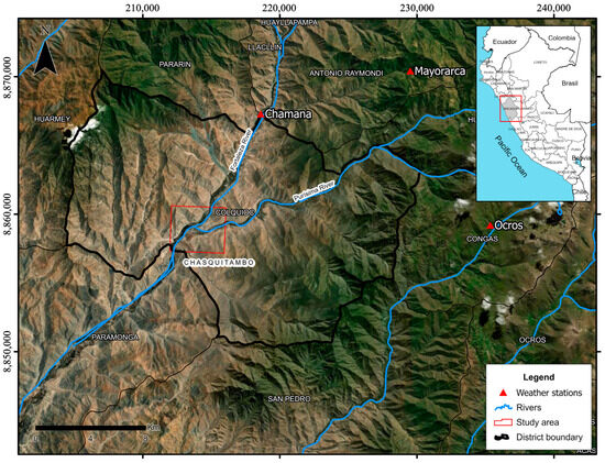
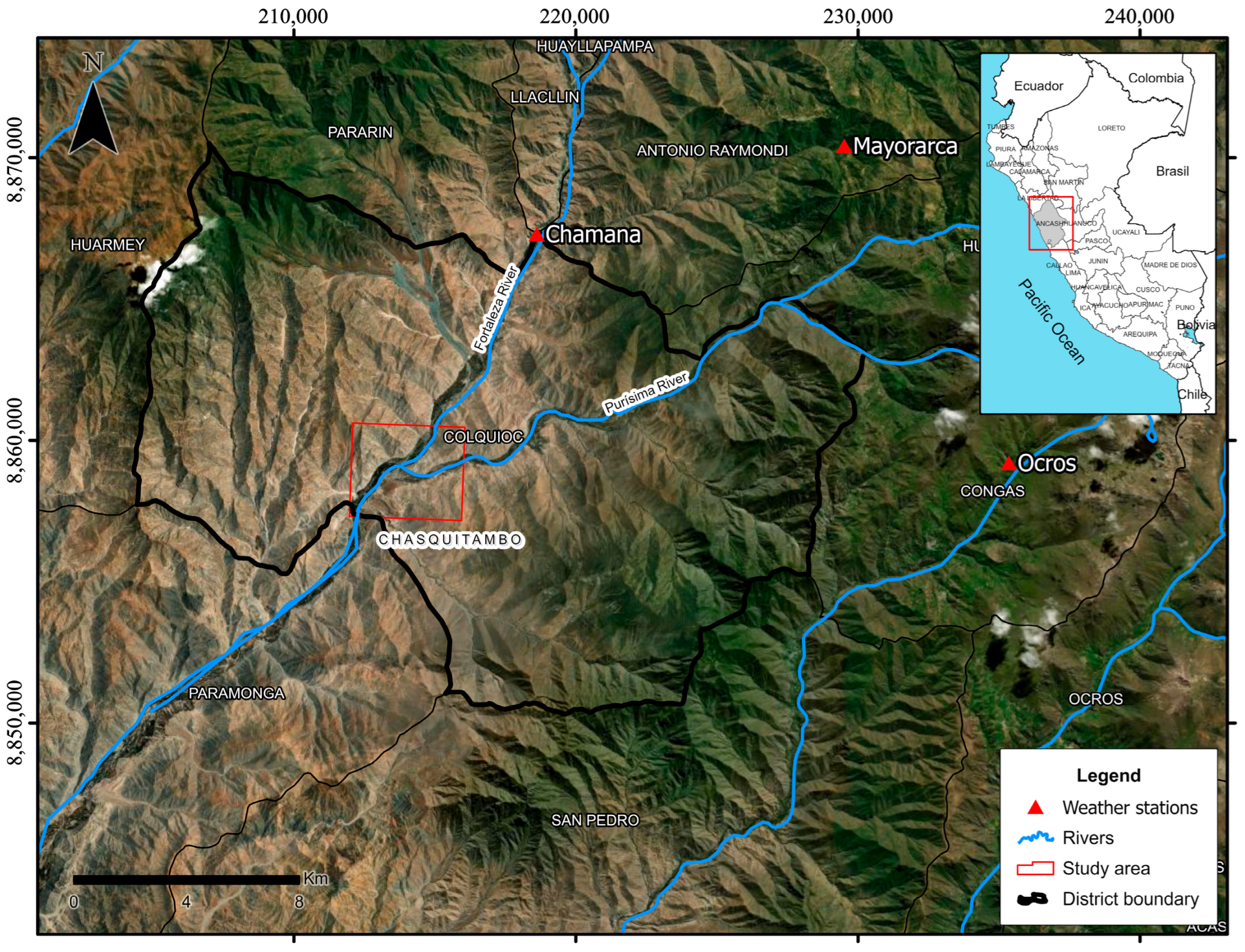
Chasquitambo is located on the Peruvian coast within Colquioc District, Bolognesi Province, Ancash Department. It lies on the left bank of the Purísima River at its confluence with the Fortaleza River (Figure 1). The local geomorphology is characterized by an alluvial fan composed of gravelly sediment deposits over a structural mountainous basement of intrusive rock. The region experiences an arid climate with mild temperatures and a year-round moisture deficit.

Figure 1. Location of the study area (Chasquitambo, Ancash region, Peru).

The El Niño phenomenon develops in the tropical Pacific Ocean, particularly in region 1 + 2, which is an area close to the coasts of Ecuador and Peru, with direct impacts on the Peruvian coast [26]. It induces changes in ocean–atmosphere coupling in the equatorial Pacific [27], including increased thermal stratification [28] and heightened rainfall over the continent [29]. This phenomenon involves several associated disturbances such as the Madden–Julian Oscillation (MJO), the arrival of westerly wind bursts, and warm Kelvin waves [30]. In March 2023, during a period of elevated sea surface temperatures in the Pacific and an anomalous phase of the MJO [31], a non-organized, low-pressure, tropical-like cyclonic system known as Yaku developed [32]. This system contributed to a positive feedback loop that reinforced warm oceanic conditions and triggered intense precipitation across the northern–central coastal and Andean regions of Peru [27], surpassing historical rainfall records. These anomalous conditions led to the activation of normally dry ravines and widespread flooding, with daily rainfall anomalies exceeding 25 mm/day during March 2023 [32]. Approximately 522,200 people were affected, and nearly 30,000 dwellings were rendered uninhabitable, with the departments of Tumbes, Piura, Lambayeque, La Libertad, Ancash, Lima, and Ica suffering the most severe losses [4].

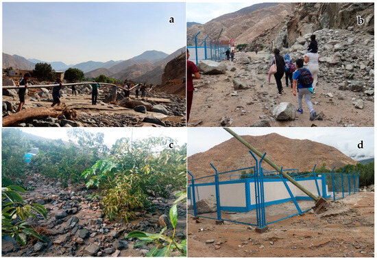
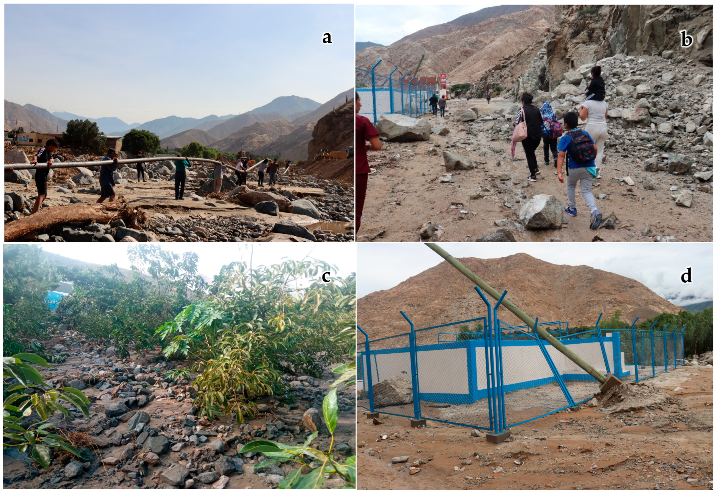
On 12 March 2023, extreme rainfall associated with Cyclone Yaku caused the Purísima River to convey intense debris flows, which eventually overtopped its banks, resulting in significant damage. Approximately 81 homes and one educational institution were impacted; 3500 m of rural roads were affected; 14,825 m of irrigation infrastructure were destroyed; 130 m of sewer network were damaged; and 5.11 hectares of permanent crops were lost [4]. Figure 2 illustrates the spatial extent of the debris flow inundation in the urban area of Chasquitambo, showing deposits of gravel and cobbles up to 0.8 m thick. The distribution and thickness of these coarse sediments confirm the high-energy nature of the event and corroborate the selection of representative cross-sections downstream for model calibration. By its magnitude (exceeding all previously recorded values in the area), this event is considered equivalent to roughly a 100-year return period.

Figure 2. Evidence of debris flow impacts from the 12 March 2023 event in Chasquitambo: (a) Damage to a potable water pipeline; (b) debris deposition on a roadway; (c) destruction of permanent crops; (d) damage to public infrastructure.

Climate projections indicate that by the end of the 21st century, this region will experience increases in the intensity of extreme precipitation events. Additionally, the frequency of such events may rise by 20–30% between 2050 and 2100, particularly during the months of December to March [33].

2.2. Drone-Based Photogrammetry

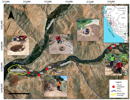
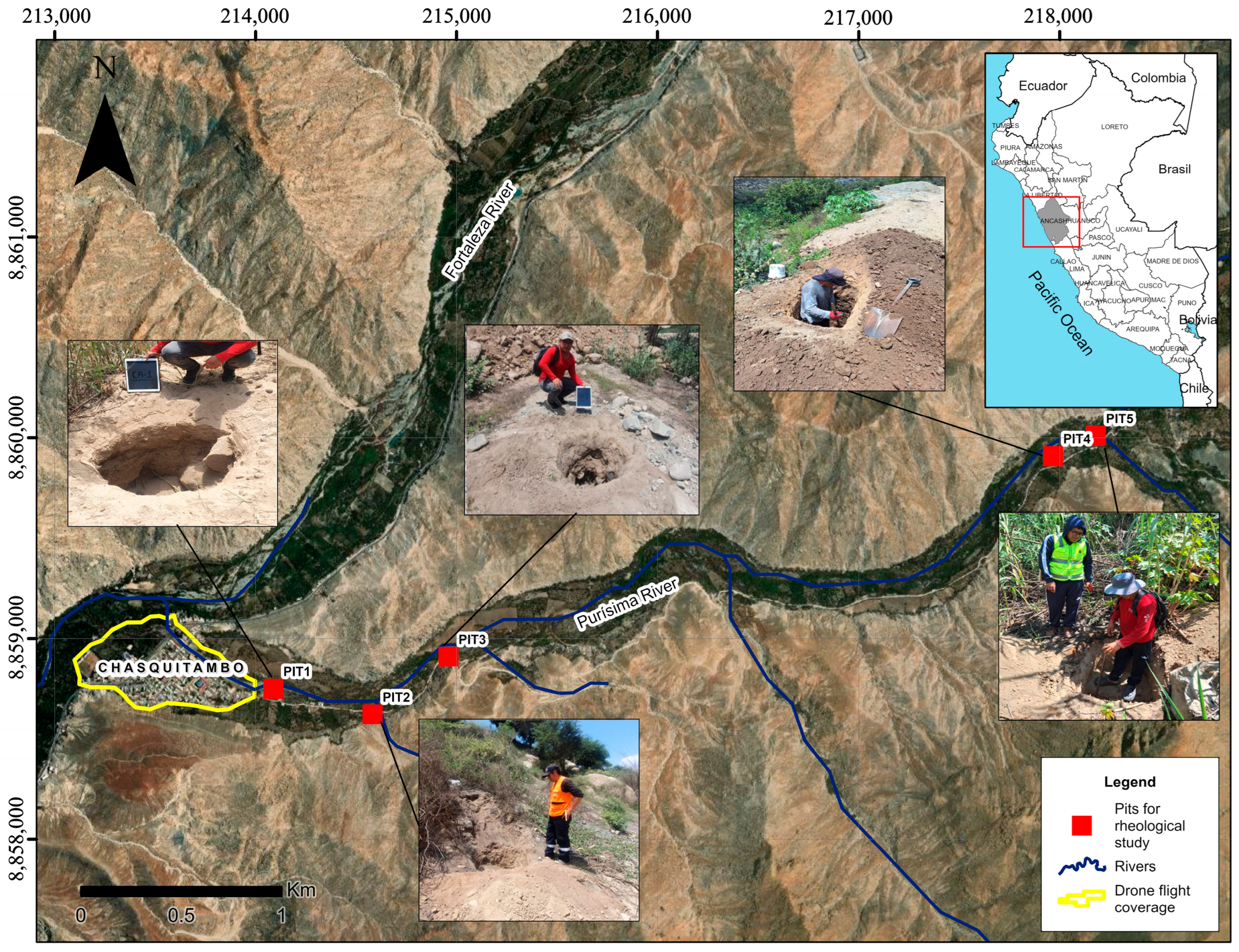
Photogrammetry was used to obtain a high-resolution topographic base for modeling. Flight planning was conducted to define key parameters such as target resolution and the coverage area (Figure 3). A DJI Phantom 4 Pro v2 drone was utilized, with the flight plan configured to capture vertical images with 70% overlap to ensure full coverage. Fifteen ground control points were established using a differential GPS (accuracy ±0.03 m) for georeferencing, with the flight taking place in February 2024. Image processing was carried out using MeshLab software version 2023.12, involving image orientation, generation of a dense point cloud, and creation of a Digital Elevation Model (DEM) with 0.12 m spatial resolution, along with an orthophoto of the area.

Figure 3. Location of test pits and photogrammetry survey area.

2.3. Rainfall–Runoff Modeling

Since hourly rainfall records were not available for the area, the analysis was conducted using daily maximum rainfall data (24 h totals) from 1981 to 2023, obtained from the National Meteorology and Hydrology Service of Peru (SENAMHI). Data from the Chamana, Mayorarca, and Ocros meteorological stations were selected for their spatial coverage and period of record. As detailed in Table 1, these stations exhibit a pronounced gradient in annual maximum daily rainfall (AMDR) characteristics—from the highly variable coastal regime at Chamana (max: 70.0 mm, σ: 16.21 mm) to the more moderate highland regimes at Mayorarca and Ocros. This variability directly informs the intensity–duration–frequency analysis and provides the rainfall forcing scenarios essential for realistic debris flow modeling in the Chasquitambo basin. Missing data were infilled and extended via linear regression using neighboring station records. Based on the Kolmogorov–Smirnov goodness-of-fit test, a Log-Normal distribution was adopted for the Chamana and Ocros stations, while a Log-Pearson Type III distribution was chosen for Mayorarca. The best-fit statistical distributions were identified, and intensity–duration–frequency (IDF) curves were generated for each site. Design storm hyetographs were then constructed using the alternate block method of Dyck–Peschke. This method distributes rainfall by placing the maximum intensities at the mid-duration, generating a centered-peak storm [34].

Table 1. Characteristics of the meteorological stations and descriptive statistics of the annual maximum daily rainfall (AMDR) used in the frequency analysis (period 1981–2023).

Name	Coordinates	Altitude (masl)	Distance to Chasquitambo	Record Period	AMDR—Min (mm)	AMDR—Max (mm)	AMDR—Mean (mm)	AMDR—Std. Dev. (mm)
Chamana	Lat: 10°12′26.6″ Long: 77°33′31.41″	1228	9.5 km	1981–2023 (43 years)	2.80	70.00	15.90	16.21
Mayorarca	Lat: 10°9′27.91″ Long: 77°20′56.01″	3335	19.43 km	1981–2023 (43 years)	10.40	50.20	21.50	7.51
Ocros	Lat: 10°24′16.46″ Long: 77°24′0.90″	3249	21.58 km	1981–2023 (43 years)	10.50	38.00	19.70	6.19

Subsequently, rainfall–runoff modeling was performed using the Curve Number (CN) method implemented in HEC-HMS software version 4.11. The model inputs included the morphometric characteristics of the Purísima watershed (also referred to as the Purísima hydrographic unit). Unit hydrographs (design flood hydrographs) were generated for return periods of 5, 10, 50, and 100 years.

2.4. Rheology

Key rheological parameters (yield stress and dynamic viscosity of the debris flow mixture) were estimated using empirical formulas proposed by O’Brien and Julien. In particular, two equations (Equation (1) for dynamic viscosity and Equation (2) for yield stress) [35] were applied, using results from laboratory sediment analyses. These equations relate the rheology to sediment concentration and grain size characteristics.

$$n={\alpha }_1{e}^{{\beta }_1{C}_v}$$

(1)

$${\tau }_y={\alpha }_2{e}^{{\beta }_2{C}_v}$$

(2)

where n is the dynamic viscosity of the mixture, ${\tau }_y$ is the yield stress, ${\alpha }_i$ and ${\beta }_i$ are empirical coefficients dependent on sediment size distribution, and $C_v$ is the volumetric sediment concentration.

Table 2 summarizes the results of the granulometric analysis of five soil samples from the study area. Sediment grain-size distributions and Atterberg limits were obtained for each sample. The samples were collected from test pits of dimensions 1.5 m (depth) × 1 m × 1 m. Three samples (CA-01, CA-02, CA-05) were taken from the channels of the main ravines contributing debris to the Purísima River, and two samples (CA-03, CA-04) were taken from areas adjacent to the river, as shown in Figure 3, and are representative of deposits from the study event. Grain-size analysis and Unified Soil Classification System (USCS) classifications were provided by an INDECOPI-accredited laboratory (Table 2).

Table 2. Results of granulometric analysis. USCS—Unified Soil Classification System; D16, D50, and D84 are grain diameters corresponding to 16%, 50%, and 84% finer by weight.

Test Pit	USCS Classification	Gravel (%)	Sand (%)	Fines (%)	D16 (mm)	D50 (mm)	D84 (mm)	Liquid Limit (%)	Plastic Limit (%)
CA-01	SM (silty sand)	15.23	62.17	22.60	0.03	1.05	4.62	19.65	16.34
CA-02	SM (silty sand with gravel)	23.41	54.87	21.72	0.03	0.87	20.99	-	-
CA-03	SW SM (well-graded sand with silt and gravel)	46.35	46.89	6.75	0.64	4.10	29.67	-	-
CA-04	GW GC (well-graded gravel with clay and silt)	47.19	47.00	5.81	0.71	4.28	30.88	-	-
CA-05	SM (silty sand with gravel)	16.23	60.28	23.49	0.02	1.05	4.91	23.47	20.03

According to the USCS classification, CA-01 is silty sand (SM); CA-02 is silty sand with gravel (SM); CA-03 is well-graded sand with silt and gravel (SW-SM); CA-04 is well-graded gravel with clay and silt (GW-GC); and CA-05 is silty sand with gravel (SM).

To select appropriate rheological parameters for the simulations, the grain-size results were compared with reference data from O’Brien and Julien [35]. Table 3 presents characteristics of several reference debris flow mixtures (mudflow matrix properties) from O’Brien and Julien, alongside the local sample data. The soils in Chasquitambo have an average fine fraction (16% silt + clay) and low plasticity, comparable to the “Glenwood Sample 2” reference, which also has low clay content and predominantly sandy-gravel composition. Thus, the Glenwood sample 2 rheological coefficients were adopted for the model.

Table 3. Properties of mudflow matrix (fine fraction) from O’Brien and Julien reference datasets, compared to local conditions.

Sample	Sediment Size Distribution				Liquid Limit (%)	Plastic Limit (%)
	Clay (%)	D16 (mm)	D50 (mm)	D84 (mm)
Glenwood original	4.8	0.01	0.034	0.062	-	-
Glenwood sample 1	6.8	0.009	0.023	0.050	-	-
Glenwood sample 2	3.0	0.016	0.035	0.061	-	-
Glenwood sample 3	4.8	0.011	0.025	0.053	-	-
Glenwood sample 4	7.6	0.001	0.018	0.032	-	-
Aspen pit 1	31.3	0.001	0.011	0.032	32	11
Aspen natural soil	27.0	0.001	0.012	0.028	25	06
Aspen mine fill	27.8	0.001	0.013	0.030	24	06
Aspen natural soil source	31.6	0.001	0.016	0.039	-	-
Aspen mine fill source	25.2	0.001	0.018	0.061	-	-
Chasquitambo (avg.)	16	see Table 2	see Table 2	see Table 2	22	18

The rheological characterization of the debris flow mixture from Chasquitambo was performed by adapting the empirical coefficients (α and β) derived from Glenwood sample 2. Using Equations (1) and (2), which relate sediment concentration and fine-fraction properties to yield stress and viscosity, the rheological parameters adopted in the simulation were obtained and are summarized in Table 4.

Table 4. Rheological coefficients adopted for the debris flow model.

Source (Sample)	$\mathbf{Yield} \mathbf{Stress}, {\mathit{\tau }}_{\mathit{y}}$ (Pa)	$\mathbf{Dynamic} \mathbf{Viscosity}, \mathit{n}$ (Pa-s)
Glenwood sample 2	10.704	0.0762

2.5. Debris Flow Modeling

The debris flow simulation was conducted with a two-dimensional (2D) hydraulic model using HEC-RAS (v6.4.1, Mud/Debris Flow mode). This software was selected despite its recognized limitations in adequately simulating erosive processes, the abrupt deposition of highly viscous flows, and the dynamic formation of large debris dams; the choice was justified by its open-access nature and widespread use, which enhances the transferability and utility of the methodology for other contexts. Furthermore, its input parameter requirements are comparatively more attainable than those of specialized alternatives—a decisive factor for regions with limited instrumentation, such as Peru.

The modeling process began by constructing a high-resolution terrain model from the drone-derived DEM. The domain was discretized with a computational mesh using square grid cells of 2 m, with finer resolution (0.5 m cell size) along the river channel centerline to better capture flow dynamics. Key topographic features, such as channel banks, were represented using breaklines in the mesh. Inflow and outflow boundary conditions were defined based on the watershed delineation and topography (inflow hydrograph from the upstream catchment and free outflow at the downstream end of the study reach). The time step configured for the simulation was 1 s. Manning’s n roughness coefficients were assigned based on field observations: 0.037 for the river channel, 0.050 for channel banks/margins, 0.045 for the urbanized area, and 0.035 for agricultural fields. It is recognized that roughness in debris flows can vary dynamically due to changes in sediment concentration, erosion, and deposition. Although the current model does not incorporate this dynamic behavior, the sensitivity analysis demonstrates the impact of this uncertainty on the results.

The HEC-RAS solver employs a finite-difference scheme to compute debris flow propagation, solving the depth-averaged shallow water equations (Saint-Venant equations) adapted for debris flow. The governing equations include the continuity equation (Equation (3)) and momentum conservation equations in the x and y directions (Equations (4) and (5)) [25]. These equations account for gravitational acceleration, pressure forces, and frictional resistance and were augmented to include additional terms for sediment concentration and non-Newtonian flow behavior as per the chosen rheological model.

$${\displaystyle \frac{\partial h}{\partial t}}+{\displaystyle \frac{\partial h{V}_x}{\partial x}}+{\displaystyle \frac{\partial h{V}_y}{\partial y}}=i$$

(3)

$$S_{fx}=S_{ox}-{\displaystyle \frac{\partial h}{\partial x}}-{\displaystyle \frac{V_x\partial V_x}{g\partial x}}-{\displaystyle \frac{V_y\partial V_y}{g\partial y}}-{\displaystyle \frac{1\partial V_x}{g\partial t}}$$

(4)

$$S_{fy}=S_{oy}-{\displaystyle \frac{\partial h}{\partial y}}-{\displaystyle \frac{V_y\partial V_y}{g\partial y}}-{\displaystyle \frac{V_x\partial V_y}{g\partial x}}-{\displaystyle \frac{1\partial V_y}{g\partial t}}$$

(5)

where $h$ is the flow depth; $V_x$ and $V_y$ are the depth-averaged velocity components along the X and Y axes, respectively; $S_{fx}$ and $S_{fy}$ are the friction slope components; and $S_{ox}$ and $S_{oy}$ are the bed slopes in the respective directions.

Yield stress effects were incorporated via an equilibrium stress approach. The yield stress of the debris flow mixture was computed using Equation (6) [36], assuming steady fully developed flow conditions for the mixture’s internal stress.

$$\tau ={\tau }_y+{\mu }_m \left({\displaystyle \frac{3\overline{\mu }}{h}}\right)+{\rho }_m{l}_m^2{\left({\displaystyle \frac{3\overline{\mu }}{h}}\right)}^2+0.01{\rho }_s({({{\displaystyle \frac{0.615}{C_v}})}^{{\displaystyle \raisebox{1ex}{$1$}\!\left/ \!\raisebox{-1ex}{$3$}\right.}}-1)}^{-2}{d}_s^2{({\displaystyle \frac{3\overline{\mu }}{h}})}^2$$

(6)

where ${\mathsf{\tau }}_{\mathrm{y}}$ is the yield stress; ${\mathsf{\mu }}_{\mathrm{m}}$ is the dynamic viscosity of the mixture; $3\overline{\mu }/h$ is the shear rate or velocity gradient; ${\mathsf{\rho }}_{\mathrm{m}}$ is the mixture density; ${\mathrm{l}}_{\mathrm{m}}$ is the mixing length; ${\mathrm{C}}_{\mathrm{v}}$ is the volumetric sediment concentration; ${\mathsf{\rho }}_{\mathrm{s}}$ is the sediment density; and ${\mathrm{d}}_{\mathrm{s}}$ is the sediment particle diameter.

The HEC-RAS mudflow module automatically adjusts flow viscosity and density based on the local sediment concentration, ensuring conservation of both water and solid volume throughout the simulation (i.e., the total volume of water and sediment introduced via the inflow hydrograph is preserved). Terrain roughness (Manning’s n values), rheological parameters (η and τ_y as functions of C_v), and the DEM were all incorporated into the model setup. The solver computes the 2D flow field, including inertial terms, turbulence approximations, and yield stress, allowing the simulation to replicate the observed depositional patterns and impacts of the Cyclone Yaku event. Model outputs include spatially distributed flow depths, velocities, and sediment deposition extents for each scenario.

3. Results

3.1. Rheological Parameters

For the Chasquitambo case study, the local granulometric results (Table 2) were compared with laboratory data and sediment concentration scenarios published by O’Brien and Julien [35]. As shown in Table 3, the soils in the study area contain an average of 16% fines (silt + clay), with low to moderate plasticity in the fine fraction (two samples have measurable plasticity indices around 18–20%; others are non-plastic). The material is predominantly coarse-grained (sand and gravel). Given these characteristics, the rheological parameters from the Glenwood sample 2 dataset (low clay content) were deemed most appropriate. Accordingly, the model adopted the coefficients corresponding to Glenwood sample 2. The resulting rheological parameters used for simulation (for a representative sediment concentration of 40% by volume) are summarized in Table 4: yield stress on the order of 10.7 Pa and dynamic viscosity 0.08 Pa·s.

3.2. Rainfall–Runoff Modeling

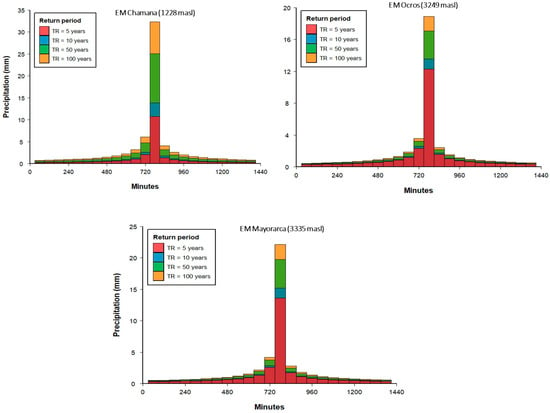
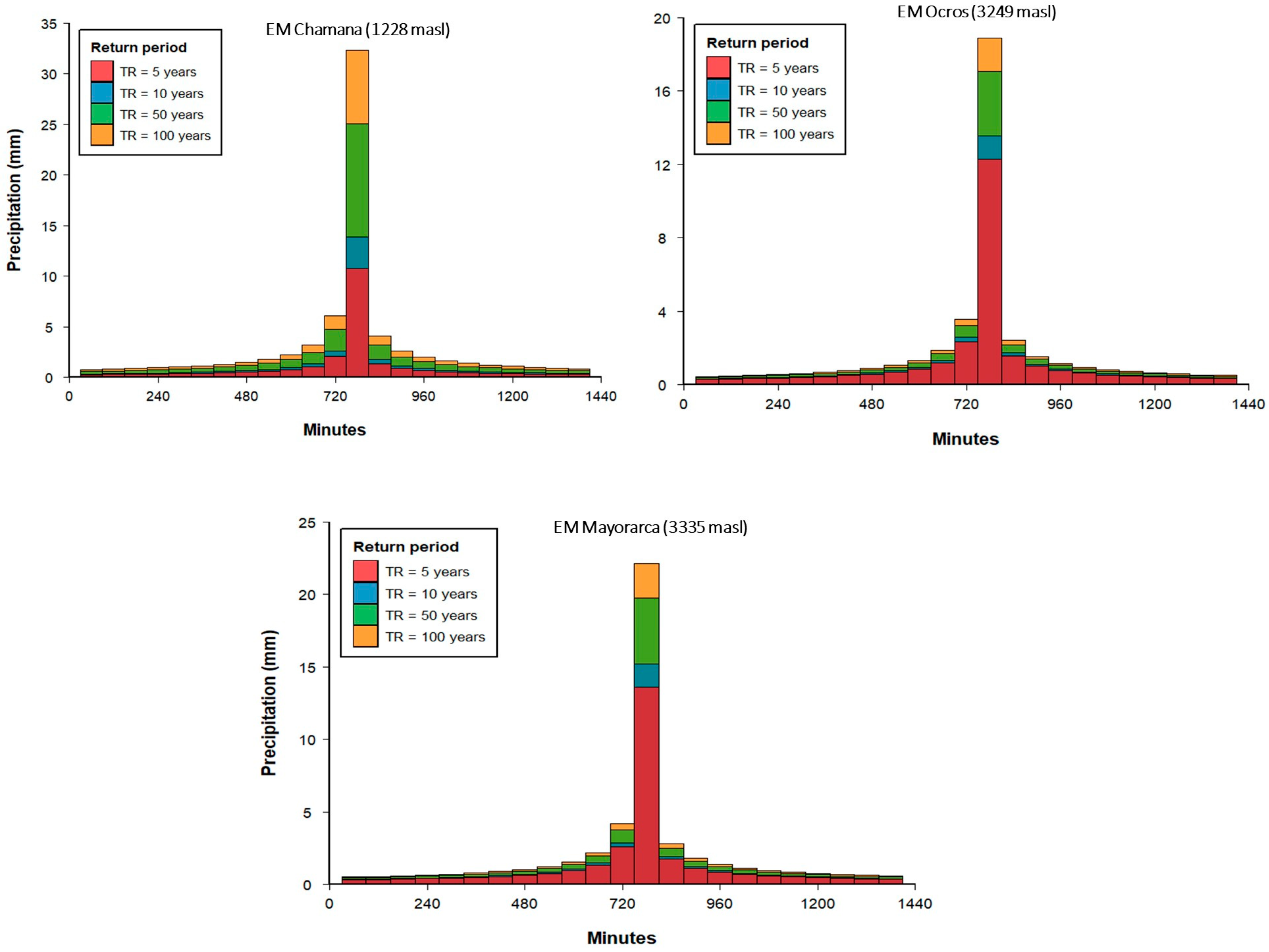
The results of the extreme rainfall analysis (24 h maximum precipitation) for each station are presented in Figure 4. Intensity–duration–frequency curves and design storm hyetographs for return periods of 5, 10, 50, and 100 years were derived for the Chamana (a), Ocros (b), and Mayorarca (c) stations.

Figure 4. Hyetographs of 24 h maximum precipitation for different return periods at meteorological stations.

The hyetographs show a consistent temporal pattern, with maximum intensities concentrated between 720 and 780 min (12–13 h) for all stations and return periods, reflecting the characteristic distribution of the alternating block method. A clear non-linear increase in maximum intensity with return period is observed at all stations; for example, at Chamana, the maximum hourly intensity increases from ~4.2 mm/h (5 years) to ~9.8 mm/h (100 years). Furthermore, a marked spatial gradient is evident: the lowland station (Chamana, 1228 masl.) presents consistently higher intensities than the high-Andean stations (Mayorarca, 3335 masl.; Ocros, 3249 masl.), consistent with the orographic control of precipitation documented in the region.

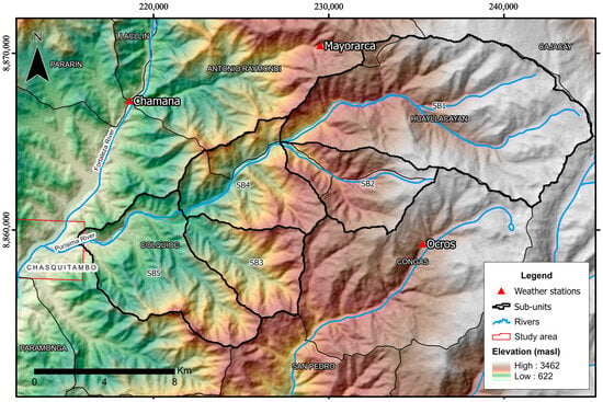
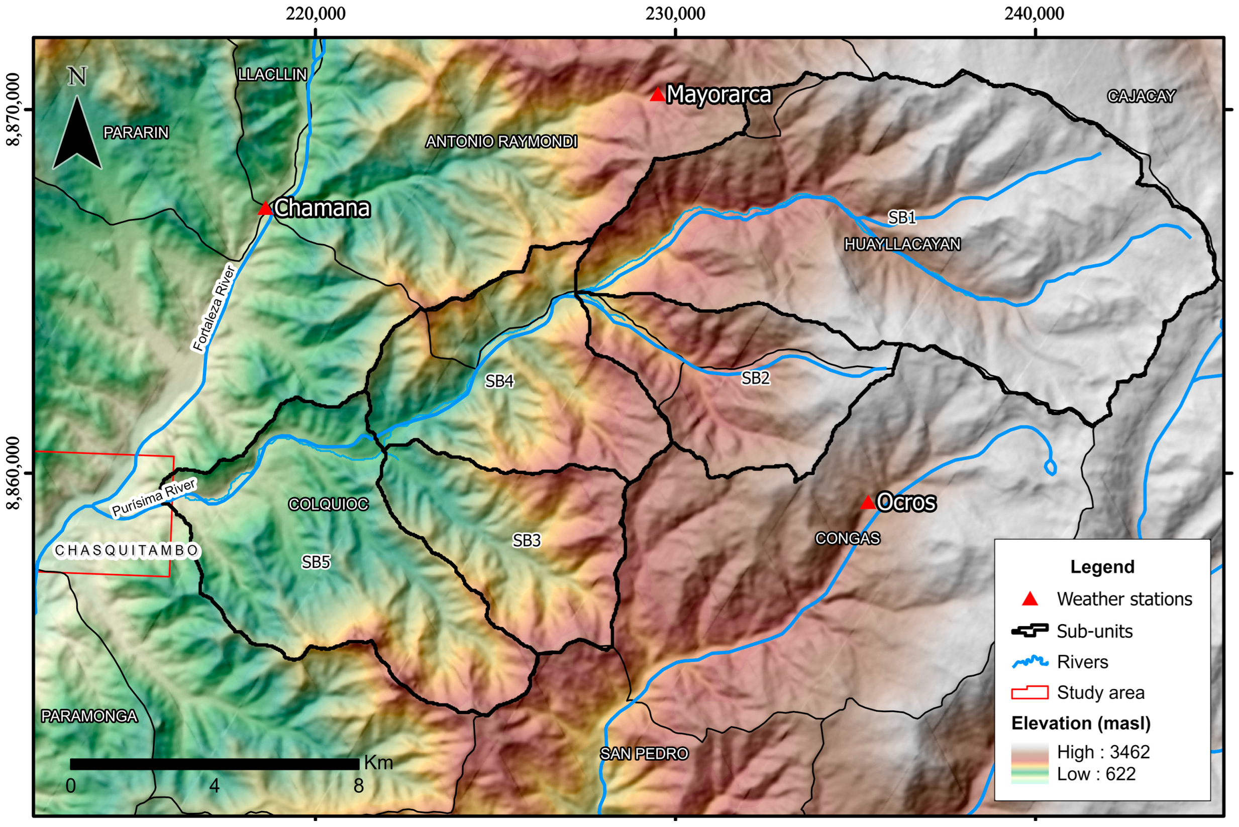
To estimate design flood peaks for the debris flow modeling, the Purísima watershed was subdivided into five sub-units (sub-catchments), each identified as having a high runoff generation potential (Figure 5). This subdivision was based on the geomorphological variability of the basin (slope, land cover, soil type). Table 5 summarizes the drainage network parameters for the five analytical sub-units (SB1–SB5) delineated within the Purísima basin; these sub-units exhibit notable variability in their morphometric characteristics, reflecting the terrain. The calculated times of concentration vary accordingly, ranging from 121.8 min (SB4) to 209.6 min (SB3), consistent with the overall basin concentration time (128 min) and aligned with the critical storm duration identified in the hyetograph analysis (12–13 h). The Curve Numbers (CNs) indicate a moderate to high runoff potential, with higher values in sub-units characterized by steeper slopes and less permeable soils. Hyetographs for each sub-unit (corresponding to each return period) were obtained by spatially interpolating the station hyetographs using the Thiessen polygon method.

Figure 5. Schematic of the Purísima watershed divided into five analytical sub-units for runoff modeling.

Table 5. Hydrographic network parameters of the analytical sub-units.

Sub-Unit	Morphometric Parameters
	Area (km2)	Main Channel Length (km)	Avg. Slope (%)	Time of Concentration (min)	Curve Number (CN)
SB1	103.14	22.96	12.55	167.84	85
SB2	26.95	11.05	13.17	157.92	65
SB3	34.01	11.72	8.23	209.61	65
SB4	25.56	9.45	10.25	121.83	75
SB5	45.34	15.83	6.98	194.09	80

Sub-units 1 and 5 encompass primarily cultivated lands without special soil conservation practices, characterized by shallow loamy sand soils that exhibit moderate infiltration when wet. In contrast, sub-units 2, 3, and 4 consist of forested or grassland areas (with relatively poor-quality grass cover) and similarly moderate infiltration capacity.

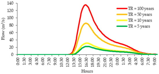
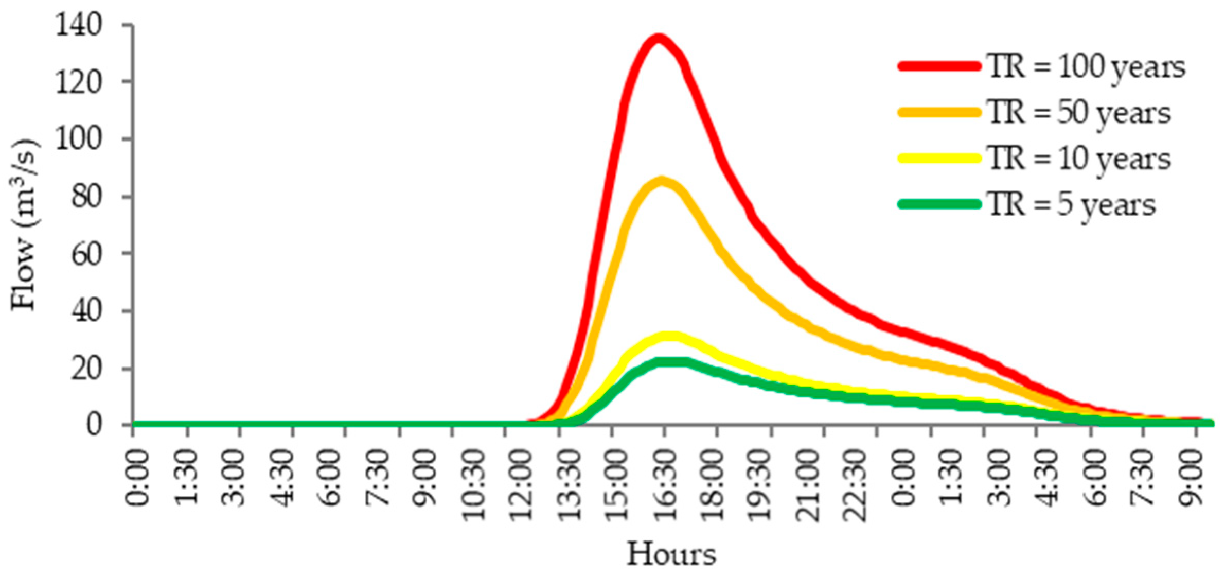
Using the above subdivision, rainfall–runoff simulations were carried out for each return period. Figure 6 shows the resulting unit hydrographs (runoff response) for the Purísima watershed. The peak discharges range from approximately 22 m³/s for a 5-year event to 135 m³/s for a 100-year event. These peak flows occur in the late afternoon (around 17:00 h) for all scenarios, given the rainfall timing in the design storms.

Figure 6. Unit hydrographs of peak outflow for the Purísima watershed under different TR (returnperiod) rainstorms.

3.3. Calibration Against 2023 Debris Flow Marks

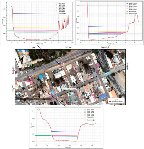
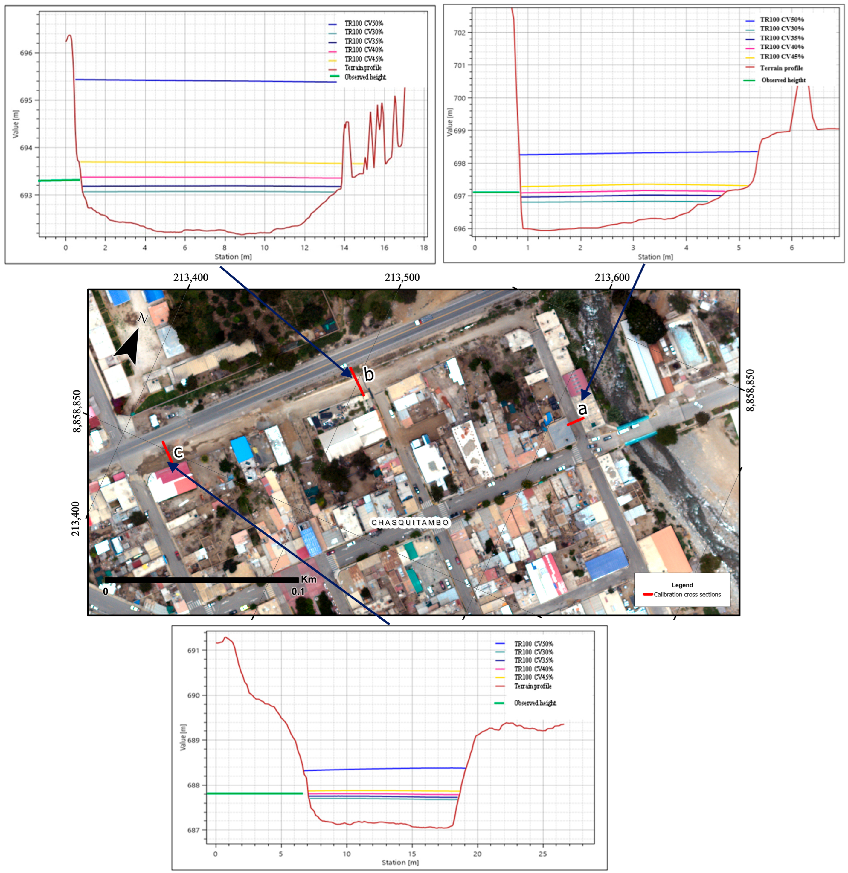
A calibration of the numerical model was performed using field observations from the 12 March 2023 event. Flow depth marks from that event were measured at three reference cross-sections in the affected area. These observed high-water marks were compared to the simulated flow depths for a 100-year return period event under various assumed sediment concentrations in the model. The goal was to find which sediment concentration produced model results closest to the real event measurements.

Figure 7 presents the longitudinal profiles of modeled flow depths at the three calibration cross-sections (a, b, and c) for sediment concentrations ranging from 30% to 50% compared with the elevations of the observed debris flow stage lines and marks recorded in the field. The results reveal that lower concentrations (30–35%) consistently underestimate the observed flow depth. Conversely, higher concentrations (45–50%) overestimate flow depth, with the 50% scenario producing substantial positive deviations. The consistent performance across multiple cross-sections, spaced 100–150 m apart along the flow path, demonstrates the model’s ability to reproduce not only the maximum flow depth but also the longitudinal profile.

Figure 7. Comparison of modeled flow depths to observed high-water marks at three calibration cross-sections in Chasquitambo (for the 100-year scenario under different sediment concentration assumptions).

According to the calibration results (Table 6), comparing the simulated and observed maximum flow elevations at the three cross-sections (a, b, c) for sediment concentrations ranging from 30% to 50%, the model scenario with a 40% volumetric sediment concentration provided the best match to observed flow depths. At 40% C_v, the differences between modeled and observed peak flow elevations were minimal (–0.02 m, –0.02 m, and +0.01 m at sections a, b, and c, respectively), well within the accuracy of the field measurements. This yields a root mean square error (RMSE) of approximately 0.017 m, a mean absolute error (MAE) of 0.017 m, and a negligible mean relative error (0.0024%). These very small errors indicate an excellent fit, validating that the model can accurately reproduce the real event when using a 40% sediment concentration. This calibrated value (Cv = 40%) is event-specific, representing a model adjustment tailored to the particular conditions of the March 2023 extreme event. Therefore, a C_v of 40% was adopted for all scenario simulations (as reported in Section 3.4), as it best represents the actual debris flow conditions observed.

Table 6. Model calibration results at three cross-sections (a, b, c) for varying sediment concentrations.

Sediment Conc. (% Vol)	Section	Max. Modeled Elev. (masl)	Observed Elev. (masl)	Difference (m)
30	a	696.78	697.12	−0.34
35		696.90	697.12	−0.22
40		697.10	697.12	−0.02 *
45		697.17	697.12	0.05
50		698.19	697.12	1.07
30	b	693.11	693.38	−0.27
35		693.20	693.38	−0.18
40		693.40	693.38	0.02 *
45		693.50	693.38	0.12
50		695.41	693.38	2.03
30	c	687.68	687.80	−0.12
35		687.73	687.80	−0.07
40		687.79	687.80	−0.01 *
45		687.87	687.80	0.07
50		688.38	687.80	0.58

(*) Is the modeled scenario closest to what was observed.

Overall, these findings provide critical insight for disaster risk management. The calibrated model, with its verified accuracy, can reliably simulate debris flow scenarios of varying magnitudes. The scenario analyses (Section 3.4) at both local (Chasquitambo) and broader watershed scales furnish essential information for stakeholders to develop mitigation strategies. These strategies can be formulated along prospective (risk prevention), corrective (mitigation of existing risk), and reactive (emergency response) lines, with the aim of safeguarding lives, socioeconomic activities, and public infrastructure.

3.4. Debris Flow Modeling

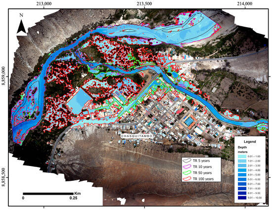
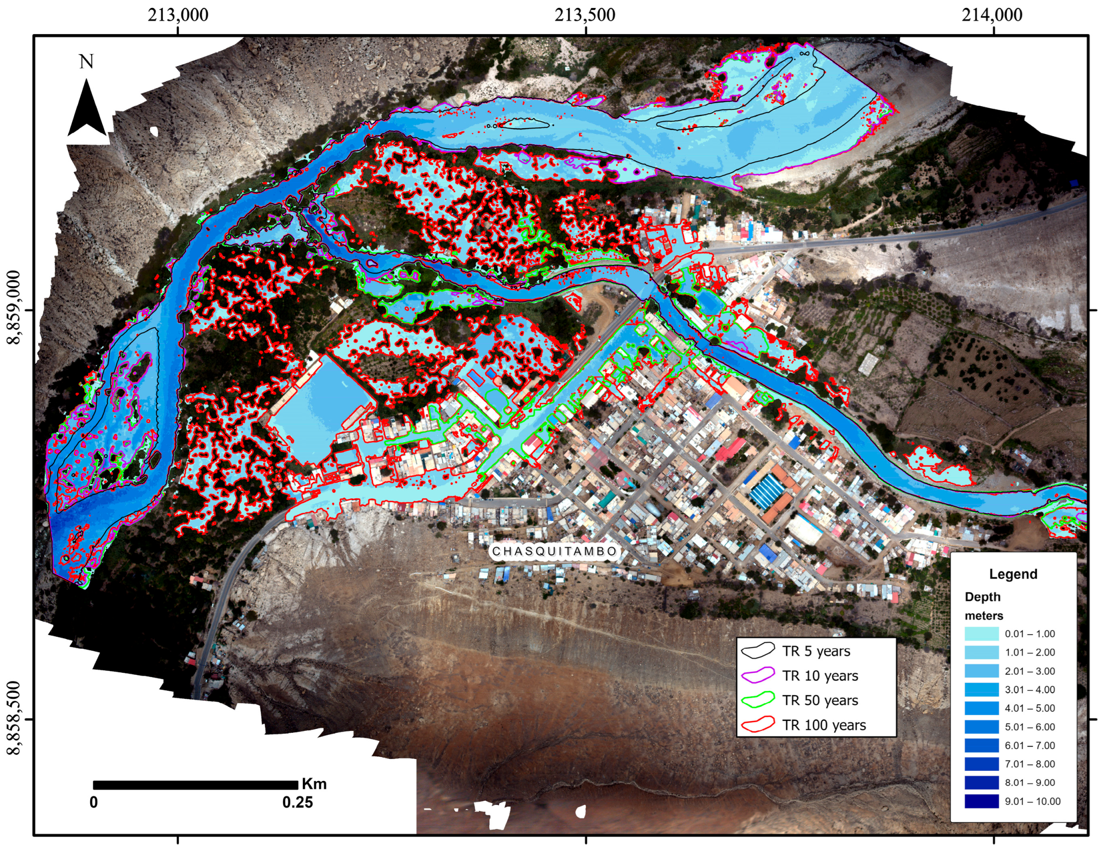
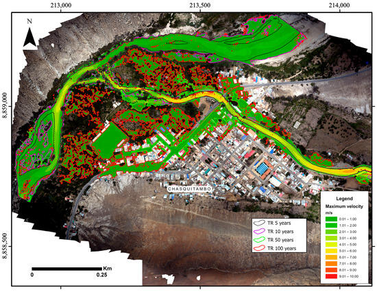
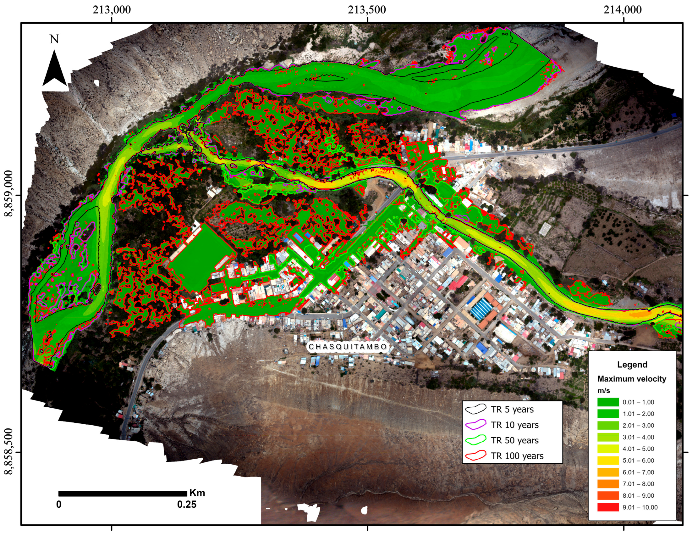
For the 2D HEC-RAS debris flow model, the computational mesh and model setup are described in Section 2.5 above. Figure 8 and Figure 9 (depth and velocity, respectively) illustrate the simulated debris flow propagation for all scenarios, describing their implications below.

Figure 8. Maximum flow depths for the study scenarios.

Figure 9. Maximum flow velocities for the study scenarios.

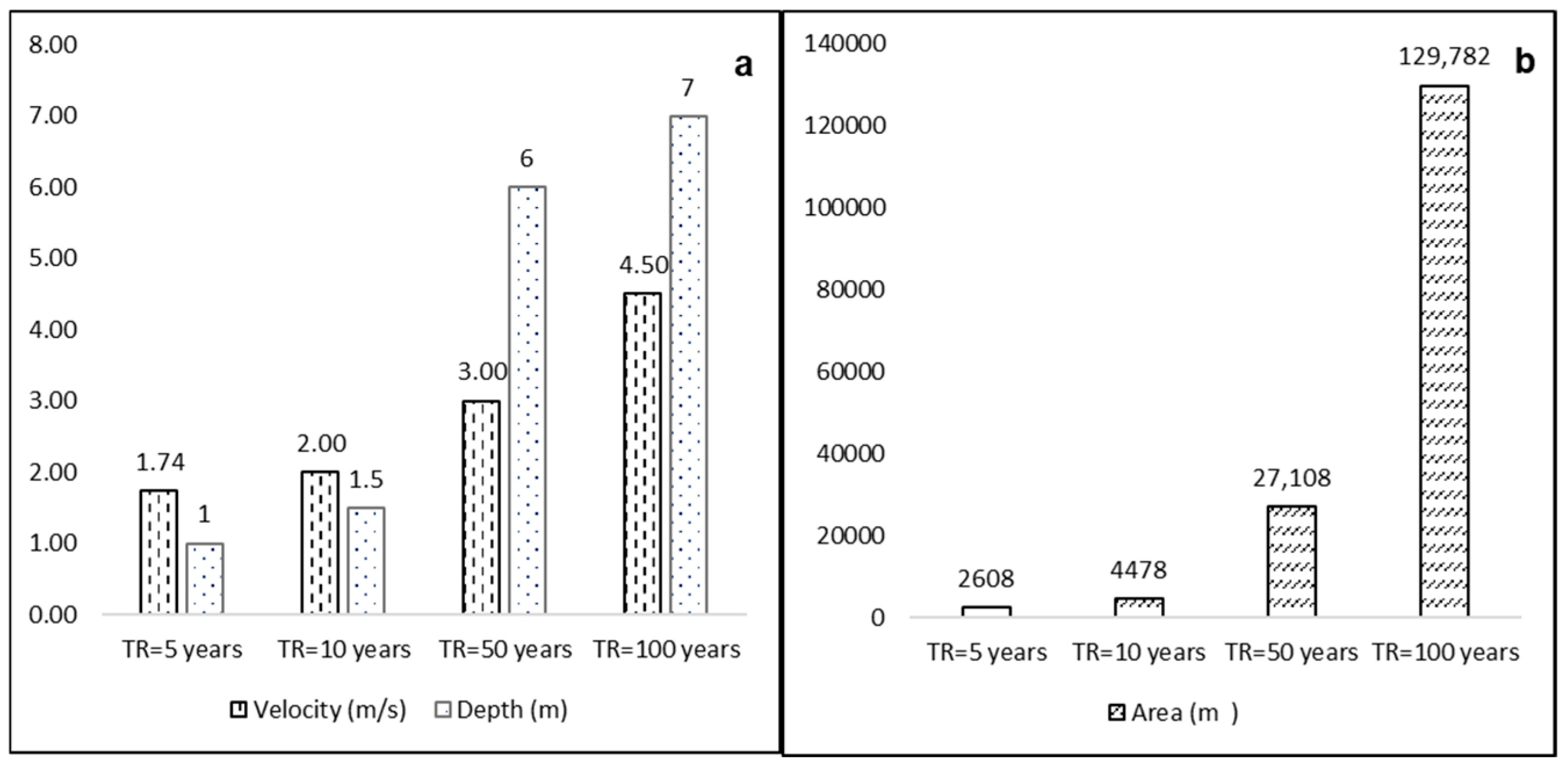
A 5-year scenario: Under this lower-magnitude scenario, the model projects that debris flow inundation is mostly confined to the confluence area of the Purísima and Fortaleza rivers. Approximately 2608 m² of agricultural land (farmland near the river confluence) would be affected. Predicted flow depths in that area range from 0.1 to 1.0 m, and flow velocities reach up to 1.74 m/s. Structural damage in this scenario is minimal, although agricultural fields would be impacted by deposition and erosion.

A 10-year scenario: The extent of inundation increases modestly compared to the 5-year event. The model indicates roughly 4478 m² of agricultural land (at the river confluence and slightly further downstream) could be inundated, with flow depths of 0.1–1.5 m and velocities up to 2.00 m/s. Again, the primary impacts are on agricultural plots adjacent to the riverbanks. No significant infrastructure damage is projected beyond some possible effects on unpaved rural roads or minor structures near the flow path.

A 50-year scenario: As the return period increases to 50 years, the predicted impacts grow substantially. The model results (summarized in Figure 8 and Figure 9) indicate that approximately 12,881 m² of agricultural land could be affected, with debris flow depths of 5–7 m in the main channel and up to 2–3 m in inundated farmland. Maximum velocities reach about 2.4 m/s. In the urban area of Chasquitambo, which lies on the alluvial fan, the model projects that around 14,227 m² could be flooded by the debris flow to depths of 0.1–3.0 m (primarily at the fringes of the main flow). The average flow velocity in the inundated town area would be 0.5 m/s (much lower than in the channel due to spreading of the flow). Even at these moderate velocities, the presence of a large sediment load can cause considerable damage.

At the 50-year intensity, significant disruption to critical services is expected; potable water supply lines, sewerage, and electricity networks in the affected area could be damaged. The simulation estimates potential structural impacts on 38 houses, two small bridges, one school, and roughly 738 m of road in and around Chasquitambo (mainly due to burial by debris or undermining of foundations), as shown in Figure 8 and Figure 9.

A 100-year scenario: The 100-year return period scenario represents an event of similar magnitude to the Cyclone Yaku 2023 disaster. The inundation extent and impact are dramatically larger. Approximately 73,327 m² of agricultural land could be affected, with flow depths of 5–7 m and velocities up to 4.5 m/s in the channel and immediately adjacent floodplain. In the town, roughly 56,544 m² (about 5.65 hectares) of urban area may be covered by debris flow deposits ranging from 1 to 3 m in depth. Flow velocities in the urban inundation zone are in the 0.5–2 m/s range. These conditions would likely result in severe damage; the model projects potential impact to around 144 houses, two bridges, one school, one police station, 32 commercial establishments, and approximately 1386 m of roads. Essentially, a 100-year event could inundate a significant portion of Chasquitambo with debris, causing widespread destruction of buildings and infrastructure and posing a serious threat to lives.

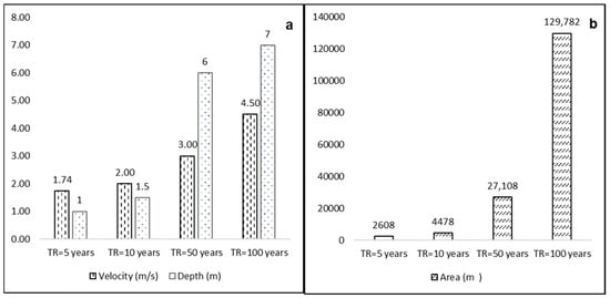
To synthesize the scenario results for the four return periods, Figure 10 and Table 7 summarize how the key impact metrics scale with return period, revealing the existence of a direct and highly non-linear relationship between the triggering rainfall return period and the debris flow magnitude. The peak discharge of the mixture (40% sediment) increases from 37.33 m³/s (5 years) to 225.67 m³/s (100 years)—a sixfold increase—while the flooded area expands dramatically from 2608 m² to 129,872 m², an increase of nearly 50 times. The maximum flow velocity progressively increases from 1.74 m/s to 4.50 m/s, and the maximum depth increases from approximately 1.5 m to 7.0 m.

Figure 10. Comparison of simulated debris flow severity across return periods. (a) Maximum velocities (m/s) and maximum flow depths (m) for each scenario; (b) inundated area (affected area in m²) for each scenario.

Table 7. Summary of simulation results for different return-period scenarios.

Metric	5-Year	10-Year	50-Year	100-Year
Peak discharge (water only, m3/s)	22.40	31.30	85.50	135.40
Peak discharge (mixture, 40% Cv, m3/s)	37.33	52.17	142.50	225.67
Inundated area (m2)	2608	4478	27,108	129,872
Velocity (m/s)	1.74	2.00	3.00	4.50
Max. flow velocity (m/s)	1.0	1.5	6.0	7.0
Primary affected elements	Cropland	Cropland	Cropland; 38 houses; local utilities; roads; bridges; school	Cropland; 144 houses; utilities; roads; bridges; school; police station; shops; stadium

This non-linear scaling has direct implications for hazard assessment; the 50- and 100-year scenarios (discharges > 85 m³/s) are capable of causing severe damage to urban infrastructure, affecting 38 and 148 dwellings, respectively, in addition to roads, bridges, schools, and critical buildings, such as the police station and the stadium. In contrast, the 5- and 10-year events (discharges < 52 m³/s) are mainly limited to agricultural areas and the channel, producing localized impacts. These results demonstrate that longer return periods are associated with more severe debris flows and, consequently, a much greater damage potential.

4. Discussion

The debris flow rheological model of O’Brien and Julien (Bingham-type formulation) was used with parameters from the Glenwood sample 2 dataset. This choice was justified by the local soil composition (predominantly sandy-gravelly with 16% fines). For the calibrated model at 40% sediment concentration by volume, the yield stress and dynamic viscosity were 10.704 Pa and 0.077 Pa·s, respectively, which fall in a typical range for such flows. This similarity is supported by previous studies [33,37], which note that hyperconcentrated flows occurring on natural slopes require a significant fine-particle content and a heterogeneous grain-size distribution to develop the cohesive properties that influence rheological behavior. Moreover, research by Julien [38] highlights that the fine fraction directly controls the apparent viscosity, yield stress, and overall flow behavior of debris flows. In our calibrated model (40% sediment concentration), the yield stress was 10.704 Pa and the dynamic viscosity was 0.077 Pa·s. These values are consistent with those obtained by other authors [21] for debris flows in arid regions of Peru under similar conditions. According to Takahashi [39], values in this range are optimal for simulating debris flows. Furthermore, Scotto [15] indicates that typical yield stress values for debris flows range between 10 and 15 Pa, and the viscosity we obtained aligns with typical characteristics of these flows [40]. Consequently, as pointed out by Rickenmann [41], the combination of yield stress and viscosity (along with other rheological parameters) significantly influences debris flow velocity, travel distance, sediment deposition patterns, and interactions with obstacles.

Selecting an appropriate statistical distribution for extreme rainfall is essential to avoid under- or overestimation of design events [42]. Given the stochastic nature of precipitation, it is necessary to evaluate multiple candidate distributions [43]. In this study, based on goodness-of-fit testing, a Log-Normal distribution was selected for the Chamana and Ocros stations, and a Log-Pearson Type III distribution was selected for Mayorarca. These distributions provided the best fit for annual maximum daily rainfall at each station (per the Kolmogorov–Smirnov test). The resulting IDF curves derived from these distributions are valuable for risk analysis, as they characterize the expected intensity of extreme rains across durations and frequencies [44], providing operational rainfall thresholds. These thresholds are applicable as site-specific local values [45], but their derivation from extreme events is reliable and conservative for lower-magnitude events [46]. This is consistent with the obtained value (20 mm/24 h), which was derived from extreme scenarios. Additionally, the alternate block hyetographs generated for each return period offer a realistic temporal representation of extreme storm events, compensating for the lack of sub-daily rainfall data [47], which is a crucial input for debris flow simulation [34]. It should be noted that the use of daily total rainfall, even when distributed into shorter duration intervals using synthetic methods, entails uncertainties in the exact timing of the peak discharge [45]. However, the applied pattern provides a temporally coherent representation, consistent with typical extreme events, approximating the worst possible scenario within the analyzed return periods.

The morphometric characteristics of the Purísima basin—particularly its steep slopes and relatively short concentration times—indicate a high potential for rapid runoff generation and, consequently, debris flow initiation [48]. The unit hydrographs for different return periods exhibit a marked increase in peak discharge as the return period increases. Notably, modeled flows exceeding 85 m³/s (associated with return periods ≥50 years) are capable of causing severe damage in urban areas, whereas smaller peak discharges tend to produce impacts largely confined to agricultural zones. This behavior underscores a key point in debris flow risk assessment: low-frequency, high-magnitude events (rare but very intense storms) can have catastrophic consequences in vulnerable areas [49].

The HEC-RAS model does have certain limitations in representing debris flows, especially when using the O’Brien and Julien rheological formulation. These limitations stem from the simplified representation of interactions between solid particles and fluid, the assumption of constant sediment concentration during transport [37,38], and the omission of dynamic erosion–deposition processes on complex topography [25]. To account for these, we calibrated the model to ensure the simulations remain reliable. Calibration (by matching simulated vs. observed flow depths) proved effective, as discussed above, although using the calibrated values for smaller events results in a prudent overestimation of the inundated areas; this constitutes a conservative and prudent approach [46], which collectively offsets the limitations inherent in using a fixed Manning’s and omitting complex dynamic processes [35]. It is worth noting that debris flow erosion typically initiates on slopes steeper than 10% [43]. In our case, the main at-risk area (the town) lies on slopes gentler than 10%, implying that most erosion likely occurred upstream in the steeper ravines. By the time the flow reached Chasquitambo, it became predominantly depositional, which is consistent with our model showing deposition depths of 1–3 m in town. Within the modeling framework and chosen rheology, the simulations are considered representative of actual behavior under these conditions. Similar approaches by other studies [7,21,50] using the O’Brien and Julien model (in HEC-RAS or in other software, like FLO-2D pro) have reported comparable success in simulating debris flow events.

The propagation models for the smaller events (5- and 10-year) revealed only moderate impacts, as expected for lower-magnitude flows [51]. These more frequent events primarily threaten agricultural infrastructure (e.g., canals, fields) and light structures near channel banks, while causing little damage to well-built structures [52]. In contrast, the 50- and 100-year scenarios showed severe impacts, including complete loss of crops and substantial structural damage [53,54], which pose serious threats to human life. This dichotomy between frequent–minor and rare–catastrophic events is important for local risk management strategies.

Although the numerical values reported (discharges, flow depths, flood areas) are site-specific, the observed pattern of a strongly non-linear increase in extent and impact metrics with rainfall severity is consistent with the international literature on debris flows [55]. This critical amplification effect, recently documented in the Alps, Himalayas, and Taiwan [56], is confirmed here for the Peruvian Andes, reinforcing the need for scenario-based planning that considers high-magnitude events [55]. Furthermore, the operational threshold proposed in this study aligns with recent approaches that couple rainfall thresholds with early warning system performance in data-limited basins, demonstrating the constitution of an effective risk reduction strategy where data are scarce [57], with successful experiences such as in Glenwood Canyon (Colorado, USA) [58]. Consequently, the main transferable contribution is the comprehensive and data-efficient workflow (event documentation, high-resolution topography, calibrated 2D modeling, scenario-based mapping, and operational thresholds), replicable in other data-limited mountain basins to derive local thresholds and priority protection zones, thereby contributing to disaster risk reduction where conventional approaches are unfeasible [55,57].

Our numerical simulations underscore an urgent need to implement both structural and non-structural risk management measures [59]. Structural measures should aim to dissipate or divert debris flows; for example, via retention dams, check dams, diversion channels, and reinforced retaining walls in critical spots [60]. Notably, previous studies have demonstrated that such interventions can reduce debris flow velocity by up to 75%, greatly mitigating impact forces and runout extent (e.g., strategic check dams reducing flow energy) [61]. Non-structural measures should complement these physical defenses. For instance, community-based early warning systems and public education campaigns have been shown to reduce vulnerability by about 40% and disaster mortality by around 50% in similar contexts [62].

Furthermore, climate projections for this region suggest that extreme rainfall events may become more intense and frequent in the future [63]. This reinforces the need to incorporate nature-based solutions into the mitigation portfolio. Such solutions include reforestation with deep-rooted native species and slope stabilization through bioengineering. These approaches help address the root causes of debris flows by reducing soil erosion and improving water infiltration, thereby lowering runoff and sediment yield [63]. In essence, combining hard engineering with ecosystem-based measures can provide sustainable, multi-functional protection against debris flow hazards.

Within the broader context of disaster risk management for Chasquitambo, our model outputs suggest operational warning thresholds. Specifically, approximately 20 mm of accumulated rainfall in 24 h (which corresponds to about a 50-year return period storm) should trigger a red alert for the area, as it is likely to produce debris flows capable of reaching and impacting the town. Lesser rainfall events (below this threshold) can be classified as a yellow alert, indicating that impacts would primarily be limited to agricultural zones and river channels, without major urban damage. This threshold-based warning can enable timely evacuations and activation of emergency protocols. Lastly, it is crucial that structural protection works and evacuation plans prioritize the zones of highest impact identified in our 50-year and 100-year simulations (see Figure 8 for spatial impact extents).

5. Conclusions

Based on a calibration using the Cyclone Yaku event (12 March 2023) and an ultra-high-resolution drone-derived DEM (0.12 m), debris flow hazard was quantified for design storms with return periods of 5, 10, 50, and 100 years. The calibrated model (sediment concentration 40%) reproduces the observed flow depths with sub-decimetric accuracy (±0.02 m), demonstrating that even a single documented extreme event, when combined with high-resolution topography, can provide a robust hazard assessment. This finding is particularly relevant for data-limited regions where conventional long-term records are unavailable.

The simulations reveal a strongly non-linear relationship between rainfall severity and debris flow impact, ranging from impacts confined to the channel and agricultural areas (TR 5–10 years) to severe urban affectation with maximum depths of ~7 m and peak velocities of ~4.5 m/s in the 100-year scenario. This non-linearity implies that events with long recurrence intervals concentrate a substantial portion of the risk and must be explicitly considered in land-use planning, emergency protocols, and early warning systems.

An operational rainfall threshold of approximately 20 mm/24 h is proposed to activate a maximum alert state and trigger preparedness actions in Chasquitambo; below this level, significantly lower and mostly non-urban impacts are expected. Applicable year-round, its significance is greater during the wet season when antecedent soil moisture amplifies the runoff response. Nevertheless, it provides a temporally coherent and conservative representation of extreme storm events for data-limited contexts where sub-daily records are not available. This threshold should be periodically updated as new events and improved rainfall data become available, and its application requires clear community protocols integrated with local early warning systems.

Although the numerical values of the hazard metrics and the rainfall threshold are site-specific, the proposed workflow—comprising event reconstruction, high-resolution topography, calibrated 2D modeling, and scenario-based mapping—is transferable to other data-limited mountain basins for deriving local thresholds and priority protection zones.

References

- Gariano, S.L.; Guzzetti, F. Landslides in a changing climate. Earth Sci. Rev. 2016, 162, 227–252. [Google Scholar] [CrossRef] [Scilit]
- UNDRR. El Costo Humano de los Desastres: Una Visión General de Los Últimos 20 Años (2000–2019); United Nations Office for Disaster Risk Reduction: Geneva, Switzerland, 2020. [Google Scholar]
- INDECI. Compendio Estadístico; Instituto Nacional de Defensa Civil: Lima, Perú, 2021.
- INDECI. Compendio Estadístico-Gestión Reactiva; Instituto Nacional de Defensa Civil: Lima, Perú, 2023.
- Díaz-Salas, A.M.; Guevara-Pérez, E.; Vidal-Moreno, J.D. Numerical modeling of a debris flow associated with a dam break in the Quillcay sub basin, Ancash, Peru. Rev. Ing. UC 2021, 28, 35–46. [Google Scholar]
- Alvarez, M.; Mastrantonio, L.; Moreiras, S. Análisis de susceptibilidad de flujos de detritos en el Parque Provincial Aconcagua, Mendoza, Argentina. Rev. Fac. Cienc. Agrar. 2019, 51, 177–191. [Google Scholar]
- IGP. Aspectos Geodinámicos y Simulación Numérica de Flujo de Detritos en la Quebrada Záparo; Instituto Geofísico del Perú: Lima, Perú, 2021.
- Suzuki, T.; Hotta, N.; Tsunetaka, H.; Sakai, Y. Application of an MPS-based model to the process of debris-flow deposition on alluvial fans. In Proceedings of the 7th International Conference on Debris-Flow Hazards Mitigation, Golden, CO, USA, 10–13 June 2019; pp. 871–878. [Google Scholar]
- Xu, H.; Su, P.; Chen, Q.; Liu, F.; Zhou, Q.; Liu, L. Susceptibility areas identification and risk assessment of debris flow using the Flow-R model: A case study of Basu County of Tibet. Geoenviron. Disasters 2022, 9, 2–21. [Google Scholar] [CrossRef] [Scilit]
- You, Y.; Zhou, N.; Wang, Y. Comparative study of desertification control policies and regulations in representative countries of the Belt and Road Initiative. Glob. Ecol. Conserv. 2021, 27, e01577. [Google Scholar] [CrossRef] [Scilit]
- Takebayashi, H.; Fujita, M.; Ohgushi, K. Numerical modeling of debris flows using basic equations in generalized curvilinear coordinate system and its application to debris flows in Kinryu River Basin in Saga City, Japan. J. Hydrol. 2022, 615, 128636. [Google Scholar] [CrossRef] [Scilit]
- Bolliger, D.; Schlunegger, F.; McArdell, B.W. Comparison of debris flow observations, including fine-sediment grain size and composition and runout model results, at Illgraben, Swiss Alps. Nat. Hazards Earth Syst. Sci. 2024, 24, 1035–1049. [Google Scholar] [CrossRef] [Scilit]
- Abraham, M.T.; Satyam, N.; Pradhan, B.; Tian, H. Debris flow simulation 2D (DFS 2D): Numerical modelling of debris flows and calibration of friction parameters. J. Rock Mech. Geotech. Eng. 2022, 14, 1747–1760. [Google Scholar] [CrossRef] [Scilit]
- Pandey, B.R.; Knoblauch, H.; Zenz, G. Potential Dam Breach Flood Assessment with the 2D Diffusion and Full Dynamic Wave Equations Using a Hydrologic Engineering Center-River Analysis System. Water 2024, 16, 277. [Google Scholar] [CrossRef] [Scilit]
- Rickenmann, D.; Laigle, D.; McArdell, B.W.; Hübl, J. Comparison of 2D debris-flow simulation models with field events. Comput. Geosci. 2006, 10, 241–264. [Google Scholar] [CrossRef] [Scilit]
- Ioriatti, E.; Reguzzoni, M.; Reguzzoni, E.; Schimmel, A.; Beretta, L.; Ceriani, M.; Berti, M. Identification of rainfall thresholds for debris-flow occurrence through field monitoring data. Nat. Hazards Earth Syst. Sci. 2025, 25, 4941–4959. [Google Scholar] [CrossRef] [Scilit]
- Caine, N. The Rainfall Intensity: Duration Control of Shallow Landslides and Debris Flows. Geogr. Ann. Ser. A Phys. Geogr. 1980, 62, 23–27. [Google Scholar]
- Marra, F.; Nikolopoulos, E.I.; Creutin, J.D.; Borga, M. Radar rainfall estimation for the identification of debris-flow occurrence thresholds. J. Hydrol. 2014, 519, 1607–1619. [Google Scholar] [CrossRef] [Scilit]
- Marra, F.; Destro, E.; Nikolopoulos, E.I.; Zoccatelli, D.; Creutin, J.D.; Guzzetti, F.; Borga, M. Impact of rainfall spatial aggregation on the identification of debris flow occurrence thresholds. Hydrol. Earth Syst. Sci. 2017, 21, 4525–4532. [Google Scholar] [CrossRef] [Scilit]
- Li, Y.; Wang, M.; Ma, F.; Zhang, J.; Li, G.; Meng, X.; Chen, G.; Yue, D.; Guo, F.; Zhao, Y. Constructing Rainfall Threshold for Debris Flows of a Defined Hazardous Magnitude. Remote Sens. 2024, 16, 1265. [Google Scholar] [CrossRef] [Scilit]
- Asencios, H. Flujo de Escombros Desencadenado Por Lluvias Extremas en la Quebrada Pedregal, Chosica; Subdirección de Estudios e Investigaciones Hidrológicas del Servicio Nacional de Meteorología e Hidrología del Perú: Lima, Perú, 2020; pp. 22–30.
- Mueting, A.; Bookhagen, B.; Strecker, M.R. Using high-resolution DEMs for debris flow detection based on topographic signatures: A case study in the Quebrada del Toro, NW Argentina. In Proceedings of the EGU General Assembly 2020, Online, 4–8 May 2020. EGU2020-4236. [Google Scholar]
- Chacon Lima, D.; Huarca Pulcha, A.; Torrejon Llamoca, M.; Noriega Aquise, G.Y.; Espinoza Vigil, A.J. Hydraulic Modeling of Newtonian and Non-Newtonian Debris Flows in Alluvial Fans: A Case Study in the Peruvian Andes. Water 2025, 17, 2150. [Google Scholar] [CrossRef] [Scilit]
- Gómez Cardona, F.; Aristizábal Giraldo, E.; Mergili, M. Modelling debris flood propagation in scarce data terrain, case study in the Colombian Andes. J. S. Am. Earth Sci. 2025, 165, 105660. [Google Scholar] [CrossRef] [Scilit]
- Gibson, S.; Sánchez, A. HEC-RAS, Mud and Debris Flow Manual; US Army Corps of Engineers: Davis, CA, USA, 2020.
- Iglesias, I.; Echevarría, P.; Montes, I.; Segura, B.; Quispe, W.; Pasapera, J.; Chamorro, A. Forcings and Evolution of the 2017 Coastal El Niño Off Northern Peru and Ecuador. Front. Mar. Sci. 2018, 5, 367. [Google Scholar] [CrossRef] [Scilit]
- Manay, R.; Sulca, J.; Montes, I.; Castillón, F. Afloramiento costero peruano en presencia del ciclón Yaku durante marzo de 2023. Bol. Cient. Niño 2023, 10, 12–15. [Google Scholar]
- Bograd, S.J.; Jacox, M.G.; Hazen, E.L.; Lovecchio, E.; Montes, I.; Pozo Buil, M.; Shannon, L.J.; Sydeman, W.J.; Rykaczewski, R.R. Climate Change Impacts on Eastern Boundary Upwelling Systems. Ann. Rev. Mar. Sci. 2023, 15, 303–328. [Google Scholar] [CrossRef] [Scilit]
- Takahashi, K.; Martínez, A.G. The very strong coastal El Niño in 1925 in the far-eastern Pacific. Clim. Dyn. 2017, 52, 7389–7415. [Google Scholar] [CrossRef] [Scilit]
- Timmermann, A.; An, S.I.; Kug, J.S.; Jin, F.F.; Cai, W.; Capotondi, A.; Cobb, K.M.; Lengaigne, M.; McPhaden, M.J.; Stuecker, M.F.; et al. El Niño-Southern Oscillation Complexity. Nature 2018, 559, 535–545. [Google Scholar] [CrossRef] [Scilit]
- ENFEN. El Niño/La Niña Costeros-IGP; Subdirección de Ciencias de la Atmósfera e Hidrósfera: Lima, Perú, 2012.
- SENAMHI. Boletín Climático Nacional: Monitoreo y Pronóstico del Clima; Servicio Nacional de Meteorología e Hidrología del Perú: Lima, Perú, 2023.
- Takahashi, T. Debris Flow Mechanics, Prediction and Countermeasures; Taylor & Francis: London, UK, 2007. [Google Scholar]
- Bezak, N.; Šraj, M.; Mikoš, M. Design Rainfall in Engineering Applications with Focus on the Design Discharge. In Engineering and Mathematical Topics in Rainfall; InTech: London, UK, 2018. [Google Scholar]
- O’Brien, J.S.; Julien, P.Y.; Fullerton, W.T. Two-Dimensional Water Flood and Mudflow Simulation. J. Hydraul. Eng. 1993, 119, 244–261. [Google Scholar] [CrossRef] [Scilit]
- O’Brien, J.S.; Julien, P.Y. Physical properties and mechanics of hyperconcentrated sediment flows. In Proceedings of the ASCE Specialty Conference on Delineation of Landslides, Flash Floods and Debris Flow Hazards, Logan, UT, USA, 14–15 June 1984; pp. 260–279. [Google Scholar]
- Hungr, O.; Leroueil, S.; Picarelli, L. The Varnes classification of landslide types, an update. Landslides 2013, 11, 167–194. [Google Scholar] [CrossRef] [Scilit]
- Iverson, R.M. The physics of debris flows. Rev. Geophys. 1997, 35, 245–296. [Google Scholar] [CrossRef] [Scilit]
- Scotto di Santolo, A.; Pellegrino, A.M.; Evangelista, A. Experimental study on the rheological behaviour of debris flow. Nat. Hazards Earth Syst. Sci. 2010, 10, 2507–2514. [Google Scholar] [CrossRef] [Scilit]
- Zhang, Z.; Liu, D.; Zhang, S.; He, S.; Chen, Z.; Li, Y. Insights From the Particle Impact Model Into the High-Frequency Seismic Signature of Debris Flows. Geophys. Res. Lett. 2021, 48, e2020GL088994. [Google Scholar] [CrossRef] [Scilit]
- Iverson, R.M.; George, D.L. Valid debris-flow models must avoid hot starts. In Proceedings of the 7th International Conference on Debris-Flow Hazards Mitigation, Golden, CO, USA, 10–13 June 2019; pp. 1–8. [Google Scholar]
- Staudinger, M.; Kauzlaric, M.; Mas, A.; Evin, G.; Hingray, B.; Viviroli, D. The role of antecedent conditions in translating precipitation events into extreme floods at catchment scale and in a large basin context. Nat. Hazards Earth Syst. Sci. 2025, 25, 247–265. [Google Scholar] [CrossRef] [Scilit]
- Frey, H.; Huggel, C.; Chisolm, R.E.; Bauder, A.; McArdell, B.W.; Cochachin, A. Multi-Source Glacial Lake Outburst Flood Hazard Assessment and Mapping for Huaraz, Cordillera Blanca, Peru. Front. Earth Sci. 2018, 6, 210. [Google Scholar] [CrossRef] [Scilit]
- Ragno, E.; AghaKouchak, A.; Love, C.A.; Cheng, L.; Vahedifard, F.; Lima, C.H.R. Quantifying Changes in Future Intensity-Duration-Frequency Curves Using Multimodel Ensemble Simulations. Water Resour. Res. 2018, 54, 1751–1764. [Google Scholar] [CrossRef] [Scilit]
- Nikolopoulos, E.I.; Crema, S.; Marchi, L.; Marra, F.; Guzzetti, F.; Borga, M. Impact of uncertainty in rainfall estimation on the identification of rainfall thresholds for debris flow occurrence. Geomorphology 2014, 221, 286–297. [Google Scholar] [CrossRef] [Scilit]
- Gregoretti, C.; Degetto, M.; Boreggio, M. GIS-based cell model for simulating debris flow runout on a fan. J. Hydrol. 2016, 534, 326–340. [Google Scholar] [CrossRef] [Scilit]
- Chow, V.T. Hidrología Aplicada; Martha Edana Suárez: Santa Fe de, Colombia, 1994. [Google Scholar]
- Borga, M.; Stoffel, M.; Marchi, L.; Marra, F.; Jakob, M. Hydrogeomorphic response to extreme rainfall in headwater systems: Flash floods and debris flows. J. Hydrol. 2014, 518, 194–205. [Google Scholar] [CrossRef] [Scilit]
- Destro, E.; Marra, F.; Nikolopoulos, E.I.; Zoccatelli, D.; Creutin, J.D.; Borga, M. Coupled prediction of flash flood response and debris flow occurrence: Application on an alpine extreme flood event. J. Hydrol. 2018, 558, 225–237. [Google Scholar] [CrossRef] [Scilit]
- López, M.; Mogrovejo, R. Análisis hidráulico del flujo de detritos en la quebrada Pedregal con FLO-2D-Chosica. In Proceedings of the X Congreso Nacional de Ingeniería Civil, Lima, Perú, 23 August 2023; p. 8. [Google Scholar]
- Kean, J.W.; Staley, D.M.; Lancaster, J.T.; Rengers, F.K.; Swanson, B.J.; Coe, J.A.; Hernandez, J.L.; Sigman, A.J.; Allstadt, K.E.; Lindsay, D.N. Inundation, flow dynamics, and damage in the 9 January 2018 Montecito debris-flow event, California, USA: Opportunities and challenges for post-wildfire risk assessment. Geosphere 2019, 15, 1140–1163. [Google Scholar] [CrossRef] [Scilit]
- Hürlimann, M.; Oorthuis, R.; Abancó, C.; Carleo, L.; Moya, J. Monitoring of rainfall and soil moisture at the Rebaixader catchment (Central Pyrenees). In Proceedings of the 7th International Conference on Debris-Flow Hazards Mitigation, Golden, CO, USA, 10–13 June 2019; pp. 1–8. [Google Scholar]
- Gregoretti, C.; Stancanelli, L.M.; Bernard, M.; Boreggio, M.; Degetto, M.; Lanzoni, S. Relevance of erosion processes when modelling in-channel gravel debris flows for efficient hazard assessment. J. Hydrol. 2019, 568, 575–591. [Google Scholar] [CrossRef] [Scilit]
- Marchi, L.; Cazorzi, F.; Arattano, M.; Cucchiaro, S.; Cavalli, M.; Crema, S. Debris flows recorded in the Moscardo catchment (Italian Alps) between 1990 and 2019. Nat. Hazards Earth Syst. Sci. 2021, 21, 87–97. [Google Scholar] [CrossRef] [Scilit]
- Jakob, M.; McDougall, S.; Santi, P.M. Advances in Debris-Flow Science and Practice; Springer: Cham, Switzerland, 2024. [Google Scholar]
- Harvey, E.L.; Fan, X.; Hales, T.C.; Li, Y.; Xu, Q.; Huang, R. The hazard of large debris flows. Sci. Adv. 2025, 11, 4625. [Google Scholar] [CrossRef] [Scilit] [PubMed]
- Ortenzi, S.; Massari, C.; Ciabatta, L.; Brocca, L.; Brunetti, M.T.; Peruccacci, S.; Guzzetti, F. Leveraging SMAP-Based Soil Moisture to Identify Runoff Thresholds on Flash Flood–Prone Basins in the Mediterranean Region. J. Hydrometeorol. 2025, 26, 975–990. [Google Scholar] [CrossRef] [Scilit]
- Rengers, F.K.; Kean, J.W.; Staley, D.M.; Oakley, N.S.; Lancaster, J.T.; McGuire, L.A.; Youberg, A.M.; Gorr, A.N. Forecast, Monitor, Adapt: A Multi-Agency Effort to Protect People during Postfire Debris Flows. GSA Today 2025, 35, 15–21. [Google Scholar] [CrossRef] [Scilit]
- CENEPRED. Manual Para la Evaluación de Riesgos Originados Por Fenómenos Naturales Versión 02; Centro Nacional de Estimación, Prevención y Reducción del Riesgo de Desastres: Lima, Perú, 2015.
- Nagl, G.; Hübl, J. A new debris flow monitoring barrier to measure debris flow impact/structure/ground interaction in the Gadria torrent. In Proceedings of the 5th International Conference on Debris-Flow Hazards Mitigation, Padua, Italy, 14–17 June 2017; pp. 1–8. [Google Scholar]
- Anderson, M.; Holcombe, E. Community-Based Landslide Risk Reduction; World Bank: Washington, DC, USA, 2013. [Google Scholar]
- Llacza Rodríguez, A.; Acuña, D.; Jara, J.; Cubas, F. Escenarios Climáticos al 2050 en el Perú: Cambios en el Clima Promedio; Servicio Nacional de Meteorología e Hidrología del Perú: Lima, Perú, 2021.
- MINAM. La Desertificación en el Perú: Cuarta Comunicación Nacional del Perú a la Convención de Lucha Contra la Desertificación y la Sequía; Ministerio del Ambiente: Lima, Perú, 2011.
Disclaimer/Publisher’s Note: The statements, opinions and data contained in all publications are solely those of the individual author(s) and contributor(s) and not of MDPI and/or the editor(s). MDPI and/or the editor(s) disclaim responsibility for any injury to people or property resulting from any ideas, methods, instructions or products referred to in the content. |
© 2026 by the authors. Licensee MDPI, Basel, Switzerland. This article is an open access article distributed under the terms and conditions of the Creative Commons Attribution (CC BY) license.