


Abstract
The monsoon-dependent Amaravathi River Basin (ARB) of southern India lacks long-term streamflow observations. This study assesses projected changes in precipitation and effective runoff (Qe) for 2030–2090 under SSP2–4.5 and SSP5–8.5 using five NEX-GDDP-CMIP6 models. An Earth-observation-based framework was implemented in Google Earth Engine, integrating the Soil Conservation Service Curve Number (SCS-CN) with daily CMIP6 precipitation, hydrologic soil groups, MODIS landcover, and five-day antecedent moisture. Potential runoff was converted to Qe using a regional yield factor (RYF = 0.129), calibrated in a single gauge’s sub-basin over three Northeast Monsoon seasons; its cross-validated skill is modest (NSE = 0.67), single-season errors are large, and it is transferred to the whole basin only at the annual scale, and its transferability to other seasons and the future is untested, so absolute Qe values are indicative. Relative to the CHIRPS baseline (2001–2023), ensemble-mean annual Qe changed by −11.5% (SSP2–4.5) and +12.64% (SSP5–8.5), but neither change was significant (95% confidence intervals include zero); relative to the models’ own historical simulations, Qe increased by 13.6% and 44.6%. Southwest Monsoon Qe increased by 26–72% relative to CHIRPS and 33–81% relative to the models’ own runs, raising its annual share from 29% to 41–44%. Pre-monsoon and Northeast Monsoon Qe decreased, which reflects the GCM dry bias. The SSP5–8.5 displays an increase in annual precipitation from CanESM5 (+9.7%; −0.2% without it). Future runoff changes in the ARB are driven by seasonal timing shifts rather than by changes in annual totals.
1. Introduction
In a monsoon-dependent river basin, changes in the amount and timing of rainfall do not necessarily translate into proportional changes in runoff. This is because a substantial proportion of annual water availability is concentrated within a relatively short rainfall season. The rainfall–runoff transformation is mainly governed by the interaction of precipitation with soil hydrologic characteristics, antecedent moisture conditions, and landuse/landcover, followed by rainfall characteristics, catchment storage, and transmission processes. Understanding how this process may respond to future climate change is therefore necessary for assessing changes in basin-scale water availability and hydrological behavior. Climate change can alter the precipitation characteristics, temperature regimes, seasonality, and the occurrences of hydroclimatic extremes, with potentially important implications for water-resource systems in monsoon-dependent regions.
India is particularly sensitive to South Asian monsoon variability, which governs a substantial proportion of annual precipitation. Climate projections from the Coupled Model Intercomparison Project Phase 6 (CMIP6) highlight the increasing Indian summer-monsoon precipitation under future warming, although the magnitude and directions of the projections may differ based on climate models, forcing pathways, seasons, and regions [1,2,3], which highlights the importance of multi-model projections. Changes in annual precipitation alone may therefore not describe future hydrological responses, as the shifts in the seasonal and daily distribution of rainfall can change rainfall–runoff partitioning even when there is a minute change in annual totals.
This translation from projected precipitation to runoff is particularly challenging in basins where long-term and spatially distributed streamflow observations are limited. Conventional hydrological models generally need sufficiently long and reliable observations for model parametrization, calibration, and validation, while poorly gauged or ungauged catchments introduce additional uncertainty in representing the spatially variable hydrological processes [4]. Data availability and spatial representation also remain broader challenges for hydrological modeling in India [5]. In such settings, remotely sensed observations and gridded datasets can provide spatially consistent information on precipitation, soil characteristics, and landuse/landcover, thereby supporting hydrological assessment beyond the locations of conventional monitoring stations. However, the use of these datasets does not eliminate uncertainty, particularly where observed discharge information remains limited for constraining rainfall–runoff relationships.
The conversion of precipitation into runoff is inherently non-linear, governed by catchment characteristics and antecedent conditions. The Soil Conservation Service Curve Number (SCS-CN) framework has been widely applied for estimating direct runoff from rainfall using soil information, landuse/landcover, and antecedent moisture conditions [6,7]. The framework is also compatible with the spatial information derived from remote sensing and GIS, making it useful for runoff estimation in data-limited catchments. For example, Rawat et al. [8] applied remote-sensing rainfall information with the SCS-CN method for surface-runoff estimation in an ungauged watershed. However, the relationship between rainfall and runoff should not be assumed to remain proportional under changing hydroclimatic conditions. Studies have shown that runoff sensitivity can vary with antecedent wetness, rainfall characteristics, catchment properties, and spatial scales [9,10]. The future runoff assessment therefore needs to consider both the projected climate regime and the processes governing rainfall–runoff transformation.
Recent climate-impact studies in southern India highlight the importance of examining hydroclimatic changes at regional and basin scales. The investigations in the peninsular Indian catchments have demonstrated changes in precipitation characteristics and associated hydrological responses under future scenarios, including the Ponnaiyar Basin in Tamil Nadu [11], catchments influenced by the Western Ghats [12], and southern and western coastal plains [13]. These studies identify and highlight the value of basin-specific influences of local topography, rainfall seasonality, soil characteristics, land cover, and catchment processes, which drive significant regional variations in the projected hydroclimatic responses.
The Amaravathi River Basin (ARB), a major basin within the Cauvery River system, exhibits distinct spatial and seasonal variability. Previous studies in the basin and adjoining regions have recorded the rainfall variability, water resources, groundwater conditions, land-use changes, and other basin hydrological components [14,15,16]. These studies highlight the interaction between surface-water availability, groundwater resources, agricultural demand, and climatic variability within the Amaravathi system. At the same time, the availability of long-term, spatially distributed streamflow observations across the basin is limited, constraining the direct characterization and validation of basin-wide rainfall–runoff response using conventional gauge-based approaches. This observation limitation strengthens the need for spatially explicit approaches that can integrate remotely sensed and gridded information with the available hydrological observations. The basin therefore provides an important setting for examining how future changes in precipitation may be translated into changes in effective runoff.
Despite the growing availability of CMIP6 projections, a crucial methodological gap remains in representing the spatial and seasonal transformation of projected precipitation into effective runoff at the basin scale. Most basin-scale climate-impact assessments in southern India rely on calibrated process-based models such as the Soil and Water Assessment Tool (SWAT) or the Variable Infiltration Capacity (VIC) model [11,13], which require long discharge records for calibration, whereas SCS-CN applications driven by CMIP6 projections have typically reported potential runoff without constraining it against observed discharge [16]. Comparatively few studies have combined Earth-observation-derived catchment information, gridded climate projections, and a spatially explicit SCS-CN approach to examine future effective runoff. In particular, the combined challenge of limited streamflow observations, spatially distributed runoff generation, seasonal rainfall redistribution, and the conversion of potential runoff into effective runoff has received comparatively limited attention for the ARB. In addition, assessments based primarily on annual precipitation can mask conflicting seasonal trends, especially in monsoon-dependent basins, where the Southwest Monsoon (SWM), Northeast Monsoon (NEM), and pre-monsoon seasons contribute differently to the basin hydrology. The NASA Earth Exchange Global Daily Downscaled Projections (NEX-GDDP-CMIP6) dataset provides bias-corrected daily projections at 0.25° resolution [17], which can be combined with such a framework, provided that the potential runoff is distinguished from the runoff yield observed at the gauge through an empirical runoff-yield relationship.
Against this background, the present study evaluates the projected changes in precipitation and effective runoff in the ARB during 2030–2090 under SSP2–4.5 and SSP5–8.5 using five NEX-GDDP-CMIP6 global climate models (GCMs). In this study, effective runoff (Qe) represents the part of the SCS-CN potential (direct) runoff (Qp) that is expressed as gauge streamflow. It is obtained by scaling the spatially distributed Qp with a regional yield factor (RYF) derived from a nested gauged sub-basin (Section 2.4). The RYF aggregates the hydrological losses occurring between the runoff generation and the gauge, including transmission and infiltration losses, storage in the depressions and agricultural tanks, and direct human impacts via upstream regulation and water abstractions. Qe is therefore an empirical, gauge-constrained index of runoff yield, and it is not a process-based estimate of total river discharge and does not separately represent baseflow or reservoir operations.
Unlike previous SCS-CN and CMIP6 runoff studies, the present study constrains spatially distributed SCS-CN runoff with a yield factor from a nested gauged sub-basin and evaluates changes against both the observational baseline and each GCM’s own historical simulation to separate the climate-change signal from GCM precipitation bias. The objectives of the study are to (i) assess projected changes in precipitation, temperature, and effective runoff under SSP2–4.5 and SSP5–8.5; (ii) separate the climate-change signal from GCM precipitation bias by evaluating changes against both the observational baseline and each GCM’s own historical simulation; (iii) quantify the seasonal and spatial variations in effective runoff with their uncertainty and model agreement; and (iv) test the sensitivity of the projected changes to the yield factor, the SCS-CN parameters, and the choice of GCMs. The study is intended to clarify how projected changes in precipitation can translate into basin-scale effective runoff and to provide a spatial and seasonal basis for interpreting future hydroclimatic change in the ARB [18].
2. Materials and Methods
The study utilizes an Earth Observation (EO)-based rainfall–runoff modeling framework to assess the projected hydrological responses of the Amaravathi River Basin under CMIP6 climate scenarios. The framework combines precipitation, soil, and landuse/landcover information with the Soil Conservation Service Curve Number (SCS-CN) method implemented in Google Earth Engine (GEE). Historical conditions for 2001–2023 were used to establish the reference hydroclimatic baseline, against which projected changes for 2030–2090 were assessed; changes were also evaluated against each GCM’s own historical simulation (Section 2.2). The future daily precipitation from the five CMIP6 models was used to drive the same SCS-CN parameterization under Shared Socioeconomic Pathways (SSPs) 2–4.5 and 5–8.5 scenarios. The resulting runoff projections were analyzed for the temporal, seasonal, and spatial changes and the inter-model differences.
2.1. Study Area
The ARB is located in Tamil Nadu, southern India; this basin extends across 10°07′–11°02′ N latitude and 77°03′–78°13′ E longitude (Figure 1a–c). The basin covers a hydrologically delineated area of 9018.34 km2 and covers parts of Coimbatore, Erode, Dindigul, Karur, and Tiruppur districts and a small portion extending to Idukki district of Kerala.
Figure 1.
Location and physiographic characteristics of the Amaravathi River Basin (ARB). (a) Location of India within the South Asian region; (b) location of the ARB within Tamil Nadu state; (c) the ARB boundary (yellow outline) overlaid on constituent districts (Tiruppur, Karur, Dindigul, Coimbatore, and Idukki), showing the nested Kodavanar sub-basin (blue dashed outline) used for Regional Yield Factor derivation (Section 2.4); (d) elevation; (e) hillshade; (f) slope; (g) flow accumulation and derived drainage network; (h) 2022 land use/land cover (LULC); and (i) hydrological soil group (HSG). Coordinate system: WGS 84 (EPSG:4326).
The river Amaravathi is the longest tributary of the Cauvery River; it passes through the Western Ghats toward the eastern plains near Amaravathi Nagar before joining the Cauvery at Karur. The basin exhibits a steep elevation gradient and basin slope distribution (0.64–29.97°; 15.0% of the basin area has slopes below 3% (≈1.7°), 65.3% between 3% and 15% (≈1.7–8.5°), and 19.7% above 15% (≈8.5°), mainly in the forested Western Ghats headwaters), descending from approximately 2476 m above mean sea level (MSL) in the high-altitude Anaimalai and Palani hills in the southwestern headwaters to near 100 m MSL at the eastern (eastern and northern lowlands) outlet near Karur (Figure 1d–f). The corresponding flow accumulation pattern shows a drainage network in the high-relief southwestern zone that merges into the main Amaravathi channel as it descends toward the Cauvery confluence (Figure 1g). This network was derived from the same SRTM DEM using standard flow-direction and flow-accumulation terrain analysis.
Landuse/landcover across the basin (2022 baseline; Figure 1h) is dominated by cropland, which is seasonally functional or left fallow as barren land throughout the year. This pattern is consistent with the basin’s highly intensive agricultural character, with dense vegetation cover in the southern Western Ghats. Conversely, the grassland, shrubland, and built-up area show limited distribution across the basin. The basin’s hydrological soil groups (Figure 1i) display spatial heterogeneity ranging from higher-infiltration, lower-runoff-potential soils (Group A) to lower-infiltration, higher-runoff-potential soils (Group D) across different portions of the basin.
The ARB is a monsoon-dominated semi-arid region (700 mm in the eastern rain-shadow plains and 1029 mm mean annual rainfall in the upper Western Ghats headwaters). Mean annual air temperature over 2001–2023 is 25.8 °C (ERA5-Land; ref. [19]), with seasonal means ranging from 23.9 °C during the Northeast Monsoon to 28.2 °C during the pre-monsoon season. Relative humidity ranges from approximately 80% during monsoon peaks to 36% during dry seasons [20]. In addition, the basin contains the Kodavanar sub-basin, a smaller catchment, which has limited streamflow observations at the Lakshmananpatti gauging station operated by the Central Water Commission (CWC), both shown in Figure 1c. This gauged sub-basin (2254.65 km2 [21]) provides ground data for regionalizing the SCS-CN-derived runoff through a regional yield factor (RYF), which converts potential runoff (Qp) into a gauge-constrained runoff yield (Qe; Section 2.4). As continuous streamflow monitoring is absent along the main channel, the conventional calibration-based modeling is not feasible without Earth Observation integration. The basin faces mounting socio-economic stress from groundwater exploitation and water-quality degradation, making it a representative case for characterizing future climate-driven changes in effective surface runoff in a data-scarce, regulated setting where such characterization is currently constrained by limited monitoring infrastructure. Mean annual potential evapotranspiration (PET) for 2001–2023 is about 1726 mm (TerraClimate [22]), giving an aridity index (P/PET [23]) of 0.47–0.64, depending on whether TerraClimate or CHIRPS precipitation is used, which corresponds to a semi-arid to dry sub-humid climate. Mean annual actual evapotranspiration (AET) is about 711 mm, equivalent to about 87% of TerraClimate precipitation, with an annual water surplus (P − AET) of about 108 mm (13%) available for runoff and groundwater recharge.
2.2. Data Sources and Climate Model Ensemble
The datasets used in this study were selected to obtain the precipitation, soil, and land surface information required for the EO-based SCS-CN modeling assessment. Historical daily precipitation for 2001 to 2023 was obtained from the Climate Hazards Center InfraRed Precipitation with Station data (CHIRPS) dataset [24]. CHIRPS is a high-resolution precipitation product that combines satellite observations with station information and has been evaluated for hydrological and water-resource applications [25]. Its applicability for water-resource studies in southern India is also supported by its good agreement with gauge observations [26,27].
The future daily precipitation for 2030 to 2090 was obtained from the NASA Earth Exchange Global Daily Downscaled Projections for CMIP6 (NEX-GDDP-CMIP6) dataset for the five climate models—ACCESS-CM2, CanESM5, CNRM-CM6-1, GFDL-ESM4, and MPI-ESM1-2-HR—under the SSP2–4.5 and SSP5–8.5 scenarios (Table 1). NEX-GDDP-CMIP6 provides daily downscaled climate projections from CMIP6 models at approximately 0.25° spatial resolution and applies a bias correction and spatial-disaggregation framework [17]. The suitability of NEX-GDDP data for regional climate assessment over India has also been demonstrated through evaluation of projected seasonal temperature and precipitation [3].
Table 1.
Datasets, CMIP6 climate models, and hydrological observations used for the hydroclimatic and effective-runoff assessment of the Amaravathi River Basin.
Two scenarios were selected: SSP2–4.5 combines the SSP2 socio-economic narrative, in which demographic, economic, and technological trends broadly follow historical patterns, with a radiative-forcing pathway which stabilizes at approximately 4.5 W m−2 by 2100 [28,29]; global CO2 emissions remain similar to the current levels until mid-century and decline thereafter, and the best-estimate warming that was assessed was 2.7 °C for 2081–2100 (very likely 2.1–3.5 °C) and is relative to 1850–1900 [30]. SSP5–8.5 combines the SSP5 narrative of rapid fossil-fuel-intensive growth with a forcing pathway that reaches ~8.5 W m−2 by 2100. The CO2 emissions roughly double by 2050, and the best-estimate warming for 2081–2100 is 4.4 °C (3.3–5.7 °C) [30]. SSP5–8.5 is used as a high-end scenario that brackets the upper range of plausible forcing, not as a business-as-usual projection [31]. Both scenarios have been used in CMIP6-based assessments over India [3,32].
The five GCMs (ACCESS-CM2, CanESM5, CNRM-CM6-1, GFDL-ESM4, and MPI-ESM1-2-HR) were selected, as they are taken from five independent modeling centers (Australia, Canada, France, USA, and Germany), and each provides complete daily precipitation and maximum and minimum temperatures in NEX-GDDP-CMIP6 for historical, SSP2–4.5, and SSP5–8.5 experiments [17]. In an evaluation of 24 NEX-GDDP-CMIP6 models against observed rainfall in Indian catchments, CanESM5 ranks among the best-performing models [33]. The ensemble spans low (GFDL-ESM4, MPI-ESM1-2-HR) to high (CanESM5) equilibrium climate sensitivity [34]. As CanESM5 has an equilibrium climate sensitivity of 5.6 K [35], above the IPCC AR6 likely range of 2.5–4 °C [36], and time-based ensembles that include such models can overstate the changes [37], all analyses were repeated with a four-GCM ensemble excluding CanESM5.
To characterize residual differences between the CMIP6 historical simulations and the reference precipitation dataset, model-specific multiplicative precipitation bias factors were calculated over the period of overlap between the CMIP6 historical simulations and the CHIRPS baseline, using CHIRPS as the reference dataset. The factors were calculated as the ratio of mean CHIRPS precipitation to the corresponding mean NEX-GDDP-CMIP6 precipitation for each model. The resulting factors were 1.045, 1.140, 1.131, 1.112, and 1.199 for ACCESS-CM2, CanESM5, CNRM-CM6-1, GFDL-ESM4, and MPI-ESM1-2-HR, respectively (Supplementary Table S4, which also reports the longer 1981–2014 comparison for reference).
The same comparison was extended to the seasonal scale (Supplementary Table S4). Because the NEX-GDDP-CMIP6 dataset undergoes bias correction and spatial disaggregation through the BCSD framework during dataset production, these factors were used only as a diagnostic indicator of model-specific precipitation differences and were not applied as an additional correction to the precipitation series for the future simulation [17]. The projected changes were computed against two baselines: (i) the observational baseline, i.e., the SCS-CN framework forced with CHIRPS precipitation for 2001–2023; and (ii) each GCM’s own historical simulation, i.e., the identical framework (same CN, AMC, and RYF) forced with that model’s NEX-GDDP-CMIP6 historical precipitation for 2001–2014, the overlap of the CMIP6 historical experiment with the CHIRPS period. The second baseline removes time-invariant GCM–CHIRPS differences from the change signal. Conclusions are drawn only where the two baselines agree in sign.
The 2022 MODIS land use/land cover (LULC) dataset was adopted as a fixed representation of land-surface conditions for the CN assignment. These conditions make the spatial parameterization consistent throughout the SCS-CN model and allow the analysis to focus on the changes in the hydrological response associated with the projected forcing, without introducing additional sources of variability from the future land-use changes.
The NEX-GDDP-CMIP6 precipitation variable (pr), provided in kg m−2s−1, was converted to daily precipitation depth in mm day−1 by multiplying by 86,400 s day−1. The processed precipitation was subsequently used as the input to the SCS-CN framework, with the OpenLandMap soil information. The following was applied consistently to all the model–scenario combinations for the 2030 to 2090 future period. This period (2030–2090) defined a future projection analysis window to evaluate the multidecadal hydrological responses under the selected CMIP6 SSP scenarios. This 61-year timeframe provides a continuous analysis window across all five global climate models (GCMs) and both scenarios, enabling assessment of interannual, seasonal, trend, and extreme-event variability. The immediate near-term period (2024–2029) was not considered as a separate projection window because the study focused on multi-decadal changes in rainfall and runoff under future climate forcing rather than short-term, near-future variability. This remotely sensed landuse/landcover and soil information for spatially distributed SCS-CN parameterization is consistent with previous GIS- and remote-sensing-based runoff studies [8,38].
2.3. Earth-Observation-Based SCS-CN Runoff Modeling
The SCS-CN model was implemented in GEE and was used to estimate potential surface runoff from daily precipitation. The SCS-CN method is widely applied for rainfall–runoff estimation in data-scarce and ungauged catchments, and its integration with remote sensing and GIS data allows spatially distributed representation of land use and soil controls on runoff generation [8,39]. The historical simulation for 2001–2023 was used to establish the basin-scale hydrological baseline, while the same modeling framework was applied to the CMIP6 precipitation projections for 2030–2090 under SSP2–4.5 and SSP5–8.5.
The spatial CN parameterization was based on the 2022 MODIS LULC classes, Hydrological Soil Groups (HSGs A–D), and antecedent moisture conditions derived from five-day antecedent precipitation. The use of five-day antecedent rainfall to represent antecedent moisture conditions in SCS-CN modeling has been evaluated in previous studies, including an Indian watershed, where the five-day antecedent rainfall–runoff approach improved the performance of the SCS-CN method compared with alternative CN formulations [40]. The importance of antecedent moisture in controlling rainfall–runoff response has also been demonstrated using remotely sensed soil-moisture information [41]. The potential runoff was computed for each cell and day as Qp = (P − Ia)2/(P − Ia + S) for P > Ia and Qp = 0 otherwise, with Ia = 0.2 S and S = 25,400/CN − 254, where P is the daily precipitation (mm), Ia is the initial abstraction (mm), S is the potential maximum retention (mm), and CN is the curve number. AMC classes were assigned from the five-day antecedent rainfall (P5): P5 ≤ 13 mm (AMC-I), 13 < P5 ≤ 28 mm (AMC-II), and P5 > 28 mm (AMC-III), and the corresponding CN-II values were assigned using the standard USDA-SCS lookup matrix for each LULC–HSG combination [42]. CN-I and CN-III were obtained as CN-I = CN-II/(2.281−0.01281 CN-II) and CN-III = CN-II/(0.427 + 0.00573 CN-II) [43]. These thresholds and conversions were applied uniformly throughout both the historical and future simulations (Table S8).
The spatial processing and runoff estimation were implemented within GEE using the WGS84 geographic reference framework (EPSG:4326). To ensure spatial alignment across all layers before processing, the daily climate projection grids were reprojected and aligned to the 500-m target grid within GEE using a nearest-neighbor approach. Because the GCM precipitation has a resolution of 0.25° (about 760 km2 per cell, about 12 cells over the basin), this retains the CN heterogeneity but adds no precipitation detail; the spatial patterns of change are therefore resolved only at the scale of the forcing grid. The non-linear surface runoff (Qp) and antecedent moisture conditions (AMC) were then computed cell by cell at this uniform 500 m resolution before basin-wide aggregation using the mean reducer.
The SCS-CN method was developed to estimate the direct runoff from the storm rainfall in small agricultural watersheds [44], and its use for large basins and continuous simulation requires care [45]. Here it is applied cell by cell at 500 m and day by day, with the AMC class updated daily from the five-day antecedent rainfall, which makes the present application a continuous form of CN-based runoff partitioning, as also used in SWAT [46,47]. The main limitation is the absence of explicit soil-moisture accounting [48]. The suitability differs across the ARB: in the semi-arid eastern plains, which experience large event-driven runoff and where flows are ephemeral [15], the method is most appropriate; for the forested Western Ghats headwaters, subsurface stormflow and saturation-excess runoff are likely to be more important and are represented only empirically. Tanks, check dams, and the Amaravathi reservoir intercept runoff; the SCS-CN method does not represent them, and their effect enters only through the RYF.
The initial-abstraction ratio λ (Ia/S = 0.2) was retained because it is the value with which the tabulated CNs used here were derived [42]; changing λ without re-deriving the CNs can combine the parameters that were never fitted together [49,50]. No slope correction was applied: the tabulated CN-II values correspond to slopes of about 5% [46], and published slope adjustments are empirical relationships derived from small plots [51,52] that have not been evaluated for the 500 m cells. The steepest terrain lies in the forested headwaters, where the low CN controls the response, rather than the slope, and any systematic effect of slope on Qp within the calibration sub-basin is absorbed by the RYF. The sensitivity of the projected changes to λ, the AMC thresholds, the CN values, and a slope-adjusted CN was tested explicitly (Section 2.10). Nevertheless, λ and the tabulated CN values are applied uniformly across slopes ranging from 2° to about 30°, so the effect on runoff generation is represented only approximately. The slope-adjusted test is itself based on an empirical plot-scale relationship, and the true effect of slope at the 500 m scale remains uncertain.
2.4. Regional Yield Factor and Effective Runoff
The SCS-CN framework estimates the potential (direct) runoff Qp at the pixel scale. Observed discharge in the ARB is much smaller than the Qp, because of the transmission and infiltration losses, tanks and depression storage, and abstraction and upstream regulations, but none of that is represented in the SCS-CN formulation; observed discharge also includes any subsurface contribution. An RYF relating gauged runoff to Qp was therefore derived for the gauged Kodavanar sub-basin within the ARB (Figure 1c).
The RYF represents the ratio between the observed runoff yield and the corresponding SCS-CN-derived potential runoff for the gauged sub-basin. This RYF was derived using the observations from the Kodavanar sub-basin for the Northeast Monsoon (October–December, 188 observations) of 2021–2023 and was estimated as 0.129. This specific period was selected due to data-availability constraints, as reliable records were unavailable. The derived RYF was subsequently applied uniformly to the basin-scale SCS-CN potential runoff for both the historical baseline and future climate simulations, which was calculated by Equation (1),
where Qe is the effective runoff (mm), Qp is the potential surface runoff (mm), and the RYF is the regional yield factor. Qe is thus an empirical, gauge-constrained index of the basin runoff yield. Because the RYF is fitted to the total observed discharge, it implicitly includes the subsurface contribution during the calibration seasons, but Qe does not represent baseflow as a process. This simplification is reasonable in the ARB, where flows are strongly event-driven and are limited to 10–15 days during the monsoon. Nearly 74 of 107 groundwater assessment units are over-exploited or critical [15]; it would not be appropriate where baseflow dominates streamflow. The use of limited gauged information to constrain the runoff estimates is particularly relevant in data-scarce basins, where long-term streamflow observations may be limited [53].
Qe = Qp × RYF
The observed discharge at the CWC gauging station at Lakshmananpatti was expressed as an equivalent runoff depth over the entire Kodavanar sub-basin (2254.65 km2) and was compared with SCS-CN potential runoff simulated for the same sub-basin, so that the RYF represents the fraction of sub-basin potential runoff expressed as gauged streamflow. Discharge records representative of rainfall-driven runoff at this station were available for the Northeast Monsoon (October–December) seasons of 2021–2023 (188 daily observations: 35 in 2021, 92 in 2022, and 61 in 2023); outside these seasons, the observed discharges were near zero despite simulated runoff, reflecting upstream regulation. The simulated potential runoff Qp was routed using a one-day lag and three-day moving average, and both series were aggregated to monthly means (n = 8 months).
An RYF of 0.129 was obtained in the initial calibration and retained after the re-evaluation, for the following reasons. First, its performance is statistically indistinguishable from the optimum: the NSE = 0.781 compared with a maximum of 0.788 at RYF = 0.138, well within the sampling uncertainty of the short record (bootstrap 95% confidence interval of the optimal factor: 0.112–0.265). Second, it lies within the behavioral range of the factors yielding NSE within 0.05 of the maximum (0.115–0.161). Third, it lies in the lower part of this range and underestimates observed NEM volume (PBIAS = +25.7%), so absolute effective runoff estimates are conservative, which is appropriate for a water-stress assessment. With RYF = 0.129, monthly NEM runoff depth is reproduced with R2 = 0.85, NSE = 0.78, and KGE = 0.73; NSE and R2 indicate good agreement in timing and variability [54,55] (Supplementary Table S3). This whole-sub-basin definition was retained because Qp is simulated over every cell of the basin, including areas that drain to tanks and reservoirs rather than to the gauge, so the RYF must relate observed runoff to Qp over the same full area to which it is later applied. It is also supported by the basin-outlet check below, where the gauged and simulated areas coincide (9018 km2) and the ratio of observed runoff to Qp (0.124) agrees with the whole-sub-basin RYF (0.129), whereas the gauge value (about 0.21) would overestimate the observed outlet runoff by about two-thirds. The area upstream of the gauge is approximately 1413 km2 [56]. As a sensitivity calculation, using this smaller area would give an RYF of about 0.21 (0.129 × 2254.65/1413), so absolute Qe values could be up to about 60% higher; percentage changes, seasonal shares, and trends are unaffected, because Qe = RYF × Qp. The effect of RYF uncertainty on the absolute Qe is assessed in Section 2.9. Figure 2 provides the methodological flowchart followed for this study.
Figure 2.
Methodological workflow for projecting Qe in the ARB using CMIP6 climate projections, Earth-observation-based catchment information, the SCS-CN method, and the regional yield factor (RYF = 0.129), followed by annual, seasonal, spatial, trend, uncertainty, sensitivity, and extreme-runoff analyses.
The whole-sub-basin definition was also checked independently at the basin outlet (CWC Nallamaranpatty, 9018 km2) over 2001–2015, a period that does not overlap the calibration seasons. There, observed runoff was obtained as 0.124 of the simulated potential runoff (bootstrap 95% interval 0.073–0.190), statistically indistinguishable from the RYF of 0.129, and the mean observed runoff was identified as 21.8 mm yr−1, which agreed with the corresponding Qe of 22.6 mm yr−1 (Supplementary Table S14; Figure S2). Monthly observations agreed less well (r = 0.37), as the reservoir operation stores NEM runoff and releases it during the following dry months [57,58]; this check therefore supports the RYF at the annual, basin scale only.
Because rainfall-driven discharge is available only for three NEM seasons (2021–2023; eight monthly values), no independent validation period could be withheld. Transferability between seasons was instead tested by leave-one-season-out cross-validation: the RYF was recalibrated on two seasons and was used to predict the third (Supplementary Table S3; Figure S1). The recalibrated RYF ranged from 0.131 to 0.170, and the pooled out-of-sample predictions gave NSE = 0.67, KGE = 0.65, PBIAS = +10.1%, and R2 = 0.85, when compared to NSE = 0.78, KGE = 0.73, and PBIAS = +25.7% in calibration. This evaluation is limited to NEM conditions in one sub-basin (25% of the ARB). The RYF is assumed constant across seasons, across the basin, and in the future; this transferability cannot be tested with the available record and remains unverified, and changes in the storage, abstraction, or any regulation would alter it. As the RYF is a single multiplicative constant, percentage changes, seasonal shares, trend significance, elasticities, model agreement, and the spatial fraction of increase are independent of its value; only the absolute Qe magnitude depends on it.
2.5. Climate Projection Framework and Downscaling
Future climate forcing was obtained from the NASA Earth Exchange Global Daily Downscaled Projections (NEX-GDDP-CMIP6) dataset (Table 1). NASA’s NEX-GDDP-CMIP6 dataset undergoes statistical bias correction and spatial disaggregation (BCSD) to approximately 0.25° at the dataset development stage [17]; no additional bias correction was applied in this study. Each GCM–scenario combination was processed independently with the same SCS-CN parameterization and runoff-yield framework, so that inter-model variability is retained.
In the present study, the NEX-GDDP-CMIP6 precipitation was already statistically downscaled and bias-corrected at the dataset-development stage; hence, no additional BCSD procedure was performed in this study. All five GCMs were used as the input to provide the daily precipitation to the SCS-CN rainfall–runoff model. Each model–scenario combination was processed independently by using the same spatial SCS-CN parameterization and runoff-yield framework. This enabled the study to retain inter-model variability while comparing the projected rainfall and effective runoff under two future SSP scenarios. Similar use of multiple NEX-GDDP/CMIP models has been applied for many climate projections over India.
NEX-GDDP-CMIP6 applies daily quantile mapping against the 0.25° Global Meteorological Forcing Dataset over 1960–2014, using a ±15-day window, followed by spatial disaggregation [17]. This procedure corrects the daily precipitation distribution at each grid cell but assumes that the historical spatial patterns remain valid, and it adds no information to the parent GCM beyond the resolution and bias correction. Quantile mapping does not correct errors in the sequencing and persistence of wet days and can modify the GCM’s change signal [59,60]; this is important for the SCS-CN method, as the AMC class depends on five-day rainfall sequences. CMIP6 shows improved representation of summer-monsoon rainfall but often experiences persistent regional biases [61], and the evaluation of 24 NEX-GDDP-CMIP6 models highlights the struggle to capture regional detail in Indian catchments [33]. Quantile mapping can also modify the projected changes in extreme daily precipitation [60]. The suitability of the forcing for the non-linear SCS-CN response was evaluated directly. For 2001–2014, the basin-mean daily precipitation of each GCM’s historical run was compared with CHIRPS in terms of wet-day frequency (≥1 mm), IMD rainy days (≥2.5 mm), simple daily intensity (SDII), the 90th/95th/99th wet-day percentiles, Rx1day, Rx5day, days ≥ 25 mm, and the frequency of each AMC class, and the number of days on which the rainfall exceeds the initial abstraction of the area-weighted basin CN-II (81.5). The projected change of each index (2030–2090 vs. own historical) was also computed.
2.6. Seasonal Partitioning Diagnostic Metrics and Precipitation Elasticity
The daily precipitation and effective runoff (Qe) outputs were aggregated to annual and seasonal scales to characterize temporal variability in the hydrological response of the ARB. For each future scenario, annual precipitation and effective runoff were summarized across the five CMIP6 models to obtain an ensemble-mean annual series for the study period.
Seasonal analysis was performed for the four seasons: winter (January–February), summer/pre-monsoon (March–May), southwest monsoon (June–September), and northeast monsoon (October–December). The seasonal precipitation and effective runoff were calculated for each model and scenario and compared with both baselines (Section 2.2). Future changes in precipitation and effective runoff were quantified relative to the historical baseline using Equation (2):
where Xf is the future projected value, and Xh is the corresponding historical baseline value.
For the own-GCM baseline, Xh is the mean of the same GCM’s historical simulation (2001–2014); the ensemble change is computed from the ensemble means of the future and historical simulations.
An apparent effective runoff coefficient was calculated from the ratio of basin-aggregated mean annual effective runoff to basin-aggregated mean annual precipitation based on Equation (3):
This metric was calculated from the respective mean annual basin values rather than from individual daily ratios. The runoff coefficient is commonly used to characterize the relationship between precipitation input and basin runoff response and to examine changes in hydrological response [62].
In addition to precipitation and effective runoff, daily maximum and minimum air temperature projections were extracted for the same five GCMs and two SSP scenarios for the study period. Daily mean temperature was calculated as the arithmetic mean of daily maximum and minimum temperature. Using the same four seasonal definitions as applied to precipitation and effective runoff, annual and seasonal temperatures were derived. Inter-model variability was analyzed from the five GCM long-term mean temperatures. The temperature analysis was included as a supporting climate indicator of projected warming and was not used as a direct input to the SCS-CN runoff calculations. The observed temperature baseline was obtained from ERA5-Land for 2001–2023, and GCM historical simulations (2001–2014) were compared with ERA5-Land over the same period (Table S5). Warming within the projection period was estimated as Sen’s slope multiplied by 60 years (the 2030–2090 span, 61 annual values), and end-century warming was calculated as the difference between the 2081–2090 ensemble means and the GCM historical mean, thereby removing the effect of model bias. Unlike precipitation, temperature does not enter the SCS-CN calculation; warming is therefore expressed relative to the GCM historical simulation to remove the +1.06 °C model offset, and ERA5-Land-referenced values are also reported in Supplementary Table S16.
In order to quantify the sensitivity of the effective runoff to precipitation, the non-parametric model-implied precipitation elasticity of runoff (εp) was estimated following Sankarasubramanian et al. [63], using Equation (4)
where Pt and Qe,t are the annual precipitation and effective runoff in year t, respectively, and the and are their corresponding long-term means. The elasticity of runoff represents the percentage of change in the effective runoff associated with a 1% change in precipitation; values greater than 1 indicate that runoff responds more than proportionally to precipitation. The estimator was applied separately to the historical baseline and to each GCM–scenario combination, and 95% confidence intervals were obtained from 2000 bootstrap resamples of years. As the median is used, the estimator is robust to years in which precipitation is close to its mean, unlike ratios of period-mean percentage changes, which can become unstable when the precipitation change is relatively small [64]. Because Qe = RYF × Qp, εp is independent of the RYF value (Section 2.4); as the historical and future Qe are simulated with the same SCS-CN structure, εp largely reflects the threshold non-linearity of the method; it is not an independent observation-based estimate of the basin’s sensitivity, which would require a long discharge record [63].
The extreme hydrological responses are later evaluated using the 95th-percentile annual effective runoff (Qe95) together with the maximum and minimum annual effective runoff years over their years of occurrence. For the threshold-based classification of deficient and excess years only, GCM precipitation was scaled by the model-specific bias factors, because fixed thresholds (80% and 120% of the observed means) are directly sensitive to systematic GCM–CHIRPS differences. This scaling was not applied to the precipitation used in the runoff simulations.
2.7. Statistical Trend Analysis
The monotonic trends in annual precipitation and effective runoff (Qe) were evaluated using the Mann–Kendall (MK) non-parametric test [65,66] and Sen’s slope estimator [67]. These two methods are widely applied in Indian rainfall and temperature trend assessments [68,69]. The test determined the statistical significance (α = 0.05) and direction of monotonic trends, while Sen’s slope was used to estimate the magnitude of the trend [70]. The analysis was performed for the historical baseline and for the 2030–2090 ensemble-mean future projections under the selected SSPs. The trends were evaluated for each GCM individually as well as for the ensemble mean, because averaging across models suppresses inter-model disagreement. To account for serial correlation, two modified MK tests were applied in addition to the original test: the variance-correction approach of Hamed and Rao [71], using rank autocorrelation significance at the 5% level (applied conservatively, with the correction factor floored at 1), and trend-free pre-whitening (TFPW [72]). A trend was considered significant only when all three tests indicated p < 0.05. Sen’s slope was reported with its 95% confidence interval [73].
2.8. Multi-Model Ensemble Agreement, Uncertainty, and Significance Analysis
The five GCM simulations were assembled into Multi-Model Ensembles (MMEs) for each scenario. Multi-model approaches are commonly used in climate-impact assessment to characterize uncertainty arising from the differences across the climate model scenarios [74]. The inter-model dispersion was later quantified using the coefficient of variation (CV) by Equation (5),
where σMME is the standard deviation among the five GCM long-term means and μMME is the corresponding ensemble mean. The CV therefore represents inter-model variability rather than inter-annual variability within an individual model.
Model agreement for precipitation and effective runoff was evaluated by comparing the long-term projected mean from each GCM separately with the historical basin-mean baseline. Agreement was expressed as the number of GCMs, out of the five, for which the projected long-term mean exceeded the corresponding historical value under each scenario. The RYF value of 0.129 was applied uniformly to all the GCM–scenario combinations to maintain a consistent transformation from potential surface runoff to effective runoff throughout the ensemble analysis.
For each GCM, the significance of the difference between the projected and baseline annual or seasonal values was assessed with a two-sided Mann–Whitney U test [75]; the samples (61 future and 23 baseline years, and 14 own-historical years) are single realizations of the inter-annual variability, and the test does not require equal sample sizes or normality. Annual values show weak lag-1 autocorrelation (|r| ≤ 0.19; Supplementary Table S1), consistent with the test’s assumption of independent observations. The uncertainty of each percentage change (Equation (2)) was quantified using 95% confidence intervals obtained from 5000 bootstrap resamples of the annual values from both periods [76]. The two measures address different questions: the bootstrap interval describes the uncertainty of the changes in the mean, whereas the Mann–Whitney test is rank-based and tests whether future values are generally higher or lower than the baseline values. As the annual runoff is positively skewed, a few very wet years can raise the mean without shifting most years, so the two can differ near the significance threshold; in such cases, both are reported and the change is not described as significant.
The ensemble change is the change in the unweighted mean of the five GCMs’ long-term means; its 95% confidence interval was obtained by the hierarchical bootstrap (2000 replicates) that resamples GCMs, individual GCMs, and years, so that it includes both inter-model and inter-annual uncertainty. Significance tests were not applied to the year-by-year ensemble-mean series, because averaging five realizations reduces its inter-annual standard deviation to 0.44–0.53 of a single GCM. This makes the comparison with a single observed series anticonservative (Supplementary Table S9). The number of GCMs with a significant change and with an increase is reported for every season. The longer future sample narrows the confidence interval of the future mean, but it does not create biases for the estimated change. The comparisons and changes were also computed for three 23-year future windows equal in length to the baseline (2030–2052, 2049–2071, and 2068–2090; Supplementary Table S10).
2.9. Regional Yield Factor Sensitivity Analysis
To assess the sensitivity of the projected effective runoff to the adopted RYF (0.129), a parameter perturbation analysis was performed by varying the RYF across its behavioral range (0.115–0.161). Sensitivity analysis is used in hydrological modeling to evaluate the influence of uncertain parameters on simulated runoff. For each GCM–scenario combination, the resulting change in the mean annual effective runoff was calculated for the full 2030–2090 projection period. As Qe = RYF × Qp, the behavioral range scales absolute Qe by a fixed factor of 0.891–1.248 (0.115/0.129 to 0.161/0.129), i.e., by −10.9% to +24.8% of the value at RYF = 0.129, and leaves all relative changes unchanged. The RYF range is therefore used only to bound absolute Qe magnitude, and it does not measure the overall hydrological model uncertainty, which is addressed separately in Section 2.10.
2.10. Sensitivity of Projected Changes to the SCS-CN Parameterization
A CN-class SCS-CN model was forced with the basin-mean daily precipitation for every GCM run to test how the projected relative changes depend on the parameterization. It uses three CN-II classes (60.5, 78.0, and 88.7, covering 12.6%, 33.8%, and 53.6% of the basin; area-weighted mean 81.5) and follows the same equations and AMC rules as the distributed model. As it cannot reproduce the 500 m detail, it was used only for relative changes (2030–2090 vs. each GCM’s own historical simulation). Seven configurations were compared: (1) the adopted settings (λ = 0.2; AMC thresholds 13/28 mm); (2) λ = 0.05 with S converted as S0.05 = 1.33 (S0.2)1.15 (S in inches) [49,50]; (3) growing-season AMC thresholds of 35.6/53.3 mm; (4) no AMC adjustment (CN-II on every day); (5–6) CN-II reduced or increased by 10%; and (7) CN-II adjusted for slope [51] using the basin slope classes (Section 2.1). The model-implied elasticity was recomputed for each configuration. These configurations vary one setting at a time; landcover, soil groups, and the CN lookup were held fixed by design (Section 2.3); hence, the projected changes reflected the climate forcing. The analysis further tests the sensitivity of the results to the main SCS-CN settings, which are the dominant source of parameter uncertainty in this framework [49,50].
3. Results
3.1. Historical Hydro-Climatic Baseline
The historical baseline for the ARB (2001–2023) established a mean annual basin precipitation of 1105.41 ± 202.38 mm and mean annual effective runoff (Qe) of 21.22 ± 6.92 mm, with an apparent effective runoff coefficient (Ce) of 1.92% (Table 2). Both precipitation and the effective runoff exhibited a substantial partitioning in the basin. In the adopted modeling framework, the SCS-CN formulation first estimated potential runoff, which was converted to effective runoff using the regional yield factor (0.129). The mean annual potential runoff was 164.50 mm, corresponding to 14.9% of mean annual precipitation. This proportion is of the same order as the TerraClimate water surplus (P − AET ≈ 13% of precipitation). Although this similarity suggests that the simulated potential runoff is of a plausible magnitude, it should not be interpreted as a validation of the model. Hence, the low annual effective runoff relative to annual precipitation represents a combined effect of rainfall partitioning at the land surface and attenuation between runoff generation and effective delivery, rather than a direct rainfall-to-runoff conversion ratio. The historical series showed a weak, statistically non-significant, and declining trend over the study period (Theil–Sen slope = −1.48 mm yr−1, p = 0.833 for P; −0.06 mm yr−1, p = 0.635 for Qe). The maximum annual effective runoff occurred in 2010 (36.21 mm), which exceeds the historical Qe95 of 30.13 mm, whereas the lowest annual precipitation was recorded in 2016 (620.2 mm).
Table 2.
Historical hydro-climatic baseline, ARB (2001–2023).
3.2. Projected Annual Precipitation and Effective Runoff
Historical evaluation showed that the GCMs underestimated CHIRPS annual precipitation by 4.1% over 1981–2014 and by 11.0% over 2001–2014 (ensemble means; Supplementary Table S4). Bias varied by season: SWM precipitation was slightly overestimated (+9.5% and +9.2%), whereas pre-monsoon (−13.4% and −34.0%) and NEM (−11.9% and −16.9%) precipitation were underestimated. Model bias was larger over 2001–2014, mainly because CHIRPS precipitation was higher during the recent period. Because the CHIRPS baseline covers 2001–2023, the 2001–2014 bias is the more relevant reference. To separate the climate-change signal from this bias, changes are reported against both the CHIRPS baseline and each GCM’s own historical simulation (Section 2.2).
Relative to the CHIRPS baseline (1105.41 mm; Qe 21.22 mm), ensemble-mean annual precipitation was 1081.59 mm (−2.15%) under SSP2–4.5 and 1212.26 mm (+9.67%) under SSP5–8.5, and ensemble-mean Qe was 18.78 mm (−11.52%) and 23.90 mm (+12.64%) (Table 3; Figure 3). Neither Qe change was statistically significant; the hierarchical 95% confidence intervals were −22.4% to +0.6% and −4.6% to +30.6%. At the model level, significant changes in Qe occurred only for MPI-ESM1-2-HR under SSP2–4.5 (−26.3%) and CanESM5 under SSP5–8.5 (+36.6%) (Supplementary Table S2). Relative to each GCM’s own historical simulation, the changes were larger and more consistent: precipitation changed by +8.69% and +21.82%, and Qe by +13.60% (three of five GCMs increasing) and +44.62% (all five GCMs increasing Table S8). The difference between the two baselines arises because the GCM historical simulations are 10.8% drier than CHIRPS over 2001–2014 and produce 18% fewer runoff-producing days (Section 3.10). Inter-model coefficients of variation were 16.80% and 21.49% for precipitation and 13.19% and 17.09% for Qe. For future windows of equal length to the baseline (Supplementary Table S10), the change in Qe relative to CHIRPS increased over time, from −22.2%, −8.1%, and −6.6% under SSP2–4.5 and from −7.1%, +9.8%, and +33.3% under SSP5–8.5 (2030–2052, 2049–2071, and 2068–2090), so the 61-year mean averages a change that strengthens toward the end of the century.
Table 3.
Projected change in annual precipitation (P) and effective runoff (Qe), 2030–2090, relative to the CHIRPS baseline (2001–2023) and to each GCM’s own historical simulation (2001–2014).
Figure 3.
Multi-model ensemble mean annual (a) precipitation and (b) effective runoff (Qe) during 2030–2090 under SSP2–4.5 and SSP5–8.5. Shaded bands indicate ±1 standard deviation across the five GCMs, calculated separately for each year; dashed horizontal lines indicate the CHIRPS-based historical mean (2001–2023).
3.3. Seasonal Redistribution of Precipitation and Effective Runoff
Seasonal changes differed in direction and in robustness (Table 4; Figure 4). Relative to CHIRPS, Southwest Monsoon (SWM) precipitation increased by 22.53% under SSP2–4.5 and 41.20% under SSP5–8.5, and SWM Qe also increased by 26.12% (95% CI −4.1% to +56.8%; three of five GCMs increased) and 72.24% (+21.1% to +128.4%; all five GCMs increased). Relative to the models’ own historical runs, SWM Qe increased by 32.65% (−12.2% to +99.2%) and 81.15% (+13.0% to +199.4%; all five GCMs were observed to be increasing). Without CanESM5, SWM Qe still increased (SSP2–4.5: +18.5% vs. CHIRPS, +13.7% vs. own historical; SSP5–8.5: +50.6% and +44.6%). Pre-monsoon Qe decreased by 41.64% and 38.54% relative to CHIRPS (significant in all five GCMs), whereas relative to own historical runs, the change was minimal and was not significant (−7.37% and −2.45%), consistent with the GCMs’ pre-monsoon dry bias (−34.0% over 2001–2014; Supplementary Table S4). Northeast Monsoon (NEM) Qe decreased by 24.85% and 8.45% relative to CHIRPS (the SSP2–4.5 decrease was significant for four out of five GCMs), but increased by 3.19% and 25.71% relative to own historical runs, and was significant in no more than one GCM. The SWM share of annual Qe rose from 28.8% to 41.0% (SSP2–4.5) and 44.0% (SSP5–8.5), and the NEM share fell from 58.6% to 49.8% and 47.7%. The seasonal distribution toward the SWM is therefore robust to the choice of the baseline and of the models. The pre-monsoon and NEM decreases relative to CHIRPS largely reflected the GCM bias and were not interpreted as projected changes.
Table 4.
Seasonal precipitation and effective runoff (Qe): historical baseline, 2030–2090 ensemble mean, and changes relative to both baselines.
Figure 4.
Projected changes in annual and seasonal effective runoff (Qe) during 2030–2090 relative to (a) the CHIRPS-based historical baseline (2001–2023) and (b) each GCM’s own historical simulation (2001–2014). Bars represent the five-GCM ensemble-mean changes under SSP2–4.5 and SSP5–8.5; whiskers indicate 95% hierarchical bootstrap confidence intervals, and markers represent individual GCM results. Colors distinguish the scenarios, while marker shapes and colors identify the individual GCMs.
3.4. Temporal Trends and Extreme Events
Mann–Kendall tests displayed a significant increase in the ensemble-mean precipitation and effective runoff under both future scenarios, whereas the historical baseline showed no statistically significant trend (Table 5). The Theil–Sen slope for precipitation was 3.17 mm yr−1 (p = 0.002), while the effective runoff increased at a moderately significant rate of 0.08 mm yr−1 (p = 0.007) under SSP2–4.5, and 5.35 mm yr−1 (p < 0.001) for precipitation and 0.24 mm yr−1 (p < 0.001) for the effective runoff under SSP5–8.5. Although the 2030–2090 mean precipitation and effective runoff under the SSP2–4.5 remained below the historical baseline, the significant positive slopes indicate an increasing trajectory within the future projection period rather than a contradiction. Lag-1 autocorrelation was weak in all annual series, and the autocorrelation-corrected Hamed–Rao and TFPW tests did not change the significance of any trend (Supplementary Table S1). However, the trend significance differed among the individual GCMs (Table 5): under SSP2–4.5, a significant increase in effective runoff was found only for CanESM5 (0.21 mm yr−1, p = 0.001), whereas under SSP5–8.5, four of the five models (ACCESS-CM2, CNRM-CM6-1, CanESM5, and MPI-ESM1-2-HR) showed significant increases in both variables. The significant ensemble-mean trends therefore reflect a subset of models rather than agreement across the full ensemble.
Table 5.
Model-specific and ensemble trends in annual precipitation and Qe during the historical and future periods.
The maximum annual effective runoff under the SSP2–4.5 was 28.62 mm in 2055, while the minimum was recorded as 9.82 mm in 2036 and the corresponding Qe95 was 25.75 mm (Table 6). However, the SSP5–8.5 projected maximum Qe was 38.73 mm (2080), the minimum 11.63 mm in 2034, and Qe95 was 34.38 mm. These results reflect that the higher-emission scenario produces a strong upward trajectory and greater upper-end effective runoff magnitude, while the years and magnitude of individual annual extremes remain scenario-specific. Also, based on the IMD rainfall categories, deficient and excess rainfall years occurred in about 9% of years during 2001–2023 (deficient: 2013, 2016; excess: 2010, 2021). After the bias scaling, the median frequency of the deficient years increased to about 20% under SSP2–4.5 and 13% under SSP5–8.5, while excess years increased to 25% and 36%, respectively. This suggests that both dry and wet extremes may become more frequent, with wet extremes dominating under SSP5–8.5. However, the frequencies varied widely among GCMs (for example, 18–80% for excess under SSP2–4.5); the upper end of this range is driven by CanESM5, whose bias-scaled precipitation exceeds the excess threshold in most years, and the ensemble median is therefore reported. Hence, these results should be regarded as indicative of changing hydroclimatic variability rather than a prediction of drought or flood years.
Table 6.
Temporal trend statistics and extreme annual effective runoff metrics.
3.5. Spatial Distribution of Projected Qe
The spatial distribution of mean annual Qe highlighted a pronounced heterogeneity across the ARB (Figure 5). The basin extends from the western and southwestern headwaters of the Western Ghats toward the lower eastern plains and finally meets the Cauvery River confluence near Karur. The historical baseline showed that relatively higher Qe values were concentrated mainly in the southern and southeastern parts of the basin, whereas the northern and southwestern portions of the basin were comparatively lower.
Figure 5.
Spatial distribution and projected changes in mean annual effective runoff (Qe) across the Amaravathi River Basin: (a) historical baseline (2001–2023); (b) SSP2–4.5 (2030–2090); (c) SSP5–8.5 (2030–2090); (d) absolute change under SSP2–4.5 relative to the historical baseline (mm); and (e) absolute change under SSP5–8.5 relative to the historical baseline (mm). Future precipitation forcing from NEX-GDDP-CMIP6 has a native spatial resolution of 0.25° (approximately 760 km2 per grid cell), compared with 0.05° for historical CHIRPS precipitation. Resampling the future forcing to a finer grid does not increase its spatial information; therefore, fine-scale runoff patterns should be interpreted cautiously, as they also reflect the spatial variation in soil and land-use parameters.
For the SSP2–4.5 scenario, the spatial response displays a mixed pattern of increase and decrease relative to the historical baseline (Figure 5d): Qe increased over 69.5% of the basin area and decreased over 30.5%. Thus, the basin-average Qe decreased because the reductions were larger in magnitude than the more widespread increases.
However, under SSP5–8.5, the spatial increase in the effective runoff is seen to be more extensive (Figure 5e). Qe increased over 81.4% of the basin area. This influence of the positive changes is consistent with a stronger annual increase. The P05 (5th percentile) for SSP2–4.5 was 4.45 mm and 5.76 mm for SSP5–8.5. The P95 (95th percentile) for SSP2–4.5 was around 27.37 mm and 33.13 mm for SSP5–8.5.
These spatial patterns should be interpreted with caution. The precipitation forcing has a resolution of 0.25° (about 12 cells over the basin); hence, the pattern of change is resolved only at that scale; within each cell, the 500 m variation reflects the CN distribution alone. The historical map is forced by CHIRPS at 0.05° and the future maps by 0.25° GCM precipitation, so part of the difference pattern also reflects this difference in resolution.
3.6. Multi-Model Variability and Agreement
The five CMIP6 models showed moderate inter-model variability for the projected precipitation and effective runoff, but greater dispersion under SSP5–8.5 than under SSP2–4.5 (Table 7). The inter-model coefficient of variation for precipitation was 16.80% for SSP2–4.5 and increased to 21.49% under SSP5–8.5. Effective runoff showed lower inter-model variability, with coefficients of variation of 13.19% and 17.09%, respectively. Thus, the higher-emission scenario was associated with greater divergence for both precipitation and effective runoff among model projections. The five-GCM ensemble framework was applied to both scenarios for each model independently using the SCS-CN and RYF parameterization.
Table 7.
Multi-model ensemble variability and agreement in projected annual precipitation and effective runoff.
Model agreement with the historical baseline differed between the variables and scenarios. Under SSP2–4.5, two models projected mean annual precipitation above the historical baseline, while only one model projected effective runoff above the historical value. Under SSP5–8.5, two models projected higher precipitation and three models projected higher effective runoff than the historical baseline. These results indicate that the direction of the projected hydrological change is not uniform across individual GCMs, particularly under SSP2–4.5, despite the ensemble-mean response. The model agreement metric was defined as the number of GCMs for which the long-term projected mean exceeded the corresponding historical basin mean.
Overall, the ensemble results indicated that SSP5–8.5 produces both a stronger mean runoff response and greater inter-model spread, whereas SSP2–4.5 shows a weaker ensemble response and lower model dispersion. The difference between ensemble means and model agreement further highlights that the projected hydrological response should be interpreted in terms of both central tendency and the degree of model consensus, rather than from the ensemble mean alone.
Excluding CanESM5 reduces the SSP5–8.5 ensemble-mean precipitation change relative to CHIRPS from +9.67% to −0.19%, so the annual precipitation increase under the SSP5–8.5 depends on this high-sensitivity model. Without CanESM5, the SSP5–8.5 increase in annual Qe relative to the models’ own historical runs (+24.31%; four of four GCMs) and the SWM Qe increase (+50.6% relative to CHIRPS; +44.6% relative to own historical) remain (Table 3; Section 3.3).
3.7. Effective Runoff Coefficient and Precipitation Elasticity
To characterize the basin-scale rainfall–runoff response, the apparent effective runoff coefficient (Ce) and the model-implied precipitation elasticity of effective runoff εP were evaluated (Table 8). The historical Ce was 1.92%; this coefficient decreases to 1.74% under SSP2–4.5 and increases to 1.97% under SSP5–8.5. Because the underlying changes in mean annual Qe were not statistically significant (Section 3.2), these differences in Ce indicate the direction of change rather than a robust shift in the rainfall–runoff partitioning of the basin. The model-implied precipitation elasticity of Qe was 1.91 (95% CI: 1.03–2.91) for the historical baseline, 1.88 (1.40–2.05) under SSP2–4.5, and 1.96 (1.64–2.25) under SSP5–8.5, ranging from 1.72 to 2.09 across the individual GCM–scenario combinations (Table 8; Supplementary Table S6). These values indicate that, within the adopted framework, a 1% change in the annual precipitation is therefore associated with an approximately 1.9% change in Qe due to a fixed initial abstraction that must be satisfied before runoff is generated, as noted in Section 2.6. This reflects the threshold non-linearity of the model rather than an independently established property of the basin, and the elasticity ranged from 1.48 to 2.24 across the SCS-CN configurations tested in Section 3.11.
Table 8.
Effective runoff coefficient and model-implied precipitation elasticity of effective runoff for the historical baseline and future scenarios.
3.8. Sensitivity of Absolute Qe to the Regional Yield Factor
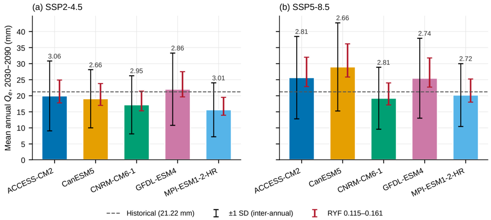
Across the behavioral range of the RYF (0.115–0.161), the mean annual Qe for 2030–2090 changes by −10.9% to +24.8% relative to the value at RYF = 0.129, for every GCM and scenario (Table 6; Supplementary Table S15). This range is a fixed proportion of Qe because Qe = RYF × Qp; it bounds the absolute magnitude of Qe but does not affect any percentage change, seasonal share, or trend significance reported above. For reference, the inter-annual standard deviation of Qe within each GCM is 2.66–3.06 times the RYF-induced half-width (Figure 6). This comparison describes the relative size of the two quantities and is not used as a measure of model robustness; uncertainty arising from the SCS-CN parameterization is assessed in Section 3.11.
Figure 6.
Mean annual effective runoff Qe during 2030–2090 for the five CMIP6 models under (a) SSP2–4.5 and (b) SSP5–8.5, calculated using RYF = 0.129. Colored bars represent the mean annual Qe; black error bars indicate ±1 interannual standard deviation, and red error bars show the range of Qe obtained using RYF values of 0.115–0.161 (−10.9% to +24.8% relative to RYF = 0.129). The dashed horizontal line indicates the historical mean (21.22 mm). Numbers above the bars represent the ratio of interannual standard deviation to the half-width of the RYF-induced range, given for reference only and not as a measure of model robustness.
3.9. Supporting Temperature Projections
The observed mean annual temperature of the ARB over 2001–2023 was 25.75 °C (ERA5-Land). The GCM historical simulations overestimated temperature by 1.06 °C for 2001–2014, with the largest warm bias during the NEM (+1.58 °C) and the smallest in the pre-monsoon months (+0.62 °C) (Supplementary Tables S5 and S16). The CMIP6 projections exhibited a persistent warming trend across the ARB during 2030–2090 under both future scenarios (Figure 7; Supplementary Table S16). The ensemble-mean annual temperature was 28.19 °C under SSP2–4.5 and 28.95 °C under SSP5–8.5, with inter-model standard deviations of 0.515 °C and 0.738 °C, respectively, corresponding to coefficients of variation of 1.83% and 2.55%.
Figure 7.
Projected temperature characteristics of the Amaravathi River Basin during 2030–2090: (a) annual ensemble-mean temperature under SSP2–4.5 and SSP5–8.5 with inter-model spread (±1 SD); and (b) seasonal ensemble-mean temperature under the two future scenarios.
The observed record showed a weak, non-significant warming trend over 2001–2023 (Sen’s slope = 0.013 °C yr−1, τ = 0.138, p = 0.369). In contrast, the projections showed statistically significant increasing temperature trends under both scenarios. Kendall’s τ was 0.796 for SSP2–4.5 and 0.907 for SSP5–8.5 (p < 0.001), while Sen’s slopes were 0.02592 °C yr−1 and 0.05864 °C yr−1, respectively. The corresponding 95% confidence intervals were 0.02304–0.02813 °C yr−1 for SSP2–4.5 and 0.05612–0.06100 °C yr−1 under SSP5–8.5. Based on Sen’s slope, temperature increased by 1.56 °C under SSP2–4.5 and 3.52 °C under SSP5–8.5 for 2030–2090. Relative to the GCM historical period (2001–2014), the ensemble mean for 2081–2090 was 1.93 °C warmer under SSP2–4.5 and 3.72 °C warmer under SSP5–8.5. Seasonally, summer/pre-monsoon was the warmest in both the observed record and the projections, with mean temperatures of 30.23 °C and 31.10 °C under SSP2–4.5 and SSP5–8.5, respectively, followed by the southwest monsoon, northeast monsoon, and winter seasons. Temperature was evaluated as a supporting climate indicator to characterize the broader future hydroclimatic conditions of the basin and was not used as a direct input to the SCS-CN runoff calculation.
3.10. Daily Characteristics of the Scenario Forcing
Over the period 2001–2014, the five GCM historical simulations reproduced CHIRPS annual precipitation within −16% to −4% (ensemble −10.8%), but it was distributed differently over the time period (Table 9; Figure 8). The simulations produced 20% fewer wet days (121.9 vs. 152.9 days yr−1; ranging from −34% to +8%) with higher intensity: the simple daily intensity was about 14% higher, the 95th wet-day percentile was 18% higher, and Rx5day 24% higher. The GCMs had fewer days in AMC-II and AMC-III (−27% and −14%) and 18% fewer days on which rainfall exceeded the initial abstraction of the basin CN (35.0 vs. 42.7 days yr−1), even though a larger share of their rainfall fell on those days (58% vs. 54%). CanESM5 differed from the other models, with more frequent but lighter rainy days (+8% wet days; −20% intensity), which explains its low historical Qp and therefore its large relative change against its own historical run. These differences in the timing and intensity of the daily rainfall, not only in the totals, explain why the GCM historical runs generate less Qp than the CHIRPS baseline, and they support evaluating the climate-change signal against each GCM’s own historical simulation. In the future, the number of runoff-producing days increased by 19% under SSP2–4.5 (four of five GCMs) and 41% under SSP5–8.5 (five of five), AMC-III days by 13% and 30%, and Rx1day by 5% and 15% (all five GCMs), consistent with the projected increase in Qe (Supplementary Table S12).
Table 9.
Daily precipitation characteristics of the NEX-GDDP-CMIP6 historical simulations compared with CHIRPS, 2001–2014 (basin-mean daily precipitation).
Figure 8.
Daily precipitation characteristics of the NEX-GDDP-CMIP6 historical simulations relative to CHIRPS for 2001–2014. (a) Quantile–quantile comparison of wet-day precipitation (≥1 mm); the dashed line indicates the 1:1 relationship, and the dotted vertical line indicates the initial abstraction (Ia) for the basin-wide CN-II. (b) Model-specific percentage biases in runoff-relevant daily precipitation indices relative to CHIRPS. Colors and symbols identify the five GCMs.
3.11. Influence of SCS-CN Parameterization on Future Runoff Projections
The CN-class model reproduced the relative changes of the distributed GEE model closely (r = 1.00 across GCMs, scenarios, and seasons; the median absolute difference 1.6 percentage points; same sign in 98% of cases). Across the seven configurations (Table 10; Figure 9), the annual, SWM, and NEM changes increased under both scenarios in every configuration, and only the small pre-monsoon change switched sign (−10.5% to +0.2% under SSP2–4.5 and −8.2% to +8.9% under SSP5–8.5; Supplementary Table S11). The AMC thresholds had the largest effect on magnitude, whereas the initial-abstraction ratio and the slope adjustment changed the annual ensemble change by no more than 2.2 and 0.4 percentage points, respectively. The projected direction of changes is thus robust to the SCS-CN parameterization, while its magnitude carries a parameter-related uncertainty that is smaller than the spread among GCMs (for example, SSP5–8.5 SWM: +63% to +120% across configurations vs. +1% to +331% across GCMs).
Table 10.
Ensemble change in potential runoff (Qp, %, 2030–2090 vs. each GCM’s own historical simulation) and model-implied precipitation elasticity εp (median GCM) under seven SCS-CN configurations.
Figure 9.
Ensemble changes in potential runoff Qp during 2030–2090 relative to each GCM’s own historical simulation under seven SCS-CN configurations: (a) SSP2–4.5 and (b) SSP5–8.5. Columns represent annual and seasonal changes (pre-monsoon, Southwest Monsoon [SWM], and Northeast Monsoon [NEM]), and rows represent the tested SCS-CN configurations. Values within cells indicate percentage changes, while the color scale represents the magnitude and direction of change.
4. Discussion
4.1. Rainfall Partitioning and the Conversion of Potential to Qe
The historical simulation provides the reference for interpreting the projected changes. The annual mean precipitation in the ARB was 1105.41 mm; SCS-CN potential runoff (Qp) was 164.50 mm (14.9% of precipitation) and, after applying the RYF of 0.129, Qe was 21.22 mm (1.92%). These are two sequential stages of the framework (Section 2.3 and Section 2.4) rather than a single rainfall–runoff coefficient.
The Qp/P ratio has to be interpreted as a catchment-specific outcome of the daily rainfall sequence and the spatial CN–AMC parameterization rather than against a universal runoff coefficient. Previously, studies related to SCS-CN have shown that estimated runoff is sensitive to the catchment’s heterogeneity, soil and land-cover characteristics, AMC, rainfall magnitude, and the way CN parameters are represented [6,9,10,77]. Studies from semi-arid and southern Indian catchments likewise report markedly different rainfall-to-runoff fractions, including an annual runoff coefficient of ~0.29 for the semi-arid Manesar Nala watershed and highly distinct SCS-CN runoff responses in South Indian basins [8,78,79]. These findings indicate that while the 14.9% Qp/P recorded for the ARB is physically reasonable, it represents a basin-specific characteristic rather than a benchmark value for semi-arid catchments.
The lower Qe relative to the Qp reflects a different hydrological scale rather than a contradictory calculation of rainfall–runoff. The potential runoff generated within the contributing area does not necessarily correlate with the effective runoff reaching the downstream outlet, particularly in basins that have storage and regulated flow systems. The SCS-CN formulation intends to estimate event-based direct runoff and does not explicitly resolve all downstream storage, routing, and flow-regulation processes [10]. In the ARB, this distinction is mainly relevant because supporting studies on the Amaravathi system describe the reservoir as a regulated irrigation system in which inflow, storage, and outflow vary with water demand, cropping patterns, water-use practices, and operating conditions [57]. A few independent hydrogeological studies have additionally provided insights that Amaravathi and its tributaries are strongly influenced by seasonal precipitation, with river flows limited to relatively short periods during the monsoon, while irrigation and domestic requirements are mostly dependent on groundwater where surface-water availability is limited [15]. These observations provide basin-specific context for distinguishing rainfall-generated potential runoff from effective runoff at the regional scale.
Accordingly, the RYF is an empirical bridge between potential runoff generation and effective regional runoff, rather than a process-specific loss term (Section 2.4). It does not individually quantify infiltration, recharge, channel transmission losses, local storage, abstraction, or reservoir operations. Thus, the effective runoff coefficient of 1.92% should not be interpreted as an indication that only 1.92% of the precipitation in the basin is used for runoff generation, nor should the difference between Qp and Qe be assigned to a single hydrological process.
4.2. Seasonal Redistribution of Precipitation and Qe
The future projections indicate that the principal seasonal change in the ARB is a redistribution of precipitation and effective runoff across the annual cycle, rather than a uniform change across all seasons. The SWM (Southwest Monsoon; June–September) becomes increasingly important to the basin’s effective runoff response, whereas the summer and NEM (Northeast Monsoon; October–December) exhibit a weaker and more scenario-dependent response.
The two baselines lead to the same conclusion for the SWM but not for the other seasons. The SWM increase is found against both baselines, in all five GCMs, under SSP5–8.5, without CanESM5, and under every SCS-CN configuration tested, whereas the pre-monsoon and NEM decreases found against CHIRPS largely disappear, or reverse, against the models’ own historical simulations and are attributed mainly to model bias rather than to projected change (Section 3.3 and Section 3.10).
As a result, the SWM share of annual Qe rises from 28.8% historically to more than 41% under both scenarios (Section 3.3; Table 4), so future change is expressed through the seasonal distribution of runoff as well as its annual magnitude.
The projected SWM response is consistent with broader CMIP6 literature for Indian regions. Multi-model CMIP6 assessments generally project an increase in June–September rainfall under future warming, with a stronger response under high-emission pathways. Katzenberger et al. [1] used multiple CMIP6 models and reported a robust increase in Indian monsoon rainfall with warming, while Norgate et al. [80] similarly used multiple CMIP6 models across Indian precipitation regions and found increasing future summer-monsoon precipitation together with substantial differences among models and regions. The agreement between these studies and the ARB projections provides a direction of the seasonal response, rather than magnitude, as the present study uses a different model ensemble for the spatial domain and rainfall–runoff framework. These studies associate the increase with a thermodynamic increase in atmospheric moisture together with the changes in circulation and moisture transport [1,80]; the present study does not diagnose these mechanisms for the ARB.
The comparison becomes more relevant at the regional scale. A recent CMIP6–VIC assessment of the southern Western Ghats and Western Coastal Plains states a combined wetter Indian summer monsoon condition, together with increasing runoff under SSP2–4.5 and SSP5–8.5 [13]. This provides a particularly relevant analog for the ARB because the broad climatic setting and seasonal structure are comparable. The hydrological model is independent of the SCS-CN approach used here. The consistent shift toward a wetter monsoon and drier pre-monsoon across multiple modeling frameworks is consistent with the seasonal redistribution found in the ARB being a climate-driven signal rather than an artifact of the runoff model. However, the magnitude of the projected runoff changes cannot be compared directly between the studies because of differing catchment domains, hydrological formulation, climate-model ensembles, and differing runoff definitions.
The NEM response is weaker, and its sign depends on the baseline: NEM Qe decreases relative to CHIRPS but increases relative to the models’ own historical runs (Section 3.3). This is compatible with the complex and uncertain NEM rainfall regime over southern peninsular India, for which CMIP5 and CMIP6 models show high interannual variability, low predictability, and difficulty in reproducing ENSO-, Indian Ocean Dipole-, sea-surface temperature, and circulation-related relationships [81]. A large model-to-model spread in projected changes, which differ among individual NEM months, has been reported [82]. The present study does not attribute these differences to a particular atmospheric teleconnection.
The runoff response adds an important hydrological dimension to these climatic changes. The historical NEM contribution to effective runoff is larger than that of the SWM, with mean seasonal Qe values of 12.44 and 6.11 mm, respectively. Under the future scenarios, however, the SWM contribution rises to more than 41% of annual Qe, while the relative contribution of the NEM declines. The significance of this result therefore does not imply that one season becomes wetter and the other drier; rather, the seasonal concentration of effective runoff itself changes. As the runoff calculation uses daily precipitation together with antecedent five-day rainfall to determine the moisture conditions, timing, and sequencing of rainfall can influence the amount of precipitation which converts to potential runoff. Previous SCS-CN studies have demonstrated the importance of antecedent moisture and rainfall characteristics in determining runoff response [6,77]. The stronger SWM runoff response in the ARB should therefore be interpreted as a combined outcome of the projected seasonal precipitation change and its transformation through the daily SCS-CN framework, rather than as a direct proportional response to the seasonal rainfall anomaly.
4.3. Non-Proportional and Spatially Heterogeneous Future Runoff Response
The projected effective runoff does not respond proportionally to the change in annual precipitation. The model-implied precipitation elasticity of effective runoff was about 1.9 in the historical baseline and under both scenarios (1.72–2.09 across the models; Table 8), within the range commonly reported for catchments worldwide [63,64]; as explained in Section 2.6, it reflects the threshold non-linearity of the SCS-CN method rather than an independently observed property of the basin, and it varied from 1.48 to 2.24 across SCS-CN configurations (Section 3.11). However, annual precipitation changes alone do not fully explain the projected ensemble-mean changes. Under SSP2–4.5, an elasticity of about 1.9 applied to a 2.15% decrease in precipitation would imply a decrease in Qe of roughly 4%, whereas the projected decrease was 11.52%. This indicates that changes in the seasonal and daily distribution of rainfall, discussed below, also contribute to the projected runoff response.
This non-proportional response is consistent with the inherent non-linear formulation of the SCS-CN method. In this framework, runoff is governed by the interaction between rainfall and the available abstraction represented by the curve number, rather than by a constant rainfall–runoff coefficient. Consequently, incremental changes seen in the precipitation can produce disproportionately larger or smaller changes in runoff depending on the hydrological state of the catchment [10]. The influence of AMC also further strengthens this non-linear behavior because wetter initial conditions reduce the remaining storage capacities and increase the runoff generation by subsequent rainfall [40,83]. Hence, the differences between the precipitation and effective-runoff responses obtained for these scenarios are physically consistent with a rainfall–runoff system in which the same increment of rainfall does not need to generate the same runoff increment.
Rainfall intensity and temporal distribution also matter: concentrated rainfall can produce more rainfall excess than the same amount spread over a longer interval [84], and because AMC is assigned from five-day antecedent rainfall, changes in the sequencing of wet and dry days can modify the runoff response even when seasonal or annual totals change little (Section 3.10).
The projected response is also spatially heterogeneous across the ARB; Qe increased over about 70% (SSP2–4.5) and 81% (SSP5–8.5) of the basin area, but as the forcing is resolved at 0.25°, these fractions describe the pattern at the scale of about 12 GCM cells modulated by the CN distribution, rather than at 500 m. Under SSP2–4.5, the basin-scale ensemble mean decreases by 11.52% relative to the historical reference. This contrast is apparently seen because the magnitude of negative changes over parts of the basin is sufficient to outweigh more widespread but comparatively small positive changes. Under SSP5–8.5, the widespread increase is consistent with the positive basin-average response. The result demonstrates that the basin-average statistic represents an aggregation of spatially heterogeneous responses and should not be interpreted as an indicator of the direction of change at every location.
This spatial heterogeneity is expected in a distributed SCS-CN framework because CN and runoff generation vary with soil properties, LULC, soil-water storage capacity, and antecedent wetness [10]. Applications of GIS-based SCS-CN in South Indian watersheds show similar variation in land use and soil characteristics, followed by substantial spatial differences in runoff response [78]. The broader Western Ghats also support this interpretation, as the catchment characteristics and hydrological response vary across physiographically differentiated areas [79]. Therefore, the spatial pattern obtained for the ARB should be viewed as an emergent response of heterogeneous landscape properties interacting with spatially varying future precipitation.
The spatial results are also consistent with documented hydroclimatic heterogeneity within the ARB’s districts. The rainfall analysis for the Dindigul district of the ARB reports substantial spatial and seasonal rainfall variability, including the differing contribution of the NEM and SWM [85]. This district-scale (rather than basin-wide) evidence helps in interpreting why a uniform scenario-scale precipitation change does not necessarily generate a spatially uniform runoff response across the ARB. Evidence from the wider Cauvery system likewise indicates strong spatial contrasts in runoff potential associated with differences in LULC and soil characteristics and further supports the relevance of spatially distributed runoff assessment in this regional setting [86].
4.4. Temporal Trends, Model Variability, and Hydroclimatic Warming
Under SSP2–4.5, the ensemble-mean effective runoff of 18.78 mm remains low when compared to the historical mean of 21.22 mm. However, the projected ensemble-mean annual series shows a statistically significant increasing trend of 0.084 mm yr−1 (p = 0.0065) and a strong trend of 0.236 mm yr−1 (p < 0.001) under SSP5–8.5, with a mean of 23.90 mm. At the individual model level, however, significant Qe trends were found in only one of the five GCMs under SSP2–4.5 and four of five under SSP5–8.5 (Table 5), indicating that the ensemble-mean trends reflect a subset of models. These results indicate that comparison of future and historical means reflects a change in average state, whereas the Mann–Kendall trend defines the temporal evolution within the future period. The two metrics therefore provide complementary information and should not be interpreted as an equivalent measure of change. The upper end of the projected runoff distribution also differs between the scenarios, as, under SSP2–4.5, the maximum annual effective runoff reaches 28.62 mm, with a Qe95 of 25.75 mm. SSP5–8.5 produces a maximum of 38.73 mm and a Qe95 of 34.38 mm. Thus, the stronger forcing scenario produces larger upper-end runoff values with the selected ensemble. These ARB results are consistent with CMIP6 assessments over India, showing that precipitation changes and precipitation extremes generally become stronger under higher-emission scenarios, although substantial regional and model-to-model differences remain [1,2,80,87].
The five-GCM ensemble highlights inter-model variability in both rainfall and effective runoff. The coefficient of variation of annual precipitation increases from 16.80% (SSP2–4.5) to 21.49% (SSP5–8.5), whereas that of effective runoff also increases from 13.19% under SSP2–4.5 to 17.09% under SSP5–8.5. Only two models showed rainfall increases relative to the historical mean under either scenario, while effective runoff increases in one out of five models under SSP2–4.5 and three of five models under SSP5–8.5. Few of these model-specific differences were statistically significant (Table 7; Supplementary Table S2).
The role of CanESM5, a high-sensitivity model whose inclusion can overstate changes [35,37], is assessed in Section 3.6: it drives the SSP5–8.5 increase in annual precipitation relative to CHIRPS, whereas the SWM increase and the SSP5–8.5 increase in Qe relative to the models’ own historical runs are reproduced by the other four models.
CMIP6 studies show that inter-model differences arise from differences in the representation of precipitation processes, circulation, and associated climate responses, so the model spread should be retained when the projections are analyzed [88,89,90]. The temperature projections also act as a complementary indicator to understand the changing hydroclimatic environment of the basin. Relative to their own historical simulations, the models project end-century (2081–2090) warming of 1.93 °C under SSP2–4.5 and 3.72 °C under SSP5–8.5, with strong positive trends (Section 3.9; Supplementary Table S16), which is consistent with the scenario-dependent warming reported across CMIP6 projections for South Asia [2].
Temperature is not an explicit input to the runoff calculation used in this study, and temperature-dependent processes such as evapotranspiration are not dynamically represented. Hydrological assessments have shown that evapotranspiration and associated land-surface processes can modify runoff and water-resource responses to climate change, even though precipitation changes remain the primary control on runoff [90,91]. The basin currently has a semi-arid to dry sub-humid climate (aridity index, 0.47–0.64, Section 2.1), with a mean annual PET of about 1726 mm. Based on the temperature dependence of the Hargreaves formulation [92], in which PET scales with (T + 17.8), the projected end-century warming would increase PET by 4% under SSP2–4.5 and 9% under SSP5–8.5, assuming unchanged radiation and diurnal temperature range. Higher evaporative demand would tend to reduce soil moisture and hence runoff generation. This effect would be strongest during the warm pre-monsoon season, so the projected increases in effective runoff, especially under SSP5–8.5, may represent upper estimates.
Three sources of uncertainty were assessed separately. First, inter-model (GCM) uncertainty is largest: under SSP5–8.5, for example, the change in SWM Qe relative to own historical runs ranges from +0.6% to +340% across the five GCMs. Second, varying the SCS-CN parameterization across seven configurations changes the magnitude of the projected changes but not their direction for the annual, SWM, and NEM totals (Section 3.11). Third, uncertainty in the RYF affects only the absolute Qe, by −10.9% to +24.8% (Section 3.8). These tests bound the uncertainty within the adopted framework but are not a complete uncertainty decomposition: the structural differences between SCS-CN and process-based models and the changes in landuse, storage, and regulation are not represented. Sensitivity studies of SCS-CN parameters demonstrate that runoff estimates can respond to parameter choices and can differentiate between the parameter sensitivity and broader sources of modeling variability [77].
4.5. Implications, Limitations, and Scope of Interpretation
The projected changes in effective runoff lie primarily in the timing and spatial distribution of runoff generation, rather than in the change in annual runoff alone. Across nearly 22 Indian river basins, the annual and monsoon-season rainfall trends were not always consistent, indicating that water-resource planning should consider proper seasonal timing and variability in addition to the annual totals [14]. Because the SWM increase is the most consistent result (Section 4.2), future water-resource implications in the ARB should be evaluated on a seasonal basis: additional wet-season runoff does not automatically imply improved water availability in the lower-runoff seasons.
Similarly, studies related to the Western Ghats catchments have combined climate and land-use changes and produced contrasting streamflow conditions across the seasons to support agricultural water availability and cropping periods [93]. A CMIP6–SWAT assessment of the neighboring Ponnaiyar River Basin in Tamil Nadu similarly projects substantial period-dependent changes in annual surface runoff, reinforcing that seasonal and multidecadal timing govern water-resource outcomes in the basin [11]. Bhave et al. [94] used an integrated climate and socioeconomic water-resource framework for the portion of the Cauvery basin in Karnataka. The study showed that future water-supply reliability depends on the interaction between climate-driven water availability and changing water demand. The adaptation pathways usually involve demand management and can improve robustness under uncertainty. For the ARB, the seasonal redistribution of Qe therefore points to the need to assess whether the existing seasonal storages and allocation mechanisms can adequately accommodate changes in the timing and magnitude of the runoff. However, this cannot be determined solely from the present framework; it requires a water-balance and reservoir-operation model with reservoir capacity, operating rules, and downstream demand. Interventions that increase local water retention or availability can modify downstream flows.
The interpretation of future water availability is further constrained by the limited surface-water observations across the ARB. The RYF is constrained by streamflow observations from the nested Kodavanar sub-basin, for which CWC discharge data are available only for 2021–2023 (Section 2.4). The present framework cannot resolve how much water is retained within the storage systems, diverted, abstracted for irrigation, or ultimately expressed as downstream discharge, because it does not dynamically represent the groundwater, baseflow, channel routing, or reservoir operations. Hence, Qe should not be interpreted directly as future reservoir inflows or downstream discharge.
Independent groundwater evidence provides an important context for this surface-water limitation. Senthilkumar et al. [15] reported nearly 1475.11 million m3 of annual replenishable groundwater resources for the Amaravathi aquifer system and found that 74 of 107 groundwater assessment units were categorized as over-exploited or critical, with groundwater withdrawal exceeding the annual groundwater recharge in these units [15]. The study further reports that flow in Amaravathi, Noyil, and associated tributaries is limited to a maximum of 10–15 days during the monsoon period. This highlights the importance of groundwater for meeting irrigation and domestic requirements where surface-water availability is limited. These findings are consistent with groundwater-resource assessments reported by the Central Ground Water Board (CGWB), which state a gross groundwater draft of nearly 1640.35 million m3 and an average stage of groundwater development of 111% for the assessed area [95]. The groundwater evidence should not be interpreted as quantities derived from the present Qe estimates; rather, it provides an independent indication of groundwater dependence and groundwater-resource stress in the Amaravathi system. The surface-water projections alone are not sufficient to characterize basin-wide water-resource stress. A spatially distributed streamflow-gauging network combined with systematic groundwater-level monitoring would therefore be necessary to quantify the interactions among surface-water availability, groundwater dependence, recharge, and water demand in the ARB.
In the upper Cauvery catchment, Wable et al. [16] identified that agricultural water-management interventions harvest nearly 140–160 million cubic meters of surface runoff upstream, reducing inflow into the Krishnaraja Sagar reservoir by 2–6% directly. This illustrates the upstream and downstream trade-offs at the basin scale. Reservoirs and abstraction can also modify natural flow regimes in the basin, as also reported by Ekka et al. [58], who found that changes in median flows, minimum flows, and low-flow pulses were associated with the reservoir construction and water abstractions. For the ARB, the appropriate implication is not about the particular structures implemented, such as check dams, tanks, or additional reservoirs, but that seasonal storage and runoff management interventions should be evaluated using basin-scale water-balance and upstream–downstream analyses before the site-specific decisions are implemented.
The stronger response under SSP5–8.5 is consistent with CMIP6 studies across South Asia and India [1,2] and supports testing existing storage, drainage, and runoff management systems across several plausible climates rather than a single scenario; SSP5–8.5 results should be considered as an upper-range scenario within this study and not as a deterministic prediction of future flood occurrence. Consistent with this, the indicative frequency suggests that both deficient and excess rainfall years may become more frequent than in the historical period (about 9% of years each), with excess years reaching about 25–36% of years and deficient years about 13–20%, depending on the scenario (Supplementary Table S7); given the wide spread among the GCMs, these frequencies indicate a tendency toward greater hydroclimatic variability rather than predictions of specific drought or flood years.
Because basin-average changes can conceal contrasting local responses (Section 4.3), as also reported for the Western Ghats and Cauvery regions [93,96], the spatial Qe maps are best used as a screening layer, at the 0.25° resolution of the forcing, to identify areas that warrant more detailed assessment (Table 11).
Table 11.
ARB findings, hydrological interpretation, implications for further assessment, and supporting evidence.
The transferability of the findings therefore operates primarily at the level of hydrological and management principles rather than numerical projections. Evidence from studies mentioned in Table 11 provides a broader context for interpreting the ARB results, whereas the magnitude and spatial distribution of the projected effective-runoff response remain specific to the ARB.
There are six limitations of the study that define the scope of these implications. First, 2022 landuse/landcover was held constant throughout the future simulation. This isolates the climate-forcing component of the projected runoff change but does not represent the future urban expansion, agricultural conversion, or vegetative change, although combined climate and land-use changes can produce different hydrological responses [93]. Second, and importantly, the RYF rests on a single gauged sub-basin and three NEM seasons (eight monthly values); cross-validation was modest (out-of-sample NSE of 0.67), volume errors for individual withheld seasons ranged from −52.5% to +84.8% (Supplementary Table S3), the basin-outlet check (Supplementary Table S14) supports its transfer to the whole basin at the annual scale only, and the assumption that it remains constant across seasons and into the future could not be tested with the available record. Absolute Qe values should therefore be read as indicative, whereas relative changes do not depend on the RYF. Third, as discussed above, the framework does not represent groundwater, baseflow, channel routing, or reservoir operations, which have altered flows elsewhere in the Cauvery [16,58]. Fourth, temperature was analyzed only as a hydroclimatic indicator; evapotranspiration and vegetation responses, which can materially influence projected water-resource outcomes, are not represented, so the results are a framework-driven assessment rather than a complete water balance. Fifth, five selected GCMs and two SSP scenarios characterized inter-model variability within this ensemble only; multi-model ensembles reduce, but do not eliminate, the systematic bias in runoff projection [97], so the model agreement statistics and coefficient of variation describe the selected models, not probabilities of occurrence. Sixth, the SCS-CN method has no explicit soil-moisture accounting, its parameters (λ and CN) are applied uniformly across varied terrain so that slope effects are represented only approximately (Section 2.3), and the NEX-GDDP-CMIP6 forcing has fewer wet days and more intense rainfall than CHIRPS (Section 3.10), which is why only findings that agree under both baselines are treated as robust.
Overall, these findings support a climate-informed but process-aware approach to Amaravathi water-resource planning. The principal implication is not a specific infrastructure prescription, but the need to evaluate whether existing systems remain robust to changes in seasonal runoff timing, spatial distribution, interannual variability, and upper-end runoff conditions. Studies from the Cauvery basin indicate that such evaluation is most informative when climate projections are taken into consideration with agricultural demand, storage, reservoir operations, and downstream requirements. The Amaravathi projections therefore provide a basin-specific hydroclimatic evidence layer for subsequent integrated assessment. Beyond the specific projections for the ARB, the broader contribution of this study lies in demonstrating a data-constrained approach for future runoff assessment in a basin. A sufficiently long and continuous basin- and sub-basin-outlet discharge record is not available for direct calibration of the distributed future hydrological model. The available nested gauged catchments were therefore used to derive an empirical regional yield factor that provides a practical bridge between distributed SCS-CN potential runoff and basin-scale effective runoff. This framework distinguishes Qp from Qe and separately quantifies inter-model variability, baseline-related, SCS-CN parameter, and RYF-related uncertainty. By integrating seasonal redistribution, spatial heterogeneity, temporal trends, runoff extremes, model variability, and parameter sensitivity, the study characterizes multiple dimensions of future hydrological change within a single basin-specific framework. This approach provides a potentially transferable basis for future runoff assessment in other data-constrained basins, subject to the availability of an appropriate nested gauged catchment and independent evaluation of the regionalization assumptions.
5. Conclusions
This study developed a data-constrained, spatially distributed CMIP6–SCS-CN framework to assess future effective runoff in the ARB, using an empirically derived regional yield factor from a nested gauged catchment to translate distributed potential runoff into a gauge-constrained index of runoff yield. Relative to the historical baseline (2001–2023) of 1105.41 mm precipitation and 21.22 mm effective runoff, SSP2–4.5 projected a net decline (−2.15% precipitation, −11.52% effective runoff), while SSP5–8.5 projected an increase in both (+9.67% and +12.64%), but neither Qe change was statistically significant (95% confidence intervals include zero). Relative to the models’ own historical simulations, Qe increased by 13.60% and 44.62%, with all five GCMs increasing under SSP5–8.5. The SSP5–8.5 increase in annual precipitation relative to CHIRPS depended on CanESM5, whereas the increase in Qe relative to the models’ own runs did not. Ensemble-mean Qe showed significant increasing trends within 2030–2090 under both scenarios, driven by one of five GCMs under SSP2–4.5 and four of five under SSP5–8.5. The model-implied precipitation elasticity of about 1.9 reflected the threshold non-linearity of the SCS-CN method rather than an independent property of the basin.
The most robust result is the seasonal redistribution of runoff yield. SWM Qe increased by 26–72% relative to CHIRPS and by 33–81% relative to the models’ own historical runs, and the SWM share of annual Qe rose from 28.8% to 41.0–44.0%. This increase was found against both baselines, without CanESM5, and under all seven SCS-CN configurations tested. The pre-monsoon and NEM decreases relative to CHIRPS largely reflected the GCM dry bias and fewer runoff-producing days in the GCM forcing. Spatial patterns of change are resolved only at the 0.25° scale of the forcing. The results rest on a single RYF calibrated in one sub-basin over three NEM seasons: its cross-validated skill is modest (out-of-sample NSE = 0.67), single-season volume errors are large (−52.5% to +84.8%), its transfer to the whole basin is supported only at the annual scale by the outlet check, and its transferability to other seasons and into the future remains untested, so absolute Qe values are indicative while relative changes are independent of the RYF. The results are further bounded by a five-model unweighted ensemble and by a framework that does not represent evapotranspiration, groundwater exchange, or reservoir operation; the results therefore characterize the climate-driven change in the runoff yield, not a full water balance.
Future research in the ARB should prioritize continuous basin-outlet (including the individual sub-basins) discharge monitoring and systematic groundwater observations. These datasets are essential for calibrating and validating distributed hydrological models. Coupling the framework with dynamic landuse, evapotranspiration, weighted GCM ensembles, and reservoir operation would allow the seasonal shift identified here to be assessed in terms of storage and allocation. In the interim, this study provides a seasonally and spatially resolved, uncertainty-bounded baseline of projected runoff-yield change for a basin without continuous monitoring.
Supplementary Materials
The following supporting information can be downloaded at: https://www.mdpi.com/article/10.3390/hydrology13110301/s1, Figure S1: Observed and simulated monthly runoff depth at Lakshmananpatti (NEM 2021–2023): calibration with RYF = 0.129 and leave-one-season-out predictions. Dashed line: 1:1; Figure S2: Basin-outlet check of the regional yield factor at Nallamaranpatty (whole ARB, 2001–2015; Table S14); Table S1: Mann–Kendall trend statistics of annual precipitation (P) and effective runoff (Qe), with autocorrelation-corrected tests; Table S2: Model-specific changes in mean annual precipitation (P) and effective runoff (Qe), 2030–2090, relative to the CHIRPS baseline (2001–2023) and to each GCM’s own historical simulation (2001–2014); Table S3: Derivation, calibration range and leave-one-season-out (LOSO) cross-validation of the regional yield factor (RYF); Table S4: Historical GCM precipitation bias relative to CHIRPS (%); Table S5: Historical GCM mean temperature (°C) and bias relative to ERA5-Land; Table S6: Non-parametric model-implied precipitation elasticity of effective runoff (εP); Table S7: Frequency of deficient and excess rainfall years; Table S8: Change in potential runoff (Qp, %) relative to each GCM’s own historical simulation (2001–2014); Table S9: Comparison of inference approaches for the annual ensemble-mean change relative to the CHIRPS baseline; Table S10: Projected change in annual precipitation (P) and Qe relative to the CHIRPS baseline for three 23-year future windows equal in length to the baseline; Table S11: Change in potential runoff (Qp, %, 2030–2090 vs. each GCM’s own historical simulation) for all seven SCS-CN configurations, seasons and scenarios; Table S12: Projected change in daily precipitation indices (2030–2090 vs. each GCM’s own historical simulation, 2001–2014); Table S13: Complete SCS-CN parameterization used in Google Earth Engine; Table S14: Basin-outlet check of the regional yield factor: annual observed runoff at Nallamaranpatty (CWC) compared with simulated potential (Qp) and effective runoff (Qe) for the whole ARB, 2001–2015; Table S15: Sensitivity of mean annual effective runoff (Qe, 2030–2090) to uncertainty in the regional yield factor (behavioral range 0.115–0.161; adopted value 0.129), compared with inter-annual variability, for the five CMIP6 models under SSP2–4.5 and SSP5–8.5. The inter-annual standard deviation (SD) and the ratio SD/half-width are given for reference only, to compare the size of the two quantities; they are not a measure of model robustness; Table S16: Historical and projected annual and seasonal temperature characteristics of the Amaravathi River Basin.
Author Contributions
Conceptualization, R.P.K. and S.G.; methodology, R.P.K. and S.G.; software, R.P.K.; validation, R.P.K., S.G. and C.S.; formal analysis, R.P.K.; investigation, R.P.K.; resources, S.G. and C.S.; data curation, R.P.K.; writing—original draft preparation, R.P.K.; writing—review and editing, S.G. and C.S.; visualization, R.P.K.; supervision, S.G. and C.S.; project administration, S.G. All authors have read and agreed to the published version of the manuscript.
Funding
This research received no external funding.
Data Availability Statement
Data will be made available upon request.
Acknowledgments
The authors express their gratitude to Karunya Institute of Technology and Sciences for providing laboratory facilities and essential support throughout the study.
Conflicts of Interest
The authors declare no conflicts of interest.
References
- Katzenberger, A.; Schewe, J.; Pongratz, J.; Levermann, A. Robust increase of Indian monsoon rainfall and its variability under future warming in CMIP6 models. Earth Syst. Dyn. 2021, 12, 367–386. [Google Scholar] [CrossRef] [Scilit]
- Almazroui, M.; Saeed, S.; Saeed, F.; Islam, M.N.; Ismail, M. Projections of precipitation and temperature over the South Asian countries in CMIP6. Earth Syst. Environ. 2020, 4, 297–320. [Google Scholar] [CrossRef] [Scilit]
- Salunke, P.; Keshri, N.P.; Mishra, S.K.; Dash, S.K. Future projections of seasonal temperature and precipitation for India. Front. Clim. 2023, 5, 1069994. [Google Scholar] [CrossRef] [Scilit]
- Huang, Q.; Qin, G.; Zhang, Y.; Tang, Q.; Liu, C.; Xia, J.; Chiew, F.H.S.; Post, D.A. Using remote sensing data-based hydrological model calibrations for predicting runoff in ungauged or poorly gauged catchments. Water Resour. Res. 2020, 56, e2020WR028205. [Google Scholar] [CrossRef] [Scilit]
- Singh, R.; Mishra, V.; Narasimhan, B.; Ghosh, S.; Sharma, A.; Dutta, S.; Mujumdar, P.P. Hydrological modeling in India. Proc. Indian Natl. Sci. Acad. 2020, 86, 479–494. [Google Scholar] [CrossRef] [Scilit]
- Mishra, S.K.; Jain, M.K.; Pandey, R.P.; Singh, V.P. Catchment area-based evaluation of the AMC-dependent SCS-CN-based rainfall–runoff models. Hydrol. Process. 2005, 19, 2701–2718. [Google Scholar] [CrossRef] [Scilit]
- Mishra, S.K.; Singh, V.P. A relook at NEH-4 curve number data and antecedent moisture condition criteria. Hydrol. Process. 2006, 20, 2755–2768. [Google Scholar] [CrossRef] [Scilit]
- Rawat, K.S.; Mishra, A.K.; Ahmad, N. Surface runoff estimation over heterogeneous foothills of Aravalli mountain using medium resolution remote sensing rainfall data with soil conservation system-curve number method: A case of semi-arid ungauged Manesar Nala watershed. Water Environ. J. 2017, 31, 262–276. [Google Scholar] [CrossRef] [Scilit]
- Soulis, K.X.; Valiantzas, J.D. SCS-CN parameter determination using rainfall-runoff data in heterogeneous watersheds—The two-CN system approach. Hydrol. Earth Syst. Sci. 2012, 16, 1001–1015. [Google Scholar] [CrossRef] [Scilit]
- Bartlett, M.S.; Parolari, A.J.; McDonnell, J.J.; Porporato, A. Beyond the SCS-CN method: A theoretical framework for spatially lumped rainfall-runoff response. Water Resour. Res. 2016, 52, 4608–4627. [Google Scholar] [CrossRef] [Scilit]
- Balu, A.; Ramasamy, S.; Sankar, G. Assessment of climate change impact on hydrological components of Ponnaiyar river basin, Tamil Nadu using CMIP6 models. J. Water Clim. Change 2023, 14, 730–747. [Google Scholar] [CrossRef] [Scilit]
- Visweshwaran, R.; Ramsankaran, R.A.A.J.; Eldho, T.I.; Jha, M.K. Hydrological impact assessment of future climate change on a complex river basin of Western Ghats, India. Water 2022, 14, 3571. [Google Scholar] [CrossRef] [Scilit]
- Thomas, J.; Rohith, A.N.; Sebastian, D.E.; Nizar, S.; Jainet, P.J.; Vema, V.K.; Sudheer, K.P. Climate warming modifies hydrological responses in the southern Western Ghats and the western coastal plains (India): Insights from CMIP6-VIC simulations. J. Environ. Manag. 2025, 381, 125252. [Google Scholar] [CrossRef] [Scilit]
- Kumar, V.; Jain, S.K. Trends in rainfall amount and number of rainy days in river basins of India (1951–2004). Hydrol. Res. 2011, 42, 290–306. [Google Scholar] [CrossRef] [Scilit]
- Senthilkumar, M.; Gnanasundar, D.; Arumugam, R. Identifying groundwater recharge zones using remote sensing & GIS techniques in Amaravathi aquifer system, southern India. Sustain. Environ. Res. 2019, 29, 15. [Google Scholar] [CrossRef] [Scilit]
- Wable, P.S.; Garg, K.K.; Nune, R.; Venkataradha, A.; Anantha, K.H.; Srinivasan, V.; Ragab, R.; Rowan, J.; Keller, V.; Majumdar, P.; et al. Impact of agricultural water management interventions on upstream–downstream trade-offs in the upper Cauvery catchment, southern India: A modelling study. Irrig. Drain. 2022, 71, 472–494. [Google Scholar] [CrossRef] [Scilit]
- Thrasher, B.; Wang, W.; Michaelis, A.; Melton, F.; Lee, T.; Nemani, R. NASA Global Daily Downscaled Projections, CMIP6. Sci. Data 2022, 9, 262. [Google Scholar] [CrossRef] [Scilit] [PubMed]
- Calizaya, F.; Cuentas, O.; Mejía, A.; Calizaya, E.; Cuentas, M.; Pozo, M.; Caira, C.; Huacani, W. GIS-based SCS-CN modeling of surface runoff under CMIP6 climate change scenarios and land cover dynamics in the high-Andean Ilave River Basin, Peru. Model. Earth Syst. Environ. 2026, 12, 216. [Google Scholar] [CrossRef] [Scilit]
- Muñoz-Sabater, J.; Dutra, E.; Agustí-Panareda, A.; Albergel, C.; Arduini, G.; Balsamo, G.; Boussetta, S.; Choulga, M.; Harrigan, S.; Hersbach, H.; et al. ERA5-Land: A state-of-the-art global reanalysis dataset for land applications. Earth Syst. Sci. Data 2021, 13, 4349–4383. [Google Scholar] [CrossRef] [Scilit]
- National Water Development Agency. A Case Study of Cauvery River Basin in South India; Government of India: New Delhi, India, 2020. Available online: https://www.nwda.gov.in (accessed on 22 October 2026).
- Kalaivanan, K.; Gurugnanam, B.; Suresh, M.; Kom, K.P.; Kumaravel, S. Geoelectrical resistivity investigation for hydrogeology conditions and groundwater potential zone mapping of Kodavanar sub-basin, southern India. Sustain. Water Resour. Manag. 2019, 5, 1281–1301. [Google Scholar] [CrossRef] [Scilit]
- Abatzoglou, J.T.; Dobrowski, S.Z.; Parks, S.A.; Hegewisch, K.C. TerraClimate, a high-resolution global dataset of monthly climate and climatic water balance from 1958–2015. Sci. Data 2018, 5, 170191. [Google Scholar] [CrossRef] [Scilit] [PubMed]
- United Nations Environment Programme. World Atlas of Desertification, 2nd ed.; Edward Arnold: London, UK, 1997. [Google Scholar]
- Funk, C.; Peterson, P.; Landsfeld, M.; Pedreros, D.; Verdin, J.; Shukla, S.; Husak, G.; Rowland, J.; Harrison, L.; Hoell, A.; et al. The climate hazards infrared precipitation with stations—A new environmental record for monitoring extremes. Sci. Data 2015, 2, 150066. [Google Scholar] [CrossRef] [Scilit] [PubMed]
- Peterson, P.; Funk, C.; Landsfeld, M.; Husak, G.; Pedreros, D.; Verdin, J.; Rowland, J.; Shukla, S.; McNally, A.; Michaelsen, J.; et al. The Climate Hazards Group InfraRed Precipitation with Stations (CHIRPS) dataset: Quasi-global precipitation estimates for drought monitoring and trend analysis. In Proceedings of the AGU Fall Meeting, San Francisco, CA, USA, 15–19 December 2014. [Google Scholar]
- Divya, P.; Shetty, A. Evaluation of CHIRPS satellite rainfall datasets over Kerala, India. In Trends in Civil Engineering and Challenges for Sustainability; Narasimhan, M.C., George, V., Kumar, U., Kumar, G., Eds.; Springer: Singapore, 2021; pp. 655–664. [Google Scholar] [CrossRef] [Scilit]
- Geleta, C.D.; Deressa, T.A. Evaluation of Climate Hazards Group InfraRed Precipitation Station (CHIRPS) satellite-based rainfall estimates over Finchaa and Neshe Watersheds, Ethiopia. Eng. Rep. 2021, 3, e12338. [Google Scholar] [CrossRef] [Scilit]
- O’Neill, B.C.; Tebaldi, C.; van Vuuren, D.P.; Eyring, V.; Friedlingstein, P.; Hurtt, G.; Knutti, R.; Kriegler, E.; Lamarque, J.-F.; Lowe, J.; et al. The scenario model intercomparison project (ScenarioMIP) for CMIP6. Geosci. Model Dev. 2016, 9, 3461–3482. [Google Scholar] [CrossRef] [Scilit]
- Riahi, K.; van Vuuren, D.P.; Kriegler, E.; Edmonds, J.; O’Neill, B.C.; Fujimori, S.; Bauer, N.; Calvin, K.; Dellink, R.; Fricko, O.; et al. The shared socioeconomic pathways and their energy, land use, and greenhouse gas emissions implications: An overview. Glob. Environ. Change 2017, 42, 153–168. [Google Scholar] [CrossRef] [Scilit]
- IPCC. Summary for Policymakers. In Climate Change 2021: The Physical Science Basis. Contribution of Working Group I to the Sixth Assessment Report of the Intergovernmental Panel on Climate Change; Masson-Delmotte, V., Zhai, P., Pirani, A., Connors, S.L., Péan, C., Berger, S., Caud, N., Chen, Y., Goldfarb, L., Gomis, M.I., et al., Eds.; Cambridge University Press: Cambridge, UK, 2021; pp. 3–32. [Google Scholar] [CrossRef] [Scilit]
- Hausfather, Z.; Peters, G.P. Emissions—The ‘business as usual’ story is misleading. Nature 2020, 577, 618–620. [Google Scholar] [CrossRef] [Scilit] [PubMed]
- Divyadharshini, S.; Geethalakshmi, V.; Bhuvaneshwari, K.; Dheebakaran, G.A.; Karthikeyan, R.; Thirukumaran, K.; Karthick, V.; Mohan Kumar, S. Future projections of rainfall for Tamil Nadu from Coupled Model Intercomparison Project-6 (CMIP6). Int. J. Environ. Clim. Change 2023, 13, 461–471. [Google Scholar] [CrossRef] [Scilit]
- Patel, G.; Das, S.; Das, R. Identification of best CMIP6 global climate model for rainfall by ensemble implementation of MCDM methods and statistical inference. Water Resour. Manag. 2023, 37, 5147–5170. [Google Scholar] [CrossRef] [Scilit]
- Meehl, G.A.; Senior, C.A.; Eyring, V.; Flato, G.; Lamarque, J.-F.; Stouffer, R.J.; Taylor, K.E.; Schlund, M. Context for interpreting equilibrium climate sensitivity and transient climate response from the CMIP6 Earth system models. Sci. Adv. 2020, 6, eaba1981. [Google Scholar] [CrossRef] [Scilit]
- Swart, N.C.; Cole, J.N.S.; Kharin, V.V.; Lazare, M.; Scinocca, J.F.; Gillett, N.P.; Anstey, J.; Arora, V.; Christian, J.R.; Hanna, S.; et al. The Canadian Earth System Model version 5 (CanESM5.0.3). Geosci. Model Dev. 2019, 12, 4823–4873. [Google Scholar] [CrossRef] [Scilit]
- Forster, P.; Storelvmo, T.; Armour, K.; Collins, W.; Dufresne, J.-L.; Frame, D.; Lunt, D.J.; Mauritsen, T.; Palmer, M.D.; Watanabe, M.; et al. The Earth’s energy budget, climate feedbacks, and climate sensitivity. In Climate Change 2021: The Physical Science Basis. Contribution of Working Group I to the Sixth Assessment Report of the Intergovernmental Panel on Climate Change; Masson-Delmotte, V., Zhai, P., Pirani, A., Connors, S.L., Péan, C., Berger, S., Caud, N., Chen, Y., Goldfarb, L., Gomis, M.I., et al., Eds.; Cambridge University Press: Cambridge, UK, 2021; pp. 923–1054. [Google Scholar] [CrossRef] [Scilit]
- Hausfather, Z.; Marvel, K.; Schmidt, G.A.; Nielsen-Gammon, J.W.; Zelinka, M. Climate simulations: Recognize the ‘hot model’ problem. Nature 2022, 605, 26–29. [Google Scholar] [CrossRef] [Scilit] [PubMed]
- Manikpuri, S.; Tripathi, M.P. Estimation of surface runoff potential using SCS-CN method integrated with GIS approach in Nawagarh watershed of Seonath Sub-Basin, Chhattisgarh. J. Soil Water Conserv. 2026, 24, 111–119. [Google Scholar] [CrossRef] [Scilit]
- Adam, E.O.; Abd Elbasit, M.A.M.; Solomon, T.; Ahmed, F. Integration of satellite rainfall data and curve number method for runoff estimation under semi-arid wadi system. Int. Arch. Photogramm. Remote Sens. Spat. Inf. Sci. 2017, XLII-3/W2, 1–7. [Google Scholar] [CrossRef] [Scilit]
- Gundalia, M.; Dholakia, M. Impact of monthly curve number and five-day antecedent rainfall-runoff data set on performance of SCS-CN method for Ozat watershed in India—A case study. Int. J. Adv. Eng. Res. Dev. 2014, 1, 125–133. [Google Scholar] [CrossRef] [Scilit]
- Jacobs, J.M.; Myers, D.A.; Whitfield, B.M. Improved rainfall/runoff estimates using remotely sensed soil moisture. J. Am. Water Resour. Assoc. 2003, 39, 313–324. [Google Scholar] [CrossRef] [Scilit]
- USDA-SCS. National Engineering Handbook, Section 4: Hydrology; Soil Conservation Service, U.S. Department of Agriculture: Washington, DC, USA, 1972.
- Hawkins, R.H.; Hjelmfelt, A.T.; Zevenbergen, A.W. Runoff probability, storm depth, and curve numbers. J. Irrig. Drain. Eng. 1985, 111, 330–340. [Google Scholar] [CrossRef] [Scilit]
- Ponce, V.M.; Hawkins, R.H. Runoff curve number: Has it reached maturity? J. Hydrol. Eng. 1996, 1, 11–19. [Google Scholar] [CrossRef] [Scilit]
- Garen, D.C.; Moore, D.S. Curve number hydrology in water quality modeling: Uses, abuses, and future directions. J. Am. Water Resour. Assoc. 2005, 41, 377–388. [Google Scholar] [CrossRef] [Scilit]
- Neitsch, S.L.; Arnold, J.G.; Kiniry, J.R.; Williams, J.R. Soil and Water Assessment Tool Theoretical Documentation, Version 2009; Technical Report No. 406; Texas Water Resources Institute: College Station, TX, USA, 2011. [Google Scholar]
- Mishra, S.K.; Singh, V.P. Soil Conservation Service Curve Number (SCS-CN) Methodology; Kluwer Academic Publishers: Dordrecht, The Netherlands, 2003. [Google Scholar] [CrossRef] [Scilit]
- Michel, C.; Andréassian, V.; Perrin, C. Soil Conservation Service Curve Number method: How to mend a wrong soil moisture accounting procedure? Water Resour. Res. 2005, 41, W02011. [Google Scholar] [CrossRef] [Scilit]
- Hawkins, R.H.; Jiang, R.; Woodward, D.E.; Hjelmfelt, A.T.; Van Mullem, J.A. Runoff curve number method: Examination of the initial abstraction ratio. In Proceedings of the Second Federal Interagency Hydrologic Modeling Conference, Las Vegas, NV, USA, 28 July–1 August 2002. [Google Scholar]
- Woodward, D.E.; Hawkins, R.H.; Jiang, R.; Hjelmfelt, A.T.; Van Mullem, J.A.; Quan, Q.D. Runoff curve number method: Examination of the initial abstraction ratio. In Proceedings of the World Water & Environmental Resources Congress 2003; ASCE: Reston, VA, USA, 2003; pp. 1–10. [Google Scholar] [CrossRef] [Scilit]
- Sharpley, A.N.; Williams, J.R. (Eds.) EPIC—Erosion/Productivity Impact Calculator: 1. Model Documentation; USDA Technical Bulletin No. 1768; U.S. Department of Agriculture: Washington, DC, USA, 1990.
- Huang, M.; Gallichand, J.; Wang, Z.; Goulet, M. A modification to the Soil Conservation Service curve number method for steep slopes in the Loess Plateau of China. Hydrol. Process. 2006, 20, 579–589. [Google Scholar] [CrossRef] [Scilit]
- Taye, M.T.; Zimale, F.A.; Woldesenbet, T.A.; Kebede, M.G.; Amare, S.D.; Tegegne, G.; Mekonnen, K.; Haile, A.T. Priority research topics to improve streamflow data availability in data-scarce countries: The case for Ethiopia. Hydrology 2023, 10, 220. [Google Scholar] [CrossRef] [Scilit]
- Moriasi, D.N.; Arnold, J.G.; Van Liew, M.W.; Bingner, R.L.; Harmel, R.D.; Veith, T.L. Model evaluation guidelines for systematic quantification of accuracy in watershed simulations. Trans. ASABE 2007, 50, 885–900. [Google Scholar] [CrossRef] [Scilit]
- Knoben, W.J.M.; Freer, J.E.; Woods, R.A. Technical note: Inherent benchmark or not? Comparing Nash–Sutcliffe and Kling–Gupta efficiency scores. Hydrol. Earth Syst. Sci. 2019, 23, 4323–4331. [Google Scholar] [CrossRef] [Scilit]
- Yamazaki, D.; Ikeshima, D.; Sosa, J.; Bates, P.D.; Allen, G.H.; Pavelsky, T.M. MERIT Hydro: A high-resolution global hydrography map based on latest topography dataset. Water Resour. Res. 2019, 55, 5053–5073. [Google Scholar] [CrossRef] [Scilit]
- Moorthi, P.V.P.; Singh, A.P.; Agnivesh, P. Regulation of water resources systems using fuzzy logic: A case study of Amaravathi dam. Appl. Water Sci. 2018, 8, 132. [Google Scholar] [CrossRef] [Scilit]
- Ekka, A.; Keshav, S.; Pande, S.; van der Zaag, P.; Jiang, Y. Dam-induced hydrological alterations in the upper Cauvery river basin, India. J. Hydrol. Reg. Stud. 2022, 44, 101231. [Google Scholar] [CrossRef] [Scilit]
- Maraun, D. Bias correcting climate change simulations—A critical review. Curr. Clim. Change Rep. 2016, 2, 211–220. [Google Scholar] [CrossRef] [Scilit]
- Cannon, A.J.; Sobie, S.R.; Murdock, T.Q. Bias correction of GCM precipitation by quantile mapping: How well do methods preserve changes in quantiles and extremes? J. Clim. 2015, 28, 6938–6959. [Google Scholar] [CrossRef] [Scilit]
- Gusain, A.; Ghosh, S.; Karmakar, S. Added value of CMIP6 over CMIP5 models in simulating Indian summer monsoon rainfall. Atmos. Res. 2020, 232, 104680. [Google Scholar] [CrossRef] [Scilit]
- Meena, M. Rainfall statistical trend and variability detection using Mann-Kendall test, Sen’s slope and coefficient of variance—A case study of Udaipur district (1957–2016). Appl. Ecol. Environ. Sci. 2020, 8, 34–37. [Google Scholar] [CrossRef]
- Sankarasubramanian, A.; Vogel, R.M.; Limbrunner, J.F. Climate elasticity of streamflow in the United States. Water Resour. Res. 2001, 37, 1771–1781. [Google Scholar] [CrossRef] [Scilit]
- Chiew, F.H.S. Estimation of rainfall elasticity of streamflow in Australia. Hydrol. Sci. J. 2006, 51, 613–625. [Google Scholar] [CrossRef] [Scilit]
- Mann, H.B. Nonparametric tests against trend. Econometrica 1945, 13, 245–259. [Google Scholar] [CrossRef] [Scilit]
- Kendall, M.G. Rank Correlation Methods, 4th ed.; Charles Griffin: London, UK, 1975. [Google Scholar]
- Sen, P.K. Estimates of the regression coefficient based on Kendall’s tau. J. Am. Stat. Assoc. 1968, 63, 1379–1389. [Google Scholar] [CrossRef]
- Yadav, R.; Tripathi, S.K.; Pranuthi, G.; Dubey, S.K. Trend analysis by Mann-Kendall test for precipitation and temperature for thirteen districts of Uttarakhand. J. Agrometeorol. 2014, 16, 164–171. [Google Scholar] [CrossRef] [Scilit]
- Kamal, N.; Pachauri, S. Mann-Kendall and Sen’s slope estimators for precipitation trend analysis in North-Eastern States of India. Int. J. Comput. Appl. 2019, 177, 7–16. [Google Scholar] [CrossRef] [Scilit]
- Partal, T.; Kahya, E. Trend analysis in Turkish precipitation data. Hydrol. Process. 2006, 20, 2011–2026. [Google Scholar] [CrossRef] [Scilit]
- Hamed, K.H.; Rao, A.R. A modified Mann-Kendall trend test for autocorrelated data. J. Hydrol. 1998, 204, 182–196. [Google Scholar] [CrossRef] [Scilit]
- Yue, S.; Pilon, P.; Phinney, B.; Cavadias, G. The influence of autocorrelation on the ability to detect trend in hydrological series. Hydrol. Process. 2002, 16, 1807–1829. [Google Scholar] [CrossRef] [Scilit]
- Gilbert, R.O. Statistical Methods for Environmental Pollution Monitoring; Van Nostrand Reinhold: New York, NY, USA, 1987. [Google Scholar]
- Maurya, S.; Srivastava, P.K.; Zhuo, L.; Yaduvanshi, A.; Mall, R.K. Future climate change impact on the streamflow of Mahi River Basin under different general circulation model scenarios. Water Resour. Manag. 2023, 37, 2675–2696. [Google Scholar] [CrossRef] [Scilit]
- Mann, H.B.; Whitney, D.R. On a test of whether one of two random variables is stochastically larger than the other. Ann. Math. Stat. 1947, 18, 50–60. [Google Scholar] [CrossRef] [Scilit]
- Efron, B.; Tibshirani, R.J. An Introduction to the Bootstrap; Chapman & Hall: New York, NY, USA, 1993. [Google Scholar]
- Hosseini, S.M.; Mahjouri, N. Sensitivity and fuzzy uncertainty analyses in the determination of SCS-CN parameters from rainfall-runoff data. Hydrol. Sci. J. 2018, 63, 457–473. [Google Scholar] [CrossRef] [Scilit]
- Satheeshkumar, S.; Venkateswaran, S.; Kannan, R. Rainfall–runoff estimation using SCS–CN and GIS approach in the Pappiredipatti watershed of the Vaniyar sub basin, South India. Model. Earth Syst. Environ. 2017, 3, 24. [Google Scholar] [CrossRef] [Scilit]
- Viji, R.; Prasanna, P.R.; Ilangovan, R. Modified SCS-CN and Green-Ampt methods in surface runoff modelling for the Kundahpallam watershed, Nilgiris, Western Ghats, India. Aquat. Procedia 2015, 4, 677–684. [Google Scholar] [CrossRef] [Scilit]
- Norgate, M.; Tiwari, P.R.; Das, S.; Kumar, D. On the present and future changes in Indian summer monsoon precipitation characteristics under different SSP scenarios from CMIP6 models. Clim. Dyn. 2024, 62, 10445–10464. [Google Scholar] [CrossRef] [Scilit]
- Sreekala, P.P.; Babu, C.A.; Rao, S.V.B. On the simulation of northeast monsoon rainfall over southern peninsular India in CMIP5 and CMIP6 models. Theor. Appl. Climatol. 2022, 150, 969–986. [Google Scholar] [CrossRef] [Scilit]
- Tiwari, R.; Mishra, A.K.; Rai, S.; Pandey, L.K. Evaluation and projection of northeast monsoon precipitation over India under higher warming scenario: A multimodel assessment of CMIP6. Theor. Appl. Climatol. 2022, 151, 859–870. [Google Scholar] [CrossRef] [Scilit]
- Ghosh, S.; Guchhait, S.K. Geomorphic threshold and SCS-CN-based runoff and sediment yield modelling in the gullies of Dwarka–Brahmani Interfluve, West Bengal, India. In Gully Erosion Studies from India and Surrounding Regions; Shit, P.K., Pourghasemi, H.R., Bhunia, G.S., Eds.; Springer: Cham, Switzerland, 2019; pp. 45–68. [Google Scholar] [CrossRef] [Scilit]
- Mertens, J.; Raes, D.; Feyen, J. Incorporating rainfall intensity into daily rainfall records for simulating runoff and infiltration into soil profiles. Hydrol. Process. 2002, 16, 731–739. [Google Scholar] [CrossRef] [Scilit]
- Thangamani, S.; Raviraj, A. Rainfall variability and trend detection in Dindigul district of Amaravathi Basin. Curr. World Environ. 2016, 11, 567–576. [Google Scholar] [CrossRef] [Scilit]
- Karthik, K.C.; Prashanta, M.; Ravikumar, D.; Devagiri, G.M.; Murali, K.V. Runoff dynamics and soil erosion assessment using a SWAT model at Upper Cauvery River Basin. Int. J. Environ. Clim. Change 2024, 14, 292–307. [Google Scholar] [CrossRef] [Scilit]
- Varghese, S.J.; Pentakota, S.; Thadivalasa, P.; Podapati, G.; Ashok, K. Changes in physical characteristics of extreme rainfall events during the Indian summer monsoon based on downscaled and bias-corrected CMIP6 models. Sci. Rep. 2025, 15, 3679. [Google Scholar] [CrossRef] [Scilit]
- Guilbert, M.; Terray, P.; Mignot, J. Intermodel spread of historical Indian monsoon rainfall change in CMIP6: The role of the tropical Pacific mean state. J. Clim. 2023, 36, 3937–3953. [Google Scholar] [CrossRef] [Scilit]
- Long, S.-M.; Li, G. Model uncertainty in the projected Indian summer monsoon precipitation change under low-emission scenarios. Atmosphere 2021, 12, 248. [Google Scholar] [CrossRef] [Scilit]
- Zhao, T.; Dai, A. CMIP6 model-projected hydroclimatic and drought changes and their causes in the twenty-first century. J. Clim. 2022, 35, 897–921. [Google Scholar] [CrossRef] [Scilit]
- Peiris, T.A.; Döll, P. Improving the quantification of climate change hazards by hydrological models: A simple ensemble approach for considering the uncertain effect of vegetation response to climate change on potential evapotranspiration. Hydrol. Earth Syst. Sci. 2023, 27, 3663–3686. [Google Scholar] [CrossRef] [Scilit]
- Hargreaves, G.H.; Samani, Z.A. Reference crop evapotranspiration from temperature. Appl. Eng. Agric. 1985, 1, 96–99. [Google Scholar] [CrossRef] [Scilit]
- Sharannya, T.M.; Venkatesh, K.; Mudbhatkal, A.; Dineshkumar, M.; Mahesha, A. Effects of land use and climate change on water scarcity in rivers of the Western Ghats of India. Environ. Monit. Assess. 2021, 193, 820. [Google Scholar] [CrossRef] [Scilit]
- Bhave, A.G.; Conway, D.; Dessai, S.; Stainforth, D.A. Water resource planning under future climate and socioeconomic uncertainty in the Cauvery River Basin in Karnataka, India. Water Resour. Res. 2018, 54, 708–728. [Google Scholar] [CrossRef] [Scilit]
- Central Ground Water Board. Aquifer Mapping and Ground Water Management: Amaravathi Basin, Tamil Nadu; Government of India: New Delhi, India, 2022. Available online: https://cgwb.gov.in/sites/default/files/2022-11/amravathi-i.pdf (accessed on 22 October 2026).
- Sreelash, K.; Mathew, M.M.; Nisha, N.; Arulbalaji, P.; Bindu, A.G.; Sharma, R.K. Changes in the hydrological characteristics of Cauvery river draining the eastern side of southern Western Ghats, India. Int. J. River Basin Manag. 2020, 18, 153–166. [Google Scholar] [CrossRef] [Scilit]
- Hou, Y.; Guo, H.; Yang, Y.; Liu, W. Global evaluation of runoff simulation from climate, hydrological and land surface models. Water Resour. Res. 2023, 59, e2021WR031817. [Google Scholar] [CrossRef] [Scilit]
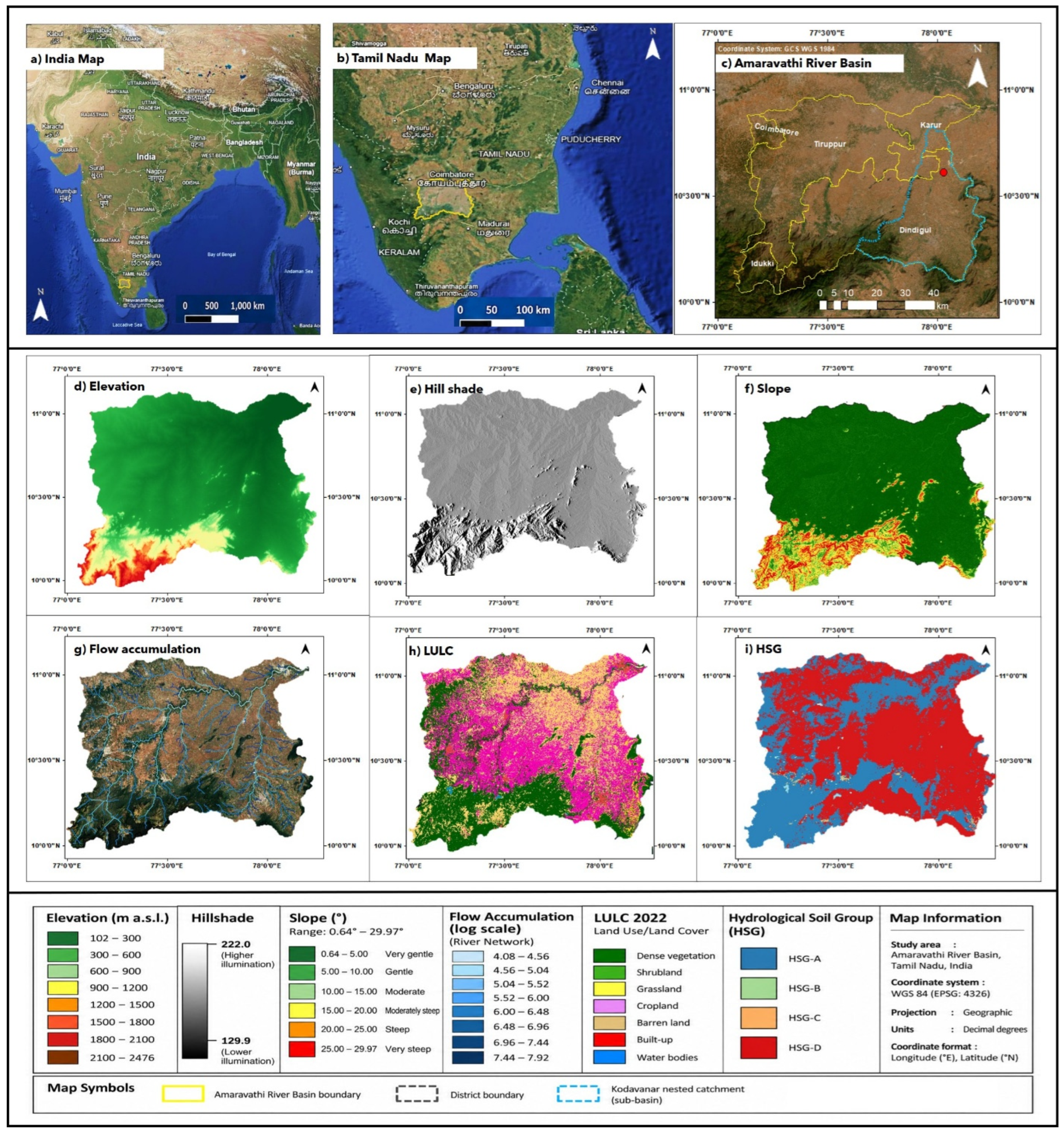
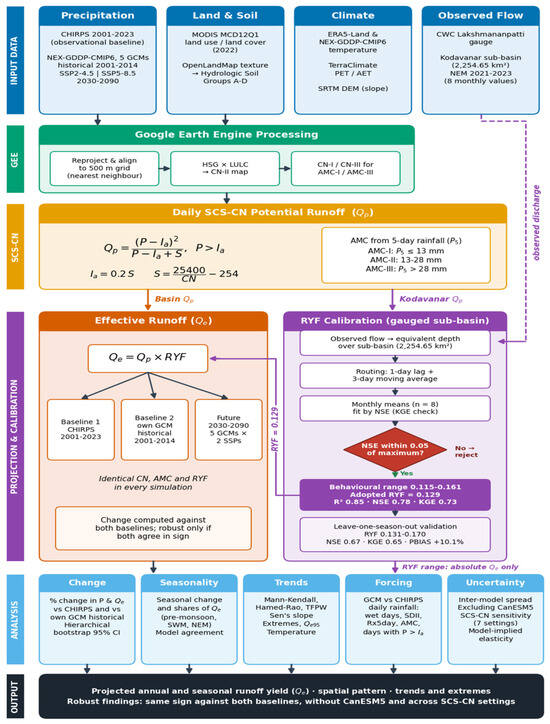
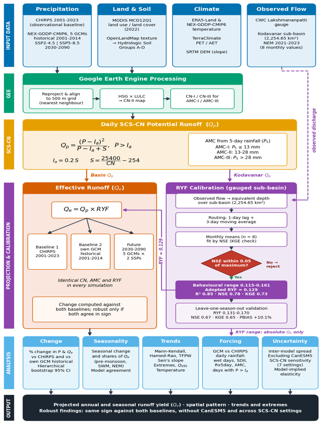
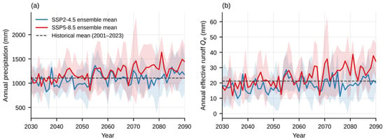
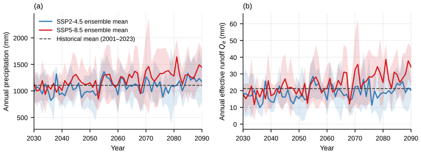
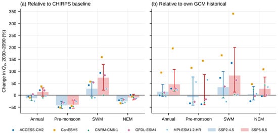
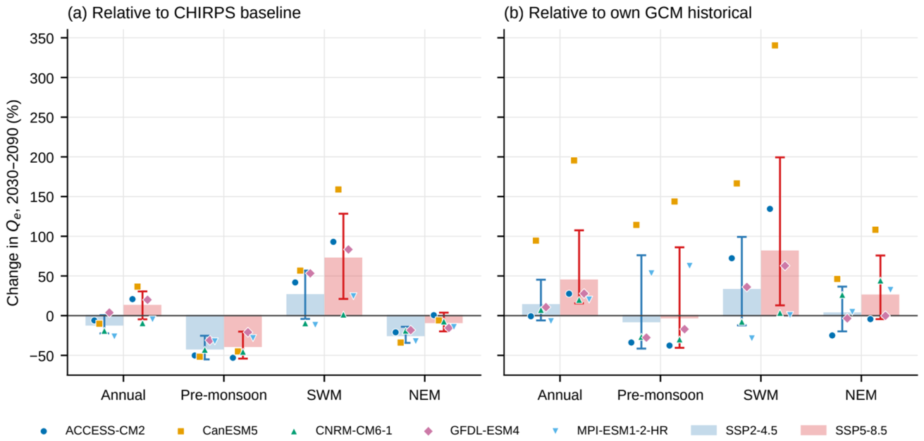
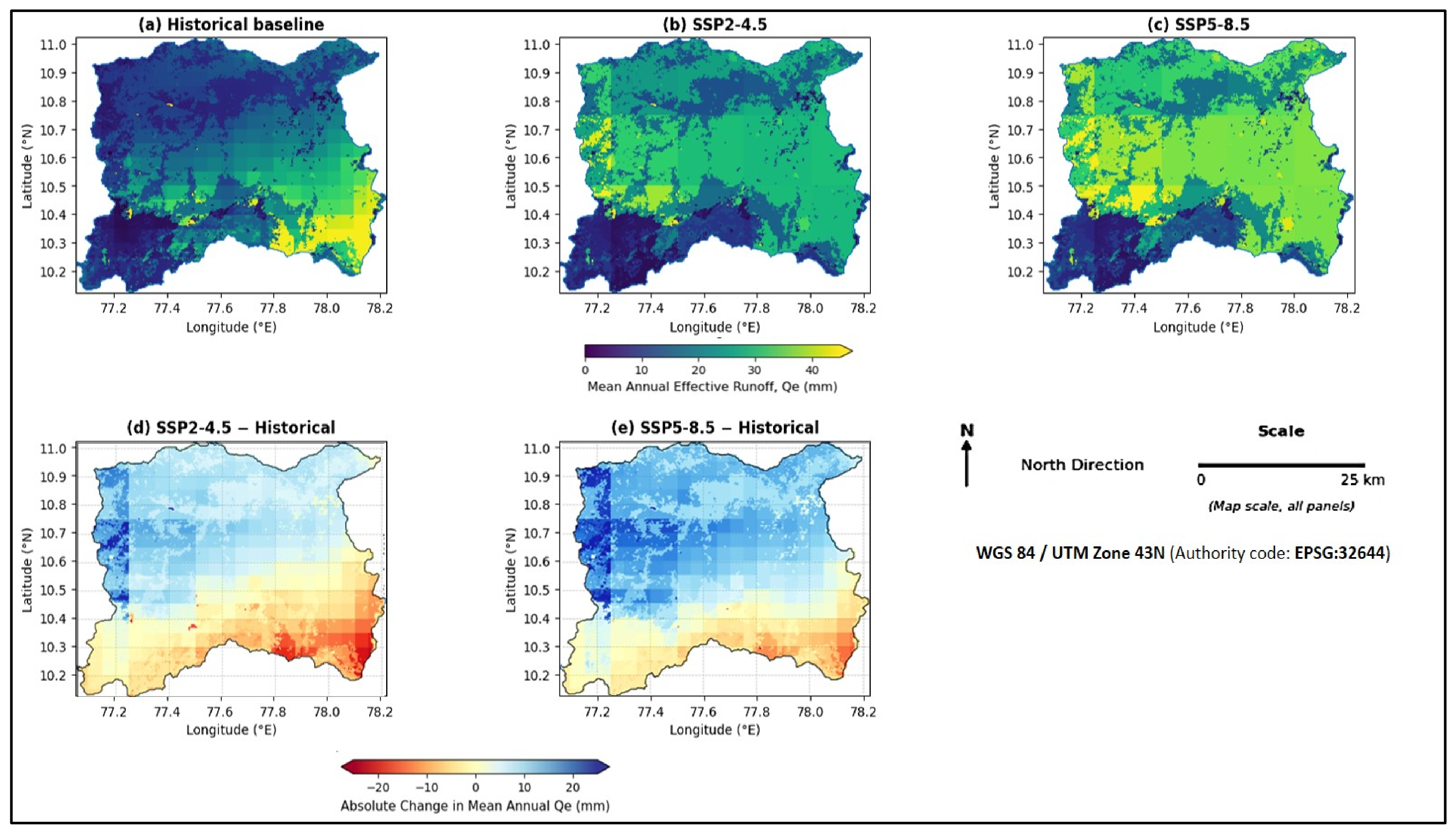
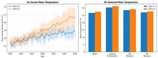
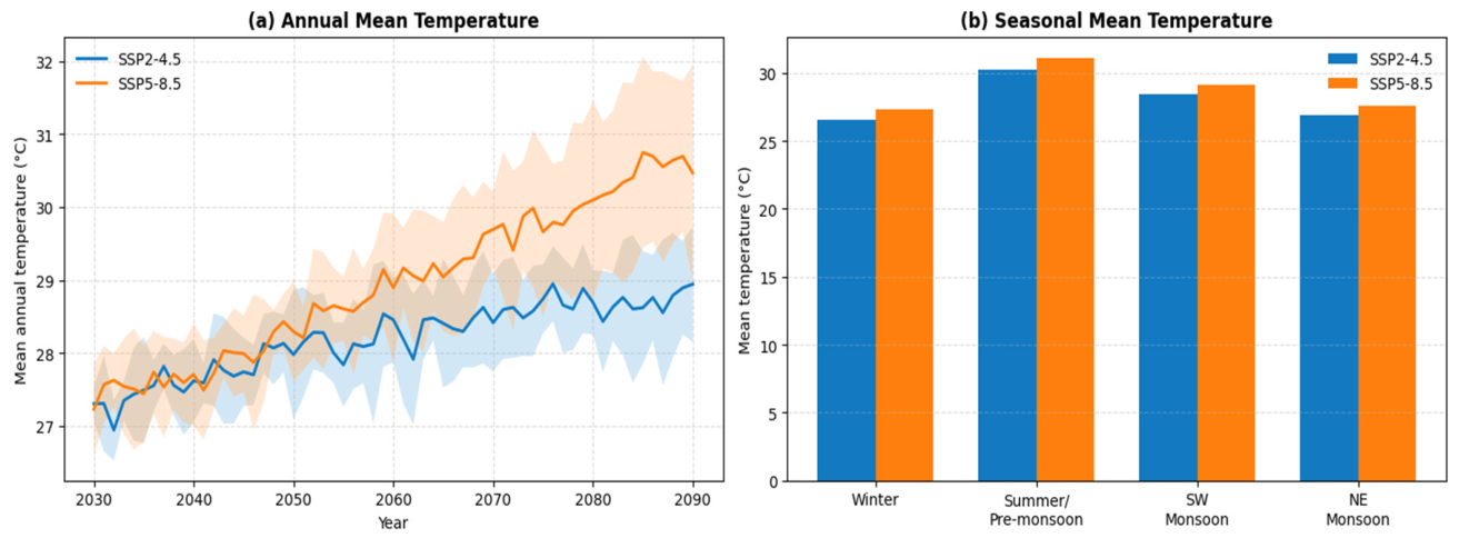
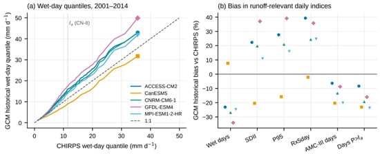
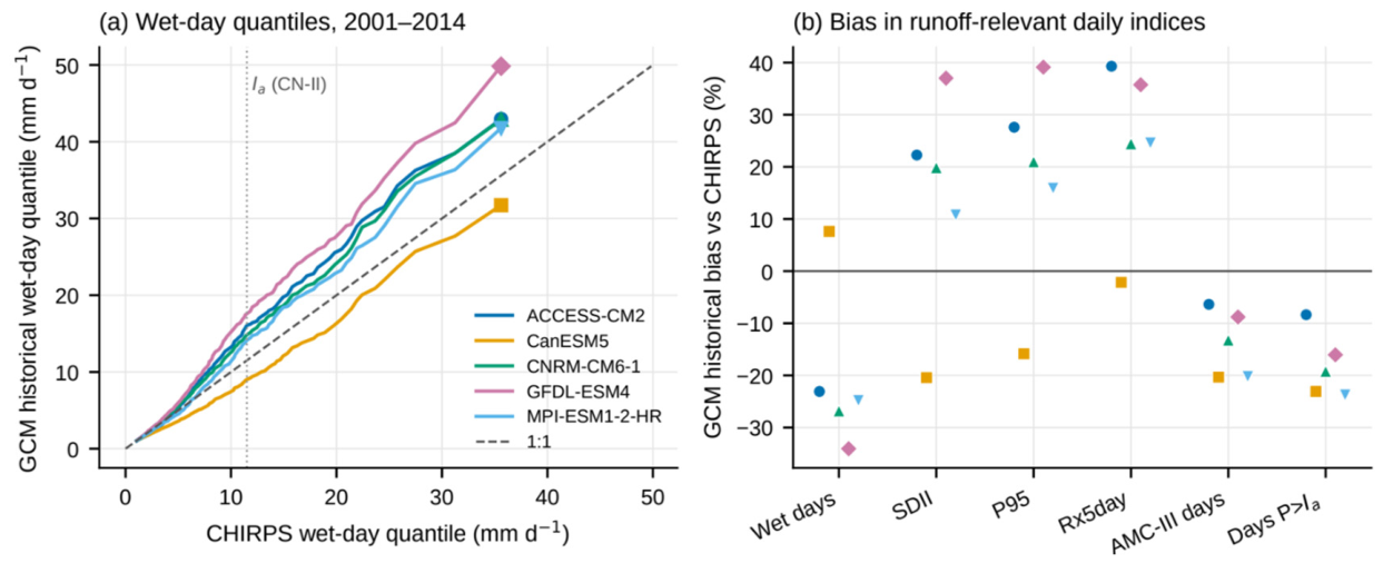
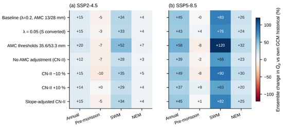
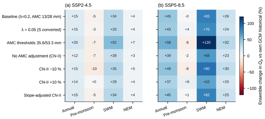

Disclaimer/Publisher’s Note: The statements, opinions and data contained in all publications are solely those of the individual author(s) and contributor(s) and not of MDPI and/or the editor(s). MDPI and/or the editor(s) disclaim responsibility for any injury to people or property resulting from any ideas, methods, instructions or products referred to in the content. |
© 2026 by the authors. Licensee MDPI, Basel, Switzerland. This article is an open access article distributed under the terms and conditions of the Creative Commons Attribution (CC BY) license.