


Abstract
Continuous meteorological records are essential for hydrological studies, yet station records often contain gaps. This study benchmarks 31 statistical, geostatistical, machine-learning and deep-learning methods for reconstructing isolated missing values and short gaps in daily precipitation and air temperature records in the Myjava River Basin, western Slovakia (1981–2020; 19 precipitation and 3 air temperature stations retained after excluding two stations dominated by multi-year interruptions). After diagnosing the structure and mechanism of missing data, all methods were evaluated by 20 repetitions of Monte Carlo cross-validation, in which every method was refitted, using error metrics with uncertainty estimates and significance tests, together with wet-day occurrence, dry and wet spells, extremes and physical plausibility. For air temperature, multiple imputation by chained equations (MICE) and several of the best-performing machine-learning methods were significantly more accurate than distance-based methods (RMSE 0.97–1.00 versus 1.38–1.41 °C), which do not account for systematic differences between stations at different elevations. For precipitation, the distance-based normal ratio, inverse-distance k-nearest-neighbour and inverse distance weighting methods were practically as accurate as MICE (RMSE 1.87–1.89 versus 1.85 mm; differences below 2%) while preserving dry days and producing no negative values. Method complexity therefore mattered for air temperature but not for precipitation. The propagation of reconstruction errors into simulated runoff was not assessed and is the subject of ongoing research.
1. Introduction
Hydrological modelling relies on temporally consistent meteorological forcing, yet long observational records commonly contain gaps and discontinuities. Precipitation and air temperature are primary controls of runoff generation, snow and soil moisture dynamics, evapotranspiration, and catchment water balance; therefore, their continuity and measurement consistency are essential for reliable hydroclimatic assessment and hydrological simulation [1,2,3,4,5]. Despite improvements in monitoring systems, meteorological time series still suffer from missing observations caused by instrument malfunction, station relocation or closure, acquisition errors, and operational limitations [4,6,7]. If such gaps are not handled appropriately, they introduce uncertainty into climatological analyses, distort hydroclimatic interpretation, and propagate errors into hydrological simulations [8,9].
The problem is particularly acute for precipitation and, to a lesser extent, air temperature because missing values alter not only sample size but also the statistical structure, spatial structure and temporal dependence of the series. Daily precipitation is highly intermittent, spatially heterogeneous, and often nonlinearly related across neighbouring stations, which makes it especially sensitive to reconstruction errors that can smooth variability, attenuate extremes, and distort event timing and volume [7,10]. Air temperature is generally more spatially coherent, but its gaps can still affect snowmelt estimation, evapotranspiration calculations, and energy-balance-related hydrological processes. Missing data may occur as short sporadic gaps or as long discontinuities associated with station closure, and these different forms of missingness require different reconstruction strategies [6], consistent with international guidance emphasizing the importance of continuity and quality control in meteorological station networks [11]. Previous studies have shown that incomplete meteorological datasets can introduce systematic bias and reduce inferential reliability in hydroclimatic and hydrological applications [5]. Maintaining continuous and physically representative meteorological records is therefore a prerequisite for robust long-term analysis.
A broad range of gap-filling methods has been developed to reconstruct incomplete meteorological series. Conventional approaches such as arithmetic averaging, normal ratio estimation, regression models, and inverse distance weighting (IDW) remain widely used because they are computationally efficient, transparent, and easy to implement [6,12,13]. Even relatively simple spatially weighted methods may improve precipitation estimates when neighbouring information is used effectively [12]. More advanced geostatistical techniques, including kriging-based interpolation, explicitly represent spatial correlation structures and may therefore better exploit inter-station dependence [7]. Copula-based approaches further extend this logic by modelling dependence structure and uncertainty more flexibly, particularly for precipitation [10]. Multi-station regression frameworks and optimized combinations of linear and nonlinear components have also shown robust performance in precipitation reconstruction, especially where the monitoring network is sufficiently dense [14,15]. Nevertheless, many conventional and geostatistical methods have limited ability to preserve event-scale variability, nonlinear relationships, and the full distributional properties of reconstructed series, especially under realistic and heterogeneous missing-data conditions [16,17,18,19].
These limitations have motivated increasing use of data-driven approaches capable of learning nonlinear spatial and temporal relationships from long-term multi-station observations. Machine-learning methods such as support vector regression (SVR), random forest, and multilayer perceptron (MLP) networks, as well as deep-learning approaches including long short-term memory (LSTM) models, have shown promising results for reconstructing missing meteorological observations across different climatic settings [4,20,21,22,23]. Recent work also suggests that multidimensional and multi-variable frameworks can improve gap filling for both precipitation and air temperature by exploiting inter-variable and inter-station dependencies [20,23,24,25]. Process-aware or hybrid strategies may further enhance performance, for example, through two-step machine-learning schemes or terrain-sensitive evaluation frameworks [26,27]. However, the reported superiority of data-driven methods is not universal. Their performance often depends on local hydroclimatic conditions, station density, terrain setting, and the chosen evaluation criteria, while their implementation may involve substantial computational cost for long-term multi-station datasets [7,13,21,28], highlighting unresolved trade-offs between accuracy and efficiency.
For hydrological applications, reconstruction accuracy should not be assessed only by numerical error metrics. Errors introduced during meteorological gap filling propagate directly into rainfall–runoff simulations and can affect runoff generation, drought indices, water balance estimates, calibration behaviour, and the representation of extreme events [29,30,31,32,33]. In physically based and conceptual hydrological models alike, precipitation and air temperature serve as key forcing variables, so inconsistent or physically implausible reconstruction may compromise simulated catchment response even when statistical fit appears satisfactory [1,3]. Studies from Central Europe and elsewhere have documented that uncertainty in precipitation inputs is often among the dominant sources of total model error, while improved meteorological estimation can enhance model calibration and predictive performance [3,9,34,35,36,37,38]. Pattern-based and satellite-informed imputations may mitigate some of these problems, but the broader lesson is that meteorological gap filling should be evaluated in terms of hydrological relevance as well as statistical fidelity [30,39,40].
Despite substantial progress in meteorological gap filling, several issues remain unresolved from the perspective of catchment hydrology. Many method-comparison studies still evaluate reconstruction performance mainly by aggregate statistical metrics, while hydrological applications require reconstructed forcing data to preserve variability, extremes, spatial gradients, seasonality and physically meaningful relationships between variables. This distinction is important because small statistical errors in precipitation or air temperature may propagate differently into runoff generation, evapotranspiration, snow-related processes, drought indices and flood-event simulation. In addition, many studies use single validation splits or simplified artificial gap scenarios, although real monitoring networks often contain heterogeneous and non-random gaps caused by long station interruptions, relocation, instrument changes or operational failures. A further unresolved question is whether increasingly complex machine-learning and deep-learning methods provide a real advantage over simpler spatial and distance-based methods when the available station network already contains strong spatial information.
The present study addresses these issues using long-term daily precipitation and air temperature observations from the Myjava River Basin, a hilly Central European catchment with contrasting spatial coherence between temperature and precipitation. The study is designed as a benchmark of gap-filling methods for preparing meteorological records for hydrological studies rather than as the development of a new imputation algorithm. It focuses on the reconstruction of isolated missing values and short gaps; the reconstruction of multi-year station interruptions, which requires different validation designs, is outside its scope. It asks the following scientific questions:
- How do conventional statistical, geostatistical, machine-learning and deep-learning methods compare in reconstructing missing daily precipitation and air temperature records under a common preprocessing and validation framework?
- Is reconstruction performance primarily controlled by algorithmic complexity or by the spatial coherence of the variable and the structure of the monitoring network?
- How robust are the method rankings across repeated Monte Carlo cross-validation, and are the differences among the best-performing methods statistically significant?
- Do the best-performing methods preserve properties of the reconstructed series that are important for hydrological applications, including variability, wet-day occurrence, dry- and wet-spell characteristics, wet-day intensity and upper-tail behaviour?
- Which methods provide a practical and transparent basis for filling short gaps in meteorological records before their use in hydrological studies?
By answering these questions, the study aims to move the evaluation of meteorological gap filling beyond purely statistical accuracy. The proposed framework combines missing-data diagnostics, repeated cross-validation with uncertainty estimates and significance tests, model ranking, and distributional, extreme-value and precipitation-event diagnostics. This makes it possible to identify methods that are not only accurate in a numerical sense but also preserve the properties of the series that are relevant for hydrological applications. The study therefore evaluates the quality of the reconstructed meteorological inputs, not their effect on simulated runoff; the propagation of reconstruction choices into rainfall–runoff simulations is the subject of ongoing research.
2. Materials and Methods
2.1. Study Area
The study was conducted in the Myjava River Basin in western Slovakia, covering 644 km2 between 48°34′ and 48°51′ N and 17°08′ and 17°37′ E (Figure 1). The basin forms a hilly and forested agricultural landscape within the Outer Western Carpathians with elevations ranging from 167 to 796 m above sea level. This elevation pattern within the Myjava River Basin contributes to spatial variability in local climatic and hydrological conditions, as documented by the Slovak Hydrometeorological Institute (SHMÚ) [41], which highlights differences in air temperature and precipitation distribution associated with topography across Slovakia, ultimately influencing runoff processes and flow variability [42]. The region experiences a temperate climate with mean annual precipitation between 650 and 800 mm and average air temperatures ranging from 7 to 9 °C, which are relevant to runoff generation and basin-scale water balance [43,44].
Figure 1.
The study area of the Myjava River Basin showing the elevation distribution, air temperature stations (red dots) and precipitation stations (blue triangles). Stations marked with an asterisk and highlighted by an additional outline were excluded from the reconstruction experiments and were used only for missing-data diagnostics and comparison purposes.
2.2. Meteorological Observations Dataset
Daily air temperature and precipitation observations for the period 1981 to 2020 were obtained from ground-based meteorological monitoring stations located within and near the Myjava River Basin and provided by the Slovak Hydrometeorological Institute [41] (Figure 1). Air temperature observations were obtained from four climatological stations, while precipitation data were collected from twenty precipitation stations distributed across the basin (Figure 2 and Table S1). All stations were included in the missing-data diagnostics (Section 2.4). Two stations were excluded from the reconstruction experiments: the air temperature station Moravský Svätý Ján, which lies outside the basin at the largest distance from the other air temperature stations and has 42.71% missing observations, including an uninterrupted gap of 5844 days, and the precipitation station Šajdíkové Humence, which has 75.18% missing observations, including an uninterrupted gap of 10,654 days. The reconstruction experiments were therefore based on three air temperature and nineteen precipitation stations.
Figure 2.
The temporal distribution of missing values in daily air temperature (a) and precipitation (b) observations at the meteorological stations, 1981–2020. Station elevations are given in parentheses, and the numbers on the right give the number and percentage of missing days. * Excluded from the reconstruction experiments (Section 2.2).
Missing data diagnostics were conducted to identify temporal gaps and station-level discontinuities within the meteorological observations prior to reconstruction [7,45]. The proportion of missing observations was quantified for each station to assess overall data completeness prior to reconstruction [5,46]. These diagnostics ensured that the spatial distribution and temporal completeness of the meteorological observations were adequately characterized prior to the reconstruction experiments. Station-level metadata, including station type, geographic coordinates, elevation, observation period, time series length, and the proportion of missing observations, are summarized in Table S1. Figure 2 shows the corresponding temporal distribution of missing values across the observation period. The stations represent the lowland and lower hilly parts of the basin (155–475 m a.s.l.), whereas the upland parts above 475 m a.s.l. are not directly represented (Section 4.4).
2.3. Methodological Framework for Missing Meteorological Data Reconstruction
The comprehensive methodological framework for multi-model reconstruction of missing meteorological data using statistical, geostatistical, machine learning, and deep learning approaches in a multi-station observational setting is shown in Figure 3 and Figure S1.
Figure 3.
Methodological framework for the multi-model reconstruction of missing meteorological data using statistical, machine-learning and deep-learning approaches in multi-station observations. MCAR, missing completely at random; P95, 95th percentile; MAE, mean absolute error; RMSE, root mean square error; KGE, Kling–Gupta efficiency; SD, standard deviation; CI, confidence interval; CRMSD, centred root mean square difference.
2.4. Characterization of Observed Missing Structure
2.4.1. Statistical Characteristics of Observed Meteorological Series
Precipitation and air temperature variability were characterized using mean, standard deviation, coefficient of variation, skewness, kurtosis, and data range [47,48]. Extreme conditions were characterized using non-parametric percentile thresholds, where the 95th and 99th percentiles represent moderate and rare hydroclimatic extremes, respectively [46,48,49]. Long-term temporal trends were evaluated using the nonparametric Mann–Kendall test combined with Sen’s slope estimator to quantify trend direction and magnitude without assuming data normality [50,51,52]. The tests were applied to annual series (annual mean air temperature and annual precipitation total), using only years with at least 330 days of observations. Inter-station dependency was evaluated using Pearson correlation coefficients computed from concurrent observations, considering station pairs that share at least one year of concurrent daily observations [7,48].
2.4.2. Gap-Length Analysis
Consecutive missing observations were identified using run-length encoding to quantify uninterrupted missing periods within each station time series [46]. Statistical indicators including the number of gaps, total missing days, maximum gap length, median gap duration, and the 95th percentile of gap length were subsequently calculated to characterize the temporal structure of missing data [7].
2.4.3. Seasonal Missing Distribution
A seasonal missing data distribution analysis was conducted to examine temporal imbalance in data availability across months [7]. Monthly proportions of missing observations were calculated for each station and visualized using station–month heatmaps.
2.4.4. Missing Data Mechanism Assessment
Little’s missing Completely at Random (MCAR) test was applied to evaluate whether missing observations occurred independently of the observed data structure, using maximum-likelihood estimates of the mean vector and covariance matrix obtained with the expectation–maximization algorithm. The test evaluates randomness in missing-data occurrence based on multivariate statistical comparison of incomplete data patterns [45,53].
2.5. Experimental Reconstruction Framework
A reconstruction framework was developed to evaluate missing-data estimation performance in meteorological time series. The workflow consisted of data preprocessing, artificial missing data simulation using Monte Carlo masking, model reconstruction, and cross-validated evaluation [5,46]. The main model settings are summarized in Section 2.5.2 and Table 1, and the complete workflow is shown in Figure S1. The cross-validation experiments were performed in Python 3.12.10 using NumPy 2.5.4 [54], pandas 3.1.0, SciPy 1.18.1, scikit-learn 1.9.1, statsmodels 0.15.0, XGBoost 3.4.1, LightGBM 4.7.0, PyTorch 2.11.0 and PyKrige 1.7.3; GPR was implemented in PyTorch and computed on a graphics processing unit. The figures were produced with Matplotlib 3.10.0 [55], seaborn 0.13.2 and GeoPandas 1.1.3.
Table 1.
Main settings of the 31 reconstruction methods.
2.5.1. Data Preprocessing
Meteorological datasets were first preprocessed to produce temporally aligned station records. Sentinel values representing missing observations were converted into standardized missing data entries, and station records were temporally aligned to produce continuous daily time series covering the common observation period. Differences in record length among stations were handled through temporal alignment based on shared observation dates to enable consistent multi-station modelling.
2.5.2. Reconstruction Models
A total of 31 reconstruction models were evaluated to estimate missing daily meteorological observations within the Myjava River Basin. The evaluated approaches encompass statistical and geostatistical interpolation techniques, machine-learning algorithms, and deep learning models representing distinct reconstruction methodologies [6,7]. Statistical approaches include deterministic interpolation, regression-based estimation, multivariate imputation, and time series modelling methods that rely on spatial proximity or statistical relationships among monitoring stations. Machine-learning models were employed to capture nonlinear inter-station dependencies using tree-based ensembles, kernel-based algorithms, and nearest-neighbour learning [4,5]. Deep-learning models (MLP and LSTM) were used to represent nonlinear relationships between the target station and its neighbouring stations; in the LSTM configuration used here, each input sequence consisted of a single time step, so the network did not exploit temporal memory [46].
All reconstruction models were applied using consistent preprocessing and validation procedures, and detailed model-specific parameter settings are provided in Table 1 and Table S2. Model implementation followed the same preprocessing, masking, and evaluation procedures defined within the experimental reconstruction framework. The complete list of evaluated models together with their methodological classification is provided in Figure 4 and Table S2. While performance ranking was conducted using all evaluated approaches, the detailed diagnostics presented in subsequent sections focus on selected top-performing models identified through cross-validated evaluation.
Figure 4.
The classification of the 31 missing-data imputation models into statistical, machine-learning and deep-learning approaches. AA, arithmetic average; APR, areal precipitation ratio; FFill, forward fill; IDW, inverse distance weighting; IKNN, inverse-distance k-nearest neighbour; InverseDistance, inverse distance interpolation; LASSO, least absolute shrinkage and selection operator; LI, linear interpolation; LocalPolynomial, local polynomial regression; MICE, multiple imputation by chained equations; MLR, multiple linear regression; NIPALS, nonlinear iterative partial least squares; NR_spatial, normal ratio spatial method; PMM, predictive mean matching; SARIMAX, seasonal autoregressive integrated moving average with exogenous variables; SVR, support vector regression; SVR_Polynomial, SVR with a polynomial kernel; KNN, k-nearest neighbours; GPR, Gaussian process regression; DT, decision tree; BaggedTrees, bagged decision trees; XGBoost, extreme gradient boosting; LightGBM, light gradient boosting machine; MLP, multilayer perceptron; LSTM, long short-term memory.
For the regression-type, machine-learning and deep-learning methods (MLR, LASSO, DT, RegressionTrees, BaggedTrees, RandomForest, GradientBoosting, LightGBM, XGBoost, SVR, SVR_Polynomial, GPR, MLP and LSTM), a separate model was trained for each target station and each variable. The predictors were the values observed at all other stations of the same variable on the same day, and missing predictor values were replaced by the mean of the corresponding station in the training data. The hyperparameters were fixed a priori and were identical for both variables and all stations (Table 1); no hyperparameter search was performed. This choice treats all methods under the same conditions, but it means that the reported performance of the machine-learning and deep-learning methods applies to the configurations used here and may improve with variable-specific tuning. For IDW, a power parameter of p = 2 was used; the InverseDistance method, which uses the same neighbouring stations with p = 1 (Table 1), serves as a sensitivity test of this choice.
2.5.3. Artificial Missing Data Simulation
Artificial missing data were introduced to evaluate reconstruction performance under controlled validation conditions [5,46]. Random masking without temporal replacement was applied. Ten percent of available air temperature and precipitation observations were temporarily removed [5,46]. Because the masked values are scattered across the record, this validation design primarily assesses the reconstruction of isolated missing observations and occasional short gaps arising from adjacent masked values. It does not systematically evaluate consecutive missing-data blocks or prolonged station interruptions, for which dedicated block-masking validation would be required [45,48].
2.5.4. Reconstruction Procedure
Training and prediction procedures were conducted for each reconstruction model using available observations from neighbouring stations under identical input configurations [6,7]. For the final reconstructed datasets, each method was fitted to all available observations, and its estimates were used only to fill the originally missing values; observed values were retained unchanged. The reconstruction procedure was applied independently to air temperature and precipitation datasets using identical preprocessing and implementation workflows to ensure methodological consistency across variables.
2.6. Cross-Validated Reconstruction Strategy
2.6.1. Monte Carlo Cross-Validation Procedure
Reconstruction performance was evaluated using Monte Carlo cross-validation with 20 repetitions [7,46]. In each repetition, a new random mask was generated (Section 2.5.3), every method was refitted using only the observations that remained after masking, and the estimates for the masked values were compared with the original observations. To ensure a fair comparison, all methods were evaluated on a common set of masked values, namely those for which every method with a coverage of at least 95% in all repetitions produced an estimate; methods with a lower coverage, caused by their minimum-neighbour requirements or by numerical failures, were evaluated on their own predicted values and are marked in the tables and figures. The performance metrics were computed for each repetition and summarized by their mean and standard deviation, together with the 95% confidence interval of the mean RMSE (t distribution, n = 20) [56]; the values of all repetitions are shown in Section 3.3. Differences between the best methods were tested with the Friedman test on the repetition-wise RMSE and MAE values, followed by pairwise Wilcoxon signed-rank tests with Holm correction. To assess the sensitivity of the results to the exclusion of the two stations (Section 2.2), the complete cross-validation was repeated with all four air temperature and all twenty precipitation stations.
2.6.2. Performance Evaluation Metrics
Numerical reconstruction accuracy was evaluated using the mean absolute error (MAE); root mean square error (RMSE); Nash–Sutcliffe efficiency (NSE, computed as one minus the ratio of the residual sum of squares to the total sum of squares about the observed mean); and the Kling–Gupta efficiency, KGE = 1 − [(r − 1)2 + (α − 1)2 + (β − 1)2]^0.5, where r is the correlation coefficient, α the ratio of the predicted to the observed standard deviation and β the ratio of the predicted to the observed mean [6,7,46]. Distributional consistency between reconstructed and observed datasets was assessed to verify preservation of underlying statistical characteristics following reconstruction. Agreement between observed and reconstructed values was examined using observed–predicted regression relationships and error distribution analysis to evaluate potential systematic bias and distributional distortion introduced during reconstruction [45,48]. Temporal variability preservation was evaluated by examining consistency between reconstructed and observed monthly time series to assess preservation of seasonal and temporal dynamics [48,57]. Extreme conditions in the observed series were characterized by percentile-based thresholds, and the ability of the reconstruction methods to reproduce precipitation extremes was evaluated as described below [48,49].
Because daily precipitation is intermittent and contains many zero values, precipitation reconstruction was additionally evaluated with occurrence, event and plausibility metrics. A day was classified as wet if precipitation was at least 1.0 mm. At the masked values, the agreement in wet-day occurrence was quantified by the probability of detection (POD), false alarm ratio (FAR), critical success index (CSI) and frequency bias; the physical plausibility of the estimates by the proportion of negative values and the proportion of observed dry days (0 mm) reconstructed as exactly 0 mm; and the reconstruction of heavy precipitation by the bias of the estimates for observed values above the station-specific 95th percentile of wet-day precipitation. For the gap-filled series, the number of wet days, the mean and maximum lengths of dry and wet spells, the mean precipitation on wet days, the contribution of days above the 95th percentile and the mean annual maximum daily precipitation were compared with those of the observed series.
2.6.3. Comparative Model Assessment
A Taylor-diagram-based statistical evaluation was conducted to comprehensively assess imputation model performance by simultaneously comparing reconstructed and observed datasets in terms of standard deviation, Pearson correlation coefficient, and centred root mean square difference [58]. The Taylor diagram summarizes agreement between reconstructed and observed series in terms of variability and correlation [59]. The top-performing models shown in the detailed diagnostics were selected based on the ranking derived from the cross-validated evaluation metrics.
2.6.4. Inter-Variable Dependency Assessment
The relationship between daily precipitation and air temperature was characterized at Senica and Myjava, the only two localities in the network with both an air temperature and a precipitation station (Table S1) [60]. Because about 60% of the days at both stations are dry, correlations computed over all days are dominated by zero precipitation values. The analysis was therefore performed both for all days and for wet days only (precipitation of at least 1.0 mm, with 0.1 mm as a sensitivity threshold), using the air temperature observed on the same days. Pearson and Spearman correlation coefficients were computed for the whole year and for each season (December–February, March–May, June–August and September–November) [61,62].
3. Results
3.1. Statistical Characteristics of Observed Series
Air temperature and precipitation showed contrasting variability structures across the Myjava River Basin monitoring network (Figure 5, Figures S2 and S3). Air temperature showed a narrow mean–standard deviation range and strong spatial coherence among stations, whereas precipitation exhibited substantially higher variability, stronger skewness and more pronounced upper-tail behaviour.
Figure 5.
Contrasting variability structures of daily precipitation and air temperature across the Myjava River Basin monitoring network: (a) mean–standard deviation relationship for precipitation; (b) mean–standard deviation relationship for air temperature. * Excluded from the reconstruction experiments (Section 2.2).
The Mann–Kendall test indicated a statistically significant increasing trend in annual mean air temperature at all four stations (p ≤ 0.045), with Sen’s slopes between 0.38 and 0.65 °C per decade. For annual precipitation totals, significant increasing trends at the 0.05 level were found at four of the nineteen stations with sufficient records (Gbely, Šaštín-Stráže, Borský sv. Jur and Buková; p = 0.013–0.049; 26–43 mm per decade), whereas no significant trend was found at the remaining fifteen stations; Šajdíkové Humence had too few complete years for the test.
Spatial correlation analysis based on concurrent daily observations during the period of 1981–2020 (Figure 6, Figure 7, Figures S4 and S5) reveals stronger inter-station coherence for air temperature than for precipitation. Air temperature records show very strong correlations (r = 0.97–0.99), whereas precipitation correlations are more moderate and heterogeneous (r = 0.67–0.93).
Figure 6.
The heatmap of Pearson correlation coefficients between daily air temperature observations at the meteorological stations, 1981–2020. * Excluded from the reconstruction experiments (Section 2.2).
Figure 7.
The heatmap of Pearson correlation coefficients between daily precipitation observations at the meteorological stations, 1981–2020. * Excluded from the reconstruction experiments (Section 2.2).
3.2. Data Completeness and Missing Structure
Descriptive diagnostics indicate substantial variability in data completeness across stations and variables. Among air temperature records, the highest proportion of missing observations occurs at Moravský Svätý Ján with 42.71%, followed by Holič with 20.21% (Figure 2 and Table S1). Precipitation records exhibit even greater imbalance, with missing proportions reaching 75.18% at Šajdíkové Humence and 26.66% at Častkov-Havran, while other stations show comparatively lower levels of incompleteness. The temporal distribution of missing observations shows both prolonged gaps and sporadic interruptions, indicating that both long-term station disruptions and short-term operational issues contribute to the overall missing data structure within the basin.
Run-length diagnostics showed that missing observations were dominated by prolonged station-level interruptions rather than by frequent short random gaps. For air temperature, the most severe discontinuities occurred at Moravský Svätý Ján and Holič, with maximum uninterrupted gaps of 5844 and 2922 days, respectively. For precipitation, the most pronounced discontinuity was identified at Šajdíkové Humence, where the longest continuous gap reached 10,654 days, followed by substantial gaps at Sobotište, Buková and Častkov-Havran. Because the reconstruction experiments in this study address isolated missing values and short gaps, the two stations dominated by multi-year interruptions, Moravský Svätý Ján and Šajdíkové Humence, were excluded from the reconstruction experiments (Section 2.2). Several retained stations also have relatively high proportions of missing observations, notably Častkov-Havran (26.66%), Sobotište (14.39%) and Buková (13.94%) for precipitation and Holič (20.21%) for air temperature, and their records include gaps longer than those represented by the random masking.
Seasonal missingness showed limited basin-scale monthly variability but strong station-specific bias (Figure S6). Missing proportions remained relatively stable throughout the year, indicating that the incompleteness of the dataset was not primarily controlled by seasonality. Instead, persistent data loss at selected stations dominated the missing-data structure, particularly at Moravský Svätý Ján for air temperature and Šajdíkové Humence for precipitation.
Little’s MCAR test rejected the hypothesis of missingness completely at random for both variables, for precipitation (χ2 = 618.4, df = 378, p = 7.1 × 10⁻¹⁴) and for air temperature (χ2 = 579.7, df = 17, p < 10−100). The result was the same for the stations retained for the reconstruction experiments (p = 2.2 × 10⁻¹² for precipitation and p < 10−40 for air temperature).
3.3. Cross-Validated Reconstruction Performance
Monte Carlo cross-validation showed high reconstruction accuracy for air temperature and lower accuracy for precipitation (Figure 8; Table 2 and Table 3). For air temperature, evaluated on a common set of on average 3736 masked values per repetition, MICE had the lowest RMSE (0.965 ± 0.013 °C; NSE = 0.987), followed by GPR, MissForest, LightGBM and MLP (RMSE 0.978–0.996 °C). The distance-based methods IDW, NR_spatial and IKNN reached RMSE values of 1.383–1.409 °C (NSE = 0.973–0.974), and arithmetic averaging and ordinary kriging 1.445 °C. A power parameter of p = 2 gave a lower RMSE than p = 1 for both variables (IDW 1.383 °C versus InverseDistance 1.409 °C for air temperature, and 1.889 mm versus 2.012 mm for precipitation; Table 2 and Table 3). Because only two neighbouring stations were available, IKNN and InverseDistance, and AA and OrdinaryKriging gave identical results, LocalPolynomial could not be applied. SVR_Polynomial and NIPALS performed poorly (RMSE above 5 °C), and the spline interpolation failed (RMSE 32.8 °C on its own subset). For precipitation, evaluated on average 26,505 masked values per repetition, the four best methods differed by less than 0.04 mm in RMSE: MICE (1.852 ± 0.055 mm; NSE = 0.842), NR_spatial (1.873 mm), IKNN (1.882 mm) and IDW (1.889 mm), followed by MissForest (1.921 mm). Most other machine-learning and deep-learning methods had RMSE values between 1.98 and 2.57 mm, whereas GPR (4.17 mm), linear interpolation, forward fill and SVR_Polynomial performed poorly, and SARIMAX was numerically unstable. The variability between repetitions was small compared with the differences between methods (standard deviations of 0.01–0.02 °C and 0.05–0.06 mm for the best methods).
Figure 8.
The cross-validated performance of the reconstruction models in terms of the mean absolute error (MAE) and root mean square error (RMSE), with colour indicating the Nash–Sutcliffe efficiency (NSE): (a) air temperature; (b) precipitation. Markers distinguish statistical, machine-learning and deep-learning approaches; model abbreviations are as in Figure 4. Values are means over the 20 Monte Carlo repetitions; insets show methods with much larger errors (precipitation inset on logarithmic axes), and identical methods share one label. † Evaluated on its own predicted values because of limited coverage.
Table 2.
The cross-validated performance of the reconstruction methods for daily air temperature: mean ± standard deviation over the 20 Monte Carlo repetitions and 95% confidence interval (CI) of the mean RMSE. Methods are ranked by the mean RMSE on the common evaluation set (on average 3736 masked values per repetition). RMSE and MAE in °C. Methods marked with † were evaluated on different subsets of predicted values because of limited coverage. Their performance metrics are therefore not directly comparable with those of the ranked methods, and they are excluded from the main ranking.
Table 3.
The cross-validated performance of the reconstruction methods for daily precipitation: mean ± standard deviation over the 20 Monte Carlo repetitions and 95% confidence interval (CI) of the mean RMSE. Methods are ranked by the mean RMSE on the common evaluation set (on average 26,505 masked values per repetition). RMSE and MAE in mm. Methods marked with † were evaluated on different subsets of predicted values because of limited coverage or numerical instability. Their performance metrics are therefore not directly comparable with those of the ranked methods, and they are excluded from the main ranking.
Pairwise comparisons over the 20 repetitions (Figure 9) showed that, for air temperature, MICE, GPR, MissForest, LightGBM and MLP had a significantly lower RMSE than IDW, NR_spatial and IKNN in all 20 repetitions (Wilcoxon signed-rank tests with Holm correction, p < 0.001), with mean differences of 0.39–0.44 °C; among the distance-based methods, IDW was significantly more accurate than NR_spatial and IKNN. For precipitation, the differences among MICE, NR_spatial, IKNN and IDW were statistically significant but small (0.006–0.037 mm, at most 2% of the RMSE), and the ranking depended on the metric: MICE had the lowest RMSE, whereas NR_spatial had the lowest MAE.
Figure 9.
The distribution of the RMSE over the 20 Monte Carlo repetitions for the distance-based methods IDW, IKNN and NR_spatial and for the five methods with the lowest mean RMSE: (a) air temperature; (b) precipitation. Boxes show the interquartile range and the median, whiskers extend to 1.5 times the interquartile range, diamonds show the mean and dots the individual repetitions. Methods that share a letter do not differ significantly (pairwise Wilcoxon signed-rank tests with Holm correction, p ≥ 0.05).
When the cross-validation was repeated with all stations, the conclusions for air temperature were unchanged: MICE, MissForest, LightGBM and MLP remained more accurate than the distance-based methods (RMSE 1.21–1.29 versus 1.48–1.51 °C), whereas GPR became less accurate (1.95 °C) because of large errors at Moravský Svätý Ján. For precipitation, NR_spatial, IKNN and IDW remained the most accurate methods (RMSE 1.88–1.89 mm), whereas the RMSE of MICE increased from 1.85 to 2.13 mm, including at the stations retained in the main experiment so that it ranked fourteenth.
Detailed diagnostics at the Myjava station (Figure 10; Figure S7) illustrate these differences. For air temperature, MICE and GPR reproduced the observed values with regression slopes of 0.99 and intercepts of about 0.1 °C (R2 = 0.985–0.986), whereas IDW had a slope of 1.00 but an intercept of 1.08 °C (R2 = 0.969), that is, a systematic warm bias at this station. For precipitation, MICE, NR_spatial and MissForest showed similar agreement (R2 = 0.906–0.926), with regression slopes of 0.95–0.97 and the largest deviations on days with high precipitation.
Figure 10.
The observed versus predicted daily air temperature (top row) and precipitation (bottom row) at the Myjava station for the masked values of Monte Carlo repetition 1, highlighting summer (June–August, JJA) relative to the other months. For each variable, the method with the lowest mean RMSE (MICE), the best distance-based method (IDW for air temperature, NR_spatial for precipitation) and the best machine-learning method (GPR for air temperature, MissForest for precipitation) are shown. The boxes give the fitted regression equation and R2; the solid red line is the regression line, and the dashed blue line is the 1:1 line.
3.4. Distributional and Extreme-Event Preservation
Percentile-based extreme-value analysis reveals clear spatial differences between air temperature and precipitation extremes. High air temperature thresholds remain relatively consistent across stations. The 95th percentile ranges from 21.80 °C at Myjava to 23.85 °C at Holič, while the 99th percentile varies between 25.01 °C and 27.10 °C, indicating limited spatial variation in extreme thermal conditions. The highest upper-tail air temperature value occurs at Holič, followed by Moravský Svätý Ján. In contrast, precipitation extremes exhibit substantially greater spatial heterogeneity. The 95th percentile generally ranges from 9.70 to 11.04 mm, while the 99th percentile reaches 25.50 mm at Buková and remains above 24 mm at Dobrá Voda and Plavecký Peter. Additional stations, including Jablonica, Brezová pod Bradlom, and Košariská, also display elevated upper-tail thresholds exceeding 23 mm.
At the masked values, the best methods detected wet days with similar skill (POD of about 0.90 and CSI of 0.776–0.780 for MICE, NR_spatial, IKNN, IDW and MissForest) and slightly overestimated the number of wet days (frequency bias 1.05–1.07; Table S3). The methods differed markedly in physical plausibility. The distance-based methods never produced negative values and reconstructed 66–79% of the observed dry days (0 mm) as exactly 0 mm, whereas MICE, MLR, LASSO, NIPALS, MLP, LSTM and GPR produced negative values in 20.7–30.8% of their estimates, and MICE and the regression-type, tree-based and neural-network methods, except KNN, almost never produced exactly 0 mm. All methods underestimated precipitation amounts for observed wet-day events exceeding the station-specific 95th percentile, the best methods by 16–18%, whereas GPR, SVR and LSTM underestimated them by 93%, 48% and 42%, respectively. In the gap-filled series (Table S4), MICE and the distance-based methods changed the precipitation indices by at most 1%, whereas most tree-based methods, MLR and LASSO, about doubled the maximum wet-spell length (19.4–21.9 days compared with 10.2 days in the observed series), and linear interpolation, forward fill and SARIMAX produced artificial dry and wet spells of up to several hundred days.
3.5. Comparative Model Ranking
The Taylor diagrams (Figure 11) confirm these rankings. For air temperature, MICE, GPR, MissForest, LightGBM, MLP, SVR and GradientBoosting had the highest correlations (0.993–0.994) and the lowest normalized centred root mean square differences (CRMSD 0.11–0.12), whereas the distance-based methods had lower correlations (0.986–0.987) and higher CRMSD (0.16–0.17); because the CRMSD excludes the mean bias, their lower accuracy was not caused by the systematic bias alone. Most methods reproduced the observed variability (normalized standard deviation 0.98–1.02), whereas MLR, LASSO, RandomForest and XGBoost underestimated it by 3–4%. For precipitation, MICE, NR_spatial, IKNN, IDW and MissForest had the highest correlations (0.911–0.918) and the lowest CRMSD (0.40–0.41). All methods except Spline underestimated the observed variability, the best methods by 7–8% (normalized standard deviation 0.92–0.93) and SVR, LSTM, KNN and RandomForest by 15–24%, reflecting the smoothing of precipitation peaks.
Figure 11.
Taylor diagrams of the statistical, machine-learning and deep-learning methods for (a) air temperature and (b) precipitation based on the mean statistics over the 20 Monte Carlo repetitions on the common evaluation set. The angle gives the correlation coefficient, the radius the standard deviation normalized by the observed standard deviation, and the colour the normalized centred root mean square difference (CRMSD). Numbers correspond to the reconstruction methods listed below each panel; model abbreviations are consistent with those used in Figure 4. Methods shown in the outlier insets of Figure 8, methods evaluated on their own predicted values and, for precipitation, LocalPolynomial are excluded from the diagrams.
3.6. Precipitation–Temperature Relationship
At Senica and Myjava, 61.4% and 59.6% of the days with concurrent observations had no precipitation. Pearson and Spearman correlation coefficients showed opposite signs for the all-day observations at Senica (r = 0.058 and ρ = −0.054, respectively). This difference may be associated with the high frequency of zero-precipitation days and the different sensitivities of the two correlation measures to the underlying data distribution. Over all days, the daily correlation between precipitation and air temperature was very weak (Pearson r = 0.058 at Senica and 0.027 at Myjava). On wet days (precipitation of at least 1.0 mm; 3280 days at Senica and 3606 days at Myjava), the correlation was higher but remained weak (r = 0.207 and 0.157; Spearman ρ = 0.174 and 0.116; p < 0.001). On a seasonal basis, wet-day correlations were weakly positive in spring (r = 0.142 and 0.119) and autumn (r = 0.151 and 0.132); in winter, the Pearson correlations were not significant at the 0.05 level (r = 0.056 and 0.061), whereas the Spearman coefficients were weakly significant (ρ = 0.093 and 0.071); no relationship was found in summer (r = 0.038, p = 0.27 at Senica; r = −0.006, p = 0.85 at Myjava). The results for the 0.1 mm threshold were similar (Table 4).
Table 4.
Pearson (r) and Spearman (ρ) correlation coefficients between daily precipitation and air temperature at Senica and Myjava for all days and for wet days, by season (p-values in parentheses).
4. Discussion
4.1. Controls on Reconstruction Skill: Missingness, Variable Coherence and Network Structure
The results show that the success of meteorological gap filling is strongly controlled by the character of the missing data and by the spatial structure of the reconstructed variable. The Myjava monitoring network contains both short interruptions and long station-level discontinuities, and a large part of the missing data does not result from a random loss of individual observations [7]. The random masking used in this study evaluates the reconstruction of isolated values and short gaps; the two stations dominated by multi-year interruptions were therefore excluded, and the results should not be transferred to the reconstruction of long missing periods, for which the performance of distance-based methods may be lower because neighbouring stations are also more likely to be incomplete.
The missing-data mechanism must also be considered. For both variables, the gaps were not missing completely at random, consistent with the classification into MCAR, missing at random (MAR) and missing not at random (MNAR) commonly applied to precipitation records [28]. For air temperature, this result is consistent with long gaps that are concentrated in particular periods of series with a significant warming trend; for example, the Holič record has no complete year before 1989. The random masking applied in the cross-validation assumes that the masked values are missing completely at random, so the reported performance applies to gaps of this type and does not quantify the bias that systematic, station-related gaps may introduce. Dependence-based approaches that explicitly model non-random structure may be more appropriate for such gaps [10]. In hydrological modelling, precipitation is often the dominant source of input uncertainty, and systematic gaps may bias event volumes, precipitation totals and antecedent wetness conditions [63]. The diagnosis of missingness should therefore be treated as a necessary first step before selecting a gap-filling method.
The contrast between air temperature and precipitation explains much of the difference in model performance. Air temperature shows very strong inter-station coherence, with correlations close to unity among stations, a contrast between the two variables that has also been documented in other Central European settings [60]. This makes it relatively easy to reconstruct missing values from neighbouring stations, even with simple spatial methods. Precipitation, by contrast, is intermittent, skewed, locally variable and more strongly influenced by event type, convective activity and topography, particularly in terrain with pronounced elevation gradients [4]. Its spatial correlation is lower and more heterogeneous, in line with inter-station correlation patterns reported for other daily precipitation networks [7]. As a result, even the best precipitation reconstructions remain less certain than temperature reconstructions. This confirms that method performance should not be interpreted independently of the physical behaviour of the variable and the density and configuration of the observation network [64]. The contrast in variability between the two variables (Section 3.1) also explains why gap-filling methods should be evaluated not only by their average error but also by their ability to preserve variability and extremes.
4.2. When Does Method Complexity Matter?
The answer to the question posed in the title differs between the two variables. For air temperature, MICE and several machine-learning methods were significantly more accurate than the distance-based methods in all 20 repetitions, whereas for precipitation, the simple distance-based methods were practically as accurate as the best complex methods. This finding does not support a general rule that either simple or complex methods are superior; it shows that the advantage of a method depends on whether the available predictors contain information that cannot already be captured by spatial proximity and inter-station similarity, a pattern also reported when auxiliary reanalysis and geostatistical predictors were tested against simple spatial benchmarks for precipitation imputation [65].
For air temperature, the inter-station correlations were very high (r = 0.97–0.99), but the retained stations lie at different elevations (180–349 m a.s.l.), and their mean temperatures differ by up to 2.0 °C (Figure 5). Distance-based methods average the neighbouring values without correcting for such differences, which produced a systematic bias, for example, a warm bias of about 1 °C at the highest station, Myjava (Figure 10). MICE and the best-performing machine-learning methods learn the relationship between the target station and its neighbours, including the offset between them, and therefore reconstructed air temperature more accurately. This interpretation is consistent with the strong reconstructability of spatially coherent temperature fields reported for other station networks [64], and it suggests that distance-based methods should be applied to temperature anomalies or combined with an elevation correction rather than applied to the raw values. With only two predictors per station, more flexible machine-learning methods did not improve on MICE, which indicates that additional model complexity cannot add information beyond that contained in the neighbouring stations [17].
For precipitation, the situation is different. MICE, NR_spatial, IKNN and IDW were practically equally accurate, with differences in RMSE below 2%, consistent with recent comparisons showing that machine-learning models do not automatically outperform distance-based interpolation for precipitation [66]. Precipitation fields are more localized and event-driven, and high-intensity events may occur at one station without an equivalent response at neighbouring stations, a limitation documented in dense sensor networks where localized convective cells are missed by neighbouring gauges [26]. In such cases, neither simple nor complex methods can fully recover the true precipitation amount if the event is poorly represented by the surrounding network [7]. Machine-learning methods can model nonlinear dependencies, but their performance remains constrained by the information content of the predictors since added skill in such models has been shown to depend on incorporating genuinely new spatial or reanalysis-based information rather than on model complexity alone [65]. If the network does not observe the local event structure, algorithmic sophistication cannot fully compensate for missing spatial information [64].
This result has practical importance. In operational hydrology, transparent and computationally efficient methods are often preferable when their performance is comparable to that of more complex alternatives [67]. For precipitation, NR_spatial and IKNN offered the best overall balance: Their accuracy was equal to that of the best complex methods. They detected wet days as well as any other method, preserved dry days and produced no negative values, whereas MICE and the regression-type and neural-network methods produced negative precipitation in about one fifth to one third of their estimates. Such values must be corrected before the series are used in hydrological models, and the correction alters the reconstructed totals. Distance-based methods therefore remain strong benchmarks for precipitation, in line with findings that they are highly competitive spatial-interpolation baselines [66]. They were also insensitive to the composition of the network: when the station with 75% missing values was included, their accuracy was unchanged, whereas the RMSE of MICE increased by about 15%, presumably because MICE uses all stations as predictors, so the many missing values of this station must themselves be imputed. For air temperature, MICE provides a transparent and computationally inexpensive method that performed as well as or better than the machine-learning methods. More complex algorithms should be accepted only if they improve not only aggregate error metrics but also distributional behaviour, extremes and seasonality [57].
4.3. Hydrological Relevance of Variability, Extremes and Inter-Variable Consistency
The evaluation confirms that high values of NSE or low RMSE are not sufficient criteria for selecting gap-filling methods for hydrological use. Rainfall–runoff models respond not only to mean forcing conditions but also to the timing, intensity and spatial distribution of precipitation and to the consistency between precipitation and air temperature. A method that reduces average error may still smooth heavy precipitation, attenuate extremes or distort spatial gradients, thereby affecting simulated peak flows, runoff volumes or drought indicators [68].
Air temperature reconstruction was comparatively robust. The leading methods reproduced the observed values without systematic bias, whereas the distance-based methods introduced a station-specific bias of up to about 1 °C (Figure 10); such a bias would propagate into temperature-dependent components of hydrological models, such as evapotranspiration and snowmelt estimation, although this was not tested directly [64]. Nevertheless, after the exclusion of Moravský Svätý Ján, the air temperature network consists of only three stations, so each target station has only two potential predictors. This limits the information available to the machine-learning and deep-learning models; prevents the application of local polynomial regression, which requires at least three neighbouring stations; and makes the air temperature results specific to the network structure of the basin.
Precipitation reconstruction requires greater caution. All methods underestimated the observed extremes, the best methods by 16–18% and GPR, SVR and LSTM by 42–93% (Table S3), a limitation widely reported for interpolated and reconstructed precipitation fields [68]. The smoothing of peak intensities is hydrologically important because peak precipitation often controls flood response in small and medium-sized catchments [68]. In addition, the regression-type and neural-network methods produced negative values and almost no dry days, and several methods lengthened wet spells or created artificial spells (Table S4), which would distort antecedent wetness conditions and drought indicators. These behaviours are problematic if reconstructed data are used for event-scale runoff simulation, design rainfall assessment, drought analysis or flood-risk analysis.
The seasonal pattern of errors was not evaluated separately in this study. Summer convective precipitation, which is associated with stronger spatial variability and weaker inter-station dependence, may make reconstruction more difficult, consistent with seasonal differences in precipitation interpolation performance reported for other topographically complex regions [69], so a single annual performance ranking may hide season-specific weaknesses. For hydrological studies focused on floods, convective storms or summer droughts, method selection should therefore include seasonal and event-based diagnostics, not only annual statistics.
The precipitation–temperature analysis showed that the daily dependence between the two variables in the Myjava basin is weak. Restricting the analysis to wet days increased the correlation, but it remained weak, and no relationship was found in summer when convective precipitation is frequent [61]. A test of whether reconstructed series preserve this relationship would therefore have little discriminating power because almost any reconstruction would reproduce such a weak dependence. The analysis instead supports the approach used in this study, in which precipitation and air temperature were reconstructed independently, each from neighbouring stations of the same variable. The direct effect of the reconstructed inputs on simulated runoff was not tested in the present study, so their hydrological suitability is assessed through the quality of the reconstructed inputs and not through hydrological model performance.
The results therefore suggest that method choice should depend on the intended hydrological application [70]. For long-term water-balance studies, methods that preserve mean conditions and seasonal variability may be sufficient. For flood modelling, erosion assessment or event-scale runoff simulation, greater emphasis should be placed on extremes, event timing and spatial precipitation contrasts. For drought assessment, preservation of dry spells, low-precipitation periods and seasonal precipitation totals may be more important than the best overall RMSE [71]. This application-specific perspective is essential because no single metric can represent all hydrological requirements [57].
4.4. Practical Implications, Limitations and Future Work
The results support a workflow in which simple spatial and distance-based methods are first used as transparent benchmarks. More complex machine-learning or deep-learning methods should then be tested against these benchmarks and retained only if they provide clear improvements in both numerical accuracy and hydrological diagnostics [65]. This approach can help avoid the selection of models that look statistically attractive but degrade extremes, dry and wet spells or the physical plausibility of the reconstructed series.
For monitoring-network management, the results also underline the importance of station density and spatial representativeness. Where neighbouring stations are strongly correlated, simple methods can perform very well. Where precipitation is localized and inter-station correlations are weaker, the monitoring network itself becomes a limiting factor [68]. In such cases, better algorithms cannot fully replace missing spatial information. Gap-filling studies can therefore also be used diagnostically to identify vulnerable parts of the monitoring network and to evaluate whether additional stations, radar information or gridded precipitation products could improve forcing reconstruction [72].
Several limitations should be acknowledged. First, the analysis is based on a single basin, and the conclusions should not be transferred uncritically to catchments with different topography, climate, station density or precipitation regimes. Within the basin, the precipitation stations are located at elevations between 155 and 475 m a.s.l., whereas the basin extends up to 796 m a.s.l., so the upland parts are not directly represented, and the three retained air temperature stations lie between 180 and 349 m a.s.l. Distance-based methods do not account for systematic differences in air temperature between stations at different elevations, which explains their lower accuracy for air temperature in this network, and their competitiveness for precipitation may be smaller in mountainous terrain with strong orographic gradients or in sparser networks. Second, the validation is based on random artificial masking and therefore evaluates the reconstruction of isolated missing values and short gaps. Long station-level interruptions were not evaluated. The two stations dominated by such interruptions were excluded, and some retained stations still have relatively high proportions of missing data (up to 26.66% at Častkov-Havran); the results should therefore not be used to infer the performance of the methods for multi-year gaps [73]. Third, the air temperature network consists of only three stations, which limits the predictors available to the data-driven methods. Fourth, the machine-learning and deep-learning methods were applied with fixed hyperparameters and without variable-specific tuning, so their performance applies to the configurations used here. Fifth, the hydrological relevance of the reconstructed data was evaluated through the quality of the reconstructed inputs rather than by running a rainfall–runoff model; the propagation of reconstruction errors into simulated discharge, which can affect rainfall–runoff model calibration and streamflow estimates [9], is the subject of ongoing research.
Future work should address these limitations by testing the framework across several basins and by adding block-masking, seasonal-masking and leave-one-station-out validation experiments. Such tests would better represent long station outages and spatial extrapolation problems [73]. A further step, which is currently under way, is to propagate alternative reconstructed datasets through rainfall–runoff models and compare their effects on model calibration, runoff volumes, peak flows, low flows, drought indicators and water-balance components [9,68]. This would provide a direct hydrological test of whether the best statistical reconstruction methods are also the best methods for hydrological prediction.
5. Conclusions
This study benchmarked statistical, geostatistical, machine-learning and deep-learning methods for reconstructing missing daily precipitation and air temperature data in the Myjava River Basin. The evaluation combined missing-data diagnostics; 20 repetitions of Monte Carlo cross-validation with uncertainty estimates and significance tests; and precipitation occurrence, spell and extreme-value diagnostics. The main conclusions are as follows.
- The structure of missing data determines which reconstruction problem can be evaluated. Missing observations were not limited to isolated random gaps; several stations contained long discontinuities, and the gaps of both variables were not missing completely at random. Because the validation in this study represents isolated missing values and short gaps, the two stations dominated by multi-year interruptions were excluded, and the following conclusions apply to short gaps only. Diagnosing the type, duration and seasonality of gaps should therefore precede method selection.
- Air temperature is easier to reconstruct than precipitation. The best methods reconstructed daily air temperature with an RMSE of about 1.0 °C (NSE ≈ 0.987), whereas the best precipitation reconstructions reached an RMSE of about 1.85 mm (NSE ≈ 0.84) because precipitation is intermittent, spatially heterogeneous and strongly affected by local and seasonal event structure.
- Method complexity mattered for air temperature but not for precipitation. For air temperature, MICE and several of the best-performing machine-learning methods were significantly more accurate than distance-based methods (RMSE 0.97–1.00 versus 1.38–1.41 °C) because distance-based methods do not correct for differences between stations at different elevations. For precipitation, the distance-based methods NR_spatial, IKNN and IDW were practically as accurate as MICE, with differences in RMSE below 2%.
- Diagnostics beyond standard error metrics are needed. Methods with nearly identical RMSE differed markedly in physical plausibility: the distance-based methods produced no negative values and preserved dry days, whereas MICE and the regression-type and neural-network methods produced negative precipitation in about one fifth to one third of their estimates. All methods underestimated observed extremes, the best methods by 16–18%, so reconstructed precipitation should be used cautiously in flood-event analysis, design rainfall assessment and event-scale runoff modelling.
- The recommended method depends on the variable. Under the monitoring-network conditions of the Myjava basin, MICE is recommended for air temperature, and NR_spatial or IKNN for precipitation, as they offered the best balance between accuracy, physical plausibility, interpretability and computational efficiency. Distance-based methods remain useful benchmarks before more complex machine-learning or deep-learning approaches are adopted.
- Further hydrological testing is required. The present study evaluates the quality of the reconstructed meteorological inputs, not their effect on simulated runoff. The propagation of different gap-filling choices into rainfall–runoff simulations, model calibration, flood peaks, low flows, drought indicators and water-balance estimates is the subject of ongoing research.
Overall, the study shows that gap filling of meteorological records intended for hydrological studies should be evaluated not only as a statistical imputation task but also by the preservation of the properties of the series that matter for the intended application. The most suitable method is not necessarily the most complex one, but the one that best preserves the hydroclimatic information needed for the intended water-resources application.
Supplementary Materials
The following supporting information can be downloaded at https://www.mdpi.com/article/10.3390/hydrology13110300/s1, Table S1: Characteristics and data completeness of the meteorological monitoring stations; Figure S1: Complete reconstruction workflow, including preprocessing, Monte Carlo masking (10%), repeated Monte Carlo cross-validation with 20 repetitions, model application and evaluation procedures; Table S2: Reconstruction models, their category and algorithm; Figure S2: The spatial variability and observation range of daily air temperature across the meteorological stations; Figure S3: The spatial variability and observation range of daily precipitation across the meteorological stations; Figure S4: The correlation network of daily air temperature observations among the meteorological stations (1981–2020); Figure S5: The spatial correlation network of daily precipitation observations among the meteorological stations (1981–2020); Figure S6: The monthly distribution of missing daily air temperature and precipitation data (%) across the meteorological stations (1981–2020); Figure S7: The comparative evaluation of gap-filling methods for daily air temperature and precipitation at the Myjava station; Table S3: The precipitation occurrence and extreme-value metrics at the masked values; Table S4: The precipitation indices of the observed and gap-filled series. References [74,75,76,77,78,79,80,81,82,83,84,85,86,87,88,89,90,91,92,93,94,95,96,97] are cited in the Supplementary Materials.
Author Contributions
Conceptualization, R.V., K.H. and J.S.; methodology, A.N.P. and R.V.; software, A.N.P. and R.V.; validation, A.N.P. and R.V.; formal analysis, A.N.P. and R.V.; investigation, A.N.P. and R.V.; resources, R.V., K.H. and J.S.; data curation, A.N.P. and R.V.; writing—original draft preparation, A.N.P. and R.V.; writing—review and editing, K.H. and J.S.; visualization, A.N.P. and R.V.; supervision, R.V., K.H. and J.S.; project administration, R.V.; funding acquisition, R.V., K.H. and J.S. All authors have read and agreed to the published version of the manuscript.
Funding
This study was funded by the Slovak Research and Development Agency, grant numbers APVV-23-0332 and VV-MVP-24-0208, and by the Scientific Grant Agency VEGA, grant number VEGA 1/0657/25.
Institutional Review Board Statement
Not applicable.
Informed Consent Statement
Not applicable.
Data Availability Statement
Restrictions apply to the availability of these data. Daily precipitation and air temperature data were obtained from the Slovak Hydrometeorological Institute (SHMÚ) and are available from the corresponding author upon reasonable request with the permission of SHMÚ. The Python code used for the reconstruction experiments is available from the corresponding author upon request.
Conflicts of Interest
The authors declare no conflicts of interest. The funders had no role in the design of the study; in the collection, analyses, or interpretation of data; in the writing of the manuscript; or in the decision to publish the results.
Abbreviations
The following abbreviations are used in this manuscript:
| AA | Arithmetic average |
| APR | Areal precipitation ratio |
| CI | Confidence interval |
| CRMSD | Centred root mean square difference |
| CSI | Critical success index |
| DT | Decision tree |
| FAR | False alarm ratio |
| FFill | Forward fill |
| GPR | Gaussian process regression |
| IDW | Inverse distance weighting |
| IKNN | Inverse-distance k-nearest neighbour |
| JJA | June–July–August (summer) |
| KGE | Kling–Gupta efficiency |
| KNN | k-nearest neighbours |
| LASSO | Least absolute shrinkage and selection operator |
| LI | Linear interpolation |
| LightGBM | Light gradient boosting machine |
| LSTM | Long short-term memory |
| MAE | Mean absolute error |
| MAR | Missing at random |
| MCAR | Missing completely at random |
| MICE | Multiple imputation by chained equations |
| MLP | Multilayer perceptron |
| MLR | Multiple linear regression |
| MNAR | Missing not at random |
| NIPALS | Nonlinear iterative partial least squares |
| NR_spatial | Normal ratio method (spatial) |
| NSE | Nash–Sutcliffe efficiency |
| P95 | 95th percentile |
| PMM | Predictive mean matching |
| POD | Probability of detection |
| RMSE | Root mean square error |
| R2 | Coefficient of determination |
| SARIMAX | Seasonal autoregressive integrated moving average with exogenous variables |
| SD | Standard deviation |
| SHMÚ | Slovak Hydrometeorological Institute |
| SVR | Support vector regression |
| XGBoost | Extreme gradient boosting |
References
- Beven, K.J. Rainfall-Runoff Modelling: The Primer, 2nd ed.; Wiley-Blackwell: Chichester, UK, 2012. [Google Scholar] [CrossRef] [Scilit]
- Odey, G.; Cho, Y. Event-based vs. continuous hydrological modeling with HEC-HMS: A review of use cases, methodologies, and performance metrics. Hydrology 2025, 12, 39. [Google Scholar] [CrossRef] [Scilit]
- Parajka, J.; Blöschl, G. The value of MODIS snow cover data in validating and calibrating conceptual hydrologic models. J. Hydrol. 2008, 358, 240–258. [Google Scholar] [CrossRef] [Scilit]
- Sharma, R.; Sreekesh, S. Comparative analysis of machine learning methods for imputing missing daily rainfall data in complex Himalayan terrain. Int. J. Climatol. 2025, 45, e70122. [Google Scholar] [CrossRef] [Scilit]
- Wangwongchai, A.; Waqas, M.; Dechpichai, P.; Hlaing, P.T.; Ahmad, S.; Humphries, U.W. Imputation of missing daily rainfall data; A comparison between artificial intelligence and statistical techniques. MethodsX 2023, 11, 102459. [Google Scholar] [CrossRef] [Scilit] [PubMed]
- De Silva, R.P.; Dayawansa, N.D.K.; Ratnasiri, M.D. A comparison of methods used in estimating missing rainfall data. J. Agric. Sci. Sri Lanka 2007, 3, 101–108. [Google Scholar] [CrossRef] [Scilit]
- Fagandini, C.; Todaro, V.; Tanda, M.G.; Pereira, J.L.; Azevedo, L.; Zanini, A. Missing rainfall daily data: A comparison among gap-filling approaches. Math. Geosci. 2024, 56, 191–217. [Google Scholar] [CrossRef] [Scilit]
- Gao, Y.; Merz, C.; Lischeid, G.; Schneider, M. A review on missing hydrological data processing. Environ. Earth Sci. 2018, 77, 47. [Google Scholar] [CrossRef] [Scilit]
- Zoccatelli, D.; Wright, D.B.; White, J.T.; Fienen, M.N.; Yu, G. Precipitation uncertainty estimation and rainfall-runoff model calibration using iterative ensemble smoothers. Adv. Water Resour. 2024, 186, 104658. [Google Scholar] [CrossRef] [Scilit]
- Bárdossy, A.; Pegram, G. Infilling missing precipitation records—A comparison of a new copula-based method with other techniques. J. Hydrol. 2014, 519, 1162–1170. [Google Scholar] [CrossRef] [Scilit]
- World Meteorological Organization (WMO). Guide to Climatological Practices, 2018 ed.; WMO-No. 100; World Meteorological Organization: Geneva, Switzerland, 2018. [Google Scholar]
- Teegavarapu, R.S.V.; Chandramouli, V. Improved weighting methods, deterministic and stochastic data-driven models for estimation of missing precipitation records. J. Hydrol. 2005, 312, 191–206. [Google Scholar] [CrossRef] [Scilit]
- Hırca, T.; Eryılmaz Türkkan, G. Assessment of different methods for estimation of missing rainfall data. Water Resour. Manag. 2024, 38, 5945–5972. [Google Scholar] [CrossRef] [Scilit]
- Aieb, A.; Madani, K.; Scarpa, M.; Bonaccorso, B.; Lefsih, K. A new approach for processing climate missing databases applied to daily rainfall data in Soummam watershed, Algeria. Heliyon 2019, 5, e01247. [Google Scholar] [CrossRef] [Scilit] [PubMed]
- Miró, J.J.; Caselles, V.; Estrela, M.J. Multiple imputation of rainfall missing data in the Iberian Mediterranean context. Atmos. Res. 2017, 197, 313–330. [Google Scholar] [CrossRef] [Scilit]
- Areru, D.A.; Zimale, F.A.; Goshime, D.W. Integration of machine learning and deep learning models for hydro-meteorological data gap filling and prediction of daily rainfall in the Lake Abaya-Chamo Sub-basin, South Ethiopia. J. Hydrol. Reg. Stud. 2026, 65, 103404. [Google Scholar] [CrossRef] [Scilit]
- Boujoudar, M.; El Ydrissi, M.; Abraim, M.; Bouarfa, I.; El Alani, O.; Ghennioui, H.; Bennouna, E.G. Comparing machine learning algorithms for imputation of missing time series in meteorological data. Neural Comput. Appl. 2025, 37, 23773–23787. [Google Scholar] [CrossRef] [Scilit]
- Jacobs, A.; Top, S.; Vergauwen, T.; Suomi, J.; Käyhkö, J.; Caluwaerts, S. Filling gaps in urban temperature observations by debiasing ERA5 reanalysis data. Urban Clim. 2024, 58, 102226. [Google Scholar] [CrossRef] [Scilit]
- Wang, J.; Chen, J.; Shen, P.; Guan, X.; Liu, X.; Massari, C.; Wang, Z.; Feng, M.; Wang, Q.; Lu, Y.; et al. Regional-scale intelligent optimization and topography impact in restoring global precipitation data gaps. Commun. Earth Environ. 2025, 6, 671. [Google Scholar] [CrossRef] [Scilit]
- Afrifa-Yamoah, E.; Mueller, U.A.; Taylor, S.M.; Fisher, A.J. Missing data imputation of high-resolution temporal climate time series data. Meteorol. Appl. 2020, 27, e1873. [Google Scholar] [CrossRef] [Scilit]
- Alejo-Sanchez, L.E.; Márquez-Grajales, A.; Salas-Martínez, F.; Franco-Arcega, A.; López-Morales, V.; Acevedo-Sandoval, O.A.; González-Ramírez, C.A.; Villegas-Vega, R. Missing data imputation of climate time series: A review. MethodsX 2025, 15, 103455. [Google Scholar] [CrossRef] [Scilit] [PubMed]
- Coulibaly, P.; Evora, N.D. Comparison of neural network methods for infilling missing daily weather records. J. Hydrol. 2007, 341, 27–41. [Google Scholar] [CrossRef] [Scilit]
- Li, J.; Heap, A.D. Spatial interpolation methods applied in the environmental sciences: A review. Environ. Model. Softw. 2014, 53, 173–189. [Google Scholar] [CrossRef] [Scilit]
- Li, C.; Ren, X.; Zhao, G. Machine-learning-based imputation method for filling missing values in ground meteorological observation data. Algorithms 2023, 16, 422. [Google Scholar] [CrossRef] [Scilit]
- Pastorini, M.; Rodríguez, R.; Etcheverry, L.; Castro, A.; Gorgoglione, A. Enhancing environmental data imputation: A physically-constrained machine learning framework. Sci. Total Environ. 2024, 926, 171773. [Google Scholar] [CrossRef] [Scilit] [PubMed]
- Chivers, B.D.; Wallbank, J.; Cole, S.J.; Sebek, O.; Stanley, S.; Fry, M.; Leontidis, G. Imputation of missing sub-hourly precipitation data in a large sensor network: A machine learning approach. J. Hydrol. 2020, 588, 125126. [Google Scholar] [CrossRef] [Scilit]
- Oriani, F.; Stisen, S.; Demirel, M.C.; Mariethoz, G. Missing data imputation for multisite rainfall networks: A comparison between geostatistical interpolation and pattern-based estimation on different terrain types. J. Hydrometeorol. 2020, 21, 2325–2341. [Google Scholar] [CrossRef] [Scilit]
- Addi, M.; Gyasi-Agyei, Y.; Obuobie, E.; Amekudzi, L.K. Evaluation of imputation techniques for infilling missing daily rainfall records on river basins in Ghana. Hydrol. Sci. J. 2022, 67, 613–627. [Google Scholar] [CrossRef] [Scilit]
- Arnaud, P.; Lavabre, J.; Fouchier, C.; Diss, S.; Javelle, P. Sensitivity of hydrological models to uncertainty in rainfall input. Hydrol. Sci. J. 2011, 56, 397–410. [Google Scholar] [CrossRef] [Scilit]
- Chen, L.; Xu, J.; Wang, G.; Shen, Z. Comparison of the multiple imputation approaches for imputing rainfall data series and their applications to watershed models. J. Hydrol. 2019, 572, 449–460. [Google Scholar] [CrossRef] [Scilit]
- Kim, J.-W.; Pachepsky, Y.A. Reconstructing missing daily precipitation data using regression trees and artificial neural networks for SWAT streamflow simulation. J. Hydrol. 2010, 394, 305–314. [Google Scholar] [CrossRef] [Scilit]
- McMillan, H.; Jackson, B.; Clark, M.; Kavetski, D.; Woods, R. Rainfall uncertainty in hydrological modelling: An evaluation of multiplicative error models. J. Hydrol. 2011, 400, 83–94. [Google Scholar] [CrossRef] [Scilit]
- Vrugt, J.A.; Gupta, H.V.; Bastidas, L.A.; Bouten, W.; Sorooshian, S. Effective and efficient algorithm for multiobjective optimization of hydrologic models. Water Resour. Res. 2003, 39, 1214. [Google Scholar] [CrossRef] [Scilit]
- Bárdossy, A.; Kilsby, C.; Birkinshaw, S.; Wang, N.; Anwar, F. Is precipitation responsible for the most hydrological model uncertainty? Front. Water 2022, 4, 836554. [Google Scholar] [CrossRef] [Scilit]
- Blöschl, G.; Hall, J.; Parajka, J.; Perdigão, R.A.P.; Merz, B.; Arheimer, B.; Aronica, G.T.; Bilibashi, A.; Bonacci, O.; Borga, M.; et al. Changing climate shifts timing of European floods. Science 2017, 357, 588–590. [Google Scholar] [CrossRef] [Scilit] [PubMed]
- Duethmann, D.; Blöschl, G.; Parajka, J. Why does a conceptual hydrological model fail to correctly predict discharge changes in response to climate change? Hydrol. Earth Syst. Sci. 2020, 24, 3493–3511. [Google Scholar] [CrossRef] [Scilit]
- Sleziak, P.; Szolgay, J.; Hlavčová, K.; Duethmann, D.; Parajka, J.; Danko, M. Factors controlling alterations in the performance of a runoff model in changing climate conditions. J. Hydrol. Hydromech. 2018, 66, 381–392. [Google Scholar] [CrossRef] [Scilit]
- Sleziak, P.; Výleta, R.; Hlavčová, K.; Danáčová, M.; Aleksić, M.; Szolgay, J.; Kohnová, S. A hydrological modeling approach for assessing the impacts of climate change on runoff regimes in Slovakia. Water 2021, 13, 3358. [Google Scholar] [CrossRef] [Scilit]
- Chapon, A.; Ouarda, T.B.M.J.; Hamdi, Y. Imputation of missing values in environmental time series by D-vine copulas. Weather Clim. Extrem. 2023, 41, 100591. [Google Scholar] [CrossRef] [Scilit]
- Duarte, A.C.; Mateos, L. How changes in cropping intensity affect water usage in an irrigated Mediterranean catchment. Agric. Water Manag. 2022, 260, 107274. [Google Scholar] [CrossRef] [Scilit]
- Slovak Hydrometeorological Institute (SHMÚ). Climatic Conditions of the Slovak Republic; Slovak Hydrometeorological Institute: Bratislava, Slovakia, 2015.
- Pekárová, P.; Halmová, D.; Bačová Mitková, V.; Poórová, J.; Blaškovičová, L.; Pekár, J.; Leščešen, I.; Bajtek, Z. Temporal variability of average and low flows in Slovak rivers: A 90-year perspective. J. Hydrol. Reg. Stud. 2025, 60, 102560. [Google Scholar] [CrossRef] [Scilit]
- Putra, A.N.; Výleta, R.; Danáčová, M.; Hlavčová, K.; Kohnová, S. Spatiotemporal assessment of soil erosion under historical and projected land-use scenarios in the Myjava Basin, Slovakia. Water 2026, 18, 254. [Google Scholar] [CrossRef] [Scilit]
- Rončák, P.; Lisovszki, E.; Szolgay, J.; Hlavčová, K.; Kohnová, S.; Csoma, R.; Poórová, J. The potential for land use change to reduce flood risk in mid-sized catchments in the Myjava region of Slovakia. Contrib. Geophys. Geod. 2017, 47, 95–112. [Google Scholar] [CrossRef] [Scilit]
- Little, R.J.A.; Rubin, D.B. Statistical Analysis with Missing Data, 3rd ed.; Wiley: Hoboken, NJ, USA, 2019. [Google Scholar] [CrossRef] [Scilit]
- Lee, J.-Y.; Han, S.-H.; Kang, J.-G.; Lee, C.-Y.; Lee, J.-B.; Kim, H.-S.; Yun, H.-Y.; Choi, D.-R. Comparison of models for missing data imputation in PM-2.5 measurement data. Atmosphere 2025, 16, 438. [Google Scholar] [CrossRef] [Scilit]
- Joanes, D.N.; Gill, C.A. Comparing measures of sample skewness and kurtosis. J. R. Stat. Soc. Ser. D Stat. 1998, 47, 183–189. [Google Scholar] [CrossRef] [Scilit]
- Wilks, D.S. Statistical Methods in the Atmospheric Sciences, 3rd ed.; International Geophysics Series; Academic Press: Oxford, UK, 2011; Volume 100. [Google Scholar]
- Katz, R.W.; Parlange, M.B.; Naveau, P. Statistics of extremes in hydrology. Adv. Water Resour. 2002, 25, 1287–1304. [Google Scholar] [CrossRef] [Scilit]
- Kendall, M.G. Rank Correlation Methods, 4th ed.; Charles Griffin: London, UK, 1975. [Google Scholar]
- Mann, H.B. Nonparametric tests against trend. Econometrica 1945, 13, 245–259. [Google Scholar] [CrossRef] [Scilit]
- Sen, P.K. Estimates of the regression coefficient based on Kendall’s tau. J. Am. Stat. Assoc. 1968, 63, 1379–1389. [Google Scholar] [CrossRef]
- Little, R.J.A. Missing-data adjustments in large surveys. J. Bus. Econ. Stat. 1988, 6, 287–296. [Google Scholar] [CrossRef] [Scilit]
- Harris, C.R.; Millman, K.J.; van der Walt, S.J.; Gommers, R.; Virtanen, P.; Cournapeau, D.; Wieser, E.; Taylor, J.; Berg, S.; Smith, N.J.; et al. Array programming with NumPy. Nature 2020, 585, 357–362. [Google Scholar] [CrossRef] [Scilit] [PubMed]
- Hunter, J.D. Matplotlib: A 2D graphics environment. Comput. Sci. Eng. 2007, 9, 90–95. [Google Scholar] [CrossRef] [Scilit]
- Arlot, S.; Celisse, A. A survey of cross-validation procedures for model selection. Stat. Surv. 2010, 4, 40–79. [Google Scholar] [CrossRef] [Scilit]
- Gilleland, E.; Ahijevych, D.A.; Brown, B.G.; Ebert, E.E. Verifying forecasts spatially. Bull. Am. Meteorol. Soc. 2010, 91, 1365–1376. [Google Scholar] [CrossRef] [Scilit]
- Keblouti, M.; Đurin, B.; Azizi, M.W.; Sharma, D.; Bouslah, S.; Saci, R.; Bouali, K.; Bouzahar, F.; Habbache, M.A. Comparative study between classical methods and machine learning models to estimate missing monthly rainfall, case of Coastal Oranians Center watershed. Acta Hydrol. Slovaca 2025, 26, 347–357. [Google Scholar] [CrossRef] [Scilit]
- Taylor, K.E. Summarizing multiple aspects of model performance in a single diagram. J. Geophys. Res. Atmos. 2001, 106, 7183–7192. [Google Scholar] [CrossRef] [Scilit]
- Gentilucci, M.; Barbieri, M.; Burt, P.; D’Aprile, F. Preliminary data validation and reconstruction of temperature and precipitation in Central Italy. Geosciences 2018, 8, 202. [Google Scholar] [CrossRef] [Scilit]
- Donat, M.G.; Sillmann, J.; Wild, S.; Alexander, L.V.; Lippmann, T.; Zwiers, F.W. Consistency of temperature and precipitation extremes across various global gridded in situ and reanalysis datasets. J. Clim. 2014, 27, 5019–5035. [Google Scholar] [CrossRef] [Scilit]
- Broderick, C.; Matthews, T.; Wilby, R.L.; Bastola, S.; Murphy, C. Transferability of hydrological models and ensemble averaging methods between contrasting climatic periods. Water Resour. Res. 2016, 52, 8343–8373. [Google Scholar] [CrossRef] [Scilit]
- Tang, G.; Clark, M.P.; Knoben, W.J.M.; Liu, H.; Gharari, S.; Arnal, L.; Beck, H.E.; Wood, A.W.; Newman, A.J.; Papalexiou, S.M. The impact of meteorological forcing uncertainty on hydrological modeling: A global analysis of cryosphere basins. Water Resour. Res. 2023, 59, e2022WR033767. [Google Scholar] [CrossRef] [Scilit]
- Njoku, E.A.; Akpan, P.E.; Effiong, A.E.; Babatunde, I.O. The effects of station density in geostatistical prediction of air temperatures in Sweden: A comparison of two interpolation techniques. Resour. Environ. Sustain. 2023, 11, 100092. [Google Scholar] [CrossRef] [Scilit]
- Tektaş, Y.; Polat, N. Comparison of simple temporal and climatological baselines, deterministic spatial interpolation, and hybrid machine-learning methods for imputing precipitation data using ERA5-Land climate data. Atmosphere 2026, 17, 727. [Google Scholar] [CrossRef] [Scilit]
- Nobrega, A.E.L.; Barroca Filho, I.M. Analysis of machine learning performance in spatial interpolation of rainfall data. IEEE Access 2025, 13, 84727–84737. [Google Scholar] [CrossRef] [Scilit]
- Gauch, M.; Kratzert, F.; Klotz, D.; Nearing, G.; Cohen, D.; Gilon, O. How to deal with missing input data. Hydrol. Earth Syst. Sci. 2025, 29, 6221–6235. [Google Scholar] [CrossRef] [Scilit]
- Bárdossy, A.; Anwar, F. Why do our rainfall–runoff models keep underestimating the peak flows? Hydrol. Earth Syst. Sci. 2023, 27, 1987–2000. [Google Scholar] [CrossRef] [Scilit]
- Dura, V.; Evin, G.; Favre, A.-C.; Penot, D. Spatial interpolation of seasonal precipitations using rain gauge data and convection-permitting regional climate model simulations in a complex topographical region. Int. J. Climatol. 2024, 44, 5745–5760. [Google Scholar] [CrossRef] [Scilit]
- Zhang, R.; Li, Y.; Chen, M.; Zheng, H.; Zhao, J.; Li, S.; Jin, L.; Du, X.; Wang, C.; Wu, S.; et al. Benchmarking spatial interpolation methods for long-term meteorological exposure assessment in China: Comparing inverse distance weighting and ordinary kriging in climate-health research. Environ. Health Insights 2026, 20, 11786302261433113. [Google Scholar] [CrossRef] [Scilit] [PubMed]
- Gacu, J.G.; Kantoush, S.A.; Nguyen, B.Q. Full-cycle evaluation of multi-source precipitation products for hydrological applications in the Magat River Basin, Philippines. Remote Sens. 2025, 17, 3375. [Google Scholar] [CrossRef] [Scilit]
- Su, J.; Miao, C.; Zwiers, F.; Beck, H.; Jones, P.; Sun, Q.; Slater, L.J.; Berghuijs, W.R.; Wada, Y.; Rosenfeld, D.; et al. Precipitation observing network gaps limit climate change impact assessment. Nature 2026, 652, 119–125. [Google Scholar] [CrossRef] [Scilit] [PubMed]
- Pereira, R.C.; Abreu, P.H.; Rodrigues, P.P.; Figueiredo, M.A.T. Imputation of data missing not at random: Artificial generation and benchmark analysis. Expert Syst. Appl. 2024, 249, 123654. [Google Scholar] [CrossRef] [Scilit]
- Abdullah, M.; Al-Ansari, N. Missing rainfall data estimation: An approach to investigate different methods: Case study of Baghdad. Arab. J. Geosci. 2022, 15, 1740. [Google Scholar] [CrossRef] [Scilit]
- Lachin, J.M. Fallacies of last observation carried forward analyses. Clin. Trials 2016, 13, 161–168. [Google Scholar] [CrossRef] [Scilit] [PubMed]
- Shepard, D. A two-dimensional interpolation function for irregularly-spaced data. In Proceedings of the 1968 23rd ACM National Conference, New York, NY, USA, 27–29 August 1968; pp. 517–524. [Google Scholar] [CrossRef] [Scilit]
- Tibshirani, R. Regression shrinkage and selection via the lasso. J. R. Stat. Soc. Ser. B Methodol. 1996, 58, 267–288. [Google Scholar] [CrossRef] [Scilit]
- Cleveland, W.S. Robust locally weighted regression and smoothing scatterplots. J. Am. Stat. Assoc. 1979, 74, 829–836. [Google Scholar] [CrossRef]
- van Buuren, S.; Groothuis-Oudshoorn, K. mice: Multivariate imputation by chained equations in R. J. Stat. Softw. 2011, 45, 1–67. [Google Scholar] [CrossRef] [Scilit]
- Wold, S.; Esbensen, K.; Geladi, P. Principal component analysis. Chemom. Intell. Lab. Syst. 1987, 2, 37–52. [Google Scholar] [CrossRef] [Scilit]
- Matheron, G. Principles of geostatistics. Econ. Geol. 1963, 58, 1246–1266. [Google Scholar] [CrossRef] [Scilit]
- Durbin, J.; Koopman, S.J. Time Series Analysis by State Space Methods, 2nd ed.; Oxford University Press: Oxford, UK, 2012. [Google Scholar] [CrossRef] [Scilit]
- de Boor, C. A Practical Guide to Splines; Springer: New York, NY, USA, 1978. [Google Scholar]
- Breiman, L. Bagging predictors. Mach. Learn. 1996, 24, 123–140. [Google Scholar] [CrossRef] [Scilit]
- Breiman, L.; Friedman, J.H.; Olshen, R.A.; Stone, C.J. Classification and Regression Trees; Wadsworth: Belmont, CA, USA, 1984. [Google Scholar]
- Rasmussen, C.E.; Williams, C.K.I. Gaussian Processes for Machine Learning; MIT Press: Cambridge, MA, USA, 2006. [Google Scholar]
- Friedman, J.H. Greedy function approximation: A gradient boosting machine. Ann. Stat. 2001, 29, 1189–1232. [Google Scholar] [CrossRef] [Scilit]
- Zhang, S. Nearest neighbor selection for iteratively kNN imputation. J. Syst. Softw. 2012, 85, 2541–2552. [Google Scholar] [CrossRef] [Scilit]
- Troyanskaya, O.; Cantor, M.; Sherlock, G.; Brown, P.; Hastie, T.; Tibshirani, R.; Botstein, D.; Altman, R.B. Missing value estimation methods for DNA microarrays. Bioinformatics 2001, 17, 520–525. [Google Scholar] [CrossRef] [Scilit] [PubMed]
- Ke, G.; Meng, Q.; Finley, T.; Wang, T.; Chen, W.; Ma, W.; Ye, Q.; Liu, T.-Y. LightGBM: A highly efficient gradient boosting decision tree. In Advances in Neural Information Processing Systems 30; Curran Associates: Red Hook, NY, USA, 2017; pp. 3146–3154. [Google Scholar]
- Stekhoven, D.J.; Bühlmann, P. MissForest—Non-parametric missing value imputation for mixed-type data. Bioinformatics 2012, 28, 112–118. [Google Scholar] [CrossRef] [Scilit] [PubMed]
- Breiman, L. Random forests. Mach. Learn. 2001, 45, 5–32. [Google Scholar] [CrossRef] [Scilit]
- Drucker, H.; Burges, C.J.C.; Kaufman, L.; Smola, A.; Vapnik, V. Support vector regression machines. In Advances in Neural Information Processing Systems 9; Mozer, M.C., Jordan, M.I., Petsche, T., Eds.; MIT Press: Cambridge, MA, USA, 1997; pp. 155–161. [Google Scholar]
- Cortes, C.; Vapnik, V. Support-vector networks. Mach. Learn. 1995, 20, 273–297. [Google Scholar] [CrossRef] [Scilit]
- Chen, T.; Guestrin, C. XGBoost: A scalable tree boosting system. In Proceedings of the 22nd ACM SIGKDD International Conference on Knowledge Discovery and Data Mining, San Francisco, CA, USA, 13–17 August 2016; pp. 785–794. [Google Scholar] [CrossRef] [Scilit]
- Hochreiter, S.; Schmidhuber, J. Long short-term memory. Neural Comput. 1997, 9, 1735–1780. [Google Scholar] [CrossRef] [Scilit] [PubMed]
- Rumelhart, D.E.; Hinton, G.E.; Williams, R.J. Learning representations by back-propagating errors. Nature 1986, 323, 533–536. [Google Scholar] [CrossRef] [Scilit]
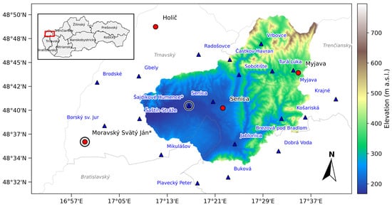
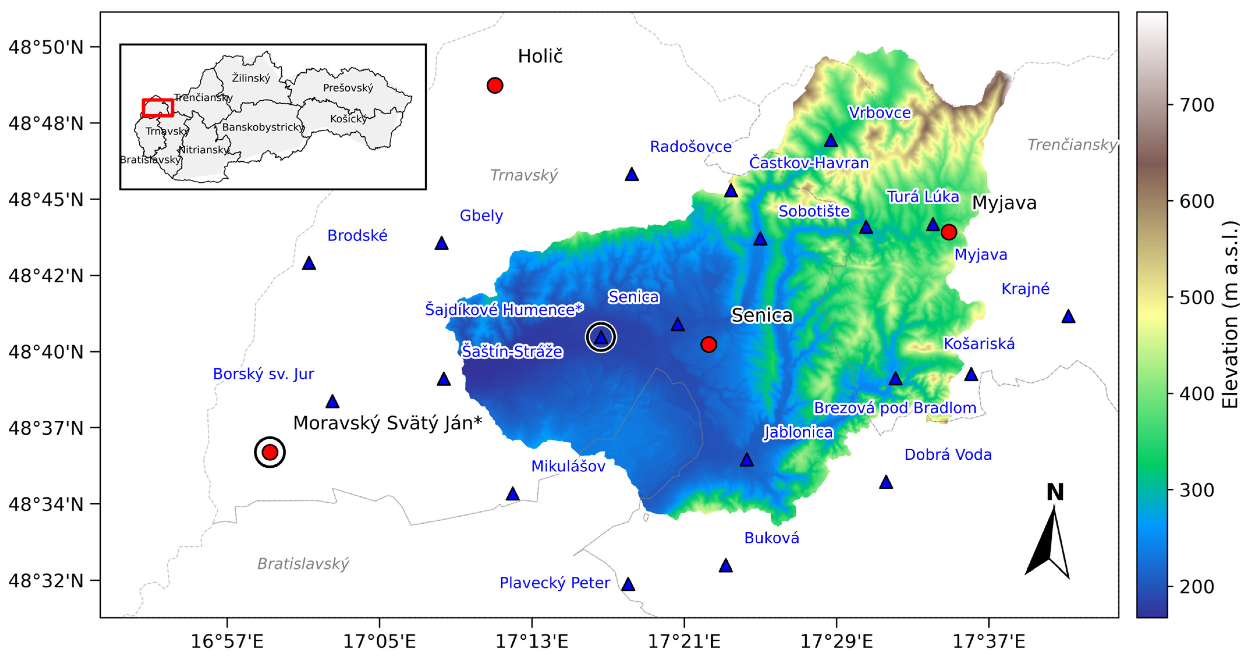
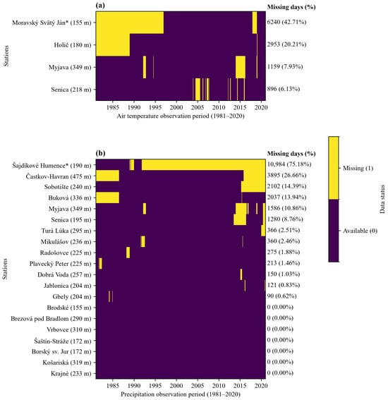
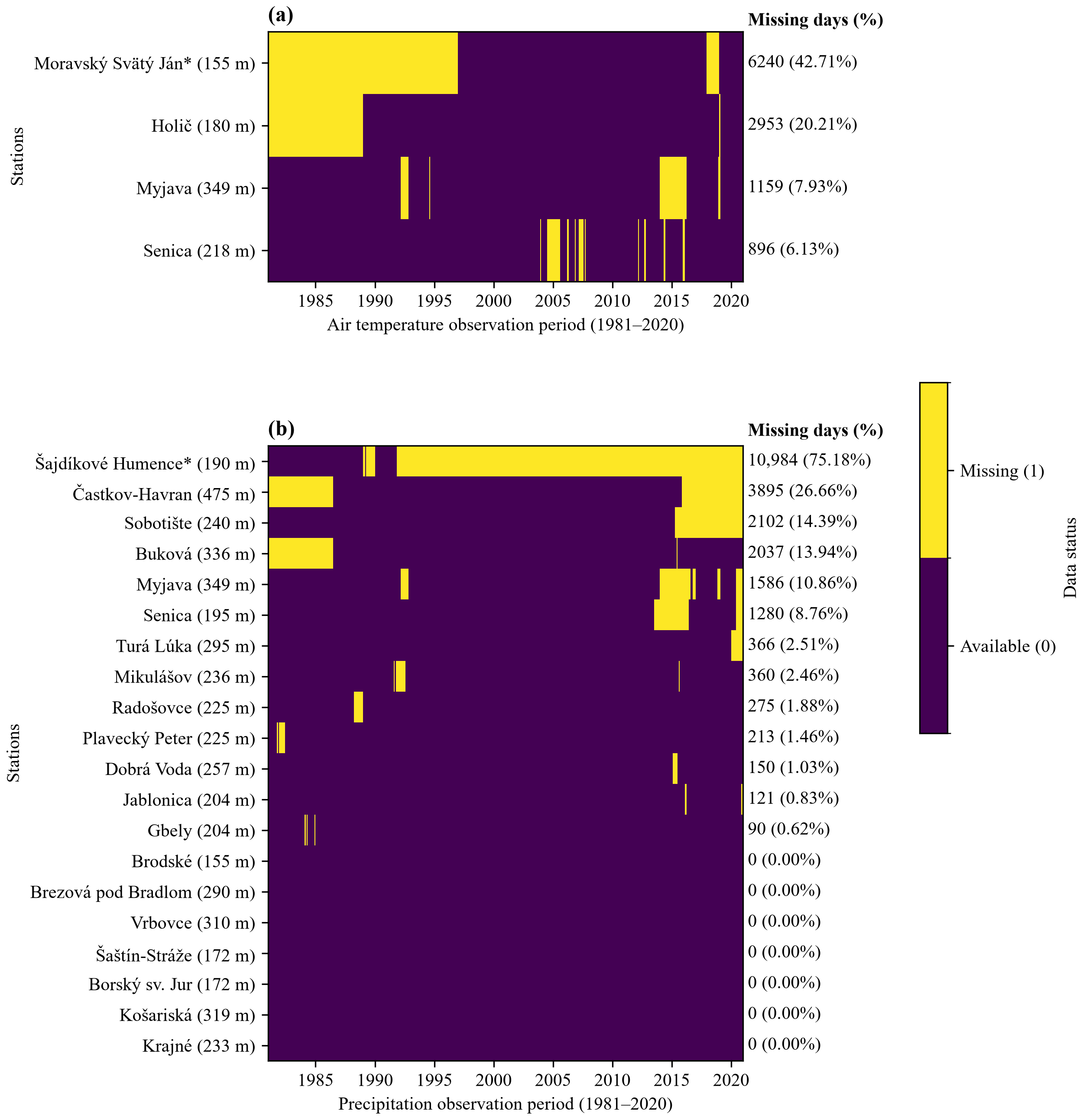
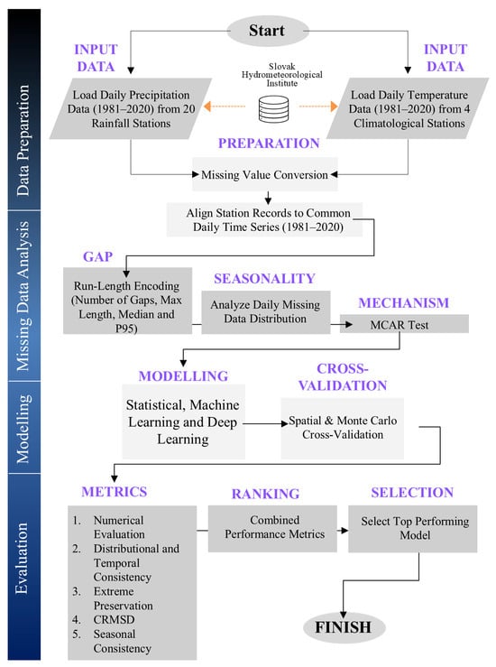
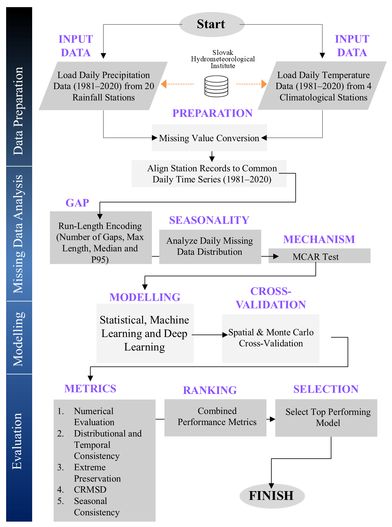
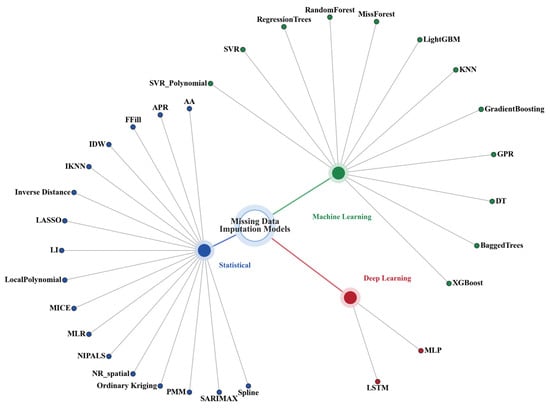

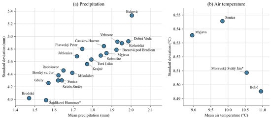
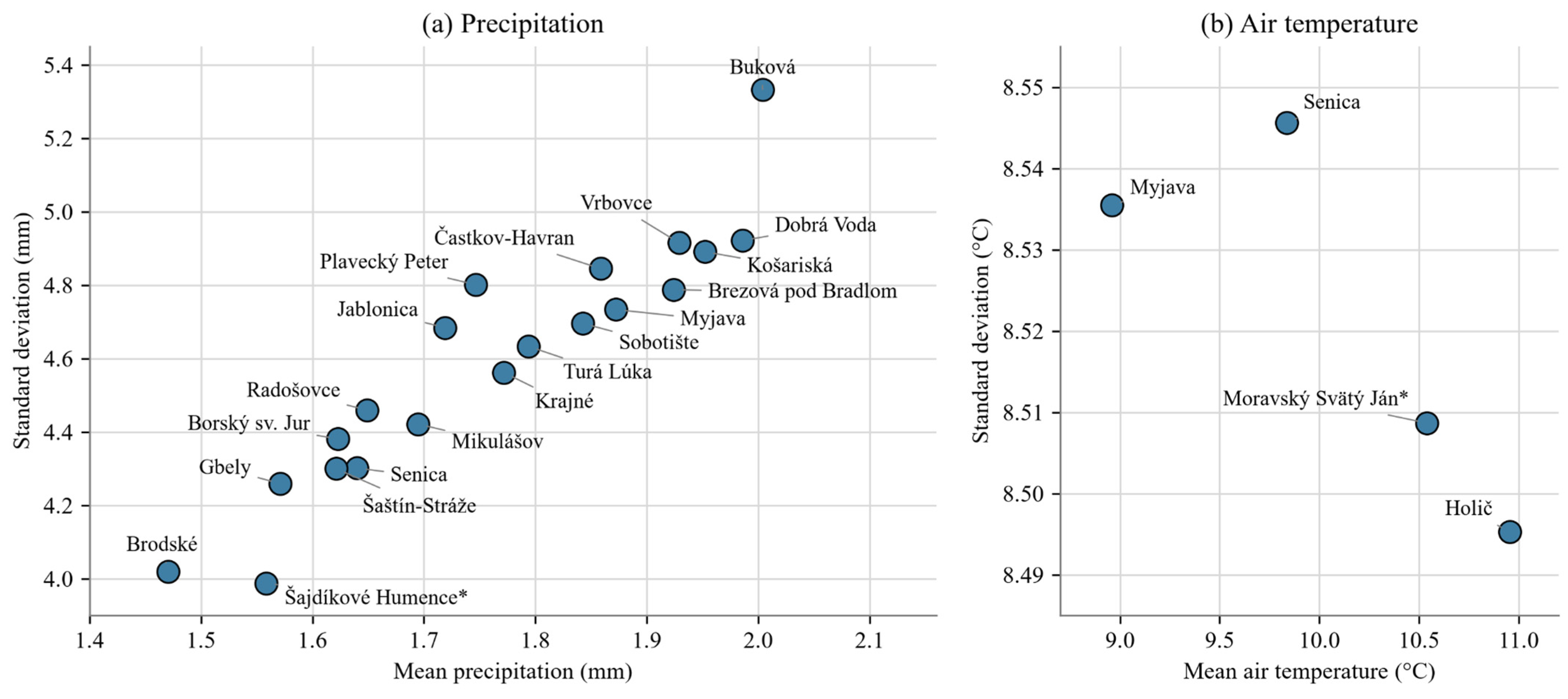
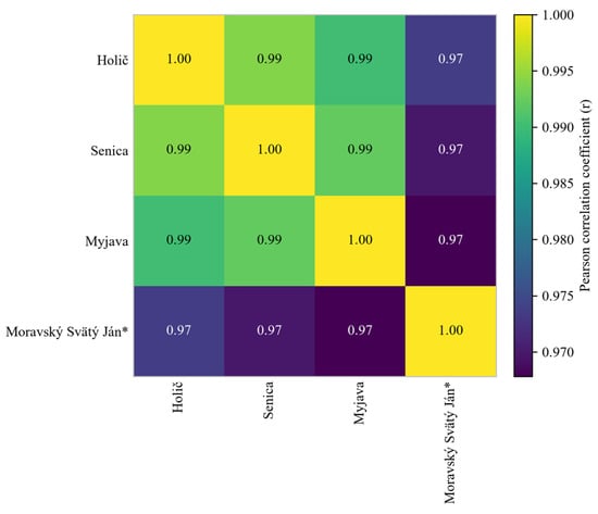
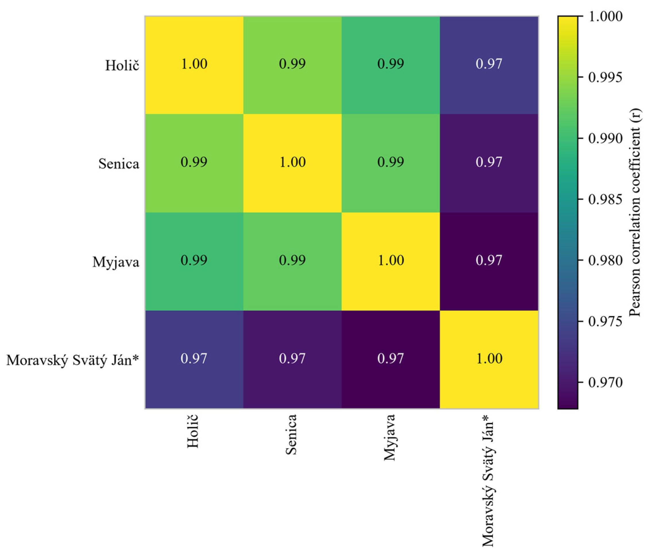
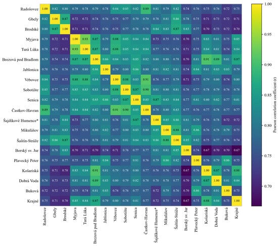
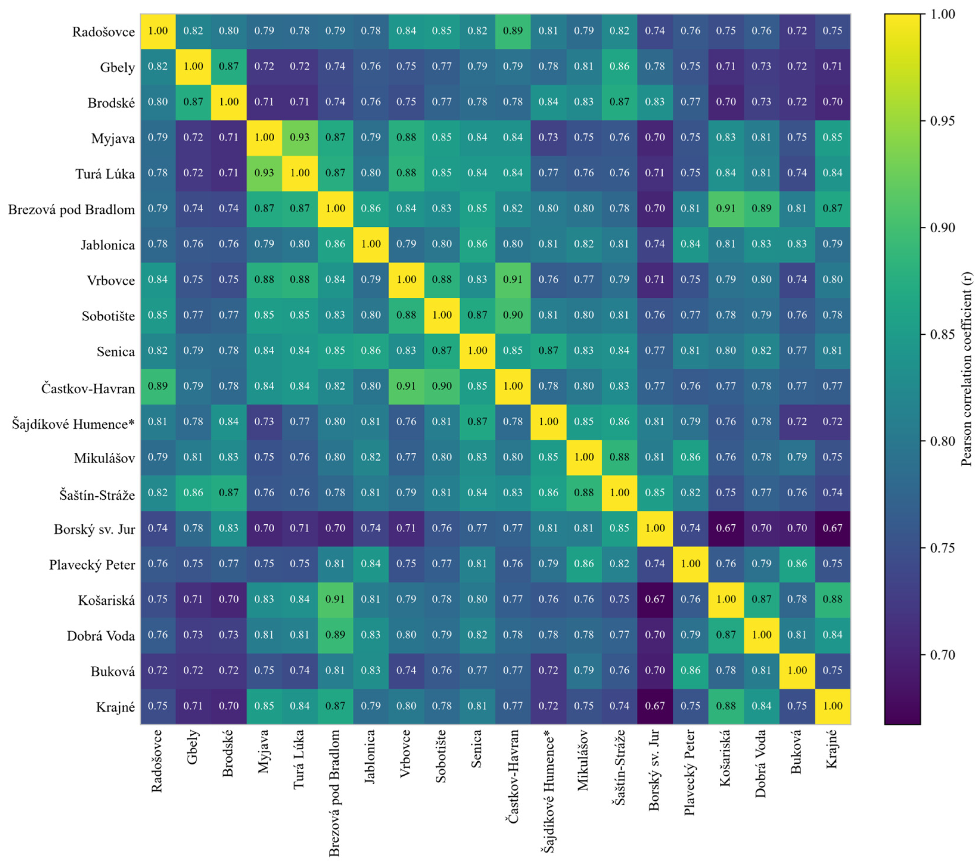
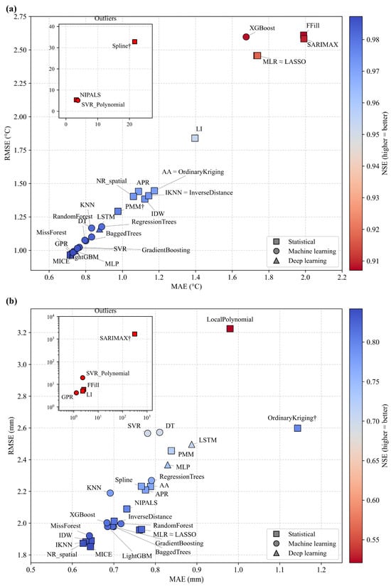
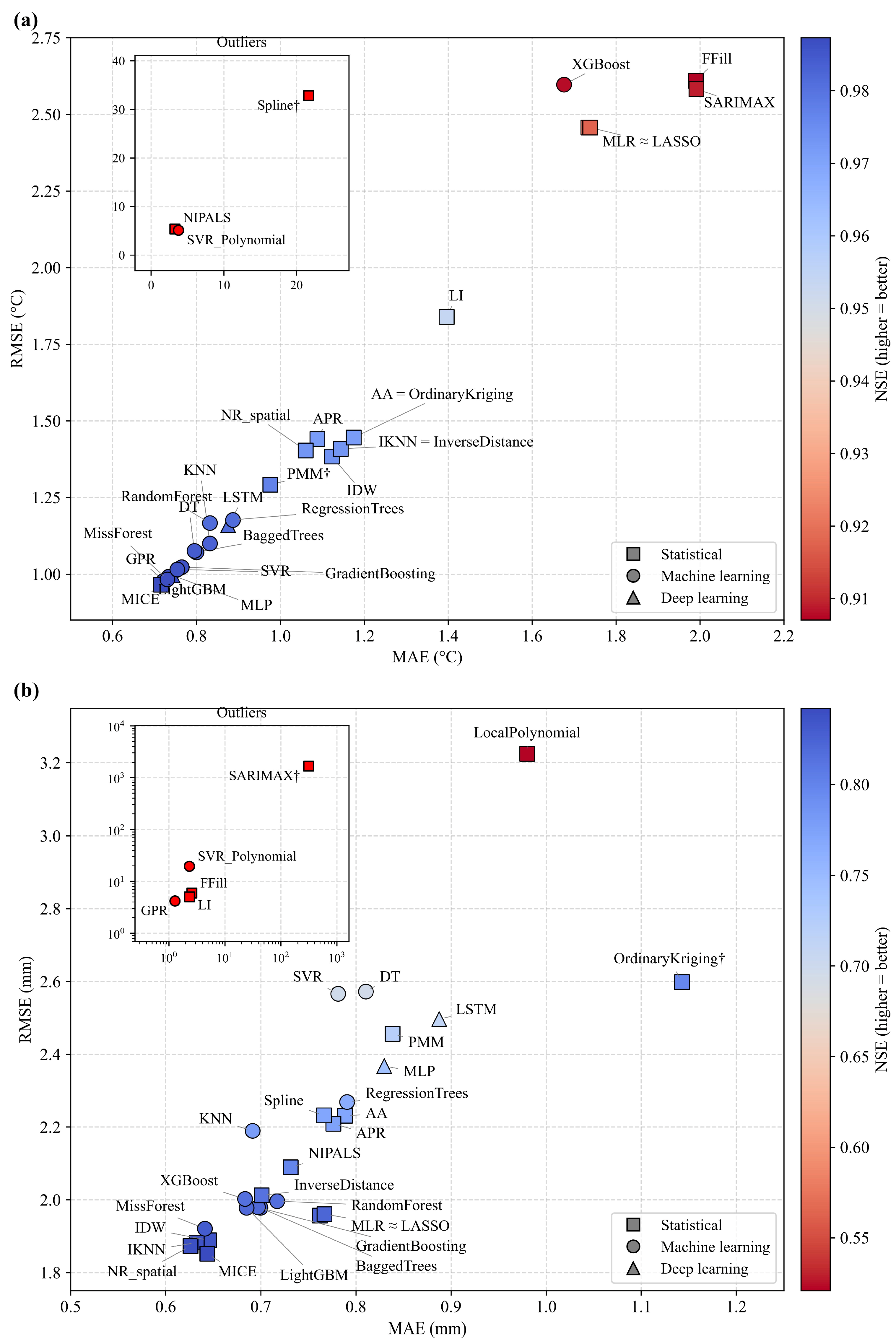
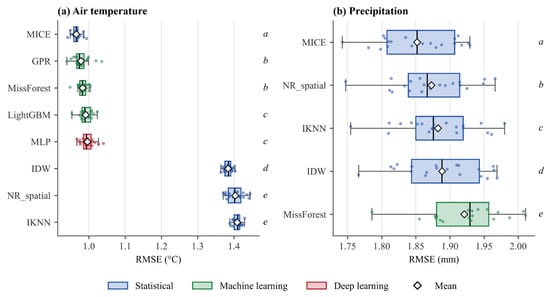
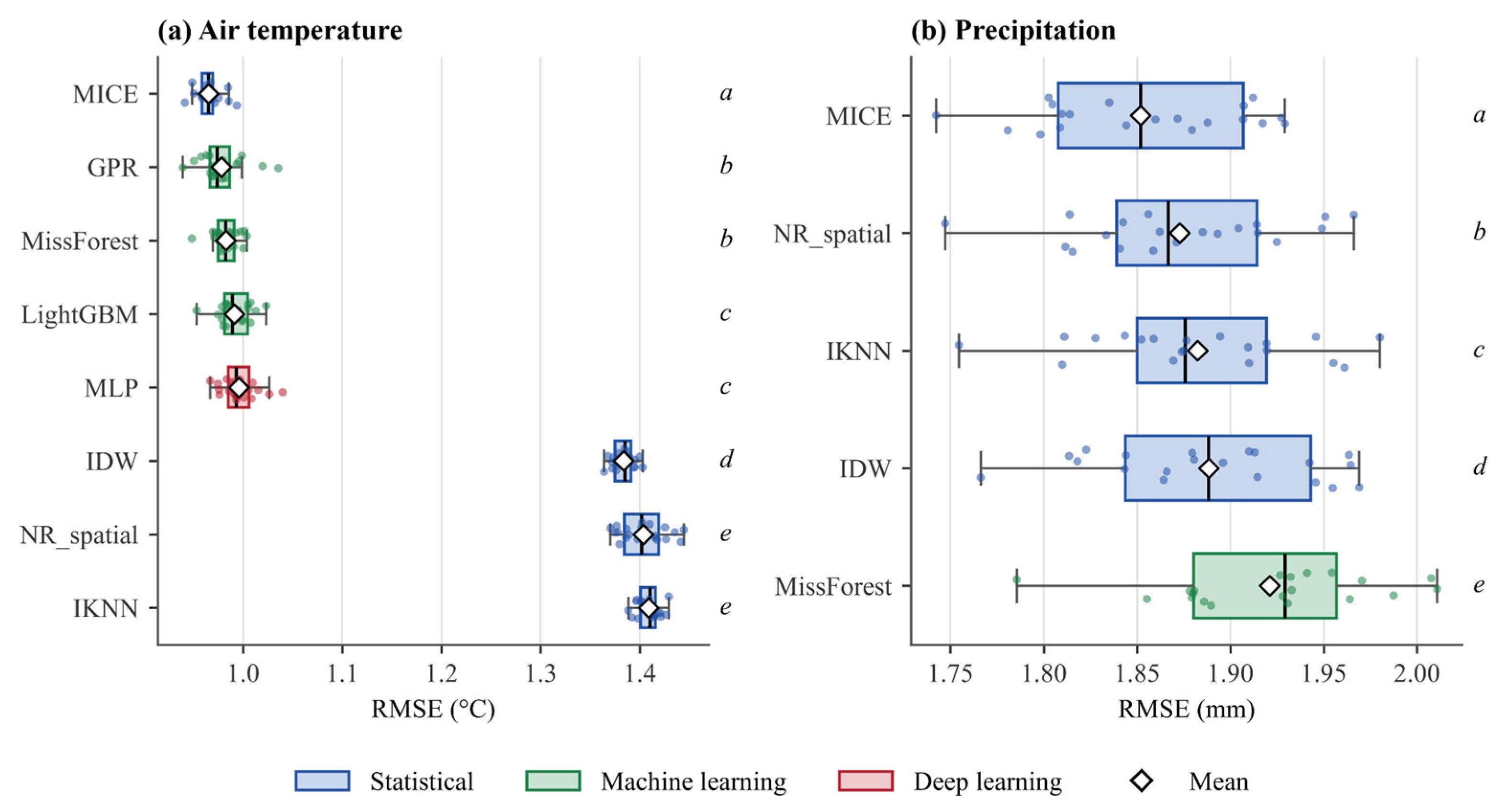
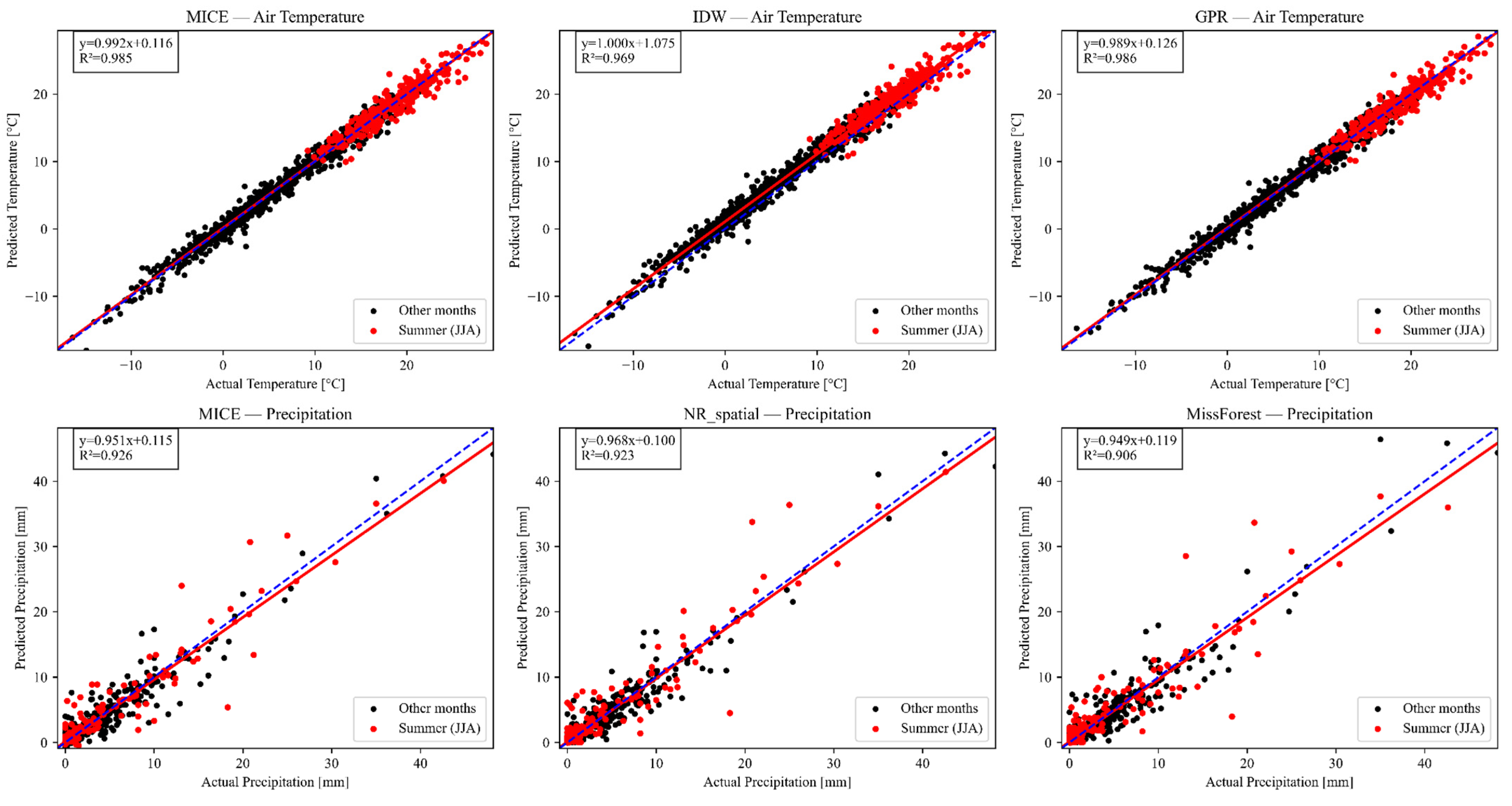
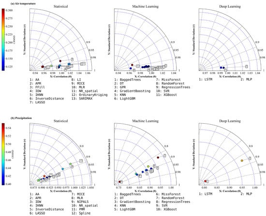
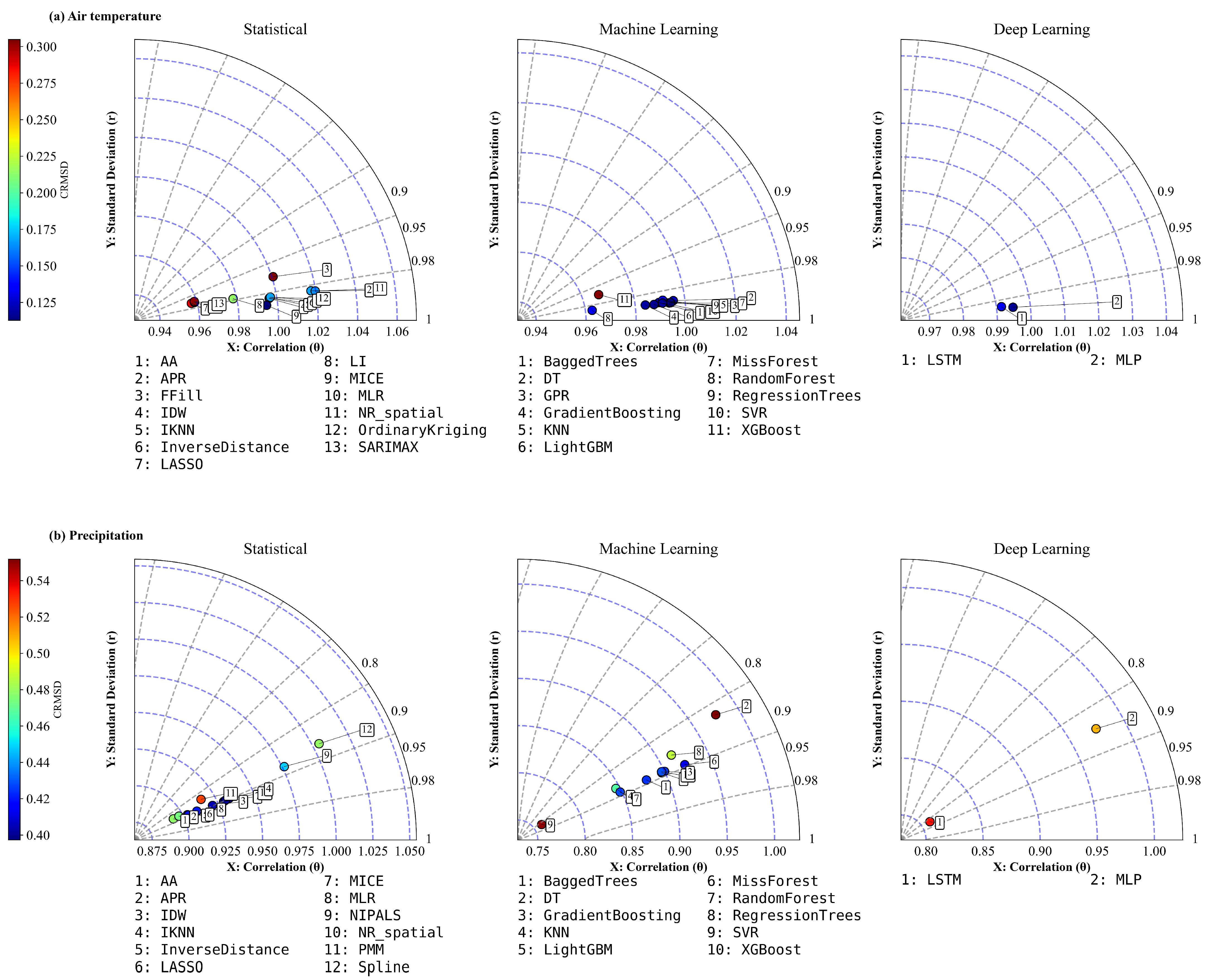

Disclaimer/Publisher’s Note: The statements, opinions and data contained in all publications are solely those of the individual author(s) and contributor(s) and not of MDPI and/or the editor(s). MDPI and/or the editor(s) disclaim responsibility for any injury to people or property resulting from any ideas, methods, instructions or products referred to in the content. |
© 2026 by the authors. Licensee MDPI, Basel, Switzerland. This article is an open access article distributed under the terms and conditions of the Creative Commons Attribution (CC BY) license.