


Abstract
Dissipation can fundamentally reconstruct the multicritical structure of driven-dissipative light–matter systems. In the interpolating Dicke–Tavis–Cummings model, cavity loss eliminates the -symmetric superradiant phase on the Tavis–Cummings line and splits the original multicritical point into a pair of dissipation-induced tricritical points. Here, we show that intracavity optical squeezing provides a coherent means of continuously reshaping this loss-generated multicritical structure. The single-mode parametric interaction acts asymmetrically on the two cavity quadratures, thereby deforming the phase boundaries and continuously tuning the dissipation-induced tricritical points. We analytically determine the phase boundaries and the evolution of the tricritical structure with the parametric gain and cavity dissipation, and show that the two tricritical points coalesce in the weak-loss limit. Photon-number fluctuations provide clear quantum signatures of the squeezing-controlled multicritical structure.
1. Introduction
Understanding quantum phase transitions and criticality is a central topic in modern condensed matter physics and quantum optics [1,2]. A paradigmatic example is the superradiant phase transition in Dicke-type models, where an ensemble of two-level systems collectively interacts with a single bosonic cavity mode [3,4]. When the atom–field coupling strength exceeds a critical value , the system undergoes a transition from the normal phase to a superradiant phase [5,6,7,8,9,10,11,12,13,14]. Beyond conventional critical points, multicritical structures have attracted considerable attention. Of particular interest are tricritical points (TCPs) [15,16,17,18] where the first- and second-order phase transition boundaries meet. In addition to their fundamental importance in nonequilibrium many-body physics, multicritical regimes are expected to enhance the response of a system to external perturbations [19] and therefore offer potential applications in quantum sensing and metrology [20,21,22,23,24,25,26].
A paradigmatic model exhibiting such multicritical behavior is the interpolating Dicke–Tavis–Cummings (IDTC) model [27]. In this model, the two quadratures of a single cavity field couple independently to two orthogonal components of a collective spin, with coupling strengths and . A key feature of the IDTC model is the emergence of a continuous symmetry along the Tavis–Cummings line (), where the normal phase and two superradiant phases meet at a tricritical point.
Realistic light–matter systems are inevitably coupled to their environment. Remarkably, even infinitesimal cavity dissipation fundamentally reconstructs the phase diagram [28,29,30,31,32], destroying the -symmetric superradiant phase on the Tavis–Cummings line and opening a normal-phase sliver between the two Dicke-like superradiant phases [33]. Consequently, the original multicritical point splits into two nonequilibrium tricritical points. However, once the system is fixed, the cavity decay rate is generally difficult to tune by external fields.
Optical squeezing and parametric driving have been explored as effective means of controlling critical phenomena in light–matter systems. In particular, intracavity squeezing has been shown to induce symmetry-breaking superradiant transitions in Tavis–Cummings-type systems [34], and squeezed-light-induced phase transitions have also been studied in the Jaynes–Cummings model [35,36]. More recently, squeezing-assisted multicritical phenomena have been explored in other cavity-QED configurations [37,38]. In contrast to these studies, which focus on squeezing-induced superradiant transitions or tricriticality, the present work addresses the coherent control of a tricritical pair generated by cavity dissipation.
In this work, we introduce intracavity optical parametric amplification into the dissipative IDTC model to achieve coherent control of the dissipation-induced multicritical structure. A classically pumped nonlinear medium generates a coherent two-photon term of the form , where the parametric gain G is controlled by the external pump amplitude [39,40,41,42]. The squeezing interaction reduces the continuous symmetry on the Tavis–Cummings line to the discrete symmetry, allowing superradiant solutions to reappear on this line, consistent with the squeezing-induced symmetry-breaking mechanism reported previously [34]. The coherent interaction continuously changes the superradiant phase boundaries and displaces the two dissipation-induced tricritical points in the plane. We derive the first- and second-order phase boundaries and obtain explicit expressions for the locations of both tricritical points as functions of G and . We further show that finite squeezing breaks the exchange symmetry and asymmetrically deforms the tricritical pair, whereas the two points coalesce in the weak-loss limit. We further characterize their evolution through photon-number fluctuations.
The remainder of this paper is organized as follows. In Section 2, we introduce the dissipative interpolating Dicke–Tavis–Cummings model with intracavity optical parametric amplification, discuss its symmetry properties, and formulate the corresponding open-system dynamics. In Section 3, we derive the semiclassical steady-state solutions and the analytical phase boundaries, and characterize the resulting superradiant phase diagram. In Section 4, we focus on the tunable tricritical structure, derive the locations of the two tricritical points, and analyze their evolution under variation of the parametric gain and cavity dissipation. In Section 5, we investigate quantum fluctuations around the stable mean-field steady states and identify their signatures near the critical boundaries. Finally, Section 6 summarizes our main results and conclusions.
2. Model
We consider an ensemble of N identical two-level atoms, each coupled to both quadratures of a bosonic mode (e.g., the electric and magnetic field components of an electromagnetic field) that contains a second-order nonlinear crystal. Such two-quadrature light–matter couplings can, in principle, be engineered in circuit-QED architectures, where artificial atoms couple capacitively and inductively to a resonator, or through cavity-assisted Raman interaction channels [10,27]. The nonlinear medium is driven by a strong classical pump field with frequency , giving rise to intracavity optical parametric amplification (OPA) [34,37,38,41,42]. Setting , the effective Hamiltonian in the rotating frame at half the pump frequency, , is
where a () denotes the annihilation (creation) operator of the cavity mode, and are the collective spin operators, with the Pauli matrices for the jth atom. The parameters and characterize the anisotropic light–matter couplings. The effective parametric gain is given by , where is the coherent pump amplitude and denotes the effective three-wave-mixing strength. The effective parametric gain G can be continuously controlled through the amplitude of the external pump field. It therefore provides an experimentally accessible coherent control parameter for tuning the phase structure while the cavity dissipation rate is kept fixed. The cavity and atomic detunings are defined as and , respectively, where and denote the bare cavity-mode frequency and the atomic transition frequency, respectively.
For , the symmetry of the Hamiltonian is determined by the anisotropy of the light–matter coupling. Along the Tavis–Cummings line, , the counterrotating terms vanish, and the total excitation number is conserved. The Hamiltonian is invariant under the continuous transformation which gives rise to a symmetry. Away from the Tavis–Cummings line, , the counterrotating terms break excitation-number conservation, reducing the continuous symmetry to the discrete symmetry generated by The parametric drive explicitly breaks the symmetry even along the Tavis–Cummings line. Under the transformation , the two-photon terms acquire phase factors and are therefore not invariant for a general . The discrete symmetry, however, remains preserved because is invariant under . Thus, the OPA reduces the continuous symmetry to . Meanwhile, the parametric drive acts differently on the two cavity quadratures, which are governed by the effective coefficients and , respectively. This quadrature-dependent renormalization provides the microscopic origin of the asymmetric deformation of the phase boundaries discussed below.
We now turn to the open-system dynamics by incorporating cavity photon loss. In contrast to the closed system, where the phase structure is determined solely by the effective Hamiltonian, the steady states of the driven–dissipative system arise from the competition between coherent light–matter interactions, parametric driving, and dissipation. Within the Markovian approximation, the system dynamics is governed by the Lindblad master equation
where denotes the cavity decay rate.
3. Steady-State Phase Diagram
To determine the steady-state phase structure, we first derive the semiclassical equations of motion. In the thermodynamic limit, we introduce the variables where . Factorizing mixed atom–field correlations as , the equations of motion become
The OPA introduces a quadrature-dependent modification of the semiclassical dynamics, with and governed by the effective coefficients and , respectively.
The collective spin length is conserved within the mean-field approximation,
The steady states are obtained by setting the time derivatives in Equation (3) to zero together with the spin-length constraint. The normal-phase solution is
For a superradiant steady state, eliminating the spin components from the stationary mean-field equations gives (see details in Appendix A.1)
Solving for the spin polarization gives two formal branches,
with
Mathematically, determines the boundaries at which the two formal superradiant stationary branches coalesce. The physically relevant segments become discontinuous transition boundaries when the dynamically stable solution terminates with a finite order parameter, as confirmed by the linear-stability analysis in Appendix B and by the cuts shown below.
Real superradiant stationary solutions require . Introducing
the condition yields two branches,
which together define the discontinuous (first-order) transition boundary. In addition to the phase boundaries, the analytic form of the superradiant solution changes across
where the two analytic representations of the superradiant branch exchange their roles, as detailed in Appendix A.1. We refer to Equation (11) as the branch-exchange line; it does not by itself represent a phase-transition boundary.
Throughout this work, we restrict the parametric drive to the below-threshold regime , for which the uncoupled parametrically driven cavity possesses a stable stationary state. This condition also ensures that is real. All parameter sets considered below satisfy this condition. The continuous normal-to-superradiant transition is reached when the stable superradiant branch continuously merges with the normal state, i.e., when . Substituting into Equation (6) yields
which determines the continuous (second-order) transition boundary. Solving Equation (12) for gives
Physical superradiant states are further constrained by dynamical stability. For the parameter regimes considered here, the branch is dynamically stable, whereas the branch is unstable; see Appendix B. In the following, we retain only the stable branch.
To visualize the steady-state phase structure, we use the real and imaginary parts of the cavity field, and , as the superradiant order parameters. For a given stable polarization , these amplitudes are obtained from the stationary mean-field equations together with the spin-length constraint; their explicit expressions are given in Appendix A.1.
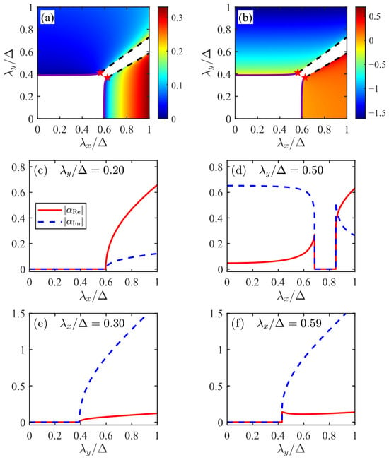
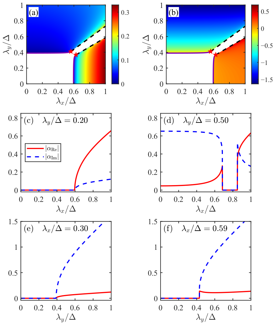
We now examine the mean-field phase structure in the coupling plane. Figure 1a,b show the real and imaginary components of the cavity order parameter, and , respectively. The black dashed lines denote the first-order phase-transition boundaries, while the solid purple curves indicate the second-order transition boundaries. The two types of boundaries meet at the tricritical points, marked by red stars. For , the exchange symmetry is explicitly broken, so that the diagonal no longer serves as a symmetry axis of the phase diagram. This asymmetry originates from the opposite OPA-induced shifts and of the two cavity quadratures. Consequently, the superradiant regions on the two sides of the diagonal become inequivalent.
Figure 1.
Mean-field phase diagram in the plane. (a,b) Real and imaginary parts of the cavity order parameter, and , respectively. The black dashed lines indicate the first-order superradiant phase transition boundaries, and the solid purple curves denote the second-order phase transition boundary. The red stars indicate the tricritical points. The white region corresponds to the normal phase with . (c,d) Order parameters as functions of for fixed and , respectively. (e,f) Corresponding cuts as functions of for fixed and . Here , , and .
The one-dimensional cuts in Figure 1c–f make the distinction between the continuous and discontinuous phase boundaries more explicit. For [Figure 1c], both components of the cavity order parameter remain zero up to and then increase continuously from zero, indicating a continuous normal-to-superradiant transition. A similar behavior is observed for the complementary cut at [Figure 1e], where the superradiant order parameter emerges continuously at . In contrast, for [Figure 1d], the initially superradiant state terminates abruptly at , where both components of the order parameter drop discontinuously to zero. The system remains in the normal phase over a finite interval and reenters the superradiant phase through another discontinuous transition at , yielding a characteristic SP–NP–SP sequence. Likewise, for [Figure 1f], the order parameter exhibits a finite jump at , providing direct signature of a discontinuous normal-to-superradiant transition.
4. Tunable Tricritical Structure
The discontinuous boundaries in Equation (10) intersect the continuous boundary in Equation (13) at two tricritical points (TCPs). Using the definition of in Equation (9), their coordinates are
and
The detailed derivation of Equations (14) and (15) is given in Appendix A.2.
For and finite cavity loss, the two tricritical points are related by the exchange , reflecting the symmetry of the dissipative IDTC model. A finite parametric drive removes this exchange symmetry and continuously deforms the tricritical pair in the plane.
In the weak-loss limit , the two tricritical points coalesce at
In the absence of parametric driving, , Equation (16) is reduced to , with
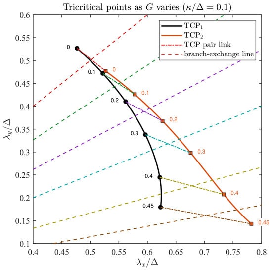
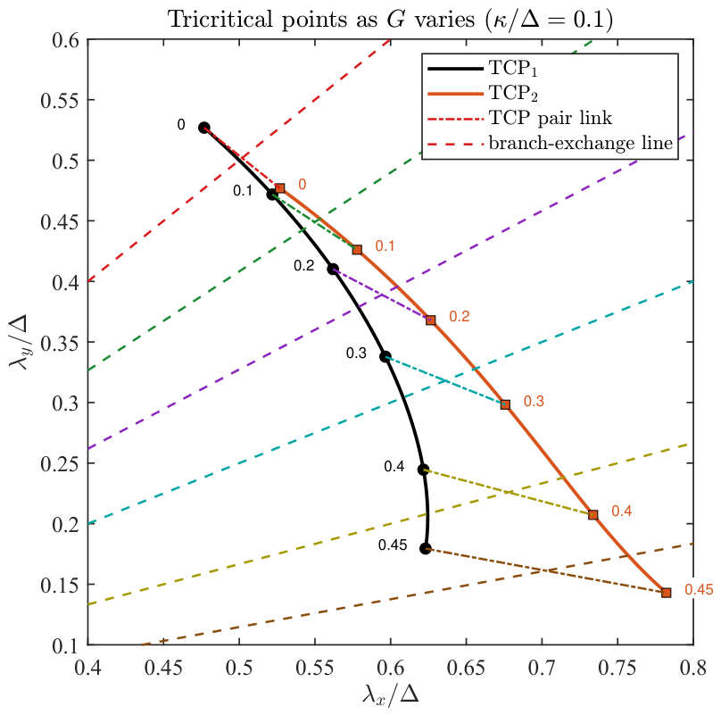
Figure 2 illustrates the resulting evolution of the tricritical structure as the squeezing strength G is varied. At , the two tricritical points form a pair symmetric about the diagonal . Increasing G breaks this symmetry: one tricritical point is displaced toward larger and smaller , whereas the other moves toward smaller and larger . Simultaneously, the branch-exchange line (denoted by the dashed line) in Equation (11) is shifted away from the diagonal. Therefore, the optical squeezing provides an independent control parameter for continuously reshaping the dissipation-induced multicritical structure.
Figure 2.
Evolution of the tricritical points in the plane as the parametric-drive strength G is varied. The black circles and orange squares denote the trajectories of and , respectively, with the adjacent numbers indicating . For each value of G, the dot-dashed line connects the corresponding pair of tricritical points, while the dashed line indicates the branch-exchange line . The parameters are the same as in Figure 1.
The full control space is three dimensional, . To visualize the pump-driven evolution while retaining both tricritical points in a single two-dimensional section, we introduce a fixed coupling-space trajectory:
The line is chosen to pass through the two tricritical points at the reference parameters , , and . This gives as derived explicitly in Appendix A.2. Varying moves the system along this fixed trajectory in the coupling plane, whereas varying G tracks the deformation of the phase structure induced by the parametric drive. Consequently, the original three-dimensional parameter space is represented by the reduced plane shown in Figure 3. Unless otherwise specified, , , and .
Figure 3.
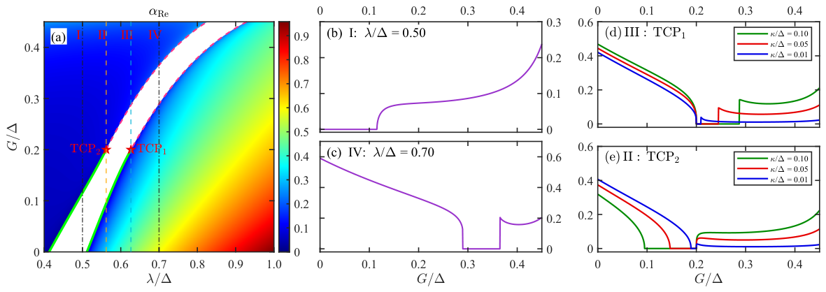
Mean-field order parameter in the plane along the linear cut defined in Equation (17). (a) Real part of the cavity order parameter, . The white region denotes the normal phase with , while the colored regions correspond to superradiant solutions. The vertical dash-dotted lines labeled I–IV indicate representative values of , and the locations of and are marked by red stars. (b,c) Evolution of with the parametric-drive strength G at fixed and , respectively. (d,e) Order-parameter profiles associated with and for different cavity decay rates , , and . Other parameters are the same as in Figure 1.
Figure 3a shows the real part of the cavity order parameter, , in the reduced plane along the linear trajectory defined in Equation (17). The white region corresponds to the normal phase, while a finite indicates the superradiant phase. The four vertical cuts I–IV are chosen according to their positions relative to the two tricritical points: cut I lies to the left of , cuts II and III pass through the vicinity of and , respectively, and cut IV lies to the right of .
The corresponding one-dimensional cuts reveal qualitatively distinct behaviors. At [Figure 3b], the cavity field remains zero at weak parametric driving and develops continuously beyond a critical value of G, indicating a transition from the normal to the superradiant phase. By contrast, for [Figure 3c], the system is in superradiant phase at weak driving, enters a finite normal-phase window at intermediate G, and returns to a superradiant state upon further increasing the parametric strength. Thus, the OPA can either induce or suppress superradiance depending on the position along the coupling-space trajectory, leading to a characteristic reentrant SP–NP–SP structure.
The effect of cavity dissipation is further illustrated in Figure 3d,e, where is fixed at the values corresponding to and , respectively, for the reference loss . For the cut [Figure 3d], a finite normal-phase window opens on the high-G side of the reference point . As is reduced from to , the upper boundary of this window moves toward , so that the normal-phase interval progressively narrows. The complementary evolution is observed for the cut [Figure 3e]. Here the normal-phase window extends toward lower G, and decreasing shifts its lower boundary toward . Thus, the normal-phase regions associated with the two tricritical points contract from opposite sides as the cavity loss is reduced. This behavior directly illustrates the dissipative origin of the splitting between the two tricritical points and their coalescence in the weak-loss limit.
5. Quantum Fluctuation Signatures
Having determined the stable mean-field steady states, we now investigate the quantum fluctuations around them. In the thermodynamic limit, the collective spin is represented by a Holstein–Primakoff boson , We then expand the cavity and collective-spin fields around their mean-field values according to where c and d describe the cavity and atomic quantum fluctuations, respectively. Because the mean-field amplitudes satisfy the steady-state equations, all linear terms in the fluctuation operators c and d vanish, leaving the terms of order to define the quadratic fluctuation Hamiltonian. Up to quadratic order, the fluctuation Hamiltonian can be written as
where and depend on the mean-field solution . Their explicit expressions are given in Appendix C. The OPA contribution appears explicitly as the single-mode squeezing term , and therefore modifies the cavity fluctuation spectrum.
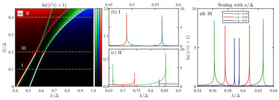
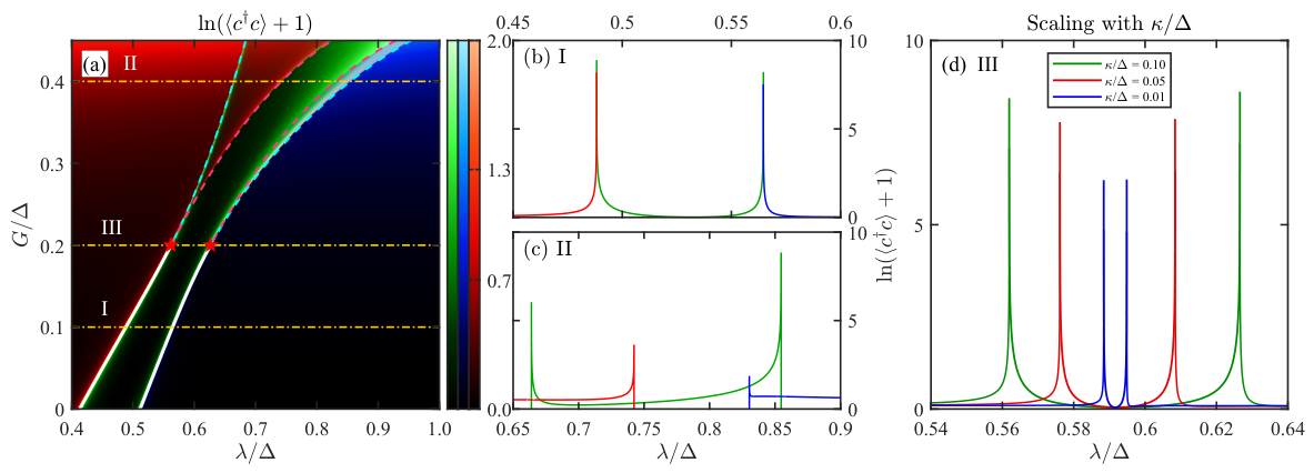
To characterize the phase diagram in open-system dynamics, we use Heisenberg’s equation of motion to obtain a closed set of ten linear equations for the second-order correlators: , , , , , , , , , and (see Appendix D). Their stationary values are obtained by setting all ten time derivatives to zero. As a measure of the cavity fluctuations, we consider the photon number , where c denotes the fluctuation operator around the macroscopic cavity field. Figure 4a shows in the reduced plane along the linear cut defined in Equation (17). The logarithmic scale is introduced to display the large variation of the fluctuation amplitude near the phase boundaries. Away from the critical regions, remains small, while strong fluctuation enhancement occurs near the analytical phase boundaries.
Figure 4.
Photon-number fluctuations along the linear cut defined in Equation (17). (a) in the plane. Separate color scales are used for the normal phase and the two superradiant branches. The dashed curves denote the first-order phase boundaries, while the solid white curves indicate the second-order phase boundaries. The horizontal lines mark cuts I–III at , , and , respectively. (b,c) Photon-number fluctuations along cuts I and II, respectively. (d) Photon-number fluctuations along cut III for , , and . Other parameters are the same as in Figure 1.
Figure 4b,c further illustrate the fluctuation behavior across the two types of phase transitions. Along cut I [Figure 4b], the system crosses two second-order phase boundaries, at which the photon-number fluctuation is strongly enhanced and develops sharp peaks. These peak positions coincide with the continuous normal-to-superradiant transitions identified from the mean-field order parameter. In contrast, cut II [Figure 4c] crosses first-order phase boundaries. In this case, the fluctuation behavior changes abruptly across the transition points, consistent with the finite jumps of the mean-field order parameter. The fluctuation profiles provide a clear distinction between the continuous and discontinuous transitions in the phase diagram.
The effect of cavity dissipation is illustrated in Figure 4d, where cut III is shown for several values of . For finite cavity loss, the two critical boundaries appear as two well-separated fluctuation peaks. As is reduced, the peaks move progressively toward one another and the interval between them becomes narrower. This evolution mirrors the shrinking normal-phase region found in the mean-field phase diagram and is consistent with the coalescence of the dissipation-induced tricritical structure in the weak-loss limit. Thus, the photon-number fluctuation provides a direct quantum signature of the dissipation-induced splitting and its coherent control by the parametric drive.
These signatures are directly relevant to experimental measurements. The cavity order parameter can be accessed through the coherent component of the output field. Through the standard input–output relation [43], the intracavity fluctuation quantity considered above is directly related to fluctuations of the cavity output field [8,44] and can be probed by photon counting or homodyne detection [45]. From an experimental perspective, the relevant signature is the displacement and enhancement of the fluctuation peaks as the parametric pump strength is varied. These output-field observables provide a possible route for identifying the squeezing-controlled evolution of the multicritical structure.
6. Conclusions
In summary, we have investigated the coherent control of dissipation-induced multicriticality in the interpolating Dicke–Tavis–Cummings model by intracavity optical squeezing. The parametric interaction acts differently on the two cavity quadratures and thereby provides a coherent method for continuously reshaping this loss-generated tricritical structure. Within the mean-field approximation, we obtained the steady-state solutions and the corresponding phase boundaries analytically. We showed that the parametric drive continuously displaces the dissipation-induced pair of tricritical points whose positions can be controlled by the pump strength. We further studied quantum fluctuations around the stable mean-field steady states using a Holstein–Primakoff expansion and the corresponding quadratic fluctuation dynamics. The intracavity parametric interaction enters directly as a single-mode squeezing term in the fluctuation Hamiltonian and strongly modifies the cavity fluctuation spectrum.
Author Contributions
Conceptualization, Y.H. and G.-L.Z.; methodology, Y.H. and G.-L.Z.; software, Y.H.; writing—original draft preparation, Y.H. and G.-L.Z.; writing—review and editing, L.C., G.-L.Z. and X.W.; supervision, G.-L.Z. and L.C.; funding acquisition, project administration, G.-L.Z. and X.W. All authors have read and agreed to the published version of the manuscript.
Funding
This work is supported by the National Natural Science Foundation of China (Grant No. 12405027), the Zhejiang Provincial Natural Science Foundation of China (Grant No. LQN25A050001), the Quantum Science and Technology–National Science and Technology Major Project (Grant No. 2024ZD0301000), and the Science Foundation of Zhejiang Sci-Tech University (Grant Nos. 24062156-Y and 23062088-Y).
Data Availability Statement
The data supporting the findings of this study are available from the corresponding authors upon reasonable request.
Conflicts of Interest
The authors declare no conflicts of interest.
Abbreviations
The following abbreviations are used in this manuscript:
| IDTC | Interpolating Dicke–Tavis–Cummings |
| OPA | Optical parametric amplification |
| NP | Normal phase |
| SP | Superradiant phase |
| TCP | Tricritical point |
Appendix A. Mean-Field Steady States and Tricritical Structure
This Appendix presents the derivation of the explicit superradiant steady-state amplitudes and the associated branch-exchange condition. We then derive the coordinates of the two tricritical points and construct the linear trajectory used in the reduced phase diagrams.
Appendix A.1. Explicit Superradiant Amplitudes and Branch Exchange
For a chosen polarization Z satisfying Equation (7), the stationary spin equations give
The stationary cavity equations provide an equivalent expression,
It is useful to define
Using the spin-length constraint Equation (4) gives
where
Alternatively, using Equation (A3), one obtains
with
Subtracting Equations (A5) and (A7), and defining
gives
The two analytic ratios are therefore
For either analytic branch, the cavity amplitudes can then be written compactly as
The two values of are related by the parity symmetry and therefore describe the degenerate pair of symmetry-broken steady states. The associated spin components follow directly from Equation (A1). In the parameter regimes used in the main text, dynamical stability selects the polarization branch together with the appropriate analytic continuation of Equation (A11); see Appendix B.
The mixed coefficient controls the coupling between the two cavity quadratures in Equation (A7). For finite cavity loss, the two analytic superradiant continuations exchange their labeling when this mixed term vanishes,
Using Equation (A8b), this condition becomes
or
which reproduces the branch-exchange line Equation (11) in the main text.
Appendix A.2. Tricritical Points and Construction of the Linear Cut
The tricritical points are obtained by intersecting the two superradiant-existence boundaries with the continuous normal-to-superradiant boundary. For compactness, define
The two branches of the existence boundary, Equation (10), can then be parameterized as
Substituting Equation (A17) into the continuous-boundary condition, Equation (12), gives
The choice gives TCP1, whereas gives TCP2. Equation (A18) therefore reproduces Equations (14) and (15) of the main text.
Several limiting cases follow immediately. For , , and the two points satisfy
so that the tricritical pair is symmetric about for finite .
In the weak-loss limit,
the two solutions of Equation (A18) coalesce at
which is Equation (16). For this further reduces to .
We finally construct the linear trajectory used in Figure 3 and Figure 4. For the reference parameters , , and , Equations (14) and (15) give
and
The slope of the straight line passing through these two points is therefore
and its dimensionless intercept is
Hence the fixed trajectory is
which is Equation (17) in the main text.
Appendix B. Linear Stability Analysis
Let each mean-field variable be written as its stationary value plus a small fluctuation. The spin constraint eliminates the longitudinal component:
For , the linearized dynamics is , where
A fixed point is linearly stable when every eigenvalue of satisfies ; a phase boundary is reached when the largest real part becomes zero.
For the normal fixed point , Equation (A28) reduces to
For a superradiant phase, the solutions in Equation (A12) are substituted into Equation (A28) before diagonalization. Figure A1 shows the linear stability in plane. The normal-phase solution is stable only in the finite region shown in Figure A1a, and the stability of the superradiant phase is shown in Figure A1b. The boundaries of these regions are determined by the condition , where are the eigenvalues of the linearized stability matrix. In particular, the loss-induced normal-phase strip identified from the stability analysis agrees closely with that obtained from the mean-field order parameter.
Figure A1.
Linear-stability diagrams in the plane for (a) the normal phase and (b) the superradiant branch. Green regions indicate dynamically stable steady states, for which all eigenvalues of the corresponding stability matrix have negative real parts. White regions denote parameter regimes where the considered steady state is unstable. Only the superradiant branch is shown in panel (b), since the branch is unstable in the parameter regime considered.
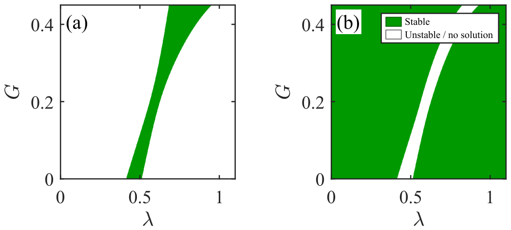
Throughout this work, we use the branch to construct the mean-field phase diagrams and the corresponding fluctuation spectra. As confirmed by the linear-stability analysis, the solutions are dynamically stable in the parameter regimes considered in Figure 3 and Figure 4. By contrast, whenever the branch satisfies the spin constraint, it possesses at least one eigenvalue with a positive real part and is therefore dynamically unstable. The branch is thus excluded from the physical phase diagrams and is not shown.
Appendix C. Holstein–Primakoff Expansion and Fluctuation Coefficients
For a collective spin of length , we introduce a Holstein–Primakoff boson through
We displace the cavity and atomic bosons according to
Expanding the square root in Equation (A30) in powers of , the terms of order vanish when the mean-field equations are satisfied. The terms of order give Equation (18). For the convention in Equation (A31), its coefficients are
At the normal fixed point , these expressions reduce to
The OPA term contributes directly to the quadratic fluctuation Hamiltonian through . The remaining coefficients retain the same functional structure as in the IDTC model, but depend implicitly on G through the G-dependent mean-field steady state.
Appendix D. Equations of Motion for Second-Order Correlations
The equal-time two-operator correlators are obtained directly from Heisenberg’s equation of motion. For example, the cavity photon-number operator obeys
where , and the last term accounts for cavity loss. Evaluating the corresponding commutator for each two-operator product gives the following closed equations of motion:
The constant terms appearing in Equations (A35a)–(A35j) originate from the bosonic commutation relations, such as . For each stable mean-field steady state, we first evaluate the corresponding coefficients and and collect the ten second-order correlators into the vector
The coupled Equations (A35a)–(A35j) can be written in the compact linear form
where is determined by the fluctuation coefficients and contains the constant terms generated by the bosonic commutators. In the stationary state, , and the correlation functions are obtained by solving
The cavity photon-number fluctuation is then extracted from the first component of .
References
- Sachdev, S. Quantum Phase Transitions; Cambridge University Press: Cambridge, UK, 2011. [Google Scholar]
- Domb, C. Phase Transitions and Critical Phenomena; Elsevier: Amsterdam, The Netherlands, 2000. [Google Scholar]
- Dicke, R.H. Coherence in Spontaneous Radiation Processes. Phys. Rev. 1954, 93, 99–110. [Google Scholar] [CrossRef] [Scilit]
- Tavis, M.; Cummings, F.W. Exact Solution for an N-Molecule—Radiation-Field Hamiltonian. Phys. Rev. 1968, 170, 379–384. [Google Scholar] [CrossRef] [Scilit]
- Wang, Y.K.; Hioe, F.T. Phase Transition in the Dicke Model of Superradiance. Phys. Rev. A 1973, 7, 831–836. [Google Scholar] [CrossRef] [Scilit]
- Hioe, F.T. Phase Transitions in Some Generalized Dicke Models of Superradiance. Phys. Rev. A 1973, 8, 1440–1445. [Google Scholar] [CrossRef] [Scilit]
- Emary, C.; Brandes, T. Chaos and the quantum phase transition in the Dicke model. Phys. Rev. E 2003, 67, 066203. [Google Scholar] [CrossRef] [Scilit]
- Dimer, F.; Estienne, B.; Parkins, A.S.; Carmichael, H.J. Proposed realization of the Dicke-model quantum phase transition in an optical cavity QED system. Phys. Rev. A 2007, 75, 013804. [Google Scholar] [CrossRef] [Scilit]
- Nagy, D.; Kónya, G.; Szirmai, G.; Domokos, P. Dicke-Model Phase Transition in the Quantum Motion of a Bose-Einstein Condensate in an Optical Cavity. Phys. Rev. Lett. 2010, 104, 130401. [Google Scholar] [CrossRef] [Scilit]
- Baden, M.P.; Arnold, K.J.; Grimsmo, A.L.; Parkins, S.; Barrett, M.D. Realization of the Dicke Model Using Cavity-Assisted Raman Transitions. Phys. Rev. Lett. 2014, 113, 020408. [Google Scholar] [CrossRef] [Scilit]
- Zhang, G.Q.; Chen, Z.; You, J.Q. Experimentally accessible quantum phase transition in a non-Hermitian Tavis-Cummings model engineered with two drive fields. Phys. Rev. A 2020, 102, 032202. [Google Scholar] [CrossRef] [Scilit]
- Chen, X.Y.; Zhang, Y.Y.; Chen, Q.H.; Lin, H.Q. Phase transitions in the anisotropic Dicke-Stark model with A2 terms. Phys. Rev. A 2024, 110, 063722. [Google Scholar] [CrossRef] [Scilit]
- Zhang, Y.Y.; Hu, Z.X.; Fu, L.; Luo, H.G.; Pu, H.; Zhang, X.F. Quantum Phases in a Quantum Rabi Triangle. Phys. Rev. Lett. 2021, 127, 063602. [Google Scholar] [CrossRef] [Scilit]
- Zheng, R.H.; Ning, W.; Chen, Y.H.; Lü, J.H.; Shen, L.T.; Xu, K.; Zhang, Y.-R.; Xu, D.; Li, H.; Xia, Y.; et al. Observation of a Superradiant Phase Transition with Emergent Cat States. Phys. Rev. Lett. 2023, 131, 113601. [Google Scholar] [CrossRef] [Scilit]
- Xu, Y.; Pu, H. Emergent Universality in a Quantum Tricritical Dicke Model. Phys. Rev. Lett. 2019, 122, 193201. [Google Scholar] [CrossRef] [Scilit]
- Zhu, H.J.; Xu, K.; Zhang, G.F.; Liu, W.M. Finite-Component Multicriticality at the Superradiant Quantum Phase Transition. Phys. Rev. Lett. 2020, 125, 050402. [Google Scholar] [CrossRef] [Scilit]
- Xu, Y.; Fallas Padilla, D.; Pu, H. Multicriticality and quantum fluctuation in a generalized Dicke model. Phys. Rev. A 2021, 104, 043708. [Google Scholar] [CrossRef] [Scilit]
- Ying, Z.J. Symmetry-breaking patterns, tricriticalities, and quadruple points in the quantum Rabi model with bias and nonlinear interaction. Phys. Rev. A 2021, 103, 063701. [Google Scholar] [CrossRef] [Scilit]
- Cheng, J.M.; Zhang, Y.C.; Zhou, X.F.; Zhou, Z.W. Super-Heisenberg Scaling in a Triple-Point Criticality. Phys. Rev. Lett. 2025, 134, 190802. [Google Scholar] [CrossRef] [Scilit]
- Wang, T.L.; Wu, L.N.; Yang, W.; Jin, G.R.; Lambert, N.; Nori, F. Quantum Fisher information as a signature of the superradiant quantum phase transition. New J. Phys. 2014, 16, 063039. [Google Scholar] [CrossRef] [Scilit]
- Frérot, I.; Roscilde, T. Quantum Critical Metrology. Phys. Rev. Lett. 2018, 121, 020402. [Google Scholar] [CrossRef] [Scilit]
- Friedemann, S.; Duncan, W.J.; Hirschberger, M.; Bauer, T.W.; Küchler, R.; Neubauer, A.; Brando, M.; Pfleiderer, C.; Grosche, F.M. Quantum tricritical points in NbFe. Nat. Phys. 2018, 14, 62–67. [Google Scholar] [CrossRef] [Scilit]
- Ying, Z.J.; Felicetti, S.; Liu, G.; Braak, D. Critical Quantum Metrology in the Non-Linear Quantum Rabi Model. Entropy 2022, 24, 1015. [Google Scholar] [CrossRef] [Scilit]
- He, W.T.; Lu, C.W.; Yao, Y.X.; Zhu, H.Y.; Ai, Q. Criticality-based quantum metrology in the presence of decoherence. Front. Phys. 2023, 18, 31304. [Google Scholar] [CrossRef] [Scilit]
- Hotter, C.; Ritsch, H.; Gietka, K. Combining Critical and Quantum Metrology. Phys. Rev. Lett. 2024, 132, 060801. [Google Scholar] [CrossRef] [Scilit]
- Zhu, X.; Lü, J.H.; Ning, W.; Shen, L.T.; Wu, F.; Yang, Z.B. Quantum geometric tensor and critical metrology in the anisotropic Dicke model. Phys. Rev. A 2024, 109, 052621. [Google Scholar] [CrossRef] [Scilit]
- Baksic, A.; Ciuti, C. Controlling Discrete and Continuous Symmetries in “Superradiant” Phase Transitions with Circuit QED Systems. Phys. Rev. Lett. 2014, 112, 173601. [Google Scholar] [CrossRef] [Scilit]
- Kirton, P.; Keeling, J. Suppressing and Restoring the Dicke Superradiance Transition by Dephasing and Decay. Phys. Rev. Lett. 2017, 118, 123602. [Google Scholar] [CrossRef] [Scilit]
- Soriente, M.; Donner, T.; Chitra, R.; Zilberberg, O. Dissipation-Induced Anomalous Multicritical Phenomena. Phys. Rev. Lett. 2018, 120, 183603. [Google Scholar] [CrossRef] [Scilit]
- Lin, R.; Rosa-Medina, R.; Ferri, F.; Finger, F.; Kroeger, K.; Donner, T.; Esslinger, T.; Chitra, R. Dissipation-Engineered Family of Nearly Dark States in Many-Body Cavity-Atom Systems. Phys. Rev. Lett. 2022, 128, 153601. [Google Scholar] [CrossRef] [Scilit]
- Wu, Z.; Hu, C.; Wang, T.; Chen, Y.; Li, Y.; Zhao, L.; Lü, X.Y.; Peng, X. Experimental Quantum Simulation of Multicriticality in Closed and Open Rabi Model. Phys. Rev. Lett. 2024, 133, 173602. [Google Scholar] [CrossRef] [Scilit]
- Xu, Y.J.; Zhai, L.H.; Fu, P.; Cheng, S.J.; Zhang, G.Q. Nonreciprocal quantum phase transition in cavity magnonics. Phys. Rev. A 2024, 110, 043704. [Google Scholar] [CrossRef] [Scilit]
- Kirton, P.; Roses, M.M.; Keeling, J.; Dalla Torre, E.G. Introduction to the Dicke Model: From Equilibrium to Nonequilibrium, and Vice Versa. Adv. Quantum Technol. 2019, 2, 1800043. [Google Scholar] [CrossRef] [Scilit]
- Zhu, C.J.; Ping, L.L.; Yang, Y.P.; Agarwal, G.S. Squeezed Light Induced Symmetry Breaking Superradiant Phase Transition. Phys. Rev. Lett. 2020, 124, 073602. [Google Scholar] [CrossRef] [Scilit]
- Shen, L.-T.; Tang, C.-Q.; Shi, Z.; Wu, H.; Yang, Z.-B.; Zheng, S.-B. Squeezed-Light-Induced Quantum Phase Transition in the Jaynes–Cummings Model. Phys. Rev. A 2022, 106, 023705. [Google Scholar] [CrossRef] [Scilit]
- Lü, J.-H.; Ning, W.; Zhu, X.; Wu, F.; Shen, L.-T.; Yang, Z.-B.; Zheng, S.-B. Critical Quantum Sensing Based on the Jaynes–Cummings Model with a Squeezing Drive. Phys. Rev. A 2022, 106, 062616. [Google Scholar] [CrossRef] [Scilit]
- Zhu, G.L.; Hu, C.S.; Wang, H.; Qin, W.; Lü, X.Y.; Nori, F. Nonreciprocal Superradiant Phase Transitions and Multicriticality in a Cavity QED System. Phys. Rev. Lett. 2024, 132, 193602. [Google Scholar] [CrossRef] [Scilit]
- Song, H.; Zhu, G.L.; Wang, X. Dissipative superradiant phase transitions and multicriticality induced by two-mode squeezing. Phys. Rev. A 2025, 112, 023704. [Google Scholar] [CrossRef] [Scilit]
- Scully, M.O.; Zubairy, M.S. Quantum Optics; Cambridge University Press: Cambridge, UK, 1999. [Google Scholar]
- Agarwal, G.S. Quantum Optics; Cambridge University Press: Cambridge, UK, 2012. [Google Scholar]
- Lü, X.Y.; Wu, Y.; Johansson, J.R.; Jing, H.; Zhang, J.; Nori, F. Squeezed Optomechanics with Phase-Matched Amplification and Dissipation. Phys. Rev. Lett. 2015, 114, 093602. [Google Scholar] [CrossRef] [Scilit]
- Qin, W.; Kockum, A.F.; Muñoz, C.S.; Miranowicz, A.; Nori, F. Quantum amplification and simulation of strong and ultrastrong coupling of light and matter. Phys. Rep. 2024, 1078, 1–59. [Google Scholar] [CrossRef] [Scilit]
- Gardiner, C.W.; Collett, M.J. Input and Output in Damped Quantum Systems: Quantum Stochastic Differential Equations and the Master Equation. Phys. Rev. A 1985, 31, 3761–3774. [Google Scholar] [CrossRef] [Scilit]
- Baumann, K.; Guerlin, C.; Brennecke, F.; Esslinger, T. Dicke Quantum Phase Transition with a Superfluid Gas in an Optical Cavity. Nature 2010, 464, 1301–1306. [Google Scholar] [CrossRef] [Scilit]
- Bina, M.; Amelio, I.; Paris, M.G.A. Dicke Coupling by Feasible Local Measurements at the Superradiant Quantum Phase Transition. Phys. Rev. E 2016, 93, 052118. [Google Scholar] [CrossRef] [Scilit]
Disclaimer/Publisher’s Note: The statements, opinions and data contained in all publications are solely those of the individual author(s) and contributor(s) and not of MDPI and/or the editor(s). MDPI and/or the editor(s) disclaim responsibility for any injury to people or property resulting from any ideas, methods, instructions or products referred to in the content. |
© 2026 by the authors. Licensee MDPI, Basel, Switzerland. This article is an open access article distributed under the terms and conditions of the Creative Commons Attribution (CC BY) license.