Non-Contact Thickness Measurement Using Deep Learning-Assisted 3×3 Fiber-Coupler Laser-Ultrasonic Interferometry

Abstract

Non-contact ultrasonic thickness measurement is important for industrial metrology, particularly for metallic components where surface temperature, motion, geometry, or contamination can limit conventional contact probes. In this study, we present a fully non-contact thickness measurement system for aluminum plates integrating laser-ultrasound excitation, 3×3 interferometric detection, and deep learning-based phase demodulation. Broadband ultrasonic waves were generated using a pulsed 532 nm laser in the ablation regime, while rear-surface displacement was detected using a 1550 nm fiber-optic interferometric probe. Two phase-shifted outputs from a 3×3 coupler were processed by a neural interferometric demodulator (NID), which directly reconstructed continuous optical phase without separate quadrature reconstruction, arctangent phase extraction, or phase unwrapping during inference. PZT-modulated measurements at 10, 15, 20, and 25 kPa provided additional validation against conventional 3×3 standard ellipse fitting (3×3-SEF), including phase excursions exceeding $2\mathsf{\pi }$. The NID reduced the phase RMSE from 0.048 to 0.071 rad to 0.029–0.041 rad and the processing time from 481 ± 22 μs to 295 ± 30 μs per sequence. For thickness measurement, the reconstructed phase was converted into out-of-plane displacement, and acoustic time-of-flight (TOF) features were extracted. For 2, 6, and 10 mm aluminum plates, the estimated thicknesses were 1.911 ± 0.024 mm, 6.102 ± 0.070 mm, and 10.516 mm with a partial standard uncertainty of 0.127 mm, respectively. These results demonstrate accurate and efficient deep learning-assisted phase demodulation for fully non-contact laser-ultrasonic thickness gauging.

1. Introduction

Accurate thickness measurement of metallic components, particularly aluminum alloys, is essential in modern manufacturing, maintenance, and structural health monitoring. As a core nondestructive evaluation (NDE) task, thickness gauging supports quality assurance by enabling the early detection of thinning, corrosion, and other forms of structural degradation before failure occurs [1,2]. In high-performance sectors such as aerospace and automotive engineering, aluminum alloys are widely used because of their high strength-to-weight ratio, and strict thickness control is necessary to ensure structural integrity and operational safety [3]. Typical examples include aircraft skin panels and automotive body components, which require periodic inspection without damaging the component or interrupting service [4]. Consequently, reliable thickness measurement methods are indispensable for maintenance planning, production control, and regulatory compliance.

Conventional ultrasonic thickness measurements are most commonly performed using piezoelectric transducers (PZTs). Although these probes are cost-effective and widely adopted, they require physical contact and a coupling medium, which limits their use on hot surfaces, moving targets, curved components, or contamination-sensitive structures. In addition, large-area inspection can be slow because mechanical scanning is usually required. Other approaches, such as eddy-current sensing and electromagnetic acoustic transducers (EMATs), offer non-contact operation; however, they are often restricted by material dependence, lift-off sensitivity, or limited spatial resolution [5,6,7,8,9,10].

Laser ultrasound (LUS) has emerged as a promising alternative for fully non-contact inspection [11,12,13]. In LUS, a short laser pulse excites ultrasonic waves at the material surface. Depending primarily on the incident laser fluence, ultrasonic generation occurs in either the thermoelastic or ablation regime. The thermoelastic regime generates elastic waves through rapid transient heating and thermal expansion without causing surface damage, whereas the ablation regime generates stronger and broader-band ultrasonic waves through recoil pressure associated with material removal and plasma expansion at the surface. Because both generation and detection can be performed remotely, LUS is well suited to hot, rough, coated, inaccessible, or moving surfaces that are difficult to inspect using conventional contact-based probes [11,14,15,16,17].

A major challenge in LUS is the reliable detection of the extremely small out-of-plane surface displacements induced by ultrasonic waves, which are often on the nanometer or sub-nanometer scale. Optical interferometry provides a highly sensitive, non-contact solution, with the additional benefits of electromagnetic immunity and remote operation. Among optical detection schemes, fiber-optic interferometers are particularly attractive because of their compactness, stability, and ease of integration into practical systems [18]. In particular, interferometers based on 3×3 fiber couplers are widely used because they provide intrinsically phase-shifted outputs, enabling robust phase demodulation without active bias control [19,20].

Despite these advantages, accurate phase retrieval from interferometric signals remains difficult under low signal-to-noise ratio (SNR) conditions. Classical demodulation methods, including arctangent-based processing, ellipse fitting, and Hilbert-transform approaches, typically require several sequential and acquisition-specific processing stages, such as parameter estimation, quadrature compensation, and explicit phase unwrapping. Their performance also remains sensitive to intensity imbalance, phase drift, gain mismatch, and phase wrapping [21,22,23]. These methods are particularly vulnerable when the ultrasonic phase excursion is small, the SNR is low, or the coupler imbalance varies over time.

To address these limitations, learning-based methods have recently gained increasing attention because deep neural networks can learn nonlinear mappings from raw interferometric signals directly to optical phase within a single inference process, potentially improving robustness and reducing dependence on sequential analytical processing [24,25,26]. Transformer-based and other sequence-learning architectures have also shown promising performance in ultrasonic signal analysis and deconvolution [27]. Physics-consistent and attention-based neural networks have also been applied to the denoising of full-field photoacoustic displacement maps, further demonstrating the potential of learning-based approaches for photoacoustic image reconstruction [28]. More directly related to the present application, learning-based strategies have been applied to plate inspection and thickness estimation by learning discriminative representations of ultrasonic wave-arrival behavior [29].

In this study, we present a fully non-contact thickness measurement system for aluminum plates that combines laser-ultrasonic generation, optical interferometric detection of ultrasonic-induced surface displacement, and deep learning-based optical phase demodulation. Broadband ultrasonic waves are generated by a pulsed 532 nm laser operating in the ablation regime, while a 1550 nm probe laser measures the displacement of the opposite surface. Although ablation-regime excitation can induce localized surface modification, it provides higher ultrasonic amplitudes and broader bandwidth than thermoelastic excitation, which is advantageous for establishing and validating the proposed demodulation method. Because the interferometric probe interrogates the opposite surface, the displacement waveform is detected without probing the modified excitation site. Moreover, because the proposed demodulation strategy operates on interferometric intensity signals, it could, in principle, be extended to thermoelastic laser-ultrasonic inspection scenarios. In the proposed thickness-measurement scheme, a laser-generated longitudinal acoustic pulse propagates through the depth direction of the plate and produces detectable arrival signals at the opposite surface. The plate thickness is determined from either the one-way acoustic time of flight (TOF) or the time interval between consecutive longitudinal-wave arrivals resulting from repeated reflections within the plate, together with the known acoustic-wave velocity of the material.

A neural interferometric demodulator (NID) is introduced to reconstruct the optical phase directly from two output channels of the interferometer. The recovered phase is then converted into displacement, from which the acoustic-pulse TOF is extracted for thickness estimation. In contrast to previous studies that apply neural networks to already-demodulated displacement waveforms or feature-based plate classification [29], the proposed method learns the optical phase-demodulation process itself. Specifically, the NID maps the raw interferometric intensity signals directly to a continuous phase signal without requiring analytical quadrature reconstruction, ellipse fitting, arctangent inversion, or explicit phase unwrapping during inference.

The main contributions of this work are summarized as follows:

• We propose an NID that reconstructs the optical phase directly from raw interferometric signals, without requiring analytical quadrature reconstruction, ellipse fitting, arctangent inversion, or a separate phase-unwrapping operation during inference.
• We integrate the proposed demodulator into a fully non-contact laser-ultrasonic thickness measurement system, in which pulsed 532 nm laser excitation and 1550 nm interferometric probing of the opposite surface enable through-thickness acoustic-wave TOF measurements.
• We quantitatively validate the NID against conventional 3×3-SEF demodulation using PZT-modulated measurements, and subsequently demonstrate non-contact thickness estimation using 2, 6, and 10 mm aluminum plates.

2. Methods

2.1. Laser Ultrasound (LUS) Generation

An ultrasonic pulse is generated by irradiating a material surface with a short laser pulse, typically with a nanosecond-scale duration. The dominant generation mechanism depends primarily on the incident laser fluence and generally falls into one of two regimes: thermoelastic or ablation. In the thermoelastic regime, the incident laser pulse causes rapid transient heating and thermal expansion without removing material from the surface, thereby generating relatively low-amplitude ultrasonic waves. In the ablation regime, a higher laser fluence causes localized vaporization and plasma formation at the surface. The resulting recoil pressure launches a high-amplitude, broadband ultrasonic wave into the specimen. The laser fluence F is given by:

$$\mathrm{F} = {\displaystyle \frac{\mathrm{E}}{{\mathrm{A}}_{\mathrm{s}}}}$$

(1)

where E is the laser pulse energy and ${\mathrm{A}}_{\mathrm{s}}$ is the laser spot area.

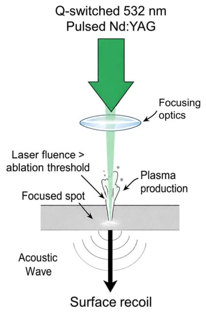
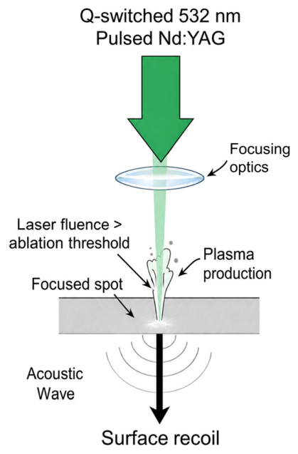
In our system, a Q-switched Nd:YAG laser operating at 532 nm delivered a pulse energy of $\mathrm{E} = 8.3$ mJ to a focused spot with an approximate diameter of 0.7 mm. The corresponding nominal laser fluence was approximately $2.2 \mathrm{J}/\mathrm{c}{\mathrm{m}}^2$, which is comparable to or slightly above the reported ablation threshold [30]. Operation in the ablation regime was further supported by the observation of a small, localized surface mark at the excitation site and a high-amplitude ultrasonic response. Figure 1 illustrates the mechanism of laser-ultrasound generation in the ablation regime. Under ablation conditions, plasma expansion and material ejection produce a transient recoil pressure that launches a broadband acoustic pulse into the specimen. For the through-thickness measurements, the TOF of this acoustic pulse was measured.

Figure 1. Schematic of generating laser ultrasound in the ablation regime.

2.2. Interferometric Detection Using a 3×3 Fiber-Coupler

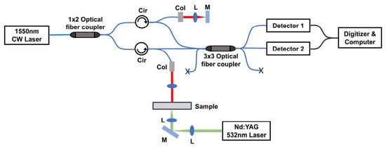
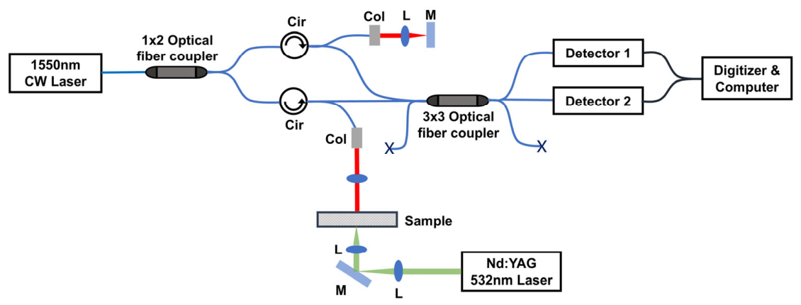
The surface displacements induced by the ultrasonic waves and their subsequent echoes were detected using a fiber-optic interferometer based on a 3×3 fiber coupler, as shown in Figure 2. A continuous-wave (CW) laser operating at a wavelength of 1550 nm was used as the probe source. The system was configured as a passive fiber-optic interferometer to simplify alignment and improve environmental stability.

Figure 2. Schematic of the interferometric detection system based on a 3×3 fiber coupler. A 532 nm Nd:YAG laser pulse generates ultrasound in the sample, while a 1550 nm continuous-wave (CW) laser is used as the interferometric probe source. Cir: circulator; Col: collimator; L: lens; M: mirror.

The probe light was divided into a sensing arm and a reference arm. In the reference arm, a circulator (Cir) directed the optical beam toward a free-space path consisting of a collimator (Col), lens (L), and mirror (M), and routed the reflected reference beam back toward a 3×3 fiber coupler. The collimator and lens conditioned the reference beam, while the mirror provided a controlled reflection for interferometric recombination. A mirror-based reference was used instead of relying on the weak Fresnel reflection made at the bare fiber end to provide a stronger and well-defined reference signal. The sensing beam was directed onto the rear surface of the sample, opposite the excitation side. The surface displacement induced by the propagating ultrasonic waves modulated the optical path length of the sensing arm. The sensing and reference beams were recombined by the 3×3 coupler, producing three interference outputs with intrinsic phase offsets.

In this study, two of the three output channels were acquired and used as inputs to the deep-learning-based demodulator. For an ideal 3×3 coupler, adjacent outputs have a nominal relative phase difference of approximately $2\mathsf{\pi }/3$; therefore, two adjacent outputs provide two non-degenerate phase-shifted interferometric measurements containing sufficient phase diversity for the proposed two-channel NID. The third output can provide additional redundancy and may be beneficial for further noise suppression or self-calibration, but it is not required by the present two-input demodulation framework and was therefore not acquired in this proof-of-concept implementation. In contrast, the two outputs of a conventional 2×2 coupler are nominally complementary, with a relative phase difference of approximately $\mathsf{\pi }$, and do not by themselves provide independent quadrature information. Consequently, an additional phase-shifting or modulation mechanism would generally be required to obtain comparable phase-diverse measurements. The 3×3 coupler was therefore selected because it intrinsically provides passive phase-shifted outputs without requiring active bias control. The displacement-induced phase variation Δϕ(t) is related to the out-of-plane displacement u(t) by:

$$\mathsf{\Delta }\mathsf{\varphi }\left(\mathrm{t}\right)={\displaystyle \frac{4\mathsf{\pi }}{\mathsf{\lambda }}}\mathrm{u}\left(\mathrm{t}\right)$$

(2)

where λ is the wavelength of the probe laser.

The total interferometric phase can be written as

$$\mathsf{\varphi }\left(\mathrm{t}\right)={\mathsf{\varphi }}_0+\mathsf{\Delta }\mathsf{\varphi }\left(\mathrm{t}\right)$$

(3)

where ${\mathsf{\varphi }}_0$ is a static initial phase bias. The two measured intensity signals can be expressed as:

$${\mathrm{I}}_1\left(\mathrm{t}\right) = {\mathrm{A}}_1 + {\mathrm{B}}_1\cos [\mathsf{\varphi }\left(\mathrm{t}\right) + {\mathsf{\delta }}_1]$$

(4)

$${\mathrm{I}}_2\left(\mathrm{t}\right)={\mathrm{A}}_2+{ \mathrm{B}}_2\cos [\mathsf{\varphi }\left(\mathrm{t}\right)+{\mathsf{\delta }}_2]$$

(5)

where ${\mathrm{A}}_1$ and ${\mathrm{A}}_2$ are the DC offsets, ${\mathrm{B}}_1$ and ${\mathrm{B}}_2$ are the AC amplitudes, and ${\mathsf{\delta }}_1$ and ${\mathsf{\delta }}_2$ are the intrinsic phase offsets of the two output channels. In practice, the phase separation may deviate from its ideal value because of coupler imperfections, unequal splitting ratios, photodetector gain mismatch, and environmental perturbations. These nonidealities motivate the use of a learning-based demodulation framework.

2.3. Deep Learning-Based Phase Demodulation

Accurate recovery of the optical phase from the intensity signals measured at the two interferometer output channels is essential for reconstructing the ultrasonic-induced surface displacement. Conventional demodulation methods, including arctangent-based phase retrieval, ellipse fitting, and iterative least-squares approaches, use analytical correction and calibration to improve phase-reconstruction accuracy [31,32,33,34,35,36,37,38,39]. However, these methods generally require several sequential processing steps, including parameter estimation, quadrature compensation, and explicit phase unwrapping. Their performance may deteriorate under low SNR conditions or when the parameters of the interferometric system vary over time.

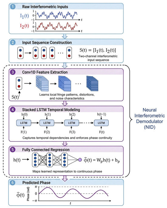
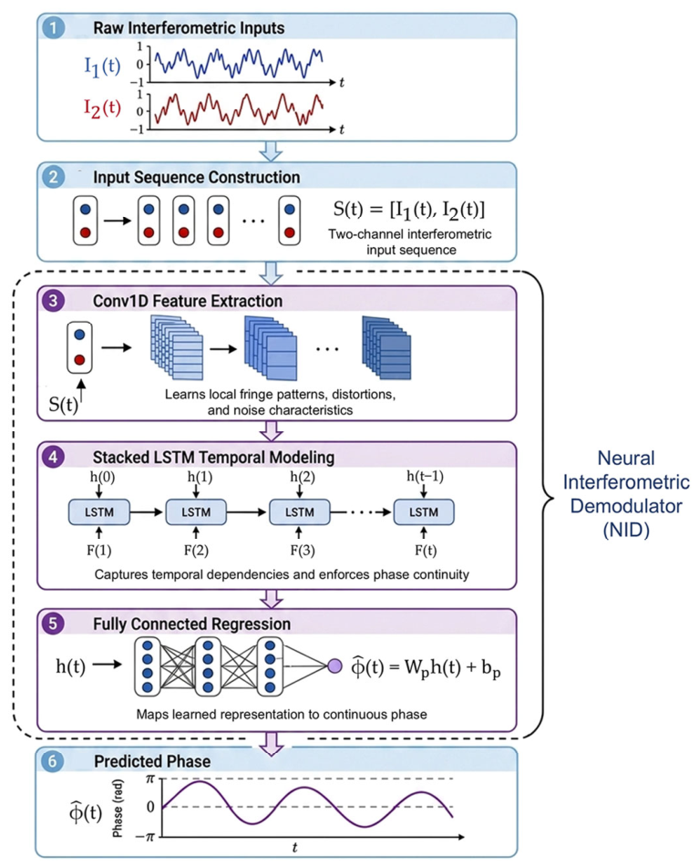
To address these limitations, we propose a neural interferometric demodulator (NID) that learns the nonlinear relationship between the raw interferometric intensity signals and the continuous optical phase. The overall architecture and processing pipeline are presented in Figure 3. The model combines one-dimensional convolutional layers for local temporal-feature extraction with long short-term memory (LSTM) layers for sequence modeling [40,41].

Figure 3. Workflow of the proposed deep learning-based phase demodulation algorithm. Two raw intensity signals ${\mathrm{I}}_1\left(\mathrm{t}\right)$ and ${\mathrm{I}}_2\left(\mathrm{t}\right)$ are combined to form the input sequence $\mathrm{S}\left(\mathrm{t}\right)$, which is processed by the neural interferometric demodulator (NID). The NID consists of Conv1D-based local feature extraction, stacked LSTM layers for temporal modeling, and a fully connected regression layer that maps the learned representation to the predicted continuous optical phase $\widehat{\mathsf{\varphi }}\left(\mathrm{t}\right)$.

Learning-based demodulation has previously been investigated for interferometric fiber-optic sensors based on 3×3 couplers. For example, an LSTM network optimized using an artificial bee colony algorithm was applied to map an interferometric signal to the measured temperature [42]. However, that approach still used a conventional arctangent operation to recover the phase and learned only the subsequent relationship between the recovered phase and the sensing quantity. In contrast, the proposed NID learns the phase-demodulation process itself by mapping the raw two-channel interferometric signals directly to a continuous optical phase sequence. This architecture is intended to reduce sensitivity to noise and fringe distortion while preserving the temporal continuity of the reconstructed phase.

The input sequence at time $\mathrm{t}$ is defined as

$$\mathrm{S}\left(\mathrm{t}\right)={[{\mathrm{I}}_1\left(\mathrm{t}\right), {\mathrm{I}}_2\left(\mathrm{t}\right)]}^{\mathrm{T}}$$

(6)

It is processed by using one-dimensional convolutional layers to extract local temporal features:

$$\mathrm{F}\left(\mathrm{t}\right) = \mathrm{Conv}1\mathrm{D}\left(\mathrm{S}\right(\mathrm{t}\left)\right)$$

(7)

where $\mathrm{F}\left(\mathrm{t}\right)$ denotes the feature vector at time step $\mathrm{t}$. The extracted features represent local fringe structure, amplitude imbalance, waveform distortion, and noise characteristics.

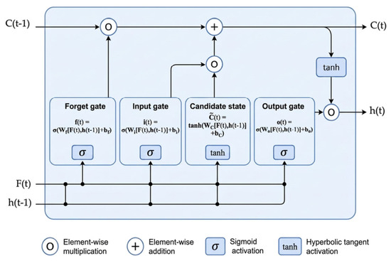
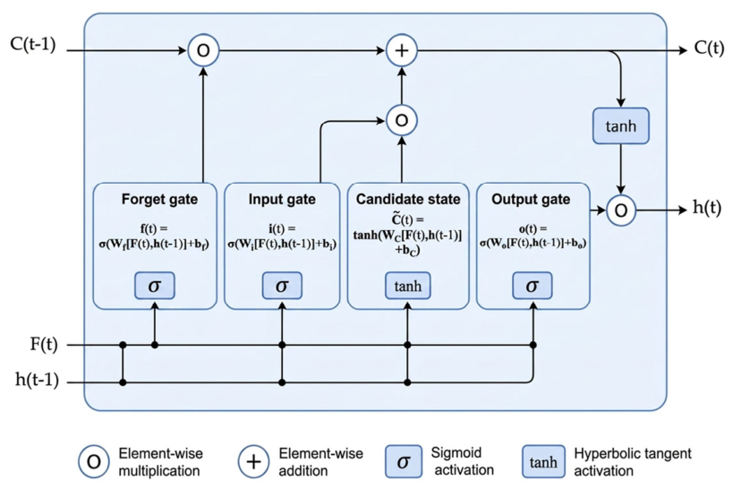
The feature sequence $\mathrm{F}\left(\mathrm{t}\right)$ is then processed by a stacked LSTM network consisting of two layers to model temporal dependencies and enforce smooth phase evolution. The internal structure of the LSTM unit is illustrated in Figure 4. For a given LSTM layer, the hidden-state update at time step $\mathrm{t}$ is governed by:

$$\mathrm{f}\left(\mathrm{t}\right) = \mathsf{\sigma }({\mathrm{W}}_{\mathrm{f}}[\mathrm{F}\left(\mathrm{t}\right),\mathrm{h}(\mathrm{t} - 1)] + {\mathrm{b}}_{\mathrm{f}})$$

(8a)

$$\mathrm{i}\left(\mathrm{t}\right)= \mathsf{\sigma }({\mathrm{W}}_{\mathrm{i}}[\mathrm{F}\left(\mathrm{t}\right),\mathrm{h}(\mathrm{t} - 1)]+{\mathrm{b}}_{\mathrm{i}})$$

(8b)

$$\tilde{\mathrm{C}}\left(\mathrm{t}\right)= \tanh ({\mathrm{W}}_{\mathrm{c}}[\mathrm{F}\left(\mathrm{t}\right),\mathrm{h}(\mathrm{t} - 1)]+{\mathrm{b}}_{\mathrm{c}})$$

(8c)

$$\mathrm{C}\left(\mathrm{t}\right)= \mathrm{f}\left(\mathrm{t}\right) \odot \mathrm{C}(\mathrm{t} - 1)+ \mathrm{i}\left(\mathrm{t}\right) \odot \tilde{\mathrm{C}}\left(\mathrm{t}\right)$$

(8d)

$$\mathrm{o}\left(\mathrm{t}\right)= \mathsf{\sigma }({\mathrm{W}}_{\mathrm{o}}[\mathrm{F}\left(\mathrm{t}\right),\mathrm{h}(\mathrm{t} - 1)]+{\mathrm{b}}_{\mathrm{o}})$$

(8e)

$$\mathrm{h}\left(\mathrm{t}\right)= \mathrm{o}\left(\mathrm{t}\right) \odot \tanh (\mathrm{C}\left(\mathrm{t}\right))$$

(8f)

where f(t), i(t), and o(t) denote the forget, input, and output gates, respectively; $\tilde{\mathrm{C}}\left(\mathrm{t}\right)$ is the candidate cell state; C(t) is the cell state; h(t) is the hidden state. The matrices ${\mathrm{W}}_{\mathrm{f}}$, ${\mathrm{W}}_{\mathrm{i}}$, ${\mathrm{W}}_{\mathrm{c}}$, and ${\mathrm{W}}_{\mathrm{o}}$ are trainable weight matrices, while ${\mathrm{b}}_{\mathrm{f}}$, ${\mathrm{b}}_{\mathrm{i}}$, ${\mathrm{b}}_{\mathrm{c}}$, and ${\mathrm{b}}_{\mathrm{o}}$ are corresponding bias vectors. The function σ(⋅) denotes the sigmoid activation function, $\tan \mathrm{h}(\cdot )$ denotes the hyperbolic tangent activation function; and $\odot$ denotes element-wise multiplication. By modeling both short- and long-range temporal dependencies, the LSTM layers help reduce noise-induced fluctuations while maintaining continuity in the reconstructed phase sequence.

Figure 4. Internal structure of an LSTM unit used in the proposed NID. At each time step, the Conv1D-extracted feature $\mathrm{F}\left(\mathrm{t}\right)$ and the previous hidden state $\mathrm{h}(\mathrm{t} - 1)$ are used to compute the forget, input, candidate-state, and output gates. These gated operations update the cell state $\mathrm{C}\left(\mathrm{t}\right)$ and produce the hidden state $\mathrm{h}\left(\mathrm{t}\right)$, enabling temporal modeling of the interferometric feature sequence while preserving the phase continuity.

The final fully connected layer maps the LSTM hidden representation to the predicted phase:

$$\widehat{\mathsf{\varphi }}\left(\mathrm{t}\right) = {\mathrm{W}}_{\mathrm{p}}\mathrm{h}\left(\mathrm{t}\right) + {\mathrm{b}}_{\mathrm{p}}$$

(9)

where ${\mathrm{W}}_{\mathrm{p}}$ and ${\mathrm{b}}_{\mathrm{p}}$ are trainable output-layer parameters. The network is trained using the mean squared error (MSE) loss between the predicted phase and the reference phase:

$$\mathrm{L} = {\displaystyle \frac{1}{\mathrm{NT}}}{\displaystyle {\sum }_{\mathrm{n}=1}^{\mathrm{N}}}{\displaystyle {\sum }_{\mathrm{t}=1}^{\mathrm{T}}}{({\widehat{\mathsf{\varphi }}}_{\mathrm{n}}\left(\mathrm{t}\right)-{\mathsf{\varphi }}_{\mathrm{n}}\left(\mathrm{t}\right))}^2$$

(10)

where N is the number of training sequences, T is the number of time samples in each sequence, ${\widehat{\mathsf{\varphi }}}_{\mathrm{n}}\left(\mathrm{t}\right)$ is the predicted phase, and ${\mathsf{\varphi }}_{\mathrm{n}}\left(\mathrm{t}\right)$ is the corresponding reference phase obtained from calibrated measurements. Because the NID is trained using experimental interferometric data, it can learn to compensate for gain mismatch, DC offsets, deviations from the ideal phase separation, and other system-specific interferometric distortions represented in the training dataset.

3. Results and Discussion

3.1. Experimental Setup

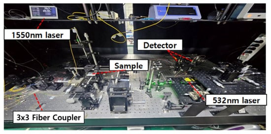
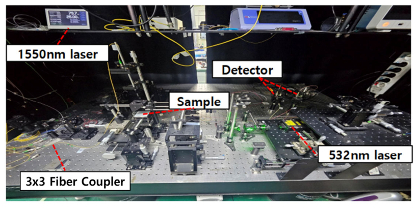
A photograph of the laboratory setup is shown in Figure 5. Ultrasonic waves were generated using a pulsed laser operating at a wavelength of 532 nm. The laser beam was focused to a spot diameter of approximately 0.7 mm. The measured pulse energy at the sample surface was 8.3 mJ, corresponding to a nominal fluence of approximately $2.2 \mathrm{J}/\mathrm{c}{\mathrm{m}}^2$. The resulting rear-surface displacement was detected on the opposite side of the specimen using a 1550 nm CW laser as the interferometric probe source.

Figure 5. Photograph of the laboratory setup for fully non-contact thickness measurement. The main components include a 532 nm pulsed excitation laser, a 1550 nm continuous-wave probe laser, an aluminum plate, a 3×3 fiber coupler, and photodetectors for signal acquisition.

Flat aluminum plates with nominal thicknesses of 2, 6, and 10 mm were used as specimens. The material properties of the aluminum specimens are summarized in Table 1. The TOF of the acoustic pulse was used to estimate the plate thickness. The two interferometric output signals were digitized at a sampling rate of 500 MS/s. Each acquisition contained 2080 time samples, corresponding to a record length of 4.16 µs.

Table 1. Material properties of the aluminum specimens used in this study.

Property	Value
Density	2700 kg/m3
Acoustic speed	6350 m/s
Shear wave speed	3150 m/s
Rayleigh wave speed	2940 m/s
Thermal expansion coefficient	2.31 × 10−5 K−1
Melting point	934 K
Boiling point	2790 K

3.2. Training and Reference-Phase Generation

The proposed NID was trained using data acquired from the 3×3 fiber-coupler interferometer. The training dataset included controlled interferometric measurements and representative laser-ultrasonic signals acquired under different signal conditions, spanning both sub-2π phase excursions and multi-fringe phase variations exceeding 2π. For supervised learning, reference phase trajectories were generated by constructing Lissajous curves from the two-channel signals, ${\mathrm{I}}_1\left(\mathrm{t}\right)$ and ${\mathrm{I}}_2\left(\mathrm{t}\right)$, and applying ellipse fitting. The fitted ellipse parameters, including the DC offsets, AC amplitudes, and intrinsic phase difference, were used to reconstruct the wrapped phase, which was subsequently unwrapped to obtain a continuous reference phase. To suppress random noise and improve the quality of the reference labels, the extracted phase traces were baseline-corrected using the pre-trigger interval and then coherently averaged.

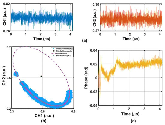
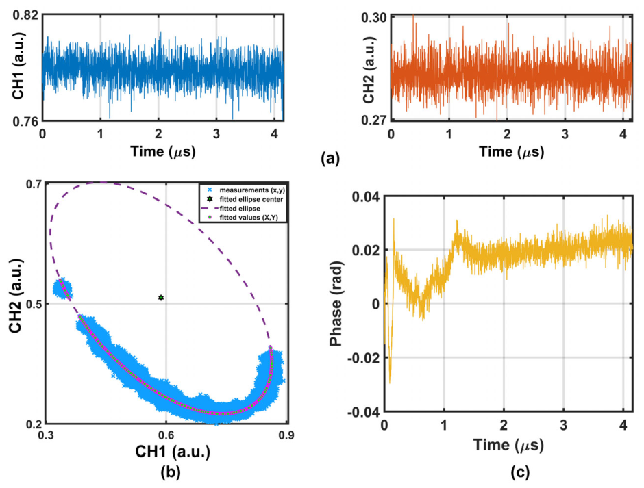
Figure 6 presents a representative example of the reference-label generation procedure, including the interferometric intensity signals in Figure 6a, the fitted Lissajous curve in Figure 6b, and the corresponding reference phase in Figure 6c. A single excitation pulse generated a series of echo signals with a duration of approximately $4 \mathsf{\mu }\mathrm{s}$ in each output channel. Because the phase excursion within a single acquisition covered only a limited portion of the interference cycle owing to the small amplitude of the ultrasonic-induced displacement, the corresponding Lissajous curve formed a compact, diffuse cluster rather than a complete ellipse. However, repeated measurements acquired under the same experimental conditions exhibited slow phase-bias drift, causing the clusters to shift along the underlying elliptical trajectory. The ellipse parameters could therefore be estimated from the combined repeated measurements and subsequently used to extract the phase variation from each individual interferometric acquisition. The reference phase was then obtained by coherently averaging the extracted phase traces.

Figure 6. Representative example of the reference-label generation procedure used for NID training. (a) Raw interferometer output signals I₁(t) (CH1) and I₂(t) (CH2) acquired with a single excitation laser pulse. (b) Combined Lissajous curve constructed from repeated measurements of the two channels; the dotted line indicates the fitted ellipse. (c) Reference phase reconstructed using the fitted ellipse parameters.

It should be noted that the reference phase obtained from ellipse fitting represents a calibrated reference rather than an error-free ground truth. Errors in the estimated ellipse parameters, including the DC offsets, signal amplitudes, and intrinsic phase difference, may introduce deviations into the reconstructed reference phase. Noise and incomplete sampling of the Lissajous curve may further affect the reference labels. Because the NID is trained using supervised regression, systematic errors consistently present in these labels may propagate into the learned phase reconstruction. To reduce random labeling errors, the ellipse parameters were estimated from combined repeated measurements that sampled a broader portion of the underlying Lissajous curve, and the reconstructed reference phases were subsequently baseline-corrected and coherently averaged. Nevertheless, the ultimate accuracy of the NID remains dependent on the quality of the reference phase used during training.

Ellipse fitting was used only to generate the reference labels for network training and was not a part of the NID inference pipeline. Before training, the input signals were normalized, and the dataset was divided into training and validation subsets. The network was trained using the MSE loss defined in Equation (10). After training, the NID was applied without retraining or sample-specific parameter adjustment.

3.3. NID Phase Reconstruction and Validation

3.3.1. PZT-Based Phase-Demodulation Validation

The phase-demodulation performance of the proposed NID was evaluated using PZT-modulated calibration measurements acquired at static chamber pressures of 10, 15, 20, and 25 kPa. For each pressure condition, a PZT continuously displaced the reference mirror, thereby generating time-varying interferometric signals with phase excursions extending across multiple interference fringes. The chamber pressure was adjusted between acquisitions and remained constant during each measurement. Variations in chamber pressure modified the optical condition of the sensing arm and therefore provided distinct interferometric operating conditions for evaluating the phase-demodulation performance.

The PZT calibration measurements differ intentionally from the laser-ultrasonic measurements in both temporal scale and modulation depth. The PZT produces a controlled, relatively slow displacement of the reference mirror over a millisecond-scale interval, allowing the interferometric phase to traverse multiple fringe periods and thereby providing a suitable dataset for evaluating phase reconstruction across 2π wrapping boundaries. In contrast, laser-ultrasonic excitation generates a short-duration transient response associated with acoustic-wave propagation through the aluminum plate, resulting in microsecond-scale signals with substantially smaller phase excursions. Thus, the PZT measurements are used primarily to validate the phase-demodulation capability of the NID over a broad phase range, whereas the aluminum measurements evaluate its application to weak, rapidly varying laser-ultrasonic signals for thickness estimation.

For benchmarking, a calibrated reference phase was generated from the measured ${\mathrm{I}}_1\left(\mathrm{t}\right)$ and ${\mathrm{I}}_2\left(\mathrm{t}\right)$ signals using the ellipse-fitting procedure. The estimated DC offsets, fringe amplitudes, and intrinsic phase difference were used to reconstruct the wrapped phase, which was subsequently unwrapped to obtain the continuous reference phase. The proposed NID received only the paired raw interferometric signals as input and directly predicted the corresponding continuous phase during inference.

The NID was compared with the conventional 3×3 standard ellipse-fitting (3×3-SEF) method [33]. In the present implementation, 3×3-SEF was applied using the same signals, ${\mathrm{I}}_1\left(\mathrm{t}\right)$ and ${\mathrm{I}}_2\left(\mathrm{t}\right)$. The optional laser-intensity normalization requiring an additional monitor channel was not used. The 3×3-SEF method estimates the ellipse parameters from the interferometric measurements, compensates for the channel imbalance, and subsequently reconstructs the optical phase through analytical quadrature processing.

Phase-reconstruction performance was quantified using the root mean squared error (RMSE), mean absolute error (MAE), normalized cross-correlation (NCC), and signal-to-error ratio (SER) with respect to the calibrated reference phase. For a phase sequence containing (${\mathrm{N}}_{\mathrm{s}}$) samples, the phase RMSE was calculated as

$$\mathrm{RMSE}=\sqrt{{\displaystyle \frac{1}{{\mathrm{N}}_{\mathrm{s}}}}{\displaystyle {\sum }_{\mathrm{t}=1}^{{\mathrm{N}}_{\mathrm{s}}}}{(\widehat{\mathsf{\varphi }}\left(\mathrm{t}\right) -\mathsf{\varphi }\left(\mathrm{t}\right))}^2}$$

(11)

and the MAE was calculated as

$$\mathrm{MAE}={\displaystyle \frac{1}{{\mathrm{N}}_{\mathrm{s}}}}{\sum }_{\mathrm{t}=1}^{{\mathrm{N}}_{\mathrm{s}}}\left|\widehat{\mathsf{\varphi }}\left(\mathrm{t}\right)-\mathsf{\varphi }\left(\mathrm{t}\right)\right|.$$

(12)

The NCC was used to assess preservation of the temporal phase waveform:

$$\mathrm{NCC} = {\displaystyle \frac{{\displaystyle {\sum }_{\mathrm{t}=1}^{{\mathrm{N}}_{\mathrm{s}}}}(\widehat{\mathsf{\varphi }}\left(\mathrm{t}\right)-\overline{\widehat{\mathsf{\varphi }}}\left)\right(\mathsf{\varphi }\left(\mathrm{t}\right)-\stackrel{\mathrm{-}}{\mathsf{\varphi }})}{\sqrt{{\displaystyle {\sum }_{\mathrm{t}=1}^{{\mathrm{N}}_{\mathrm{s}}}}{(\widehat{\mathsf{\varphi }}\left(\mathrm{t}\right)-\overline{\widehat{\mathsf{\varphi }}})}^2}\sqrt{{\displaystyle {\sum }_{\mathrm{t}=1}^{{\mathrm{N}}_{\mathrm{s}}}}{(\mathsf{\varphi }\left(\mathrm{t}\right)-\stackrel{\mathrm{-}}{\mathsf{\varphi }})}^2}}}$$

(13)

where $\overline{\widehat{\mathsf{\varphi }}}$ and $\stackrel{\mathrm{-}}{\mathsf{\varphi }}$ denote the temporal means of the reconstructed and reference phases, respectively. The phase SER was defined as

$$\mathrm{SER}={10\log }_{10}\left({\displaystyle \frac{{\displaystyle {\sum }_{\mathrm{t}=1}^{{\mathrm{N}}_{\mathrm{s}}}}{\mathsf{\varphi }}^2\left(\mathrm{t}\right)}{{\displaystyle {\sum }_{\mathrm{t}=1}^{{\mathrm{N}}_{\mathrm{s}}}}{(\mathsf{\varphi }\left(\mathrm{t}\right)-\widehat{\mathsf{\varphi }}\left(\mathrm{t}\right))}^2}}\right).$$

(14)

Together, these metrics quantify the absolute reconstruction error, waveform agreement, and relative magnitude of the residual phase error.

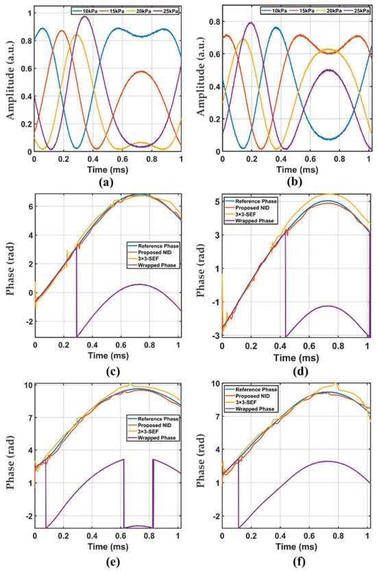
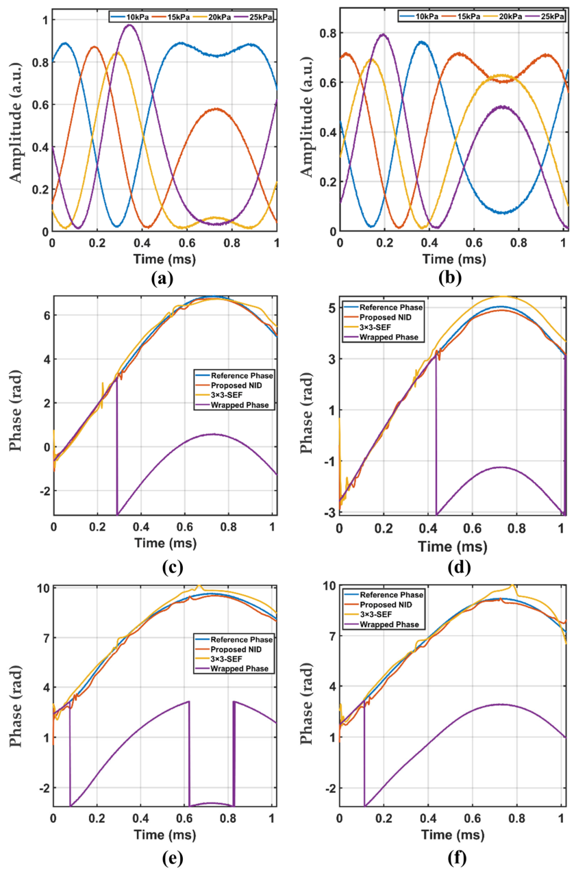
Figure 7 presents representative phase-demodulation results obtained at chamber pressures of 10, 15, 20, and 25 kPa. Figure 7a,b show the corresponding raw interferometric signals ${\mathrm{I}}_1\left(\mathrm{t}\right)$ and ${\mathrm{I}}_2\left(\mathrm{t}\right)$, while Figure 7c–f compare the calibrated reference phase, the proposed NID result, the 3×3-SEF result, and the wrapped phase for the 4 operating conditions. Across all pressure conditions, the NID closely follows the calibrated continuous reference phase. The 3×3-SEF method reproduces the general phase evolution but exhibits larger localized deviations and residual fluctuations, particularly where the interferometric trajectory is affected by amplitude imbalance or waveform distortion.

Figure 7. Quantitative phase-demodulation validation made using PZT-modulated interferometric measurements. (a) Channel-1 signal ${\mathrm{I}}_1\left(\mathrm{t}\right)$ and (b) channel-2 signal ${\mathrm{I}}_2\left(\mathrm{t}\right)$ acquired at chamber pressures of 10, 15, 20, and 25 kPa. (c–f) Phase reconstruction at 10, 15, 20, and 25 kPa, respectively, comparing the calibrated reference phase, proposed NID, conventional 3×3-SEF method, and wrapped phase.

Importantly, the PZT measurements produce phase excursions extending beyond 2π, and the wrapped phase shown in Figure 7c–f therefore contains distinct 2π discontinuities. In contrast, the NID reconstructs a continuous phase trajectory across these wrapping boundaries without applying a separate phase-unwrapping algorithm during inference. This experiment provides direct validation of the continuity of the NID output across phase-wrapping boundaries. It should be emphasized, however, that phase unwrapping is used during generation of the calibrated reference labels; therefore, the present result demonstrates elimination of a separate phase-unwrapping operation specifically from the NID inference pipeline rather than from the overall training and calibration procedure.

The quantitative comparison is summarized in Table 2. At 10 kPa, the phase RMSE decreases from 0.048 rad for 3×3-SEF to 0.029 rad for the proposed NID, while the NCC increases from 0.983 to 0.996. Similar improvements are observed at other pressure conditions. At 25 kPa, the NID achieves an RMSE of 0.041 rad, compared with 0.071 rad for 3×3-SEF, while maintaining an NCC of 0.997. The NID also consistently provides lower MAE and higher SER across all 4 operating conditions. These results demonstrate improved agreement with the calibrated reference phase and more consistent phase reconstruction across the investigated interferometric operating conditions.

Table 2. Quantitative phase demodulation performance at different chamber pressure levels.

Pressure	Method	RMSE (rad)	MAE (rad)	SER (dB)	NCC
10 kPa	3×3-SEF Proposed NID	0.048 0.029	0.039 0.023	28.5 32.2	0.983 0.996
15 kPa	3×3-SEF Proposed NID	0.052 0.033	0.045 0.024	26.7 34.1	0.982 0.997
20 kPa	3×3-SEF Proposed NID	0.063 0.038	0.058 0.031	24.9 34.6	0.980 0.998
25 kPa	3×3-SEF Proposed NID	0.071 0.041	0.064 0.035	23.4 34.9	0.975 0.997

The computational performance of the NID was also compared with the conventional 3×3-SEF method using two-channel input sequences of 2 × 1024 samples. The measured processing time included the complete demodulation procedure for each method; for 3×3-SEF, this comprised Lissajous-curve fitting, phase calculation, and phase unwrapping. The NID required an average processing time of 295 ± 30 μs per sequence, compared with 481 ± 22 μs per sequence for 3×3-SEF, corresponding to an approximately 38.7% reduction in processing time. The corresponding throughputs were approximately 3390 sequences/s for the NID and 2080 sequences/s for 3×3-SEF. These results indicate that, once trained, the NID provides faster phase reconstruction because it directly maps the paired interferometric signals to a continuous phase sequence without requiring the sequential analytical fitting and phase-processing steps used in conventional demodulation. Importantly, the PZT sequences used for the quantitative comparisons presented in Figure 7 and Table 2 were held out from network training and were not used to update the NID parameters.

3.3.2. Aluminum-Plate Phase Reconstruction

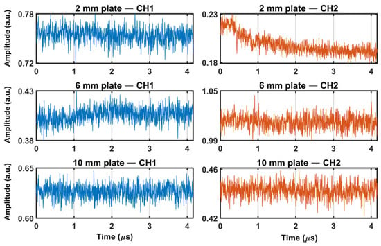
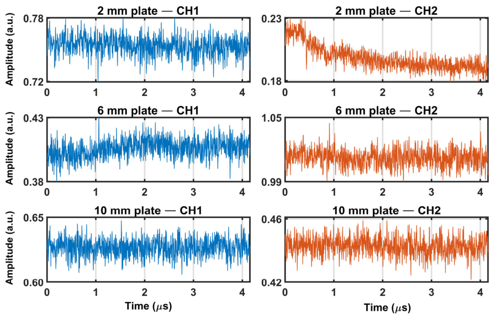
Following the quantitative PZT-based validation, the trained NID was applied to the laser-ultrasonic measurements of the aluminum plates. The two interferometric output signals, ${\mathrm{I}}_1\left(\mathrm{t}\right)$ and ${\mathrm{I}}_2\left(\mathrm{t}\right)$, were acquired at a sampling rate of 500 MS/s. Representative raw interferometric signals acquired from the two output channels for the 2, 6, and 10 mm aluminum plates are shown in Figure 8. These signals represent the experimental inputs supplied directly to the trained NID and therefore provide a direct link between the two-channel interferometric acquisition and the subsequent phase reconstruction. The paired channels exhibit time-dependent intensity variations produced by ultrasonic-induced optical path length modulation in the sensing-arm and reflect the intrinsic phase-offset relationship between the two 3×3-coupler outputs.

Figure 8. Representative raw interferometric signals acquired from two output ports of the 3×3 interferometer following a single excitation pulse for 2, 6, and 10 mm aluminum plates. The left and right columns correspond to CH1 (I₁(t)) and CH2 (I₂(t)), respectively. These paired signals constitute the experimental inputs supplied directly to the trained NID for optical phase reconstruction.

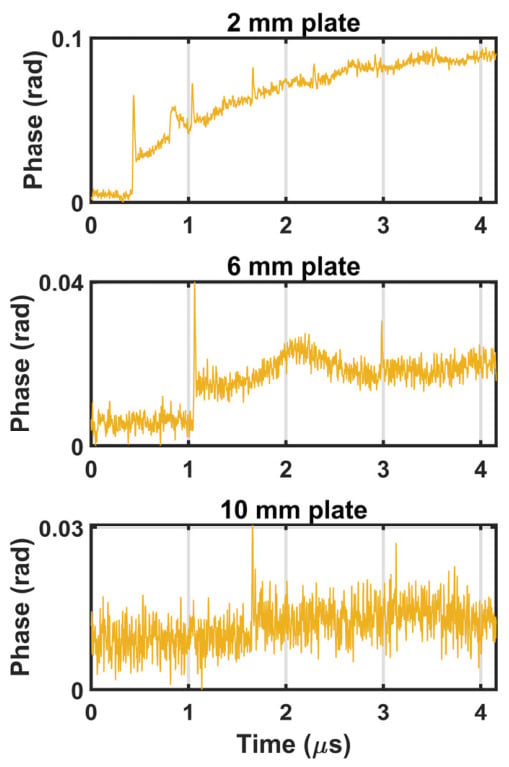
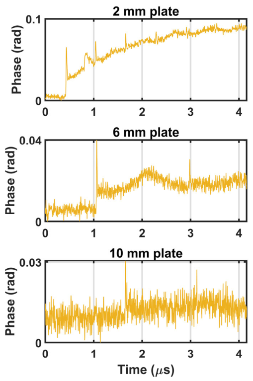
For each acquisition, the NID mapped the two-channel input directly to the corresponding continuous optical phase, $\widehat{\mathsf{\varphi }}\left(\mathrm{t}\right)$. To improve phase stability and reduce random noise, each reconstructed phase trace was baseline-corrected using the pre-trigger interval, and 50 NID-reconstructed phase traces acquired under identical measurement conditions were coherently averaged. The resulting phase signals are shown in Figure 9.

Figure 9. Coherently averaged optical phase $\widehat{\mathsf{\varphi }}\left(\mathrm{t}\right)$ reconstructed by the trained NID directly from the paired interferometric signals, for the three aluminum plate thicknesses.

The reconstructed aluminum-plate phase signals exhibit distinct ultrasonic-induced temporal features associated with acoustic-wave propagation through the specimens. The time interval between consecutive acoustic-wave arrival features increases with plate thickness, while the multiple features observed for the 2 mm plate arise from repeated back-and-forth reflections of the acoustic wave within the plate. Unlike the PZT validation measurements in Figure 7, phase excursions produced by the LUS with aluminum remain well below 2π. Accordingly, the aluminum measurements are used to demonstrate the application of the NID to weak LUS signals and subsequent thickness estimation, whereas the PZT measurements provide the direct experimental validation of continuous phase reconstruction across multiple phase-wrapping boundaries.

3.4. Displacement Reconstruction and Time-of-Flight (TOF) Estimation

After phase reconstruction, the phase predicted by the NID, $\widehat{\mathsf{\varphi }}\left(\mathrm{t}\right)$, was baseline-corrected using the pre-trigger interval to obtain the displacement-induced phase variation, $\mathsf{\Delta }\widehat{\mathsf{\varphi }}\left(\mathrm{t}\right)$. This phase variation was then converted into surface displacement using Equation (2). Because the detection was performed in reflection geometry, the reconstructed rear-surface displacement is given by

$$\mathrm{u}\left(\mathrm{t}\right)={\displaystyle \frac{\mathsf{\lambda }}{4\mathsf{\pi }}}\mathsf{\Delta }\widehat{\mathsf{\varphi }}\left(\mathrm{t}\right).$$

(15)

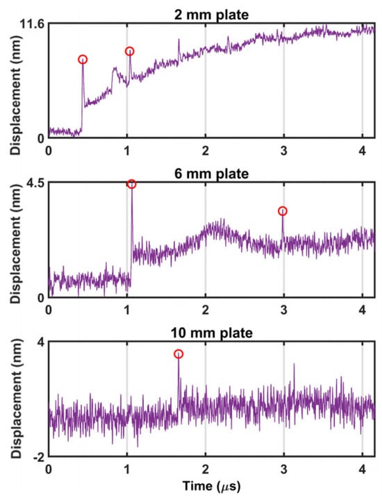
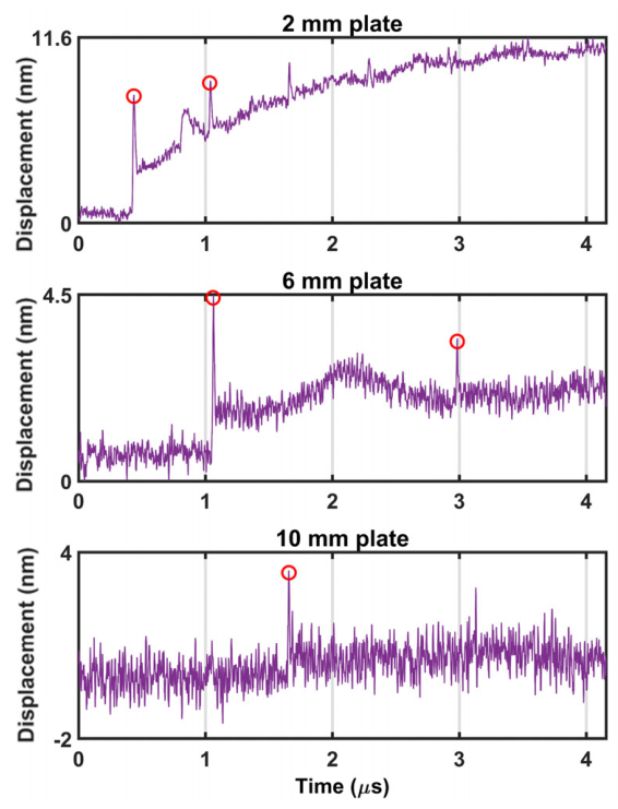
The time-varying displacement waveforms reconstructed from the coherently averaged NID phase signals are shown in Figure 10 for the three aluminum plates. The reconstructed waveforms exhibit distinct peaks associated with the arrival of ultrasonic pulses. The TOF was determined by identifying the selected arrival features in the displacement waveforms. In general, the plate thickness can be estimated either from the one-way flight time or from the time interval between two consecutive acoustic-wave arrivals resulting from repeated back-and-forth propagation and reflection between the two surfaces of the plate.

Figure 10. The displacement reconstructed from the coherently averaged NID phase. The displacement was obtained using Eq. (15) with $\mathsf{\lambda } = 1550$ nm. Red circles indicate the selected TOF features used for the thickness estimation: two consecutive longitudinal-wave arrivals at the detection surface for the 2 mm and 6 mm plates, and the first arrival for the 10 mm plate.

When the first arrival is clearly resolved, the one-way flight time is defined as ${ \mathrm{t}}_{\mathrm{L}}= {\mathrm{t}}_1 -{\mathrm{t}}_0$, where ${\mathrm{t}}_1$ is the measured first-arrival time and ${\mathrm{t}}_0$ is the time-origin offset between laser excitation and data acquisition. In the present analysis, ${\mathrm{t}}_0$ was assumed to be zero according to the acquisition trigger. However, the residual uncertainty in ${\mathrm{t}}_0$ was not independently characterized. The plate thickness can then be calculated as

$$\mathrm{d}={\mathrm{c}}_{\mathrm{L}}{\mathrm{t}}_{\mathrm{L}}$$

(16)

where $\mathrm{d}$ is the plate thickness, ${\mathrm{c}}_{\mathrm{L}}$ is the acoustic velocity in aluminum, and ${\mathrm{t}}_{\mathrm{L}}$ is the one-way flight time.

Alternatively, when two consecutive acoustic-wave arrivals at the detection surface are clearly identifiable, the echo interval is defined as $\mathsf{\Delta }\mathrm{t} = {\mathrm{t}}_2-{\mathrm{t}}_1$, where ${\mathrm{t}}_1$ and ${\mathrm{t}}_2$ are the measured first- and second-arrival times, respectively. Because both arrival times are referenced to the same time origin, the offset ${\mathrm{t}}_0$ cancels. The plate thickness can therefore be estimated as

$$\mathrm{d}={\mathrm{c}}_{\mathrm{L}}\mathsf{\Delta }\mathrm{t}/2.$$

(17)

In this study, the TOF-estimation method was selected according to the most reliable arrival features available in each reconstructed displacement waveform. For the 2 and 6 mm plates, two consecutive acoustic-wave arrivals at the detection surface were clearly observed; therefore, the echo-interval method in Equation (17) was used. This method is advantageous because it depends only on the time difference between successive arrivals and is therefore less sensitive to the uncertainty in the absolute excitation time. For the 10 mm plate, the expected second arrival occurred outside the acquisition window; therefore, the first-arrival method in Equation (16) was used.

The measured arrival times and echo intervals are summarized in Table 3. Using an acoustic velocity of ${\mathrm{c}}_{\mathrm{L}} = 6350 \mathrm{m}/\mathrm{s}$, the TOF-based thicknesses were calculated and compared with reference measurements obtained using a vernier caliper, as summarized in Table 4. The estimated thicknesses were $1.911 \text{±} 0.024$ mm, $6.102 \pm 0.070$ mm, and $10.516$ mm with a partial standard uncertainty of 0.127 mm for the nominally 2, 6, and 10 mm plates, respectively. These values correspond to errors of $-0.096$ mm, $-0.001$ mm, and $0.506$ mm and relative errors of $-4.78\%$, $-0.02\%$, and $5.05\%$, respectively.

Table 3. Measured acoustic pulse arrival times and the echo intervals for the three aluminum plates.

Nominal Thickness (mm)	First Arrival t1 (µs)	Second Arrival t2 (µs)	Interval Δt = t2 − t1 (µs)
2	0.436	1.038	0.602
6	1.062	2.984	1.922
10	1.656	-	-

Table 4. TOF-based thickness estimates with measurement uncertainty and comparison with caliper reference measurements.

Plate (mm)	Method	Caliper Reference (mm)	Estimated Thickness d ± u(d) (mm)	Error (mm)	Relative Error (%)
2	Echo-interval	2.007	1.911 ± 0.024	−0.096	−4.78
6	Echo-interval	6.103	6.102 ± 0.070	−0.001	−0.02
10	First-arrival	10.010	10.516 ± 0.127	0.506	5.05

The estimated thickness of the 6 mm plate showed excellent agreement with the caliper reference measurement. The larger relative deviation observed for the 2 mm plate can be attributed partly to its shorter echo interval, for which a small timing deviation produces a larger fractional thickness error. For the 10 mm plate, the larger error was associated with the use of the first-arrival method because the second acoustic-wave arrival occurred outside the acquisition window.

The TOF-based thickness estimate depends on several measurement parameters. For the first-arrival method, $\mathrm{d} = {\mathrm{c}}_{\mathrm{L}}({\mathrm{t}}_1 -{\mathrm{t}}_0)$, and therefore residual trigger-synchronization or time-origin errors directly affect the estimated thickness. Similarly, uncertainty or systematic bias in identifying the first-arrival time ${\mathrm{t}}_1$, arising from waveform shape, noise, or arrival-feature localization, propagates directly into the thickness estimate. In contrast, for the echo-interval method, the common time-origin offset cancels when $\mathsf{\Delta }\mathrm{t} = {\mathrm{t}}_2-{\mathrm{t}}_1$ is calculated, reducing sensitivity to trigger synchronization. The estimated thickness is also directly proportional to the assumed acoustic velocity ${\mathrm{c}}_{\mathrm{L}}$; consequently, any deviation of the actual specimen velocity from the adopted value of 6350 m/s produces a proportional thickness bias. Such deviations may arise from specimen-specific alloy composition, temperature, or material condition. For the 10 mm plate, the second acoustic-wave arrival occurred outside the acquisition window, necessitating use of the first-arrival method. The observed error should therefore be interpreted primarily as sensitivity to absolute timing, arrival-feature localization, and the assumed wave velocity rather than as an intrinsic thickness-dependent bias of the first-arrival method.

To quantify the uncertainty in the estimated thickness, u(d), an uncertainty budget was constructed using the experimentally quantified timing contribution and the assumed acoustic velocity uncertainty. For the first-arrival method, the possible contribution of the absolute time origin was also considered theoretically, although it could not be independently quantified in the present experiment. For the echo-interval method, the standard uncertainty in thickness was estimated as

$$\mathrm{u}\left(\mathrm{d}\right)=\sqrt{{[{\displaystyle \frac{{\mathrm{c}}_{\mathrm{L}}}{2}}\mathrm{u}(∆\mathrm{t})]}^2+{[{\displaystyle \frac{∆\mathrm{t}}{2}}\mathrm{u}({\mathrm{c}}_{\mathrm{L}}\left)\right]}^2}$$

(18)

For the first-arrival method, the standard uncertainty was estimated as

$$\mathrm{u}\left(\mathrm{d}\right)=\sqrt{{[{\mathrm{c}}_{\mathrm{L}}\mathrm{u}({\mathrm{t}}_1\left)\right]}^2+{\left[\right({\mathrm{t}}_1-{\mathrm{t}}_0)\mathrm{u}({\mathrm{c}}_{\mathrm{L}}\left)\right]}^2+{[{\mathrm{c}}_{\mathrm{L}}\mathrm{u}({\mathrm{t}}_0\left)\right]}^2}.$$

(19)

The resulting uncertainty contributions are summarized in Table 5. The timing term represents the standard uncertainty associated with determining the selected echo interval $\mathsf{\Delta }\mathrm{t}$ or the measured first-arrival time ${\mathrm{t}}_1$ from repeated measurements. The velocity term assumes a relative standard uncertainty of 1% in the acoustic velocity, ${\mathrm{c}}_{\mathrm{L}} = 6350 \mathrm{m}/\mathrm{s}$. For the echo-interval method, the common time-origin offset cancels when $\mathsf{\Delta }\mathrm{t} = {\mathrm{t}}_2 - {\mathrm{t}}_1$ is calculated. For the first-arrival method used for the 10 mm plate, the residual uncertainty in the absolute time origin was not independently characterized and was therefore not included in the numerical uncertainty budget. Consequently, the combined uncertainty reported for the 10 mm plate represents a partial standard uncertainty based only on first-arrival localization and acoustic velocity uncertainty.

Table 5. Quantified standard-uncertainty contributions for the ultrasonic thickness measurements.

Plate (mm)	Timing Contribution (mm)	Velocity, 1% (mm)	Combined u(d) (mm)
2	0.014	0.019	0.024
6	0.034	0.061	0.070
10	0.071	0.105	0.127 *

* Partial standard uncertainty excluding the unquantified absolute time-origin contribution.

The uncertainty budget shows that the 2 and 6 mm measurements were mainly limited by the assumed uncertainty in ${\mathrm{c}}_{\mathrm{L}}$. For the 10 mm plate, the reported partial uncertainty includes only first-arrival localization and velocity contributions. The uncertainty budget represents the quantified standard-uncertainty contributions and does not capture all possible systematic biases. For the 2 mm plate, the measured error of −0.096 mm is approximately four times the combined standard uncertainty of 0.024 mm. Although the echo-interval method cancels the common time-origin offset, the relatively short echo interval makes the estimated thickness more sensitive to systematic bias in locating the first and second acoustic-wave arrival features. In addition, specimen-specific deviations of the actual acoustic velocity from the assumed value of 6350 m/s may contribute to the observed discrepancy. For the 10 mm plate, the error of 0.506 mm is also approximately four times the reported partial standard uncertainty of 0.127 mm. Because this measurement relies on the first-arrival method, residual trigger synchronization, absolute time-origin uncertainty, and first-arrival localization can directly bias the estimated thickness.

The absolute time-origin uncertainty was not independently characterized and is therefore not included in the numerical budget. Accordingly, the reported uncertainty values should be interpreted as quantified standard uncertainties rather than as a complete representation of all systematic measurement errors.

The NID-derived displacement waveforms provided sufficiently distinct ultrasonic-pulse arrival features for TOF extraction. Because the NID reconstructed a continuous phase trajectory before displacement conversion, the resulting displacement waveforms contained distinguishable arrival features suitable for thickness estimation.

Short-term repeatability was further evaluated using 100 individual acquisitions obtained under unchanged experimental conditions for each aluminum specimen. For the 2 and 6 mm plates, repeatability was assessed from the echo interval, $\mathsf{\Delta }\mathrm{t} ={ \mathrm{t}}_2 -{\mathrm{t}}_1$, whereas the first-arrival time, ${\mathrm{t}}_1$, was used for the 10 mm plate because the second arrival occurred outside the acquisition window. The mean TOF features were 0.607, 1.921, and 1.654 µs for the nominal 2, 6, and 10 mm plates, respectively, with corresponding standard deviations of 0.0046, 0.0093, and 0.0114 µs. These results indicate stable short-term localization of the selected TOF features under unchanged experimental conditions and provide an experimental measure of the repeatability of the thickness-estimation procedure.

Several limitations should be noted. First, the experiments were conducted in the ablation regime to generate strong and broadband ultrasonic waves. Although this improved the signal amplitude, it also produced localized surface modification at the excitation site. Future work should evaluate the proposed demodulation approach under thermoelastic excitation for fully nondestructive inspection. Second, although the added PZT measurements provide additional validation of the phase-demodulation performance under multiple interferometric operating conditions, the thickness-measurement experiments were limited to three aluminum plates with nominal thicknesses of 2, 6, and 10 mm under controlled laboratory conditions. Therefore, the present results should not be interpreted as demonstrating generalization across different materials or various measurement environments. Broader validation using additional metallic materials, thickness ranges, alloy grades, and surface conditions, including rough, coated, or oxidized surfaces, will be required to assess practical generalizability. Future work will also investigate controlled external disturbances, such as mechanical vibration and optical-path perturbations, together with systematic SNR-dependent measurements to quantify the robustness of the complete measurement system. Third, the current TOF-estimation procedure relies on identifiable peak features. Automated arrival detection could further improve repeatability and reduce operator dependence. Fourth, long-term stability was not evaluated because the available measurements did not span extended time periods or multiple experimental sessions. Future work will therefore assess long-term interferometric drift, environmental fluctuations, and measurement stability over repeated operating sessions.

4. Conclusions

A fully non-contact thickness measurement system based on LUS and deep learning-assisted 3×3 fiber-coupler interferometry was demonstrated. Broadband ultrasonic waves were generated using a pulsed 532 nm laser, while the resulting rear-surface displacement was detected using a 1550 nm continuous-wave interferometric probe. The proposed NID reconstructed the continuous optical phase directly from two raw interferometric intensity signals without requiring a separate phase-unwrapping operation during inference. PZT-modulated measurements with phase excursions exceeding $2\mathsf{\pi }$ provided additional validation against the conventional 3×3 standard ellipse-fitting (3×3-SEF) method.

The proposed method was evaluated using aluminum plates with nominal thicknesses of 2, 6, and 10 mm. The measured thicknesses were 1.911 ± 0.024 mm, 6.102 ± 0.070 mm, and 10.516 mm, with a partial standard uncertainty of 0.127 mm, corresponding to relative errors of −4.78%, −0.02%, and 5.05%, respectively, compared with caliper reference measurements. For the 2 mm and 6 mm plates, thickness was estimated using the echo interval between consecutive acoustic-wave arrivals. The 10 mm plate was evaluated using the first-arrival method because the second arrival occurred outside the acquisition time window.

These results show that NID-based phase reconstruction can provide displacement waveforms with identifiable TOF features suitable for thickness estimation. The proposed approach reduces reliance on conventional multistep analytical demodulation and provides a route toward compact, non-contact thickness-gauging systems. Future work will focus on extending the acquisition window, improving automated TOF detection, validating operation under thermoelastic excitation, and systematically evaluating the method across various materials, thickness ranges, surface conditions, controlled SNR levels, and environmental disturbances.

References

- Dixon, S.; Edwards, C.; Palmer, S.B. High accuracy non-contact ultrasonic thickness gauging of aluminum sheet using electromagnetic acoustic transducers. Ultrasonics 2001, 39, 445–453. [Google Scholar] [CrossRef] [Scilit] [PubMed]
- Benstock, D.; Cegla, F.; Stone, M. The influence of surface roughness on ultrasonic thickness measurements. J. Acoust. Soc. Am. 2014, 136, 3028–3039. [Google Scholar] [CrossRef] [Scilit] [PubMed]
- Hellier, C. Handbook of Nondestructive Evaluation; McGraw-Hill: New York, NY, USA, 2003. [Google Scholar]
- Katunin, A.; Dragan, K.; Dziendzikowski, M. Damage identification in aircraft composite structures: A case study using various non-destructive testing techniques. Compos. Struct. 2015, 127, 1–9. [Google Scholar] [CrossRef] [Scilit]
- Komonhirun, S.; Tangprakob, S.; Chanaphan, S.; Jaroensri, A.; Nilsonthi, T.; Thublaor, T. Eddy current evaluation for thickness loss estimation of aluminum alloys used in aircraft structures. J. Met. Mater. Miner. 2023, 33, 1581. [Google Scholar] [CrossRef] [Scilit]
- Kazys, R.; Vaskeliene, V. High temperature ultrasonic transducers: A review. Sensors 2021, 21, 3200. [Google Scholar] [CrossRef] [Scilit] [PubMed]
- Bhadwal, N.; Milani, M.T.; Coyle, T.; Sinclair, A. Dry coupling of ultrasonic transducer components for high temperature applications. Sensors 2019, 19, 5383. [Google Scholar] [CrossRef] [Scilit] [PubMed]
- Chimenti, D.E. Review of air-coupled ultrasonic materials characterization. Ultrasonics 2014, 54, 1804–1816. [Google Scholar] [CrossRef] [Scilit] [PubMed]
- Xing, Z.; Ji, W.; Sun, X.; Chen, Y.; Du, Y.; Li, X.; Liu, L. Design, characterization, and analysis of PZT micromachined piezoelectric ultrasonic transducers with good coupling to solids. IEEE Trans. Ultrason. Ferroelectr. Freq. Control 2020, 67, 2135–2141. [Google Scholar] [CrossRef] [Scilit] [PubMed]
- Shi, Y.; Tian, S.; Jiang, J.; Lei, T.; Wang, S.; Lin, X.; Xu, K. Thickness measurements with EMAT based on fuzzy logic. Sensors 2024, 24, 4066. [Google Scholar] [CrossRef] [Scilit] [PubMed]
- Hopko, S.N.; Ume, I.C. Laser ultrasonics: Simultaneous generation by means of thermoelastic expansion and material ablation. J. Nondestruct. Eval. 1999, 18, 91–98. [Google Scholar] [CrossRef] [Scilit]
- Drain, L.E. Laser Ultrasonics: Techniques and Applications; Routledge: London, UK, 2019. [Google Scholar]
- Monchalin, J.-P. Laser-ultrasonics: From the laboratory to industry. In AIP Conference Proceedings; American Institute of Physics: Melville, NY, USA, 2004; Volume 700, pp. 3–31. [Google Scholar]
- Arias, I.; Achenbach, J.D. Thermoelastic generation of ultrasound by line-focused laser irradiation. Int. J. Solids Struct. 2003, 40, 6917–6935. [Google Scholar] [CrossRef] [Scilit]
- Del Prete, G.; Leone, F.; Dentico, V.; Gallo, N.; Maio, L.; Memmolo, V.; Vespini, V.; Coppola, S.; Stella, E.; Ferraro, P. Laser ultrasonic non-destructive testing for aerospace applications. In Proceedings of the 2023 IEEE 10th International Workshop on Metrology for AeroSpace (MetroAeroSpace), Milan, Italy, 19–21 June 2023; pp. 525–528. [Google Scholar]
- Kim, Y.; Yoon, T.; Lee, B. Ad hoc calibration of interferometric system for measuring nanometer-scale displacements induced by laser ultrasound. Opt. Laser Technol. 2025, 181, 111779. [Google Scholar] [CrossRef] [Scilit]
- Zhao, Y.; Ma, J.; Chen, J.W.; Ouyang, H.; Wang, M.H.; Zhao, P.; Zhang, B. Noncontact method applied to determine thickness of thin layer based on laser ultrasonic technique. Mater. Res. Innov. 2014, 18, S2-1081. [Google Scholar] [CrossRef] [Scilit]
- Lee, B.H.; Kim, Y.H.; Park, K.S.; Eom, J.B.; Kim, M.J.; Rho, B.S.; Choi, H.Y. Interferometric fiber optic sensors. Sensors 2012, 12, 2467–2486. [Google Scholar] [CrossRef] [Scilit] [PubMed]
- Zhang, H.; Zhang, M.; Wang, L.; Liao, Y.; Wang, D.N. Output noise analysis of optical fiber interferometric sensors using a 3×3 coupler. Meas. Sci. Technol. 2011, 22, 125203. [Google Scholar] [CrossRef] [Scilit]
- Park, S.; Lee, J.; Kim, Y.; Lee, B.H. Nanometer-scale vibration measurement using an optical quadrature interferometer based on 3×3 fiber-optic coupler. Sensors 2020, 20, 2665. [Google Scholar] [CrossRef] [Scilit] [PubMed]
- Ho, H.P.; Lo, K.C.; Chan, Y.; Li, R.K.Y.; Wu, C.M.L. Application of passive quadrature phase demodulation for the detection of laser ultrasound. Opt. Lasers Eng. 2002, 38, 549–556. [Google Scholar] [CrossRef] [Scilit]
- Liu, Z.; Chen, L.; Zhu, Y.; Liu, X.; Lu, Z.; He, C. Laser ultrasonic frequency-domain imaging and phase weighted optimization based on full matrix capture. Ultrasonics 2024, 141, 107321. [Google Scholar] [CrossRef] [Scilit] [PubMed]
- Servín, M.; Quiroga, J.A.; Padilla, J.M. Fringe Pattern Analysis for Optical Metrology; Wiley: Hoboken, NJ, USA, 2023. [Google Scholar]
- Awais, M.; Yoon, T.; Hwang, C.-O.; Lee, B. DenSFA-PU: Learning to unwrap phase in severe noisy conditions. Opt. Laser Technol. 2025, 187, 112757. [Google Scholar] [CrossRef] [Scilit]
- Li, D.; Xie, X. Deep learning-based phase unwrapping method. IEEE Access 2023, 11, 85836–85851. [Google Scholar] [CrossRef] [Scilit]
- Awais, M.; Kim, Y.; Yoon, T.; Choi, W.; Lee, B. A lightweight neural network for denoising wrapped-phase images generated with full-field optical interferometry. Appl. Sci. 2025, 15, 5514. [Google Scholar] [CrossRef] [Scilit]
- Sendra, T.; Belanger, P. On the use of a Transformer Neural Network to deconvolve ultrasonic signals. Ultrasonics 2025, 152, 107639. [Google Scholar] [CrossRef] [Scilit] [PubMed]
- Awais, M.; Yoon, T.; Choi, W.; Lee, B.H. Physics-consistent denoising of full-field photoacoustic displacement maps using an adaptive residual attention network. Photoacoustics 2026, 49, 100829. [Google Scholar] [CrossRef] [Scilit] [PubMed]
- Lefevre, F.; Jenot, F.; Ouaftouh, M.; Duquennoy, M.; Poussot, P.; Ourak, M. Laser ultrasonics and neural networks for the characterization of thin isotropic plates. Rev. Sci. Instrum. 2009, 80, 014901. [Google Scholar] [CrossRef] [Scilit] [PubMed]
- Vladoiu, I.; Stafe, M.; Negutu, C.; Popescu, I.M. The dependence of the ablation rate of metals on nanosecond laser fluence and wavelength. J. Optoelectron. Adv. Mater. 2008, 10, 3177–3181. [Google Scholar]
- Chen, X.; Qiu, Y.; Lyu, W.; Yu, Z.; Li, Z.; Yu, C. Algorithm for interferometric phase signal demodulation using a 3×3 coupler. Opt. Express 2025, 33, 40661–40676. [Google Scholar] [CrossRef] [Scilit] [PubMed]
- Pan, Z.; Peng, M.; Li, S.; Shi, Y.; Li, Y.; Pan, N.; Fan, D.; Zhou, C. An improved 3×3 coupler demodulation scheme for high precision phase extraction in fiber optic interferometric sensor. J. Light. Technol. 2026, 44, 752–759. [Google Scholar] [CrossRef] [Scilit]
- Zhang, J.; Wu, X.; Zhou, W.; Shi, J.; Guang, D.; Zuo, C.; Mu, S.; Liu, Y.; Lin, Z.; Fang, C.; et al. A low noise floor 3×3 coupler phase demodulation scheme. J. Light. Technol. 2023, 42, 470–476. [Google Scholar] [CrossRef] [Scilit]
- Wu, Y.; Li, C.; Wang, C.; Jia, B. Self-calibration phase demodulation scheme for stabilization based on an auxiliary reference fiber-optic interferometer and ellipse fitting algorithm. Opt. Express 2023, 31, 4639–4651. [Google Scholar] [CrossRef] [Scilit] [PubMed]
- Shi, J.; Guang, D.; Li, S.; Wu, X.; Zhang, G.; Zuo, C.; Zhang, G.; Wang, R.; Ge, Q.; Yu, B. Phase-shifted demodulation technique with additional modulation based on a 3×3 coupler and EFA for the interrogation of fiber-optic interferometric sensors. Opt. Lett. 2021, 46, 2900–2903. [Google Scholar] [CrossRef] [Scilit] [PubMed]
- Ge, Q.; Zhu, Y.; Pan, S.; Xia, J.; Wu, H.; Xu, L.; Zhang, G. Ameliorated 3×3 coupler phase demodulation scheme using Gauss–Newton iteration algorithm. Opt. Eng. 2025, 64, 098101. [Google Scholar] [CrossRef] [Scilit]
- Liu, T.; Cui, J.; Chen, D.; Xiao, L.; Sun, D. A new demodulation technique for optical fiber interferometric sensors with [3×3] directional couplers. Chin. Opt. Lett. 2008, 6, 12–15. [Google Scholar] [CrossRef] [Scilit]
- Hu, H.; Wang, Q.; Lai, X.; Du, Z.; Wu, H.; Xiao, Q.; Jia, B. Integrating polarization diversity into 3×3 coupler passive demodulation for interferometric fiber-optic sensors. Opt. Express 2025, 33, 16468–16482. [Google Scholar] [CrossRef] [Scilit] [PubMed]
- Pan, S.; Ge, Q.; Zhang, G.; Xiao, J.; Xu, D.; Yu, B. High precision 3×3 coupler demodulation algorithm with an additional phase shift judgment module. Appl. Opt. 2024, 63, 3695–3701. [Google Scholar] [CrossRef] [Scilit] [PubMed]
- Graves, A. Long short-term memory. In Supervised Sequence Labelling with Recurrent Neural Networks; Springer: Berlin/Heidelberg, Germany, 2012; pp. 37–45. [Google Scholar]
- Hochreiter, S.; Schmidhuber, J. Long short-term memory. Neural Comput. 1997, 9, 1735–1780. [Google Scholar] [CrossRef] [Scilit] [PubMed]
- Liu, H.; Zhou, C.; Pang, Y.; Chen, X.; Pan, Z.; Wang, L.; Fan, D. Temperature demodulation for an interferometric fiber-optic sensor based on artificial bee colony–long short-term memory. Photonics 2023, 10, 1157. [Google Scholar] [CrossRef] [Scilit]
Disclaimer/Publisher’s Note: The statements, opinions and data contained in all publications are solely those of the individual author(s) and contributor(s) and not of MDPI and/or the editor(s). MDPI and/or the editor(s) disclaim responsibility for any injury to people or property resulting from any ideas, methods, instructions or products referred to in the content. |
© 2026 by the authors. Licensee MDPI, Basel, Switzerland. This article is an open access article distributed under the terms and conditions of the Creative Commons Attribution (CC BY) license.