Cavity Length Demodulation of Optical Fiber FP Multi-Dimensional Accelerometer Based on Adaptive Filtering and Triple-Interferometric Information Complementarity

Abstract

In the optical fiber Fabry–Perot (FP) multi-dimensional acceleration sensing system, multi-dimensional acceleration measurement is realized based on a single optical path, resulting in the existence of multi-channel interference signals in the spectrum, and the traditional cavity length demodulation algorithm cannot achieve efficient separation of aliasing signals and high-precision demodulation of FP cavity length. To solve this problem, an adaptive filtering–multiple peaks–cooperative least squares algorithm (AF-MP-LS) is proposed for cavity length demodulation of optical fiber FP multi-dimensional accelerometer. The adaptive Gaussian filter is used to dynamically adjust the parameters according to the frequency difference in the aliasing optical signal, and the interference spectra of each channel are efficiently separated. The multiple peaks–least squares method is used to demodulate the separated signals, improve the demodulation resolution, and solve the problem of limited dynamic range of spectral signals. Furthermore, based on the multiplexing structure, a complementary correction method utilizing ‘triple-interferometric’ information—derived from the FP cavities and the auxiliary Michelson interference component—is proposed to improve the demodulation accuracy and stability of the system. The performance of the proposed method was verified through simulations, multi-angle vibration experiments and comparative algorithm analysis. The experimental results show that this algorithm can accurately demodulate multi-dimensional signals under different tilt angles of vibration excitation. Particularly, after compensating for the triple interference information, the mean square error (MSE) of the demodulated acceleration decreased by 0.0044 g, and the accuracy increased by 70.9% compared to before correction.

1. Introduction

The vibration signal of large structures under environmental load is the key parameter for load strength and structural response safety monitoring, and acceleration is the core physical quantity to characterize vibration phenomena; its accurate measurement is very important in the field of structural safety monitoring [1,2]. Optical fiber Fabry–Perot (FP) accelerometers have become a research hotspot in recent years due to their advantages of electromagnetic interference resistance, corrosion resistance, high sensitivity, and small size [3]. However, the effects of environmental loads are very complex, such as wave load vibration [4] and wind load vibration [5], all of which have no definite directions [6]. Therefore, acceleration measurement in a single direction is difficult to meet the monitoring requirements, and multi-dimensional acceleration measurement technology needs to be developed [7].

Zheng et al. [8] proposed a two-dimensional FP accelerometer based on a single optical fiber. The multi-FP cavity multiplexing structure achieves parallel detection of two-dimensional acceleration by sharing the same optical path. However, the interference signals from multiple cavity lengths overlap with each other, increasing the difficulty of signal analysis. Additionally, during use, the cavity length changes with the applied load, making it difficult to effectively separate the signals using only bandpass filters. Furthermore, the optical path of this two-dimensional FP accelerometer produces multiple interferences, and significant crosstalk noise still exists in the separated interference, affecting the demodulation accuracy of the cavity length.

To address the aforementioned issues, this paper proposes an adaptive filtering–multiple peaks–cooperative least squares (AF-MP-LS) algorithm for high-precision multi-dimensional acceleration demodulation. The method implements an adaptive filtering mechanism that dynamically adjusts filter parameters according to the spatial frequency shifts in the aliased optical signals. This enhances separation efficiency and effectively mitigates phase distortions induced by spectral truncation during vibration. For spectral demodulation, a multiple peaks–least squares approach is employed to leverage global spectral information, which significantly improves resolution and overcomes the limited dynamic range constraints typical of bimodal methods that rely on local spectral data. Furthermore, by integrating the multiplexing characteristics of multiple FP cavities, a complementary correction model based on triple interferometric information is developed. This model achieves superior demodulation accuracy for target cavity lengths and bolsters the overall stability of the system. The effectiveness of the proposed demodulation system is validated through experiments using an optical fiber FP two-dimensional accelerometer, demonstrating a substantial enhancement in both demodulation stability and measurement precision.

2. Algorithm Principle

2.1. Optical Path Analysis

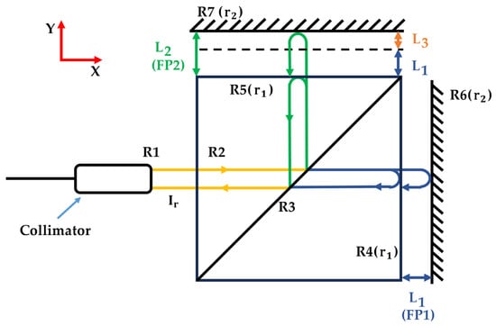
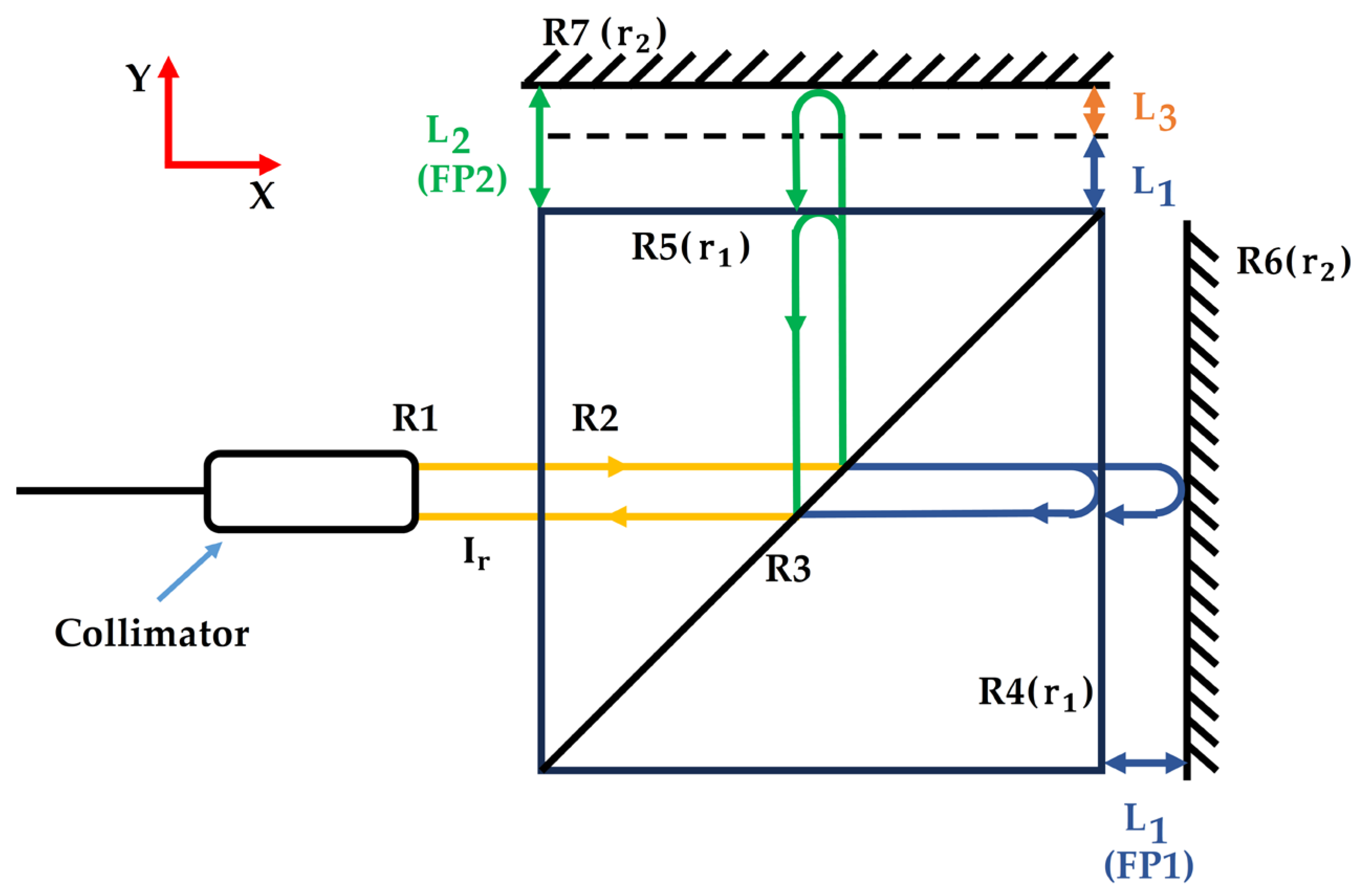
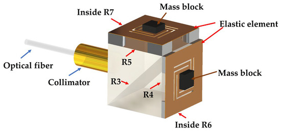
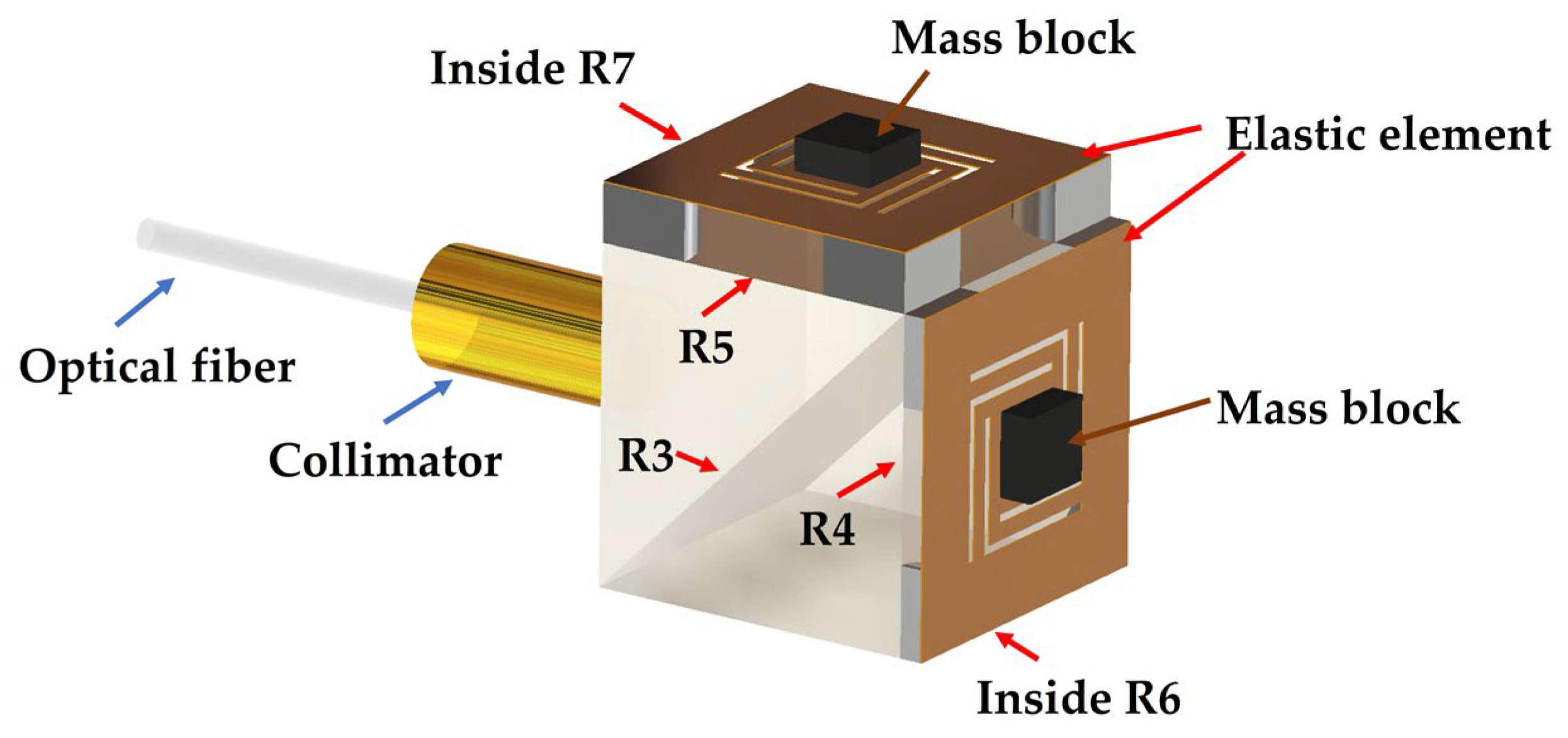
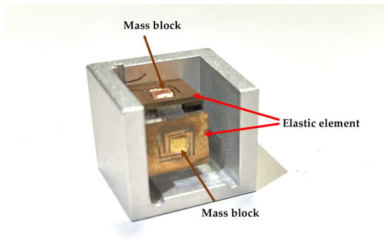
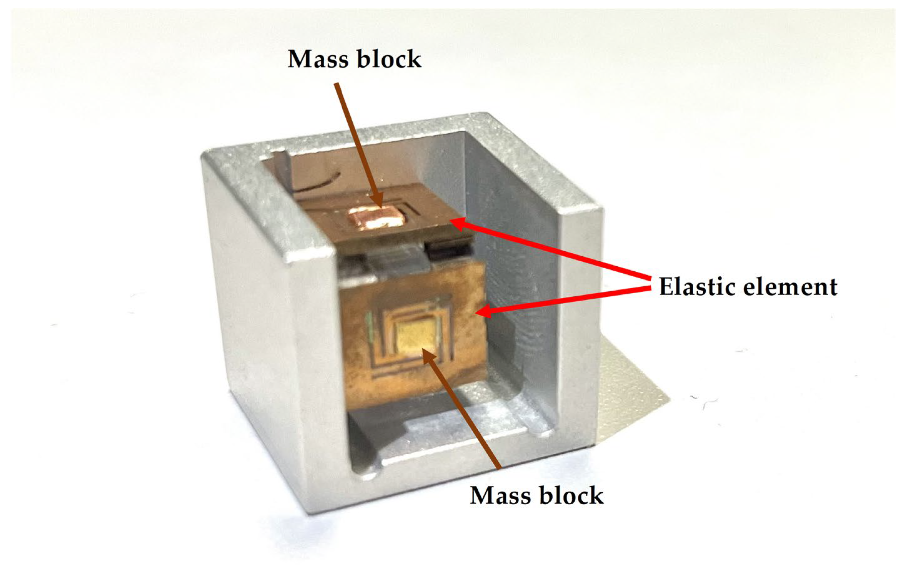
The core of an optical fiber FP sensor is the FP cavity, which typically consists of two parallel reflective surfaces. Figure 1 illustrates the optical principle of our optical fiber FP accelerometer: the optical reflective surfaces (R6 and R7) on the elastic element are parallel to the prism surfaces, forming extrinsic FP cavities. Specifically, two FP cavities are constructed within the sensor, located between R4 and R6 (FP1) and between R5 and R7 (FP2), respectively. The incident light enters these two cavities and undergoes multiple reflections and transmissions, generating the FP interference phenomenon. Subsequently, the optical signal returns along the original optical path to the collimator R1 via the beam-splitting surface R3. By analyzing the FP interference signals in these two sensing directions, the acceleration in the corresponding directions can be obtained. Figure 2 elucidates the internal structure of the sensor, in which the reflective surfaces R6 and R7 are positioned on the inner sides of two elastic elements. Each elastic element is integrated with a mass block. When acceleration is applied, the displacement induced by the mass blocks directly modulates the cavity lengths of FP1 and FP2. Figure 3 presents the photograph of the fabricated sensor prototype.

Figure 1. Sensor optical path structure analysis.

Figure 2. Internal structure diagram of the sensor.

Figure 3. Physical structure of the sensor.

According to the FP interference principle [9], the optical signal of the fiber FP sensor can be expressed as follows:

$$\begin{array}{c}I\left(\mathsf{\lambda }\right)={\displaystyle \frac{{\mathrm{r}}_1+{\mathrm{r}}_2-2\sqrt{{\mathrm{r}}_1{\mathrm{r}}_2}\cos \frac{4\pi \mathrm{n}\mathrm{L}}{\mathsf{\lambda }}}{1+{\mathrm{r}}_1{\mathrm{r}}_2-2\sqrt{{\mathrm{r}}_1{\mathrm{r}}_2}\cos \frac{4\pi \mathrm{n}\mathrm{L}}{\mathsf{\lambda }}}}{\mathrm{I}}_0\end{array}$$

(1)

where ${\mathrm{r}}_1,{\mathrm{r}}_2$ denote the reflectivities of the two cavity surfaces, $\mathrm{L}$ is the cavity length, $\mathsf{\lambda }$ is the optical wavelength, and $\mathrm{n}$ is the refractive index of the medium within the cavity; ${\mathrm{I}}_0$ represents light intensity.

For the low-finesse air-gap FP cavity employed in this sensor, as shown in Figure 1, the FP interference signal can be simplified using the double beam approximation in the wavelength domain as follows [10]:

$$\begin{array}{c}\left\{\begin{array}{c}\mathrm{I}{\left(\mathsf{\lambda }\right)}_{\mathrm{F}\mathrm{P}1}=({\displaystyle \frac{{\mathrm{I}}_1}{2}}+{\mathrm{I}}_2)+2\sqrt{{\displaystyle \frac{{\mathrm{I}}_1}{2}}{\mathrm{I}}_2}\cos \left({\displaystyle \frac{4\pi \mathrm{n}{\mathrm{L}}_1}{\mathsf{\lambda }}}+\pi \right)\\ {\mathrm{I}\left(\mathsf{\lambda }\right)}_{\mathrm{F}\mathrm{P}2}=({\displaystyle \frac{{\mathrm{I}}_1}{2}}+{\mathrm{I}}_3)+2\sqrt{{\displaystyle \frac{{\mathrm{I}}_1}{2}}{\mathrm{I}}_3}\cos \left({\displaystyle \frac{4\pi \mathrm{n}{\mathrm{L}}_2}{\mathsf{\lambda }}}+\pi \right)\end{array}\right.\end{array}$$

(2)

where ${\mathrm{I}}_1$ is the sum of the reflected light intensities from R4 and R5 (${\displaystyle \frac{{\mathrm{I}}_1}{2}}$: the splitting ratio of the splitting surface R3 is 50%:50%), ${\mathrm{I}}_2$ is the reflected light intensity from R6, and ${\mathrm{I}}_3$ is the reflected light intensity from R7. These light intensities are only related to the wavelength $\mathsf{\lambda }$ of the incident light and can thus be regarded as constants. Based on Equation (2), the interference characteristics of the internal cavities FP1 and FP2 can be described, respectively.

However, in addition to the FP interference, the unique optical configuration of the sensor introduces a second type of interference phenomenon. As shown in Figure 1, the two light beams reflected (${\mathrm{I}}_2, {\mathrm{I}}_3$) from surfaces R6 and R7 recombine at R3, generating Michelson interference. According to the optical path analysis, the arm length difference in this Michelson interference directly corresponds to the cavity length difference between FP1 and FP2, as expressed in Equation (3).

$$\begin{array}{c}{\mathrm{L}}_3=\left|{\mathrm{L}}_2-{\mathrm{L}}_1\right|\end{array}$$

(3)

In summary, the optical signal received by the sensor is a composite interference signal jointly generated by the FP1 cavity, the FP2 cavity, and the Michelson interference system formed by R6 and R7. By linearly superimposing the incoherent background intensities (DC) and the coherent interference modulation terms (AC) from the respective optical paths [11], the total spectral intensity returning to the collimator is derived as Equation (4):

$$\begin{array}{c}{\mathrm{I}}_{\mathrm{r}}\left(\mathsf{\lambda }\right)={\mathrm{I}}_1+{\mathrm{I}}_2+{\mathrm{I}}_3+2\mathsf{\eta }\sqrt{{\mathrm{I}}_1{\mathrm{I}}_2}\cos \left({\mathsf{\varphi }}_1+\pi \right)+2\mathsf{\eta }\sqrt{{\mathrm{I}}_1{\mathrm{I}}_3}\cos \left({\mathsf{\varphi }}_2+\pi \right)+2\sqrt{{\mathrm{I}}_2{\mathrm{I}}_3}\cos \left({\mathsf{\varphi }}_3\right)\end{array}$$

(4)

$$\begin{array}{c}{\mathsf{\varphi }}_1={\displaystyle \frac{4\pi \mathrm{n}{\mathrm{L}}_1}{\mathsf{\lambda }}}, {\mathsf{\varphi }}_2={\displaystyle \frac{4\pi \mathrm{n}{\mathrm{L}}_2}{\mathsf{\lambda }}}, {\mathsf{\varphi }}_3={\displaystyle \frac{4\pi \mathrm{n}{(\mathrm{L}}_2-{\mathrm{L}}_1)}{\mathsf{\lambda }}}\end{array}$$

(5)

where $\mathsf{\eta }={\displaystyle \frac{1}{\sqrt{2}}}$ accounts for the splitting ratio of the beam splitter R3 (50%:50%). It can be known from Equation (4) that the reflection spectrum of the sensor is mainly the linear superposition of three sets of cosine functions. Among them, the interference spectra of FP1 and FP2 correspond to the fourth and fifth terms of Equation (4), and ${\mathsf{\varphi }}_1,{\mathsf{\varphi }}_2$ correspond to the phases of FP1 and FP2. The Michelson interference spectrum corresponds to the sixth term of Equation (4). Through phase analysis, it is possible not only to determine the cavity lengths ${\mathrm{L}}_1$ and ${\mathrm{L}}_2$ of FP1 and FP2 but also to utilize the information carried by the Michelson interference to supplement and correct the measurement results.

When the sensor remains stationary, the cavity lengths of FP1 and FP2 are ${\mathrm{L}}_1,{\mathrm{L}}_2$, respectively. When subjected to acceleration excitation on the biaxial plane, the length of the FP cavity changes accordingly, defined as $∆{\mathrm{L}}_1\left(\mathrm{t}\right), ∆{\mathrm{L}}_2\left(\mathrm{t}\right)$. According to existing research [3], there exists the following linear relationship between acceleration and the variation in the cavity length of the optical fiber FP cavity:

$$\begin{array}{c}∆{\mathrm{L}}_1\left(\mathrm{t}\right)={\mathrm{K}}_1{\mathrm{a}}_1\left(\mathrm{t}\right), ∆{\mathrm{L}}_2\left(\mathrm{t}\right)={\mathrm{K}}_2{\mathrm{a}}_2\left(\mathrm{t}\right)\end{array}$$

(6)

where ${\mathrm{K}}_1, {\mathrm{K}}_2$ are the sensitivities of the sensor corresponding to the FP1 and FP2 directions, and ${\mathrm{a}}_1\left(\mathrm{t}\right),{\mathrm{a}}_2\left(\mathrm{t}\right)$ correspond to the accelerations in the X and Y directions, respectively.

2.2. Adaptive Filtering-Multiple Peaks Demodulation

Building upon the aforementioned analysis, decoupling the superimposed spectral signals is imperative for the single-optical-path multiplexed architecture involving multiple FP cavities. The aliased interference signals exhibit three distinct characteristic peaks in the spatial frequency domain. However, the time-varying nature of vibration signals induces dynamic evolution of the spatial peak frequency (${\mathrm{f}}_{\mathrm{p}\mathrm{e}\mathrm{a}\mathrm{k}}$) associated with each interference channel, rendering conventional static bandpass filters ineffective for precise signal separation. To circumvent this limitation, a dynamic filtering algorithm is implemented to decouple the superimposed interference spectra [12,13]. The spatial frequency peaks (${\mathrm{f}}_{\mathrm{p}\mathrm{e}\mathrm{a}\mathrm{k}}$) are accurately localized via spectral analysis enhanced by quadratic interpolation [14]. The dynamic bandwidth (${\mathrm{b}}_{\mathrm{w}}$) of the Gaussian filter bank is adaptively determined by the instantaneous peak frequency according to Equation (7), where ${\mathrm{f}}_{\mathrm{s}}$ denotes the equivalent sampling rate in the wavenumber domain and ${\mathrm{L}}_{\mathrm{s}\mathrm{i}\mathrm{g}}$ represents the spectral record length. This adaptive bandwidth ensures the integrity of the interference signal’s main lobe, thereby eliminating phase distortions typically induced by spectral truncation. The selection of the coefficients 3 and 0.1 is made to achieve noise suppression while ensuring signal integrity. Specifically, the value of 0.1 provides 10% relative bandwidth redundancy, which is used to compensate for frequency drift caused by environmental jitter and high-speed movement ($\pm 5\%$), thereby preventing signal truncation. Experimental verification has shown that the basic coefficient of 3 is the optimal value: if this value is less than 3, the “amplitude collapse” phenomenon will occur; if it exceeds 5, a large amount of out-of-band noise and oscillations will be introduced.

$$\begin{array}{c}{\mathrm{b}}_{\mathrm{w}}=\mathrm{m}\mathrm{a}\mathrm{x}\left(3\ast {\displaystyle \frac{{\mathrm{f}}_{\mathrm{s}}}{{\mathrm{L}}_{\mathrm{s}\mathrm{i}\mathrm{g}}}},0.1\ast {\mathrm{f}}_{\mathrm{p}\mathrm{e}\mathrm{a}\mathrm{k}}\right)\end{array}$$

(7)

After obtaining the adaptive dynamic bandwidth, the adaptive dynamic Gaussian filter bank is generated according to Equation (8). ${\mathrm{H}}_{\mathrm{n}}\left(\mathrm{f}\right)$ is a real-valued symmetric function with a zero-phase term. In the frequency domain, multiplying the complex spectrum of the original signal by ${\mathrm{H}}_{\mathrm{n}}\left(\mathrm{f}\right)$ only modifies the amplitude weighting of different frequency components, while preserving the original phase information.

$$\begin{array}{c}{\mathrm{H}}_{\mathrm{n}}\left(\mathrm{f}\right)={\mathrm{e}}^{-{\displaystyle \frac{{\left(\mathrm{f}-{\mathrm{f}}_{\mathrm{c}}\right)}^2}{2{\left(\frac{{\mathrm{b}}_{\mathrm{w}}}{2.355}\right)}^2}}}\end{array}$$

(8)

Then, a bilateral filter bank is constructed to filter and separate the aliasing optical signal in the frequency domain. The extracted frequency-domain complex signal is converted back to the wavelength domain via the inverse fast Fourier transform (IFFT) [15]. By leveraging the linear property of the IFFT and applying window functions for edge smoothing, the symmetry of the interference fringes is preserved. This ensures that the decoupled interference spectrum remains distortion-free, laying a solid foundation for the subsequent accurate phase extraction using the multi-peak least squares (MP-LS) method.

By combining Equation (5) to conduct phase analysis [16] on the separated FP interference signals, it can be known when ${\displaystyle \frac{4\pi \mathrm{n}\mathrm{L}}{\mathsf{\lambda }}}=\left(2\mathrm{m}+1\right)\pi$, the output light intensity of the interference signal is located at the peak position. When ${\displaystyle \frac{4\pi \mathrm{n}\mathrm{L}}{\mathsf{\lambda }}}=2\mathrm{m}\pi$, the output light intensity of the interference signal is in the trough position. When the light intensity of the $\mathrm{m}$ and $(\mathrm{m}+\mathrm{k})$ levels in the interference fringes is set to be located at the peak or trough, the corresponding wavelengths are ${\mathsf{\lambda }}_{\mathrm{m}}$ and ${\mathsf{\lambda }}_{\mathrm{m}+\mathrm{k}}$, respectively, where $\mathrm{m}$ is taken as an integer and the cavity length value $\mathrm{L}$ can be obtained, such as in Equation (9).

$$\begin{array}{c}\mathrm{L}={\displaystyle \frac{{\mathrm{k}\mathsf{\lambda }}_{\mathrm{m}}{\mathsf{\lambda }}_{\mathrm{m}+\mathrm{k}}}{2\mathrm{n}\left({\mathsf{\lambda }}_{\mathrm{m}+\mathrm{k}}-{\mathsf{\lambda }}_{\mathrm{m}}\right)}}\end{array}$$

(9)

According to the analysis of the multi-peak method principle [17], Equation (10) holds true:

$$\begin{array}{c}2\mathrm{n}\mathrm{L}\ast \mathrm{N}=2\mathrm{m}\pi \end{array}$$

(10)

$\mathrm{N}={\displaystyle \frac{2\pi }{{\mathsf{\lambda }}_{\mathrm{m}}}}$, where $\mathrm{N}$ denotes the wavenumber (the dependent variable in the linear regression equation). The interference peak order $\mathrm{m}$ (the independent variable in the linear regression equation) is an integer corresponding to the optical path difference of two coherent light beams being an integer multiple of the wavelength, indicating the order of the interference bright peak, and $\mathrm{d}$ is a constant. Simplifying the above linear regression equation yields Equation (11).

$$\begin{array}{c}\mathrm{N}={\displaystyle \frac{\pi \left(\mathrm{m}+\mathrm{d}\right)}{\mathrm{L}}}\end{array}$$

(11)

After obtaining the wavenumber $\mathrm{N}$, the least squares slope is obtained by fitting it by the least squares method [18], as shown in Equation (12).

$$\begin{array}{c}\mathrm{b}={\displaystyle \frac{\sum \left({\mathrm{m}}_{\mathrm{i}}-\overline{\mathrm{m}}\right)\left({\mathrm{N}}_{\mathrm{i}}-\overline{\mathrm{N}}\right)}{\sum {\left({\mathrm{N}}_{\mathrm{i}}-\overline{\mathrm{N}}\right)}^2}}\end{array}$$

(12)

Once the slope $\mathrm{b}$ of the least squares solution is obtained, the phase of the fitting result is compensated and corrected, and the cavity length can be further calculated:

$$\begin{array}{c}\mathrm{L}={\displaystyle \frac{\pi }{\mathrm{b}}}\end{array}$$

(13)

2.3. Triple-Interferometric Information Complementary Correction

After obtaining the initial values for the two FP cavity lengths (${\mathrm{L}}_1,{\mathrm{L}}_2$) and the Michelson arm length difference (${\mathrm{L}}_3$) using the multiple peaks–least squares method, a complementary model based on triple-interferometric information was constructed according to Equation (14), where ${\mathsf{ϵ}}_1,{\mathsf{ϵ}}_2,{\mathsf{ϵ}}_3$ represent the respective measurement error terms.

$$\begin{array}{c}\left\{\begin{array}{c}{\widehat{\mathrm{L}}}_1={\mathrm{L}}_1+{\mathsf{ϵ}}_1\\ {\widehat{\mathrm{L}}}_2={\mathrm{L}}_2+{\mathsf{ϵ}}_2\\ {\displaystyle {\widehat{\mathrm{L}}}_3={\mathrm{L}}_3+{\mathsf{ϵ}}_3}\\ {\displaystyle {\mathrm{L}}_3=\left|{\mathrm{L}}_2-{\mathrm{L}}_1\right|}\end{array}\right.\end{array}$$

(14)

The residual function $\mathrm{J}\left({\widehat{\mathrm{L}}}_1,{\widehat{\mathrm{L}}}_2\right)$ under the constraint of the triple-interferometric redundancy constraint is constructed from Equation (14), as shown in Equation (15).

$$\begin{array}{c}J\left({\widehat{\mathrm{L}}}_1,{\widehat{\mathrm{L}}}_2\right)={{\displaystyle \sum }}_{\mathrm{i}=1}^3{\mathsf{\omega }}_{\mathrm{i}}{\left({\widehat{\mathrm{L}}}_{\mathrm{i}}-{\mathrm{L}}_{\mathrm{i}}\right)}^2\end{array}$$

(15)

The residual function [19] is used to describe the minimum error of the demodulation system under the constraints of Equation (14). To address the differentiation issue of the absolute value term ${\mathrm{L}}_3=\left|{\mathrm{L}}_2-{\mathrm{L}}_1\right|$, the sign function $\mathrm{s}\mathrm{i}\mathrm{g}\mathrm{n} ({\mathrm{L}}_1-{\mathrm{L}}_2)$ is introduced in the partial derivatives to represent the relative magnitudes of the two FP cavity lengths. The weighting coefficients ${\mathrm{w}}_{\mathrm{i}}$ for the three sets of interference signals are determined based on the Weighted Least Squares (WLS) principle [20]. According to the Gauss–Markov theorem, the minimum variance estimation is achieved when the weights are assigned inversely to the variances of the measurements (${\mathrm{w}}_{\mathrm{i}}\propto 1/{\mathsf{\sigma }}_{\mathrm{i}}^2$). In optical frequency-domain sensing, the variance ${\mathsf{\sigma }}_{\mathrm{i}}^2$ of phase or length measurements is inversely proportional to the SNR, which is characterized by the spectral peak intensity ${\mathrm{I}}_{\mathrm{i}}$. Consequently, we define the weights as ${\mathrm{w}}_{\mathrm{i}}={\mathrm{I}}_{\mathrm{i}}/{\sum }_{\mathrm{j}=1}^3{\mathrm{I}}_{\mathrm{j}}$. This approach ensures that high-SNR signals dominate the convergence of the residual function, thereby reducing the global estimation error. The partial derivatives of ${\widehat{\mathrm{L}}}_1,{\widehat{\mathrm{L}}}_2$ to the residual functions $\mathrm{J}\left({\widehat{\mathrm{L}}}_1,{\widehat{\mathrm{L}}}_2\right)$ were ${\displaystyle \frac{\partial \mathrm{J}}{\partial {\widehat{\mathrm{L}}}_1}},{\displaystyle \frac{\partial \mathrm{J}}{\partial {\widehat{\mathrm{L}}}_2}}$, respectively, as shown in Equation (16).

$$\begin{array}{c}\left\{\begin{array}{c}{\displaystyle \frac{\partial \mathrm{J}}{\partial {\widehat{\mathrm{L}}}_1}}=2{\mathsf{\omega }}_1\left({\widehat{\mathrm{L}}}_1-{\mathrm{L}}_1\right)-2{\mathsf{\omega }}_3\ast \mathrm{sign}({\mathrm{L}}_1-{\mathrm{L}}_2)\left({\widehat{\mathrm{L}}}_3-{\mathrm{L}}_3\right)\\ {\displaystyle \frac{\partial \mathrm{J}}{\partial {\widehat{\mathrm{L}}}_2}}=2{\mathsf{\omega }}_2\left({\widehat{\mathrm{L}}}_2-{\mathrm{L}}_2\right)-2{\mathsf{\omega }}_3\ast \mathrm{sign}({\mathrm{L}}_1-{\mathrm{L}}_2)\left({\widehat{\mathrm{L}}}_3-{\mathrm{L}}_3\right)\end{array}\right.\end{array}$$

(16)

The gradient descent method [21] is employed to perform optimization by iteratively updating the values of ${\widehat{\mathrm{L}}}_1^{\mathsf{\tau }},{\widehat{\mathrm{L}}}_2^{\mathsf{\tau }}$, with the update strategy specified in Equation (17).

$$\begin{array}{c}\left\{\begin{array}{c}{\mathrm{L}}_1^{\left(\mathsf{\tau }+1\right)}={\widehat{\mathrm{L}}}_1^{\mathsf{\tau }}-\alpha \ast {\displaystyle \frac{\partial \mathrm{J}}{\partial {\widehat{\mathrm{L}}}_1^{\mathsf{\tau }}}}\\ {\mathrm{L}}_2^{\left(\mathsf{\tau }+1\right)}={\widehat{\mathrm{L}}}_2^{\mathsf{\tau }}-\alpha \ast {\displaystyle \frac{\partial \mathrm{J}}{\partial {\widehat{\mathrm{L}}}_2^{\mathsf{\tau }}}}\end{array}\right.\end{array}$$

(17)

where $\mathsf{\tau }$ denotes the iteration index and $\alpha$ is the learning rate. The optimization process continues until the convergence criterion specified in Equation (18) is met.

$$\begin{array}{c}\left|{\mathrm{J}}^{\left(\mathsf{\tau }+1\right)}-{\mathrm{J}}^{\mathsf{\tau }}\right|<\epsilon \end{array}$$

(18)

where $\epsilon$ is the predefined threshold, and ${\mathrm{J}}^{\mathsf{\tau }}$ denotes the value of the objective function at the $\mathsf{\tau }$ iteration.

Based on the above analysis, a complementary correction model is proposed. Under the constraints of Equation (14), a residual function is constructed and the two global optimal solutions that make the residual function take the minimum value are found, that is, the final optimized cavity lengths ${\widehat{\mathrm{L}}}_1^{\mathsf{\tau }},{\widehat{\mathrm{L}}}_2^{\mathsf{\tau }}$. We introduce ${\mathrm{L}}_3$ increase constraints, and then obtain more accurate ${\widehat{\mathrm{L}}}_1^{\mathsf{\tau }},{\widehat{\mathrm{L}}}_2^{\mathsf{\tau }}$. At the same time, the stability of the demodulation system is enhanced.

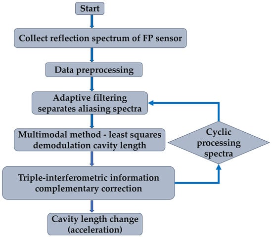
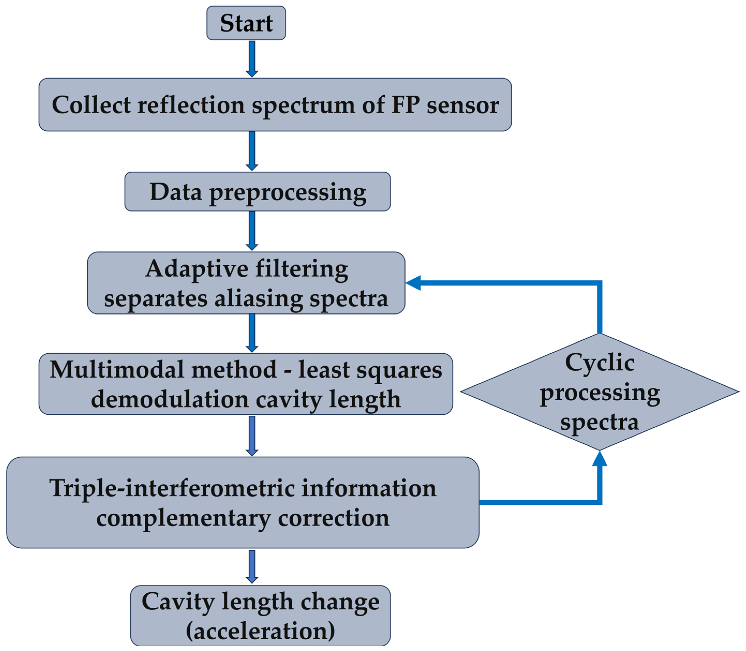
Based on the above analysis, this paper proposes an adaptive filtering–multiple peaks–cooperative least squares (AF-MP-LS) algorithm to process multi-dimensional acceleration signals and develops a triple-interferometric information complementary model to compensate and correct the target cavity lengths, thereby improving demodulation accuracy. The algorithm flow is shown in Figure 4: first, frequency analysis of the aliased optical signals is performed, and an adaptive Gaussian filter bank is generated according to peak frequency variations to separate the aliased signals; then, the multiple-peak least squares method is employed to demodulate the separated optical signals. Subsequently, a cavity length compensation correction model is constructed based on the complementary characteristics of triple-interferometric information to enhance the final demodulation accuracy of the target cavity lengths; finally, subsequent spectral data are processed iteratively. The variations in the target cavity lengths are derived, and multi-dimensional acceleration is thereby calculated.

Figure 4. Algorithm flow chart.

3. Simulation Analysis

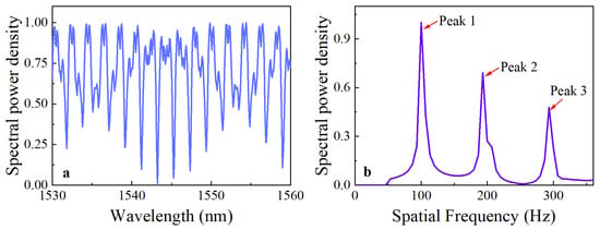
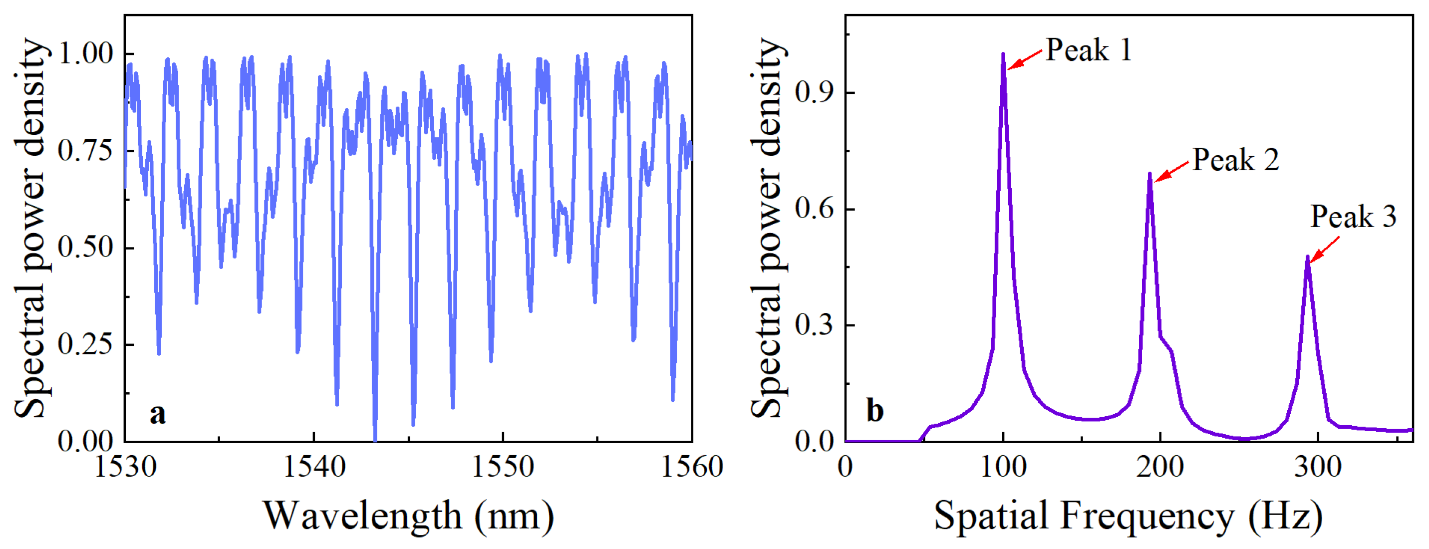
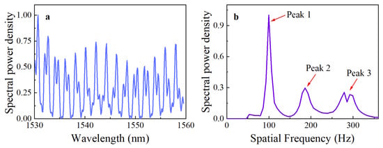
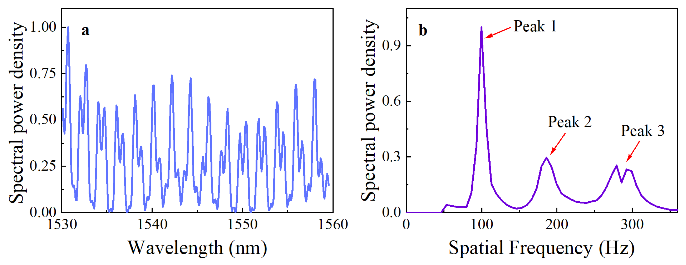
For the optical fiber FP two-dimensional acceleration sensor with the structure shown in Figure 1, the initial cavity lengths are set to 606.11 µm and 1748.90 µm, respectively. The cavity length variation follows a 100 Hz sinusoidal signal. Within the wavelength range of 1530–1560 nm, the reflection spectra of the sensor are simulated. Based on the optical path analysis, there are three groups of interference signals, and three sets of interference peaks are extracted via frequency-domain analysis. Figure 5 presents the frequency-domain transformation results of the normalized analog reflectance spectral signals.

Figure 5. Simulated aliasing signal. (a) Wavelength domain. (b) Frequency domain.

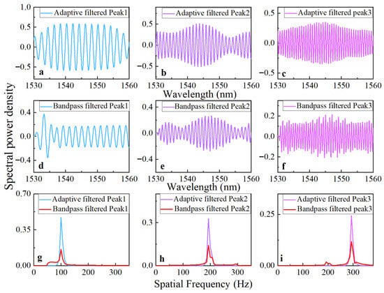
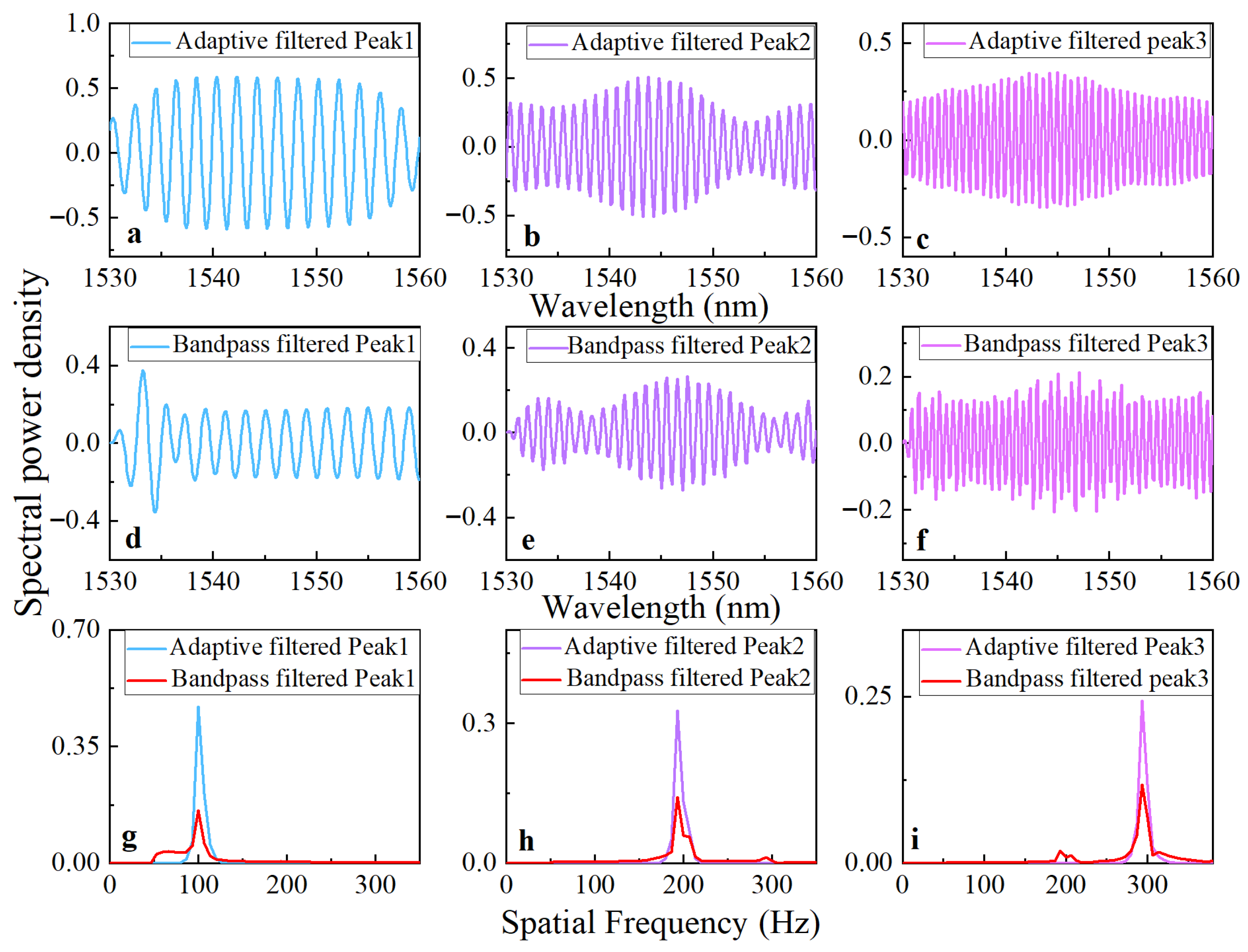
According to Figure 5b, there are three dominant frequency components in the aliased signal, denoted as Peak1 (carrying FP1 cavity length information), Peak2 (Michelson interferes with the arm length difference information), and Peak3 (carrying FP2 cavity length information). Based on the frequency characteristics of these three groups of signals, a corresponding dynamic Gaussian filter bank is generated to separate the aliased signals. The results of signal separation using the adaptive filter are compared with those using the bandpass filter, as shown in Figure 6.

Figure 6. Comparison of adaptive filtering and bandpass filtering separation. (a,d) Peak1 signal. (b,e) Peak2 signal. (c,f) Peak3 signal. (g) Peak1 signal frequency-domain comparison. (h) Peak2 signal frequency-domain comparison. (i) Peak3 signal frequency-domain comparison.

It is evident that the separation resolution of the adaptive filter is higher than that of the bandpass filter. The signals separated by the adaptive filter are closer to the target frequency band and exhibit a smoother separation effect, alleviating the abrupt transition of signals when passing through the filter.

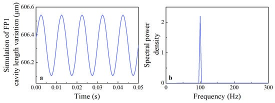
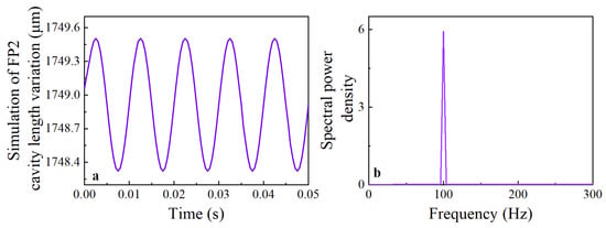
Initial length estimates are extracted from the separated three groups of optical signals using the MP-LS method, then further refined via a triple-interferometric correction model to yield the final optimized values. The cavity length values of FP1 (Peak1) and FP2 (Peak3) are compensated by using the information demodulated by Peak2. The algorithm’s performance in demodulating cavity length variations was simulated at a vibration frequency of 100 Hz. Spectral data within 0.05 s under 100 Hz vibration were processed to obtain the corresponding cavity length changes. The processing results are shown in Figure 7 and Figure 8.

Figure 7. Simulating FP1 signal. (a) FP1 cavity length change. (b) Frequency-domain signal.

Figure 8. Simulating FP2 signal. (a) FP2 cavity length change. (b) Frequency-domain signal.

The frequency in Figure 6 and Figure 7 is 100 Hz, which is consistent with the vibration frequency.

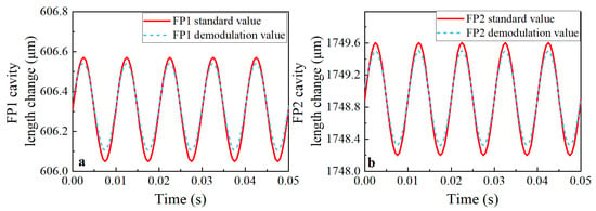
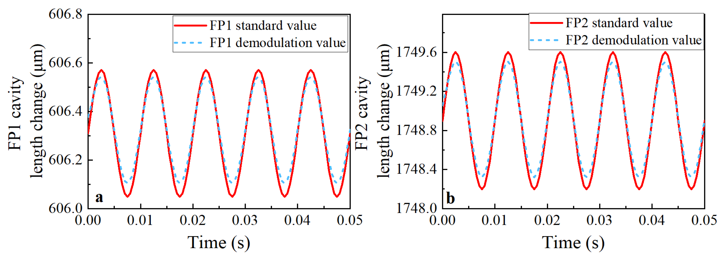
The initial measurement lengths of the two FP cavities of the fiber FP two-dimensional accelerometer (FP1: 606.11 µm, FP2: 1748.90 µm) were taken as references. A standard sinusoidal vibration signal with a vibration frequency of 100 Hz that conforms to the dynamic variation law of the cavity lengths of FP1 and FP2 was generated through simulation, serving as the verification standard for the demodulation effect of the algorithm. The simulated cavity length change is compared with the cavity length change after demodulation, as shown in Figure 9:

Figure 9. Simulation of the change in cavity length and the change in demodulated cavity length. (a) Change in cavity length of FP1. (b) Change in cavity length of FP2.

The average absolute error of the simulated cavity length change and the demodulated cavity length change is 0.00386 µm, and the correlation coefficient between the two is 0.9967. Therefore, the algorithm can effectively process multi-dimensional aliasing vibration signals, and dynamic filtering can separate aliasing signals more efficiently and has higher demodulation accuracy compared with traditional demodulation methods.

4. Experimental Validation

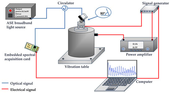
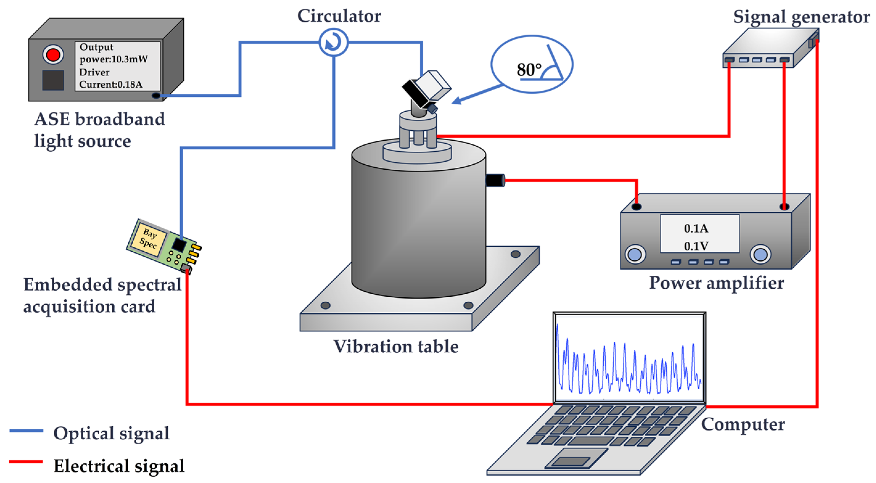
An experimental test system was constructed using the optical fiber FP two-dimensional acceleration sensor to experimentally verify the proposed demodulation algorithm. The system mainly includes a shaking table (Brüel & Kjær (B&K), Nærum, Denmark (Model 4808)), operating frequency range: 5–2000 Hz), an ASE broadband light source (Amonics Limited, Hong Kong, China (Model ASE-CL-10-8)), a spectral data acquisition card (BaySpec Inc., San Jose, CA, USA (embedded model); acquisition range: 1525–1565 nm; sampling frequency: 2000 Hz; wavelength resolution: 0.1 nm), an optical circulator, the two-dimensional FP accelerometer and a computer. The experimental system is illustrated in Figure 10. The sensor is fixed on the shaker at an $80°$ angle to the horizontal plane, and the shaker applies 100 Hz vertical vibration. Light emitted by the ASE broadband light source is transmitted to the sensor via the optical circulator; the reflected light carrying cavity length information is returned along the original path to the optical circulator and then received by the spectral acquisition card to obtain the reflected spectrum. The reflected spectral data is sent to the computer for processing, and signal processing is performed according to the proposed algorithm to derive the cavity length variation in the FP sensor. Based on the laboratory’s previous research [8], the sensor’s sensitivities under 100 Hz vibration are known: 3.93 µm/g for the X-axis (FP1) and 4.19 µm/g for the Y-axis (FP2). Although the shaker supports a wide frequency range, the experimental evaluation was primarily conducted at 100 Hz, which is within the linear working bandwidth of the sensor (its natural frequency is approximately 287 Hz). This ensures that the mechanical response is not affected by resonance distortion, allowing the algorithm itself to be evaluated. Since the spectral acquisition card operates at 2000 Hz, the system provides 20 sampling points per cycle at 100 Hz vibration, which strictly satisfies the Nyquist criterion.

Figure 10. Experimental test system.

When the angle between the sensor and the horizontal plane is $80°$, the vertical upward 100 Hz vibration is applied, and the acceleration excitation of the sensor’s double FP cavity is obtained by the acceleration (a) decomposition in the vertical direction (${\mathrm{a}}_{\mathrm{X}\left(\mathrm{FP}1\right)}=\mathrm{a}·\sin 80°, {\mathrm{a}}_{\mathrm{Y}\left(\mathrm{FP}2\right)}=\mathrm{a}·\cos 80°$). Figure 11a presents the normalized instantaneous mixed spectrum acquired by the data acquisition card, while Figure 11b shows the corresponding spatial frequency spectrum.

Figure 11. Mixed spectra. (a) Wavelength domain. (b) Frequency domain.

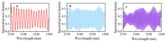
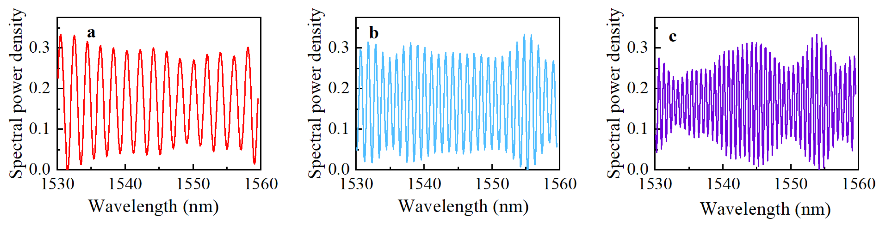
The spectral data acquisition card employed in this experiment is a Bay Spec embedded integrated spectrum analyzer, with 301 sampling points configured per single spectrum. Owing to the constraint on the number of sampling points, the peak frequency characteristics in the frequency domain are insufficiently distinct, thus enhancing the resolution via quadratic interpolation. Three groups of separated signals are obtainable via filtering the interpolated aliased signal, as shown in Figure 12.

Figure 12. Signal separation diagram. (a) Peak1 signal separation. (b) Peak2 signal separation. (c) Peak3 signal separation.

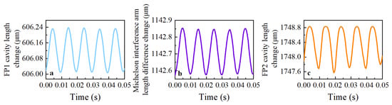
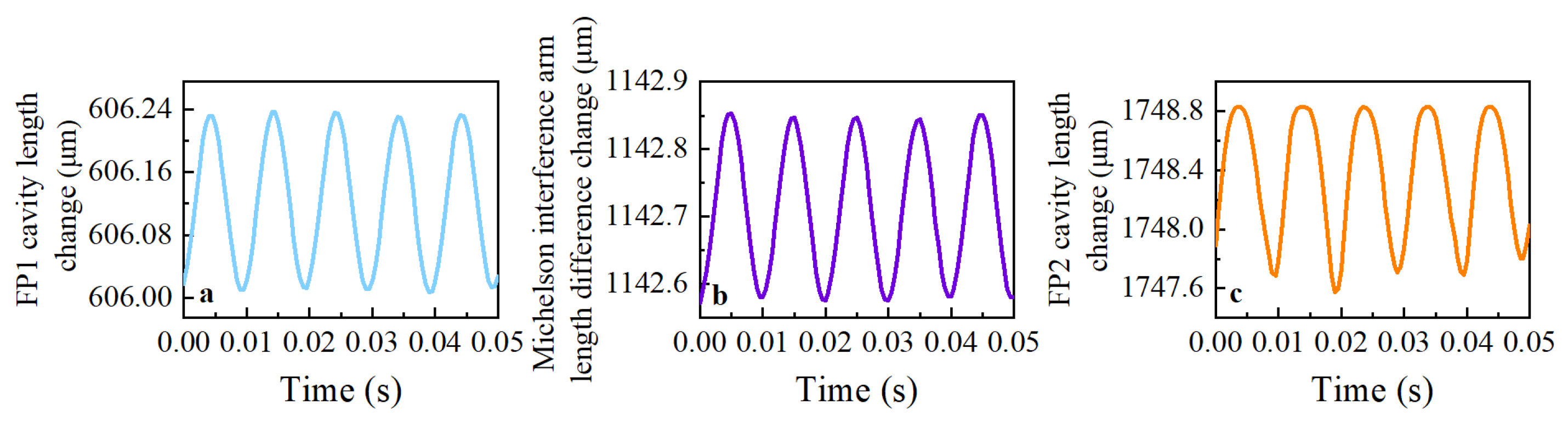
The three separated optical signals are demodulated via the multiple peaks–least squares method, and the cavity lengths corresponding to the first group of separated signals are derived as 606.02 µm, 1142.57 µm, and 1747.90 µm. The remaining spectral data are processed iteratively to obtain the corresponding three groups of variations in the original lengths. The results are presented in Figure 13.

Figure 13. Change in initial cavity length. (a) Change in cavity length of FP1 (Peak1). (b) Change in arm length difference of Michelson’s interference (Peak2). (c) Change in cavity length of FP2 (Peak3).

Based on the theoretical framework presented in Section 2.3, we established a self-compensation correction model for the triple-interferometric system. By retrieving information embedded in the three sets of peak signals to refine the target cavity length measurements, the demodulation accuracy is significantly improved.

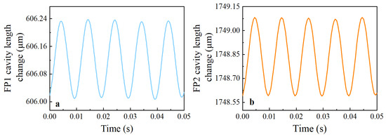
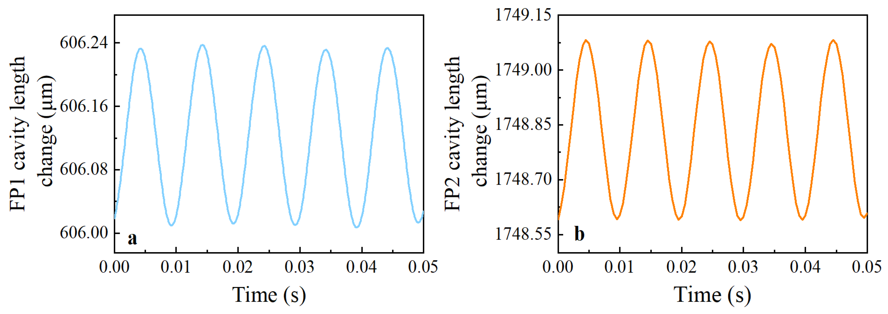
The information demodulated by the signal of Peak2 is used to compensate and correct the cavity length values demodulated by Peak1 and Peak3, so as to obtain more accurate cavity length values. The change in the cavity lengths of FP1 and FP2 after compensation correction is shown in Figure 14.

Figure 14. Change in cavity length after correction. (a) Change in cavity length of FP1. (b) Change in cavity length of FP2.

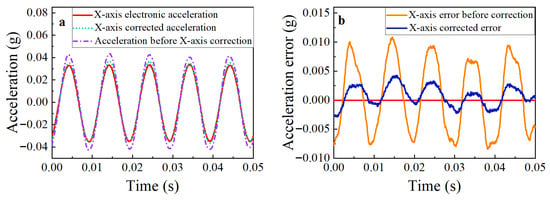
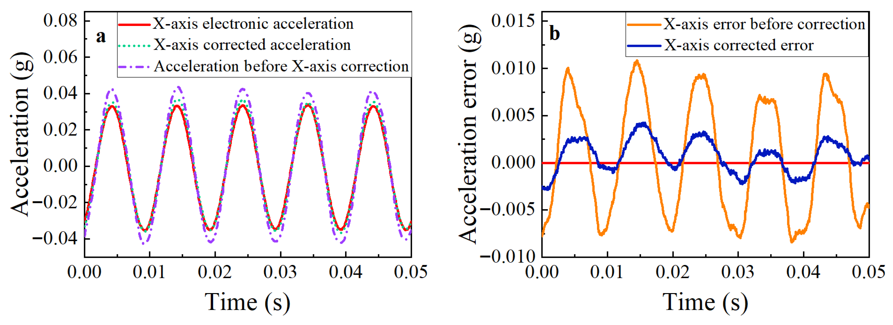
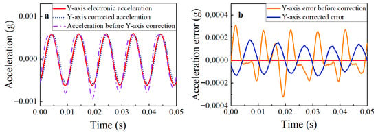
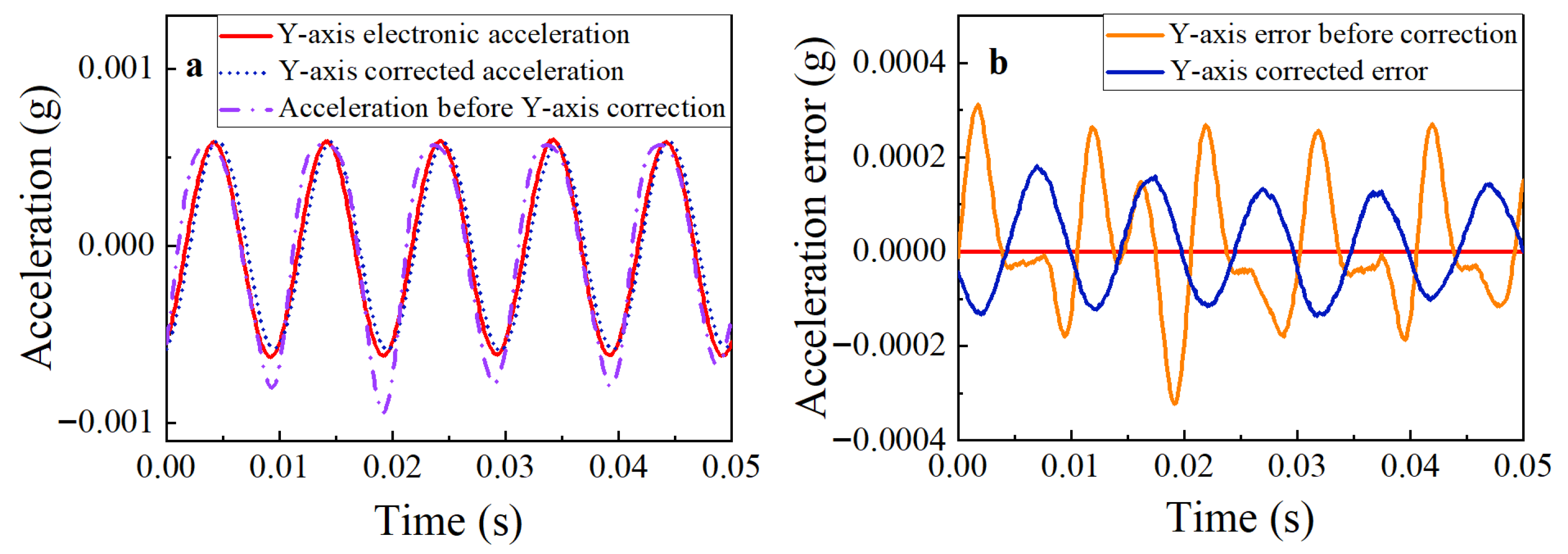
According to the electronic acceleration data and the uniaxial sensitivity of the sensor, the demodulated acceleration values are obtained by integrating the cavity length variations. The pre-correction and post-correction demodulation results of the FP1 (X-axis) and FP2 (Y-axis) cavities are compared with the corresponding electronic accelerometer readings. The demodulated acceleration values and their corresponding frequency-domain analysis results are presented in Figure 15 and Figure 16.

Figure 15. Acceleration of X-axis. (a) Three groups of X-axis accelerations. (b) X-axis accelerations error.

Figure 16. Acceleration of Y-axis. (a) Three groups of Y-axis accelerations. (b) Y-axis accelerations error.

As can be seen in Figure 14a and Figure 15a, the corrected X-axis and Y-axis accelerations are closer to the electronic accelerometer readings than their pre-correction counterparts. Meanwhile, Figure 14b and Figure 15b demonstrate that the overall errors of the corrected X-axis and Y-axis accelerations are smaller than the pre-correction acceleration errors.

To further evaluate the robustness and consistency of the calibration algorithm, we conducted additional vibration experiments at 45° and 60° under 100 Hz excitation. Table 1 summarizes the root mean square error (RMSE) of the biaxial system under different excitation conditions. It can be observed that the discrepancy in RMSE improvement rates at 80° (70.90% for the X-axis versus 30.60% for the Y-axis) is mainly attributed to the uneven projection of the acceleration vector. At 80°, the Y-axis (FP2) only bears a small fraction of the total acceleration, resulting in SNR being far lower than that of the X-axis. However, when the vibration angle was adjusted to 45° and 60°, the improvement rate of the Y-axis increased significantly to 57.20% and 51.69%, respectively. These results demonstrate that the proposed algorithm exhibits stable performance and can deliver consistent effectiveness with sufficient excitation intensity, regardless of the cavity length differences.

Table 1. RMSE comparison of accelerometer data before and after correction from different perspectives.

Angle	Axis (Sensor)	RMSE Before Correction (g)	RMSE After Correction (g)	Improvement
45°	X-axis (FP1)	0.0333	0.0105	68.47%
	Y-axis (FP2)	0.0535	0.0229	57.20%
60°	X-axis (FP1)	0.0451	0.0238	47.23%
	Y-axis (FP2)	0.0207	0.0100	51.69%
80°	X-axis (FP1)	0.0062	0.0018	70.90%
	Y-axis (FP2)	0.0137	0.0095	30.60%

To evaluate the performance of the proposed AF-MP-LS demodulation algorithm, it was compared with two methods developed in recent years: the Multiorder Cavity Length Estimation Algorithm (MCLE) [21] and the Cavity Length Sequence Matching Algorithm (CLSM) [22]. Measured data under 100 Hz–45° vibration conditions were utilized to demodulate X-axis and Y-axis acceleration signals, with the measurements from a high-precision electronic accelerometer serving as the standard reference. The demodulation accuracy was quantitatively assessed using the root mean square error (RMSE). As summarized in Table 2, the AF-MP-LS algorithm consistently maintains the minimum residuals relative to the reference signal, outperforming both MCLE and CLSM. Specifically, the RMSE of the proposed algorithm is 0.0115 g for the X-axis and 0.0148 g for the Y-axis. The superiority of AF-MP-LS primarily stems from its integration of adaptive filtering with a multi-interference information complementary mechanism. Due to phase–order matching deviations or limited dynamic tracking capabilities under complex vibrations, MCLE and CLSM exhibit pronounced oscillatory characteristics in their error curves. In contrast, the proposed AF-MP-LS effectively suppresses such fluctuations. By leveraging complementary information from multiple interference spectra, the algorithm ensures high demodulation accuracy and stability.

Table 2. Benchmarking of AF-MP-LS against MCLE and CLSM algorithms.

Demodulation Algorithm	X-Axis RMSE (g)	Y-Axis RMSE (g)
MCLE [22]	0.0397	0.0228
CLSM [23]	0.0215	0.0222
AF-MP-LS (Our work)	0.0115	0.0148

5. Conclusions

In view of the multi-channel interference spectral aliasing phenomenon in the multi-FP cavity multiplexing structure in the optical fiber FP multi-dimensional accelerometer, which leads to the problems of low aliasing signal separation efficiency and limited cavity length demodulation accuracy of the traditional cavity length demodulation algorithm, an adaptive filtering multiple peaks cooperative least squares algorithm (AF-MP-LS) is proposed and verified in this paper. The adaptive Gaussian filter is used to efficiently separate the aliasing interference signals, which improves the signal separation efficiency. The multiple peaks method combined with the least squares method is used to demodulate the cavity length, which improves the resolution of demodulation and overcomes the problem of limited spectral dynamic range during cavity length demodulation. At the same time, using the multi-peak information carried by the multi-FP cavity multiplexing structure, a complementary correction mechanism for triple-interferometric information is proposed, which suppresses the crosstalk noise and improves the demodulation accuracy of the target cavity length. Through experimental verification, the mean square error of the acceleration value obtained after correction decreased by 0.0044 g compared with that before correction and relatively decreased by 70.9%.

References

- Davydov, V.S. Recognition of Incipient Defects in the Units of Ship Machinery by Vibrodiagnostics Based on Optimum Decision Rules. Russ. J. Nondestr. Test. 2019, 55, 185–191. [Google Scholar] [CrossRef] [Scilit]
- Laudati, A.; Mennella, F.; Giordano, M.; D’Altrui, G.; Tassini, C.C.; Cusano, A. A fiber-optic Bragg grating seismic sensor. IEEE Photonics Technol. Lett. 2007, 19, 1991–1993. [Google Scholar] [CrossRef] [Scilit]
- Ran, Z.L.; Lu, E.; Rao, Y.J.; Ni, M.; Peng, F.; Zeng, D.H. Fiber-optic Fabry-Perot interferometer tip accelerometer fabricated by laser-micromachining. In Proceedings of the 21st International Conference on Optical Fiber Sensors, Ottawa, ON, Canada, 15–19 May 2011. [Google Scholar] [CrossRef] [Scilit]
- Ogawal, Y.; Takagi, K. An assessment of the effect of hull girder vibration on the statistical characteristics of wave loads. Int. J. Nav. Archit. Ocean Eng. 2011, 3, 80–85. [Google Scholar] [CrossRef] [Scilit]
- Yu, H.Y.; Zhao, L.; Zhang, K.; Wu, Y.H. Study on wind load performance for L Type Aerial Work Suspended Platform. In Proceedings of the 3rd International Conference on Manufacturing Science and Engineering (ICMSE 2012), Xiamen, China, 27–29 March 2012. [Google Scholar] [CrossRef] [Scilit]
- Ma, G.F.; Chen, T.G. Wind-induced Vibration Analysis of Wind Fence Structure. In Proceedings of the International Conference on Vibration, Structural Engineering and Measurement (ICVSEM 2012), Shanghai, China, 19–21 October 2012. [Google Scholar] [CrossRef] [Scilit]
- Lei, Y.J.; Zhang, L.S.; Pan, Q.S.; Hu, P.H.; Huang, Q.X.; Li, R.J. Two-Dimensional Low-Frequency Optical Accelerometer with High Accuracy and Low Cross-Axis Sensitivity. IEEE Trans. Instrum. Meas. 2023, 72, 1–9. [Google Scholar] [CrossRef] [Scilit]
- Zheng, B.; Liu, H.; Pan, Z.; Chen, X.; Wang, L.; Fan, D. A High-Sensitivity Dual-Axis Accelerometer with Two FP Cavities Assembled on Single Optical Fiber. Sensors 2022, 22, 9614. [Google Scholar] [CrossRef] [Scilit] [PubMed]
- Li, Z.Y.; Wang, S.; Jiang, J.F.; Sang, M.; Yu, Y.; Liu, W.Y.; Zhang, P.; Liu, T.G. Real-Time Pressure Measurement Method Based on Rapid Phase Demodulation of Multi-Cavities F-P Sensor. IEEE Sens. J. 2021, 21, 26624–26630. [Google Scholar] [CrossRef] [Scilit]
- Kang, J.; Chen, H.; Zhang, X.; Zhang, J.; Guo, Z.; Wang, W. Valley-positioning-assisted discrete cross-correlation algorithm for fast cavity length interrogation of fiber-optic Fabry–Perot sensors. Measurement 2022, 198, 111411. [Google Scholar] [CrossRef] [Scilit]
- Wang, Y.; Yan, Y.; Yuan, W.; Lian, Z.; Chen, D.; Tao Lau, A.P.; Yu, C.; Lu, C. Highly sensitive gas pressure sensor based on the hollow core Bragg fiber and harmonic Vernier effect. Opt. Lett. 2023, 48, 1990–1993. [Google Scholar] [CrossRef] [Scilit] [PubMed]
- Fukushima, N.; Tsubokawa, T.; Maeda, Y. Vector Addressing for Non-Sequential Sampling in Fir Image Filtering. In Proceedings of the 26th IEEE International Conference on Image Processing (ICIP), Taipei, Taiwan, 22–25 September 2019. [Google Scholar]
- He, J.J.; Song, C.; Luo, Q.W.; Yang, C.H.; Gui, W.H. EWT-ASG: Empirical Wavelet Transform With Adaptive Savitzky-Golay Filtering for TDLAS. IEEE Photonics J. 2020, 12, 1–12. [Google Scholar] [CrossRef] [Scilit]
- Chen, X.; Xiang, Y.; Feng, Y.T. Selection of interpolation methods used to mitigate spectral misregistration of imaging spectrometers. Guangpuxue Yu Guangpu Fenxi 2011, 31, 1147–1150. [Google Scholar] [CrossRef]
- Jang, I.G.; Jo, G.D. Study on the latency efficient IFFT design method for low latency communication systems. In Proceedings of the International Symposium on Intelligent Signal Processing and Communication Systems (ISPACS), Phuket, Thailand, 24–27 October 2016. [Google Scholar]
- Li, Y.; Wang, Y.; Xiao, L.; Bai, Q.; Liu, X.; Gao, Y.; Zhang, H.; Jin, B. Phase Demodulation Methods for Optical Fiber Vibration Sensing System: A Review. IEEE Sens. J. 2022, 22, 1842–1866. [Google Scholar] [CrossRef] [Scilit]
- Li, C.X.; Zhao, X.Y.; Qi, H.C.; Wang, Z.Z.; Xu, Y.F.; Han, X.; Huang, J.; Gao, M.; Chen, K. Integrated fiber-optic Fabry-Perot vibration/acoustic sensing system based on high-speed phase demodulation. Opt. Laser Technol. 2024, 169, 110131. [Google Scholar] [CrossRef] [Scilit]
- Su, P.; Xu, L.Y.; Yang, J. 1D regularization inversion combining particle swarm optimization and least squares method. Appl. Geophys. 2023, 20, 77–87. [Google Scholar] [CrossRef] [Scilit]
- Ling, C.; Qi, L.Q.; Zhou, G.L.; Caccetta, L. The SC1 property of an expected residual function arising from stochastic complementarity problems. Oper. Res. Lett. 2008, 36, 456–460. [Google Scholar] [CrossRef] [Scilit]
- Kay, S.M. Fundamentals of Statistical Signal Processing: Estimation Theory; Prentice Hall: Hoboken, NJ, USA, 1995; Volume 37, pp. 465–466. [Google Scholar]
- Hanna, A.I.; Mandic, D.P. A data-reusing nonlinear gradient descent algorithm for a class of complex-valued neural adaptive filters. Neural Process. Lett. 2003, 17, 85–91. [Google Scholar] [CrossRef] [Scilit]
- Shen, Y.; Jiang, Y.; Xie, S.; Hu, C. Multiorder Cavity Length Estimation Algorithm of Low-Fineness Sapphire Fabry–Perot Interferometers for Strain Measurement Under Ultrahigh Temperature. IEEE Sens. J. 2025, 25, 16873–16880. [Google Scholar] [CrossRef] [Scilit]
- Nie, L.; Li, X.; Chen, H.; Zhang, J.; Chen, H.; Zhao, X.; Wang, S.; Liu, G. Cavity Length Sequence Matching Algorithm Based on Combined Valley Peak Positioning for Fiber-Optic Fabry-Perot Sensors. Photonics 2022, 9, 451. [Google Scholar] [CrossRef] [Scilit]
Disclaimer/Publisher’s Note: The statements, opinions and data contained in all publications are solely those of the individual author(s) and contributor(s) and not of MDPI and/or the editor(s). MDPI and/or the editor(s) disclaim responsibility for any injury to people or property resulting from any ideas, methods, instructions or products referred to in the content. |
© 2026 by the authors. Licensee MDPI, Basel, Switzerland. This article is an open access article distributed under the terms and conditions of the Creative Commons Attribution (CC BY) license.