


Abstract
A primary bottleneck in deploying Fiber Bragg Grating (FBG) sensors lies in their inherent dual sensitivity to thermal and mechanical variations, which mandates robust decoupling mechanisms for precise parameter extraction. To address this persistent cross-sensitivity issue, this study introduces a novel interrogation scheme that integrates a Convolutional Neural Network with a Bidirectional Long Short-Term Memory (CNN-BiLSTM) architecture. Instead of relying on conventional peak-tracking algorithms or isolated central wavelengths, our proposed data-driven strategy directly mines structural features from the full reflection spectra, thereby substantially mitigating cross-interference errors. The experimental results reveal that the coefficients of determination (R2) for strain and temperature prediction reach 99.37% and 99.75% each, while the root mean square errors (RMSEs) are 13.51 µε and 1.42 °C, respectively. The proposed method requires only a single FBG sensor, which reduces the sensor requirements, showing great potential in sensing applications requiring low costs and high adaptability. In addition, in some special environments, temperature information cannot be obtained, so we utilize another reference FBG to realize the temperature compensation. Meanwhile, we proposed a spectral differencing method (SDM) by differencing the spectra of the two FBGs to obtain the spectra containing only strain information and sent them as a dataset for model training, with a 4-times improvement in accuracy over traditional compensation methods. Finally, we also explored the application of the system for distributed FBGs, achieving an absolute peak wavelength interrogation precision of approximately ±0.02 nm. The system is expected to be applied in the field of structural health monitoring, which is promising even in harsh environments.
1. Introduction
Driven by the rapid iterations in optical communication networks, fiber-optic sensing has evolved into a robust diagnostic paradigm. Unlike conventional electrical measurement tools, optical devices exhibit inherent immunity to electromagnetic perturbations, alongside highly compact form factors and exceptional anti-corrosive properties, making them indispensable for complex multi-parameter monitoring in challenging environments [1,2]. Among all kinds of optical fiber sensors, FBG sensors are widely used due to their characteristic of wavelength absolute encoding. They are widely used in many industrial areas, such as pipelines, civil engineering, aerospace and other fields. Accurately decoding sensor signals, especially tracking the slight changes in Bragg wavelength caused by external, measured parameters, remains a core technical challenge for fiber Bragg grating (FBG) demodulation systems [3,4]. Real-world deployments frequently expose these sensors to fluctuating thermal conditions, which introduces parasitic wavelength shifts and consequently compromises strain measurement fidelity [5]. Although several specialized sensor structures have been reported to address this shortcoming [6,7,8,9,10], they typically impose strict fabrication requirements. Moreover, these approaches remain heavily constrained by the traditional Sensitivity Matrix Method (SMM), which inevitably introduces significant errors when nonlinear sensitivity variations occur during the actual measurement process. For multi-parameter sensors, especially sensors with cross-sensitivity among multiple parameters, it is difficult to demodulate them accurately just by a calibration sensitivity matrix with fixed matrix elements. It can be predicted that once the testing surrounding is changed, results obtained from the sensitivity matrix method may show large errors. Therefore, it is still urgent to further research and develop a high-accuracy and low-complexity interrogation system.
In recent years, machine learning (ML) paradigms have gained substantial traction across various analytical domains [11]. Within the field of optical fiber sensing, ML techniques have demonstrated remarkable potential. For instance, Djurhuus et al. [12] leveraged ML to precisely identify Bragg peak positions for thermal measurements, while Sarkar et al. [13] explored its viability for temperature-independent strain interrogation. Similarly, Kikuchi et al. [14] validated the efficacy of ML in enhancing the simultaneous measurement accuracy of tilted FBG (TFBG) sensors. Particularly for multi-parameter sensing scenarios plagued by nonlinear crosstalk, data-driven approaches offer a robust alternative to conventional demodulation strategies. As a sophisticated subset of ML, deep learning has increasingly been adopted to tackle complex fiber-optic signal processing. Convolutional neural networks (CNNs), in particular, have proven highly effective in extracting spatial features from high-dimensional data. For example, Mei et al. [15] demonstrated the capacity of CNNs to extract spatial–spectral features for hyperspectral classification, a concept readily adaptable to one-dimensional (1D) optical spectra. Furthermore, considering that an optical spectrum is fundamentally an ordered sequence of intensity points along the wavelength axis, Recurrent Neural Networks (RNNs)—specifically Long Short-Term Memory (LSTM) architectures—are exceptionally suited for processing such sequential dependencies. Jiang et al. [16] successfully tailored LSTM networks to retrieve Bragg wavelength shifts even amidst spectral overlaps. By synergizing CNNs with LSTMs, the resultant hybrid architecture can simultaneously extract local geometric features and capture long-range sequence dependencies. This hybrid strategy has already shown superiority over standalone networks, as evidenced by Wang et al. [17], who employed a CNN-LSTM framework for interference signal recognition in Fabry–Perot microphones.
In this study, we reframe the dual-parameter (strain and temperature) decoupling challenge as a direct regression task, proposing a novel CNN-BiLSTM architecture. By utilizing the full raw reflection spectra as inputs, our model bypasses conventional peak-tracking steps and automatically maps the subtle spectral deformations to their corresponding environmental stimuli. Extensive experimental validations confirm that this hybrid model achieves high-precision demodulation, significantly outperforming existing standalone structures. Furthermore, to address practical scenarios lacking baseline temperature data, we introduce and evaluate a Spectral Differencing Method (SDM) alongside traditional SMM for temperature compensation. Finally, we extend the application of the proposed CNN-BiLSTM framework to a distributed FBG array, demonstrating its robust capability in simultaneously tracking multiple peak wavelengths without spectral overlap interference.
2. Experimental Setup
2.1. The FBG Sensors
Operating as a passive photonic component, the fundamental mechanism of an FBG relies on its central reflection peak, widely known as the Bragg wavelength. This specific resonant wavelength is strictly governed by the core’s effective refractive index (neff) and the spatial periodicity of the grating structure (Λ) [18]. Variations in the surrounding thermal and mechanical fields directly modulate these two physical properties, thereby triggering a proportional drift in the reflected Bragg peak. In principle, the Bragg wavelength satisfies the phase-matching condition and can be expressed by the following [19]:
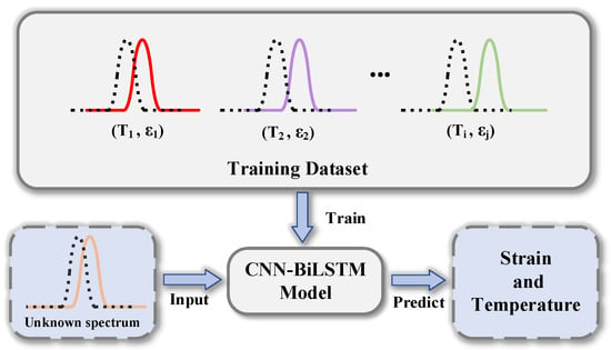
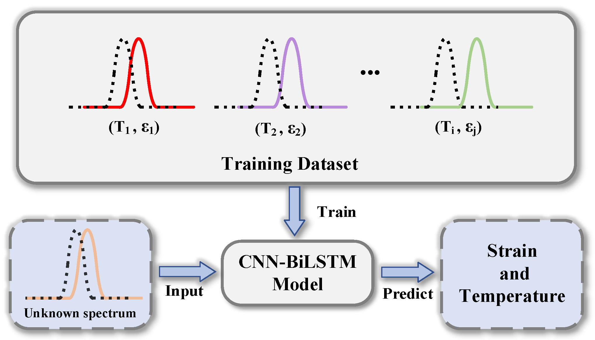
When external perturbations like ambient temperature and strain have changed, neff and Λ show corresponding variation, consequently inducing a shift in Bragg wavelength. The total wavelength shifts of the FBG peak are induced by the temperature and strain simultaneously. When the temperature and strain change simultaneously, the reflected spectrum shifts in the wavelength direction, as depicted in Figure 1. As shown in the figure, the reflection spectra and the corresponding parameters are taken as the training dataset. Subsequently, the unknown spectrum can be demodulated by the well-trained CNN-BiLSTM model. It is worth noting that the change in ambient temperature and strain can be calculated by the measured wavelength change of sensors through the sensitivity matrix. By converting the linear relationship between the wavelength shift and measurand to a matrix form, the sensitivity matrix could be deduced as follows [20]:
where ∆λB1 and ∆λB2 denote the relative peak wavelength shift of the reference FBG and sensing FBG, respectively. ΔT signifies the change in temperature, and Δε expresses the change in strain. KT1, Kε1, KT2, and Kε2 are the temperature sensitivity and strain sensitivity of the two FBGs. The scheme is easy to realize, but the sensitivity fluctuations in the application of the error brought about by the process cannot be avoided. Multi-parameter measurement based on SMM is heavily dependent on sensing sensitivity and measurement range. In other words, we have to balance the sensitivities among multi-parameters, which puts forward greater requirements on device design [11].
Figure 1.
Flow chart of FBG interrogation of strain and temperature sensing based on CNN-LSTM model. The black dashed spectrum is the original data. (Ti, εj) are different temperature and strain settings.
2.2. Design of the Demodulation System
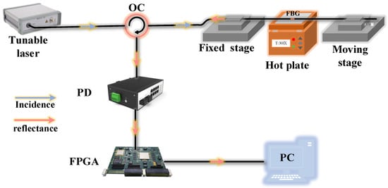
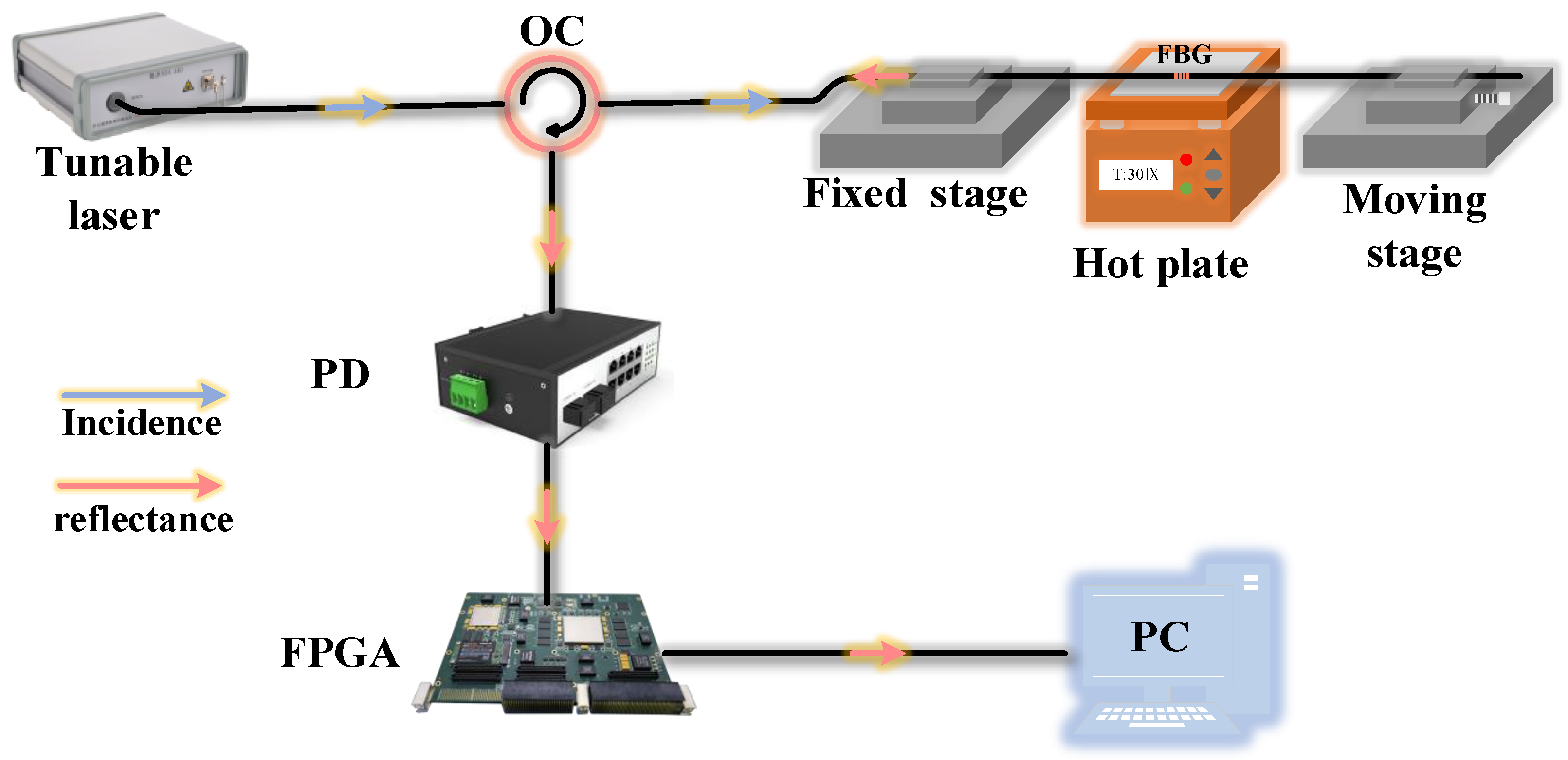
The experimental setup is illustrated in Figure 2. The sensor is placed on a precise heater to sense the testing temperature; meanwhile, the two ends of the sensor are fixed on a manual translation stage and a fixed translation stage by an optical adhesive to sense the applied strain. The distance between the two translation stages is 100 cm. The minimum achievable incremental movement of the manual translation stage is 0.01 mm. The manual translation stage moves a distance of 0.05 mm every time. Starting at 30 °C and ending at 120 °C, the heater was heated up at a step of 10 °C, and then a constant temperature was maintained for 5 min to collect the dataset. At any temperature, the number of strain measurements is 12, with a measurement range of 0–550 µε, and about 30 samples are collected for each strain case. Therefore, there are a total of 3621 sets of data, and the entire dataset was randomly partitioned into training, validation, and testing subsets at a ratio of 7:1:2. Based on the mechanics of materials, the strain (ε) measured by the FBG can be expressed as follows [21]:
where ∆L denotes the stretched length of the FBG, and L is the initial gauge length.
Figure 2.
Schematic diagram of the experimental setup for temperature and strain measurement. OC: optical circulator; PD: photodetector; FPGA: field programmable gate array; PC: personal computer.
The full spectrum consists of 5000 points, ranging from 1528 nm to 1568 nm. The light beam emitted from an MG-Y laser (AOC Technologies, Inc., Dublin, CA, USA) is guided into the FBG sensor probe via a circulator. Then, the reflected signals are detected by a photodetector (PD) (Thorlabs, Inc., Newton, NJ, USA). We used a field programmable gate array (FPGA) (Intel Corporation, Santa Clara, CA, USA) for precise wavelength control and simultaneous data acquisition [22]. The spectra of the sensor under different temperatures and strains are captured and recorded by a LabVIEW (2021 SP1) program. We acquired the spectrum by quasi-continuous wavelength scanning from 1568 nm to 1528 nm. For each wavelength output, the detected light intensity of the PD at that wavelength is collected. After completing one scan cycle, a complete spectrum can be acquired. The collected data is uploaded to a computer for the normalization operation to speed up model convergence and save training time. And then the spectral data and the corresponding targets (strain and temperature) will be fed into the model training as a dataset.
3. Neural Network Architecture
3.1. Convolutional Neural Networks
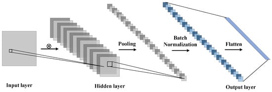
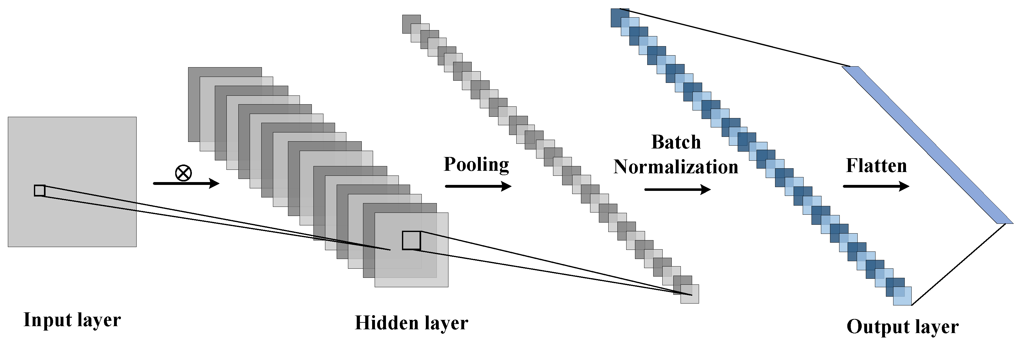
Serving as powerful feature extractors, convolutional neural networks (CNNs) are adept at mapping raw sequential inputs into hierarchical representations without requiring manual feature engineering [23]. Rather than adopting traditional 2D convolutions tailored for image processing, our framework utilizes 1D convolutional layers designed specifically to scan the spectral intensity distributed sequentially along the wavelength axis. Generally, a CNN model is composed of an input layer, a hidden layer, and an output layer, as shown in Figure 3. The original spectra working as the input layer are sent to the networks directly. The hidden layer mainly contains the convolutional layer, pooling layer, batch normalization (BN) layer and fully connected layer. The convolutional layer is used to extract feature maps from the original spectra by expanding the original single-channel data to multi-channel ones so as to extract spectral features from higher dimensions. The pooling layer is typically used between the convolutional layers to compress data and parameter volumes as well as to prevent overfitting. The BN layer [24] is used to normalize the data that will be transmitted to the next layer, which speeds up the training process and prevents overfitting.
Figure 3.
Schematic diagram of convolutional neural networks.
Since the FBG spectrum is a series of 1D signals, the convolutional layer we used in the model is a 1D temporal convolutional layer rather than its traditional 2D counterpart. The 1D convolutional operation used to extract the feature of the spectrum is formulated as follows:
where ⋆ is the valid cross-correlation operator, N is the batch size, C denotes the number of channels, and L is the length of the signal sequence.
3.2. Configuration of LSTM Memory Block
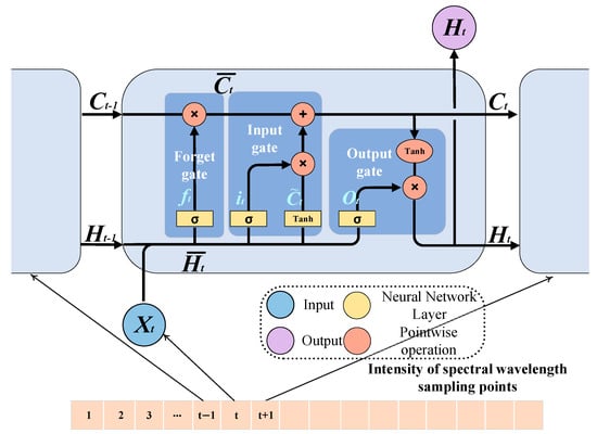
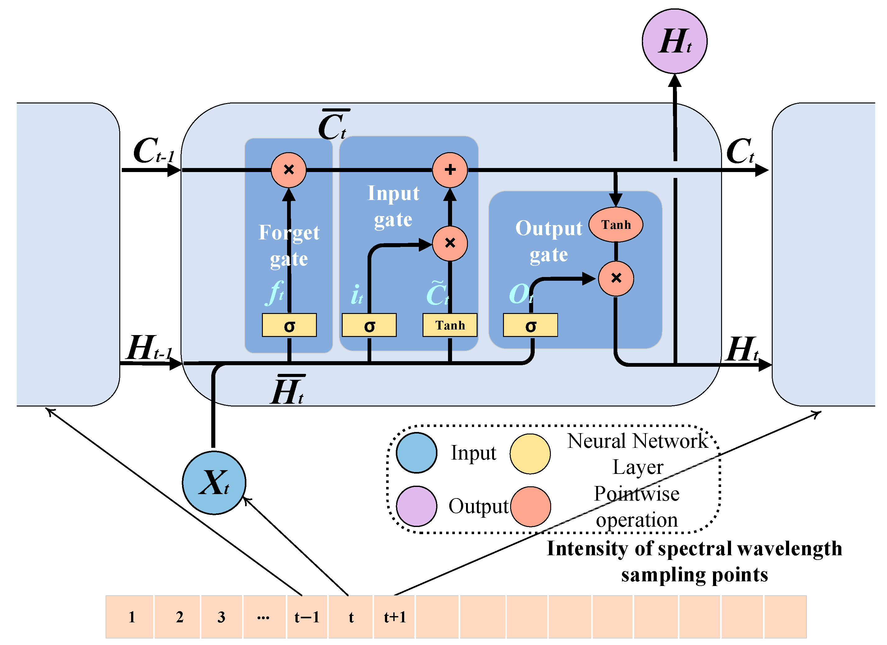
A standard LSTM architecture, as shown in Figure 4, circumvents the vanishing gradient problem found in basic RNNs by introducing a sophisticated memory cell state controlled by three interactive gating mechanisms: the forget gate, the input gate, and the output gate. Instead of merely overwriting data, the memory block evaluates the incoming spectral intensity at the current wavelength point (Xt) alongside the hidden state from the preceding wavelength (Ht−1). Specifically, the forget gate determines the proportion of previous spatial context (Ct−1) to retain, while the input gate regulates the incorporation of newly extracted features into the updated cell state (Ct). Finally, the output gate generates the subsequent hidden state (Ht), ensuring that long-range spatial dependencies across the Bragg peak are effectively preserved [25].
Figure 4.
Schematic structure of LSTM memory block.
The forgetting gate determines the degree of information to be retained in the previous sequence (Ct−1) through this value. It can be formulated as follows:
The process of the input gate can be described by the following equations:
The output gate is used to calculate the output, Ht, which is also the value of the next hidden layer. The process can be formulated as follows:
LSTM is able to capture long-term dependencies, which is useful for analyzing potential long-term patterns or trends in spectral data. The network is also capable of extracting dynamic features in spectra that are constantly changing over time, such as signal intensity, frequency, and energy distribution. It is critical to note that while an optical spectrum represents a static spatial frequency distribution rather than a temporal evolution, it is digitally acquired as an ordered sequence of intensity points across the wavelength axis. In this context, the memory parts within the BiLSTM are utilized to model the spatial correlations across the entire wavelength range. When an FBG is subjected to coupled temperature and strain, the cross-sensitivity induces not only a linear wavelength shift but also subtle physical deformations in the spectral profile, such as varying degrees of asymmetry or intensity fluctuations in the side lobes. BiLSTM allows the network to maintain the spatial context of the entire Bragg peak profile, extracting these distributed shape features collectively rather than treating each intensity point as an isolated data point. There are two LSTM layers in the bidirectional LSTM (BiLSTM) structure, one processing sequences from front to back and the other processing sequences from back to front. In this way, the model can utilize both front and back contextual information. While processing the sequence, the inputs of each time step are passed to each of the two LSTM layers, and then their outputs are merged. With BiLSTM, we can obtain more comprehensive information about the sequence, which helps to improve the performance of the model in the sequence task.
3.3. Configuration of the Proposed CNN-BiLSTM Model
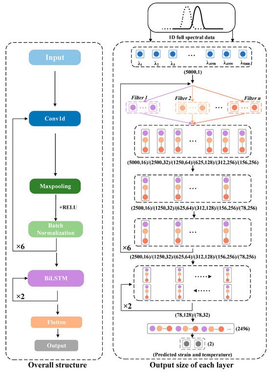
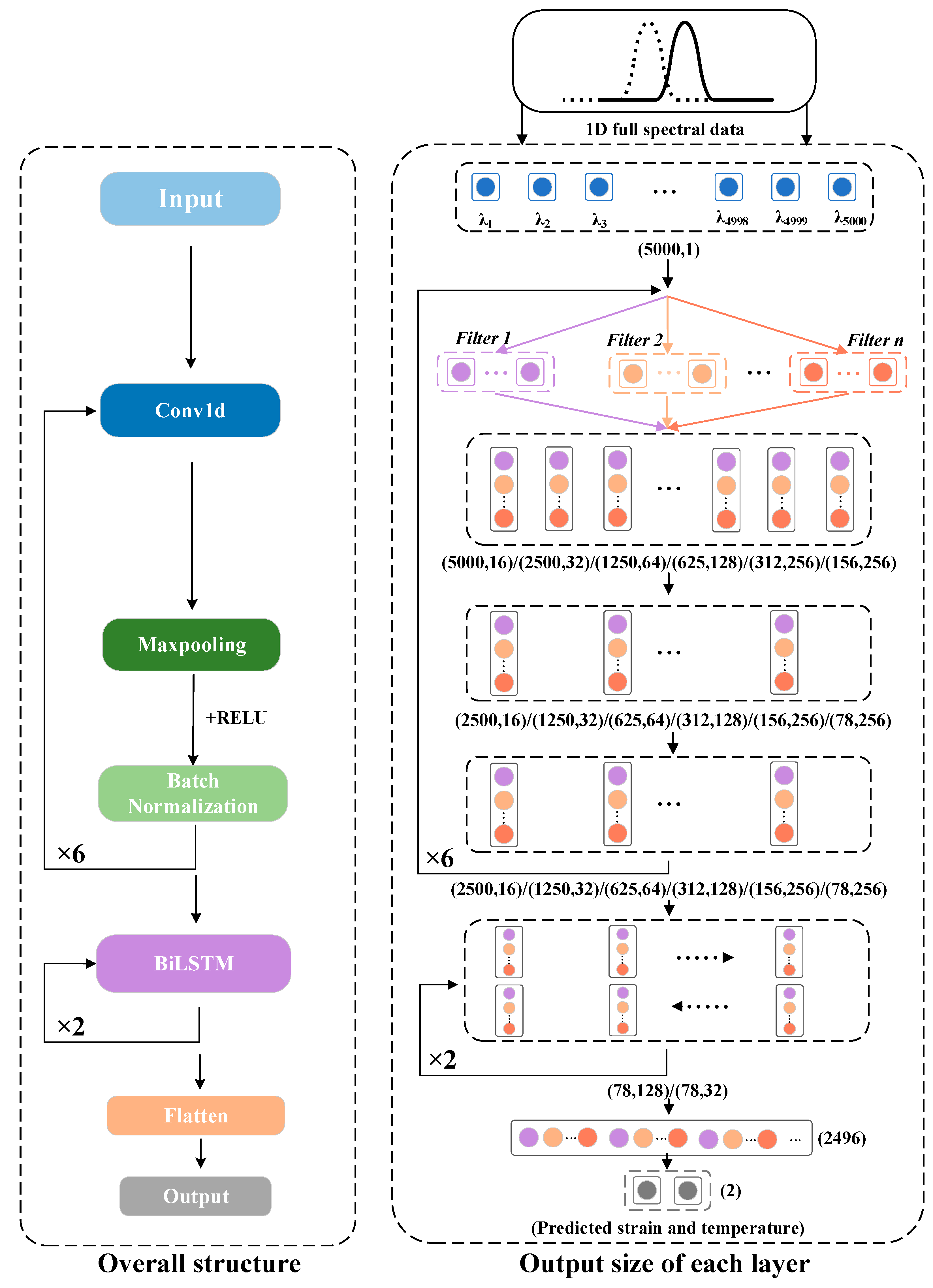
The CNN-BiLSTM model is a combination of two neural networks that takes full advantage of their strengths. It can mine the internal information of data from both spatial and sequential perspectives. Figure 5 illustrates the configuration of the proposed spectral demodulation model based on CNN-BiLSTM. There are six convolutional blocks after the input layer, each with a convolutional layer, a max-pooling layer, and a BN layer. The kernel size of the convolutional layer is 3, and the number of filters in these convolutional layers is 16, 32, 64, 128, 256 and 256, respectively. A max-pooling layer with a kernel size equal to 2 is used to reduce the data size to half. The BN layer is used to normalize the data that will be transmitted to the next layer. Then, the data is passed through two layers of BiLSTMs, which will train two LSTMs on the sequence [26]. The second LSTM is a reversed copy of the first one, so that we can take full advantage of both past and future input features for a specific time step. The hidden size of the two BiLSTM layers is 64, 16. The transformed data is then sent to a flattened layer to concatenate the dense layer as the output layer with a linear activation function. Finally, the model outputs the predicted strain and temperature.
Figure 5.
Proposed demodulation model based on CNN-BiLSTM for spectra. The arrows indicate the data flow paths, where turning arrows denote the repeated stacking of the corresponding modules.
The mean squared error (MSE) and coefficient of determination (R2) are used as the loss and criteria function in the training process, which can be formulated as follows:
where n is the number of spectral samples, and , , and are the true, predicted, and mean of the true values, respectively. The smaller the MSE is, the better the performance will be. The closer R2 is to approaching 1, the better the model is at identifying spectra. During the test, the root mean square error (RMSE) is used to judge the difference between the predicted result and the corresponding actual strain. The smaller the RMSE, the closer the predicted strain value is to the true strain. It can be expressed as follows:
For the network training dynamics, we selected the Adam optimizer [27] initialized with a learning rate of 0.001. To facilitate optimal convergence, a dynamic learning rate decay strategy (ReduceLROnPlateau) was implemented [28], which iteratively reduces the learning rate by a factor of 10 if the loss plateaus for 10 consecutive epochs. An early-stopping mechanism was also triggered to halt training and preserve the optimal model weights if no validation improvement was observed over 20 epochs, effectively preventing overfitting. The model was trained and verified in a Python 3.10 environment with Pytorch-GPU in a computer equipped with 12th Gen Intel(R) Core(TM)i7-12700H CPU @ 2.30 GHz, NVIDIA GeForce RTX 3060, and 6 GB.
It is worth noting that different temperature and strain conditions correspond to different spectra. The CNN-BiLSTM model extracts the features therein, learns the laws, and then establishes the connection between the spectra and the external parameters. Since we have enough sample data, the CNN-BiLSTM model is able to extract the spectral features under different temperature and strain conditions from both spatial and temporal perspectives, so as to distinguish the response of these two parameters to the spectra, which makes it possible to avoid the problem of cross-sensitivity.
4. Experimental Results
4.1. Strain and Temperature Demodulation
We first recorded the training and validation process by taking the average MSE of both strain and temperature as loss and the average R2 as accuracy. Then we studied them on the test set and analyzed the factors that may affect the prediction accuracy.
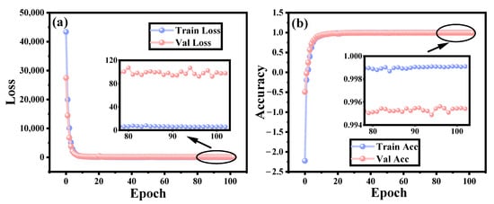
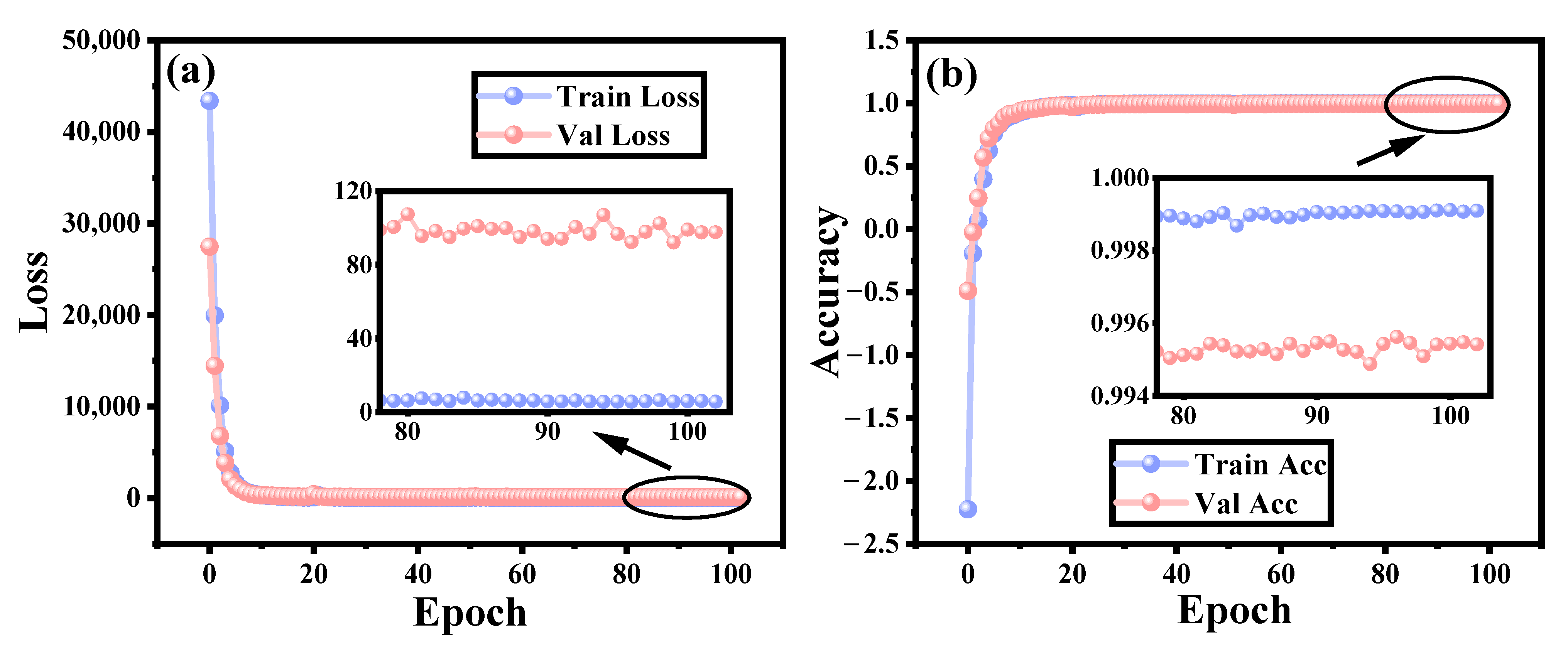
Figure 6a,b plot the loss and accuracy curve during the training of the proposed CNN-BiLSTM model using full spectral data. As a result, the model converges to constant after a few epochs, indicating that the model has learned the mapping relationship between the input spectrum and its corresponding strain and temperature. At the last 20 epochs, the curves of the training and validation fluctuate slightly, and no better performance is achieved during this interval. Then, the training process stopped at the 103rd epoch. The parameters of the epoch with the best performance were saved and used for the test process later on.
Figure 6.
(a) Loss and (b) accuracy variation during the training process of the proposed CNN-BiLSTM model.
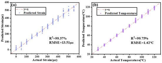
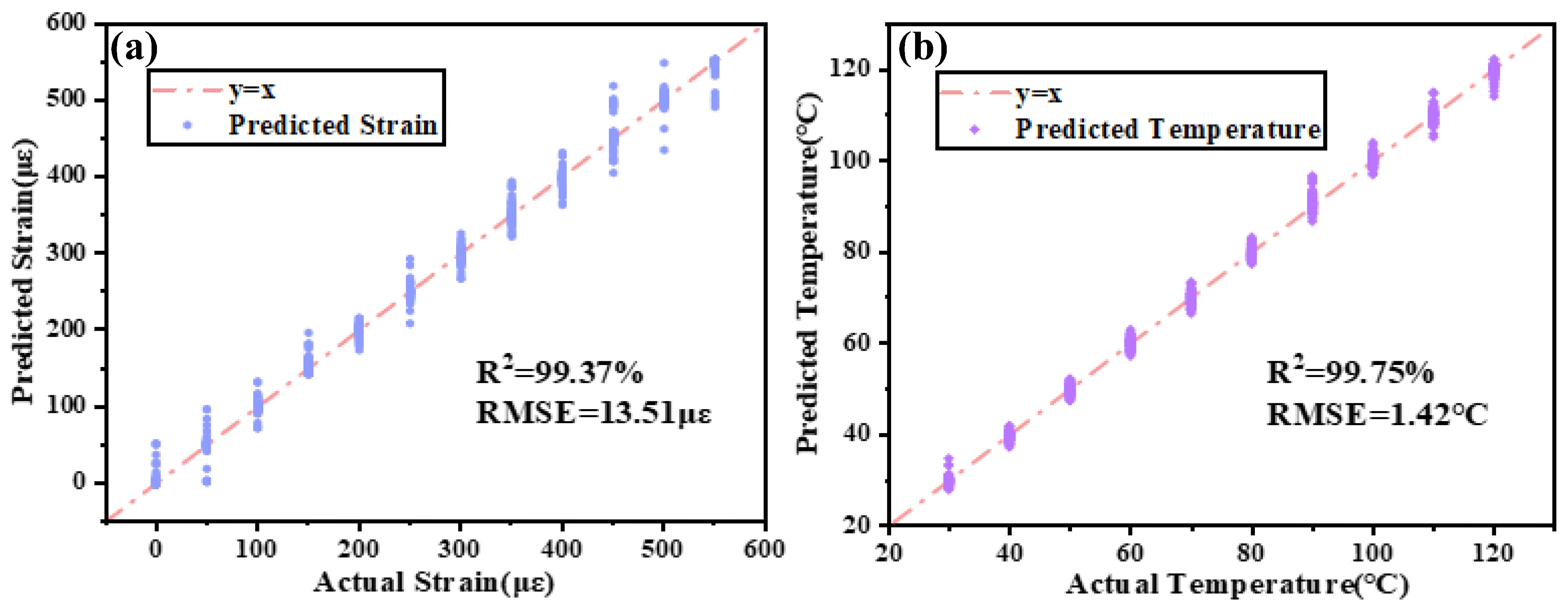
To explore the ability of the trained model, it is necessary to test it with some spectra that do not appear in the model training process. Figure 7a shows the strain prediction results of the model on test sets. In the figure, the red dashed line indicates that the predicted results are the same as the actual strain. The closer the predicted result is to the dashed line, the better the fitting effect. The blue dots represent the predicted results of the CNN-BiLSTM model. We can notice that the dots are concentrated near the straight line. The calculated R2 is 99.37%, and the RMSE is 13.51 µε, which shows that the model can exhibit good prediction performance for strain values.
Figure 7.
CNN-BiLSTM model prediction performance on test set. (a) Strain prediction results. (b) Temperature prediction results.
As shown in Figure 7b, the horizontal axis shows the actual temperature of the FBG sensor, and the vertical axis shows the temperature estimated using the CNN-BiLSTM model. We can observe that the predicted temperature values are more concentrated on the red straight line, indicating that the model performs better in predicting temperature compared to strain. The prediction error of RMSE is only 1.42 °C, and the R2 value of the model is reaching 99.75%. These values indicate the strong regression fitting performance of the model and further demonstrate the good generalization and robustness of the proposed model. The testing time for 720 testing samples is 1.05 s, implying that the information extraction for each spectrum takes only 1.46 ms, which is expected to realize real-time demodulation with guaranteed accuracy.
Next, we discuss the factors that may affect the demodulation accuracy of the scheme. They were analyzed from the perspective of the size of the dataset as well as the points of features, respectively. The experimental results are shown in Table 1. It is easy to find that when the size of the dataset is reduced, the accuracy decreases, which means that we need to spend time to collect enough datasets in advance. Second, the model demonstrates a clear sensitivity to the number of input spectral points. As shown in Table 1, reducing the spectral resolution from 5000 to 1000 points causes only a moderate increase in RMSE (from 13.51 µε and 1.42 °C to 18.36 µε and 2.57 °C). However, when the input points are further reduced to 200, the model’s accuracy begins to decrease significantly, with the strain RMSE more than doubling to 29.79 µε. This suggests that while the model can tolerate a certain degree of down-sampling, extreme feature reduction prevents the network from extracting sufficient spectral shape details to map the parameters accurately. Therefore, this places a specific requirement on the sampling rate of the spectrometer. For practical low-resolution scenarios where high-density sampling is unavailable, optimization strategies [2,25] would be necessary.
Table 1.
Analysis of factors affecting accuracy.
Furthermore, as a data-driven approach, the generalization ability of the CNN-BiLSTM model heavily relies on the scale of the training data. As shown in Table 1, reducing the dataset to 402 samples causes a notable drop in R2 for strain (from 99.37% to 96.41%), indicating that insufficient data restricts the model from learning the generalized physical mapping, which may lead to overfitting. Therefore, constructing a comprehensive dataset and maintaining sufficient spectral resolution are strictly necessary to ensure the model’s robustness and generalization in practical applications.
4.2. Comparison of SMMs and Different Machine Learning/Deep Learning Methods
A comparative table was developed to emphasize the performance of our proposed CNN-BiLSTM model, relative to SMMs and a series of algorithms. For each machine learning algorithm, we all carried out the 10-fold cross-validation in an attempt to fully display the performance of the proposed model. The entire dataset was randomly divided into 10 equal parts, one of which was selected without repetition as the test dataset and the rest was used as the training dataset. We took their average values for comparison, and the RMSE results for strain and temperature are shown in Table 2. We can see that the employment of the CNN-BiLSTM-based interrogation technique achieved RMSEs in the measurement of strain and temperature of 13.08 µε and 1.44 °C, respectively. In comparison with SMMs, the RMSE values decreased by 3~7 times and 4~15 times for the strain and temperature measurement, respectively.
Table 2.
RMSEs of strain and temperature prediction using sensitivity matrix methods and machine learning/deep learning methods.
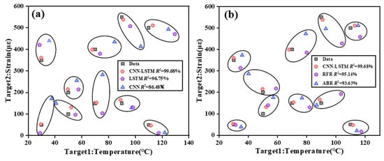
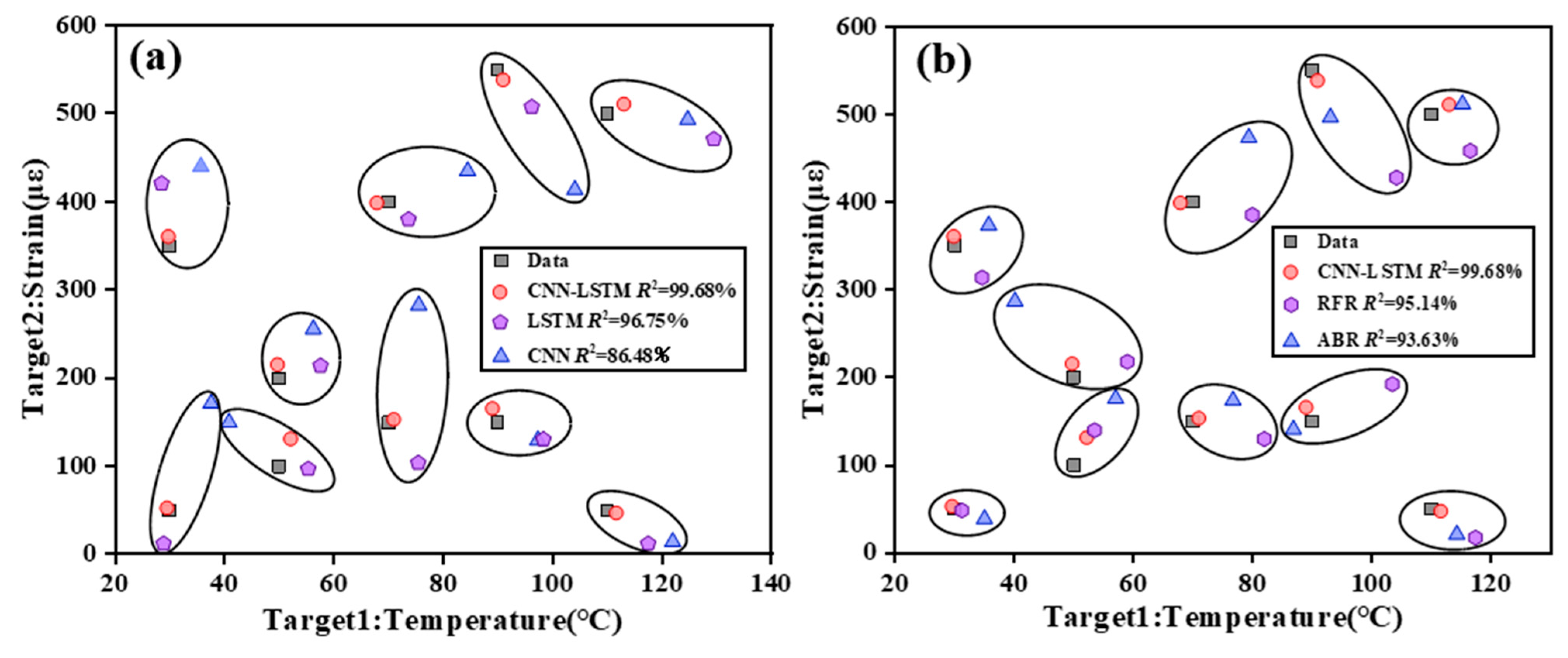
Random forest regressor and AdaBoost regressor are learning methods based on the Ensemble method, which fuses multiple models into a single learning model. Random forest regressor is classified as an Averaging method that can reduce variance, whereas AdaBoost regressor is classified as a Boosting method that can reduce bias. Figure 8 shows the predicted and targeted strain and temperature values using deep learning methods and two ensemble methods with their R2. As shown in the figure, the horizontal and vertical coordinates are temperature and strain, respectively. The black square is the true value, and the closer to it, the higher the accuracy. Obviously, the red circle, that is, our proposed CNN-BiLSTM model, has the highest demodulation accuracy of 99.68%. The above results indicate that the proposed model has excellent predictive ability and stability for both temperature and strain. And to a large extent, it alleviates the problem of cross-sensitivity between strain and temperature. Consequently, these qualities ensure the stability and precision of strain and temperature.
Figure 8.
Comparison of prediction performance between CNN-BiLSTM structure and other models. (a) Deep learning models. (b) Machine learning models. RFR: random forest regressor, ABR: AdaBoost regressor.
The CNN and BiLSTM networks have powerful capabilities in extracting spatial and temporal features of the input. CNN is able to capture local features, while BiLSTM is able to capture global and long-term-dependent features, which makes it able to extract the information in the sequence in a more comprehensive way. Therefore, the CNN-BiLSTM model has better performance in time series prediction tasks, which can better process the sequence data and improve the ability of the model to capture the important information in the sequence. However, it is worth mentioning that compared to some machine learning models, the training time increases as the depth of the model and the number of weights increase, which will result in increased training costs.
4.3. Temperature Compensation Methods with Two FBGs
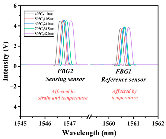
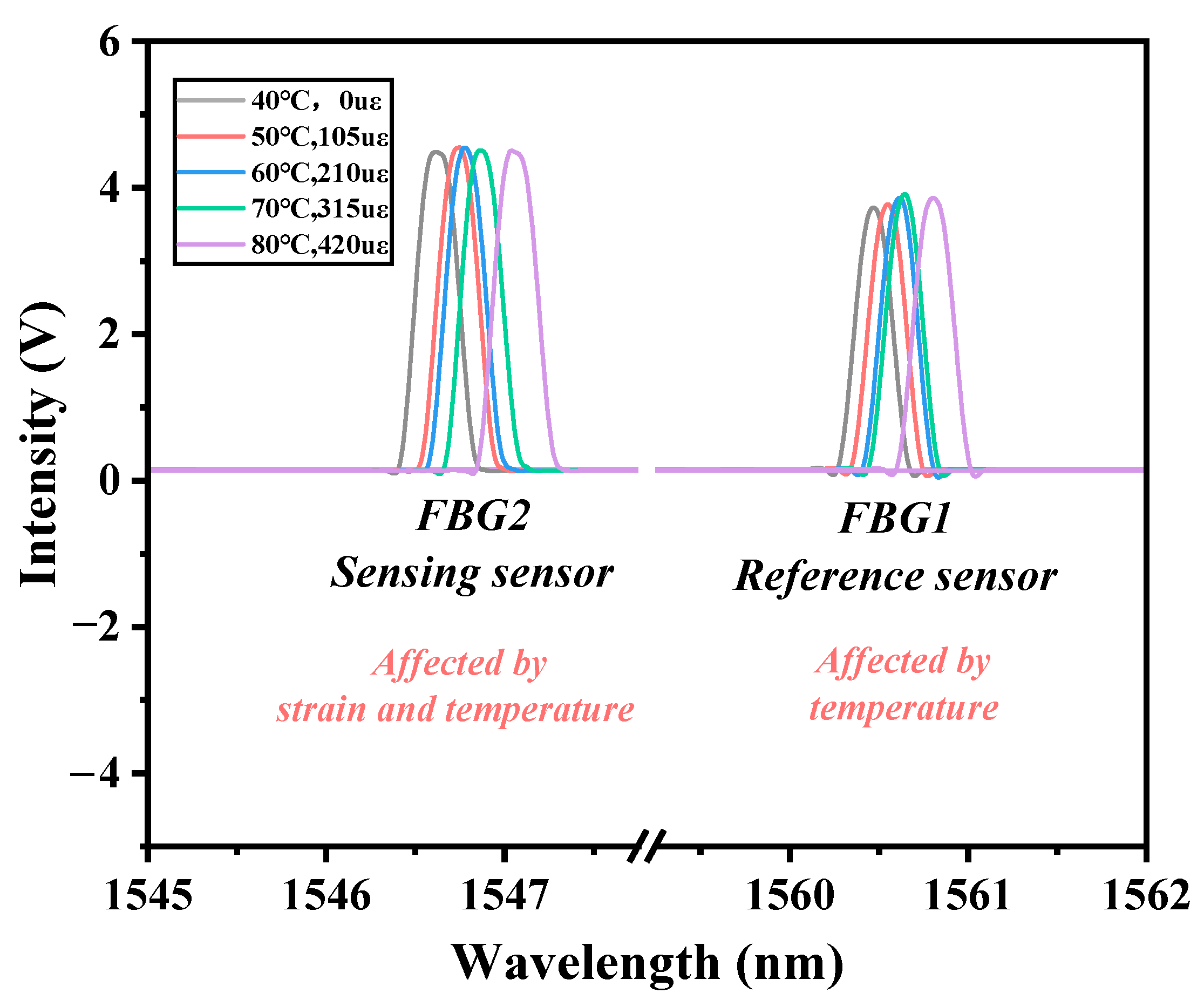
In certain special environments, specific temperature information cannot be obtained, thus making it impossible to collect a corresponding dataset for the aforementioned scheme. To address this issue, we utilized an additional reference fiber Bragg grating (FBG) to assist in temperature compensation. Their spectra are shown in Figure 9. The temperature sensitivity of the reference FBG was measured to be 8.82 pm/°C, and the temperature and strain sensitivities of the sensing FBG were 8.92 pm/°C and 0.45 pm/µε, respectively. Therefore, Equation (2) can be turned into the following form:
Figure 9.
Spectra of reference sensor FBG1 and sensing sensor FBG2.
Obviously, we can achieve temperature compensation by tracking the peak shift of the two sensors. The strain error calculated using this scheme is 57.8 µε. The main reason for the huge error is that SMM is not suitable for regions with poor sensitivity linearity. Secondly, the peaking tracing method cannot accurately find peaks because of system noise or sampling rates, thus leading to significant errors.
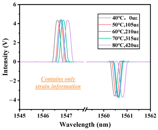
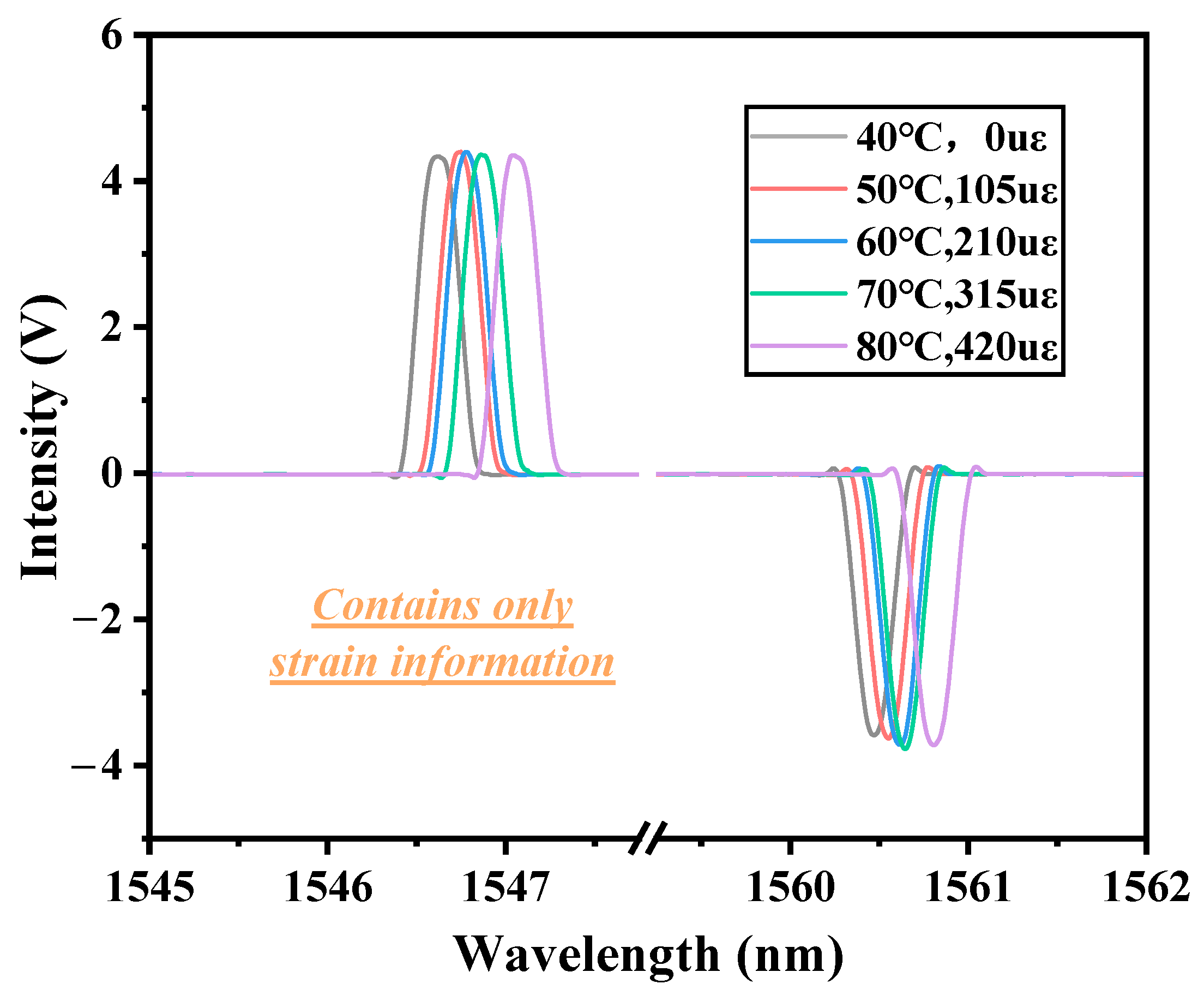
Therefore, we propose a spectral differencing method (SDM) to solve the above problem. We innovatively utilized the subtracted spectral difference between the two FBGs as the input dataset (as illustrated in Figure 10) to establish a direct mapping to the strain information. The reference sensor FBG1 contains only temperature information, while FBG2 contains both temperature and strain information. And they have almost the same sensitivity to temperature, so the differential spectrum can be considered to contain only strain. Then we feed the spectra into CNN-BiLSTM and let the model learn the connection between the spectra and the corresponding strain to get the predicted value. The RMSE on the test set is 14.98 µε, a decrease of almost 4 times compared to SMM. It should be noted that the precision of SDM is fundamentally constrained by the consistency of the temperature sensitivities between the two FBGs. In our experimental setup, the 0.1 pm/°C discrepancy (8.92 vs. 8.82 pm/°C) introduces a residual temperature-induced shift in the different spectra. Over the 90 °C testing range, this discrepancy generates a maximum residual shift of 9 pm, which translates to a theoretical maximum strain error of approximately 20 µε (given a strain sensitivity of 0.45 pm/µε). The achieved experimental RMSE of 14.98 µε accurately reflects this uncompensated residual error. While SDM bypasses the severe errors caused by the nonlinear sensitivity regions in traditional SMM, deploying this method in practical environments with extreme temperature fluctuations necessitates the careful physical pairing of FBGs with highly matched sensitivities to further minimize this residual crosstalk. This is attributed to the nonlinear fitting property of the deep learning model, which still finds the relationship between spectra and strain in the nonlinear sensitivity region where the sensitivity matrix method is not applicable. This solution does not need to measure the ambient temperature or the sensitivity of sensors in advance, which makes it suitable for more scenarios and even some complex environments.
Figure 10.
Spectra of FBG2 after differencing from FBG1.
4.4. Distributed FBG Sensing
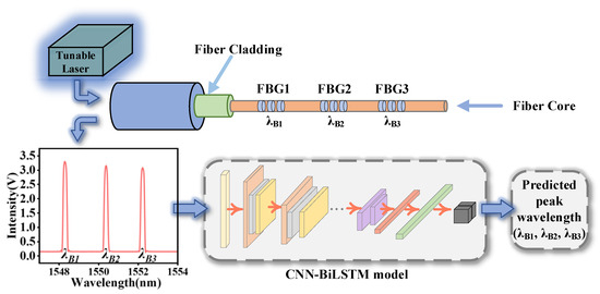
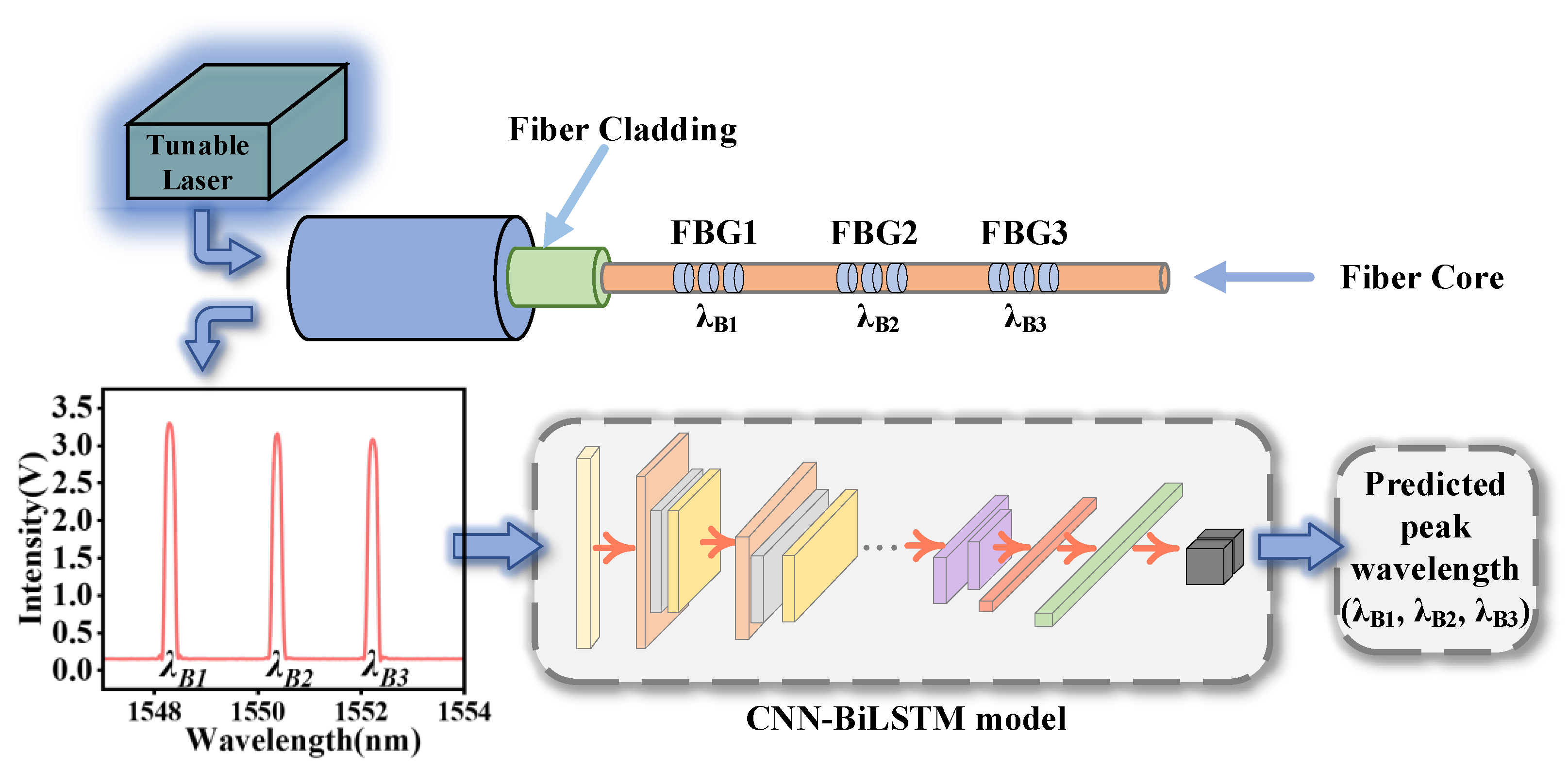
Finally, we explored the application of the system for distributed FBG sensors. This experiment was carried out using the experimental setup depicted in Figure 11 and the FBG array sensor, which consists of three FBGs. The center wavelength of them is approximately 1548 nm, 1550 nm and 1552 nm. During the experiments, a manual displacement stage was used to control the stretch relaxation of the FBG array sensors to acquire spectral data. The range of strain was from 0 to 525 µε, and we collected about 400 samples containing 16 strain cases. Since the initial center wavelengths of the three FBGs are sufficiently separated (1548 nm, 1550 nm, and 1552 nm) and the maximum applied strain of 525 µε induces a shift of only ~0.6 nm, spectral overlapping and physical crosstalk are effectively avoided in our current setup. Furthermore, unlike traditional peak-tracking algorithms whose computational complexity scales with the number of FBGs, our model processes the entire 5000-point composite spectrum as a single input vector. This ensures the inference time remains highly stable, highlighting its computational efficiency for real-time multi-point monitoring. However, deploying this architecture in dense arrays with severe spectral overlap and non-uniform power distribution remains a complex physical challenge that requires further investigation.
Figure 11.
Architecture of the FBG array sensor demodulation system and the spectrum of FBG array.
Since several peak wavelengths are the desired outcome, a multi-objective loss function was utilized, which may be written as Equation (15).
where n is the total number of samples; λ1, λ2 and λ3 represent the actual peak wavelengths of the peaks derived from OSA, respectively; and , and are the predicted values of the training model. The overall analysis of the demodulation performance of the CNN-BiLSTM model also used RMSE as a metric.
Experiments show that the proposed system can achieve at least ±0.02 nm of multi-peak absolute wavelength interrogation precision. The demodulation system provides an efficient and reliable solution for multi-point monitoring of large structures based on FBG array sensors.
5. Discussion
To evaluate the pioneering significance of the proposed CNN-BiLSTM architecture, it is essential to contextualize our findings within the landscape of existing decoupling methodologies. As evidenced by the comparative evaluation (detailed in Table 2), traditional SMMs frequently suffer from significant strain errors (e.g., 32 µε in [29] and 44 µε in [30]) due to their inability to dynamically adapt to the nonlinear cross-sensitivity variations inherent in varying thermal environments. While recent single-architecture machine learning approaches, such as standalone CNNs [23] or basic RNNs, have mitigated these linear limitations, they typically struggle to simultaneously capture both local geometric deformations and global sequence dependencies of the spectra.
Our work achieves a breakthrough by treating the optical spectrum as a spatial sequence. By integrating the local feature extraction capability of CNNs with the global spatial-context memory of BiLSTMs, the proposed model drastically reduces the RMSE to 13.08 µε for strain and 1.44 °C for temperature. This represents a substantial improvement over existing ensemble methods (like Random forest and AdaBoost), proving that hybridized deep learning structures offer a superior paradigm for decoupling highly correlated multi-parameter optical signals without relying on complex hardware modifications.
Due to inherent manufacturing tolerances (such as minor variations in doping concentration, grating period, and apodization profiles), no two FBGs possess identical baseline spectra or sensitivity matrices. Consequently, a model trained on a specific FBG inherently captures both the general physical laws of thermo-optic/elasto-optic coupling and the specific physical artifacts of that individual device. Therefore, applying this trained model directly to a newly fabricated, unseen FBG would likely result in baseline offsets. In practical deployments, the network architecture remains universal, but the parameters are sensor-specific. Utilizing transfer learning to fine-tune the pre-trained model with a smaller dataset from the new sensor is a highly viable solution to minimize this calibration burden.
Furthermore, the generalization ability of the network is bounded by the distribution of the training data. The model excels at interpolation within the calibrated parameter space (30–120 °C and 0–550 µε). However, its extrapolation capabilities are inherently limited. If the operating environment changes significantly, such as the temperature exceeding the calibration limit, or a severe strain gradient that causes spectral chirps (broadening and splitting) is introduced, the model will encounter spectral deformations it has not learned, leading to a decrease in prediction accuracy. Expanding the boundaries of the training dataset is necessary to deploy the system in more extreme operational environments.
For future industrial deployment in resource-constrained embedded systems (e.g., ARM microcontrollers or edge FPGAs), techniques such as model compression and lightweighting will be investigated to further reduce memory and power consumption while maintaining real-time monitoring capabilities.
6. Conclusions
To summarize, our experimental validation confirms that the hybridized CNN-BiLSTM architecture significantly elevates the precision of dual-parameter (temperature and strain) decoupling using merely a single FBG element. This data-driven approach distinctly outperforms conventional linear matrix techniques and standalone machine learning models by capturing the hidden spatial–sequential features of the entire spectrum. In addition, we proposed an SDM to address the problem of huge errors caused by nonlinear sensitivity in SMM. This proposed technique further could be expanded to interrogate a large number of FBGs to monitor structural health conditions and for distributed sensing purposes that are cost-effective and high-performance.
Author Contributions
Conceptualization, C.W. and Q.L.; sensor fabrication, C.W. and D.L.; software, Q.L.; validation, J.S. and D.Z.; investigation, C.W.; writing—original draft preparation, C.W.; writing—review and editing, Q.L.; supervision, Y.W.; project administration, Q.L. All authors have read and agreed to the published version of the manuscript.
Funding
This work was supported in part by the National Natural Science Foundation of China (62405139, 62575140 and 62505139).
Institutional Review Board Statement
Not applicable.
Informed Consent Statement
Informed consent was obtained from all subjects involved in the study.
Data Availability Statement
The dataset is available on request from the authors.
Conflicts of Interest
The authors declare no conflicts of interest.
References
- Leal-Junior, A.; Díaz, C.; Frizera, A.; Lee, H.; Nakamura, K.; Mizuno, Y.; Marques, C. Highly sensitive fiber-optic intrinsic electromagnetic field sensing. Adv. Photonics Res. 2021, 2, 2000078. [Google Scholar] [CrossRef] [Scilit]
- Wei, C.; Liu, Q.; Zhu, S.; Zhu, D.; Shi, J.; Lin, D.; Wang, Y. Deep learning enhanced fiber-optic Fabry–Perot sensor demodulation with sparse sampling points using GAF algorithm. IEEE Sens. J. 2024, 24, 26845–26852. [Google Scholar] [CrossRef] [Scilit]
- Burunkaya, M.; Yucel, M. Measurement and Control of an Incubator Temperature by Using Conventional Methods and Fiber Bragg Grating (FBG) Based Temperature Sensors. J. Med. Syst. 2020, 44, 178. [Google Scholar] [CrossRef] [Scilit]
- Li, L.; Wang, Y.; Zhu, D.; Tian, X.; Shi, J.; Gao, L.; Xiao, Y. Distributed strain interrogation with a linearly chirped fiber Bragg grating based on an optoelectronic oscillator. Appl. Opt. 2023, 62, 367. [Google Scholar] [CrossRef] [Scilit]
- Tian, X.; Shen, C.; Ma, D.; Huang, C.; Liu, Y.; Liang, L.; Wang, Y. Temperature-compensated Fiber Bragg Grating Strain Sensor Based on a Two-tap Microwave Photonic Filter. J. Light. Technol. 2023, 42, 2532–2537. [Google Scholar] [CrossRef] [Scilit]
- Xu, M.; Archambault, J.; Reekie, L.; Dakin, J. Discrimination between strain and temperature effect using dual wavelength fiber grating sensors. Electron. Lett. 1994, 30, 1085–1087. [Google Scholar] [CrossRef] [Scilit]
- Guan, B.; Tam, H.; Tao, X.; Dong, X. Simultaneous strain and temperature measurement using a superstructure fiber Bragg grating. IEEE Photonics Technol. Lett. 2000, 12, 675–677. [Google Scholar] [CrossRef] [Scilit]
- Su, D.; Qiao, X.; Chen, F.; Bao, W. Compact dual fiber Bragg gratings for simultaneous strain and high-temperature measurement. IEEE Sens. J. 2019, 19, 5660–5664. [Google Scholar] [CrossRef] [Scilit]
- Leng, J.; Asundi, A. Real-time cure monitoring of smart composite materials using extrinsic Fabry-Perot interferometer and fiber Bragg grating sensors. Smart Mater. Struct. 2002, 11, 249–255. [Google Scholar] [CrossRef] [Scilit]
- Kipriksiz, S.E.; Yücel, M. Tilted fiber Bragg grating design for a simultaneous measurement of temperature and strain. Opt. Quantum Electron. 2021, 53, 6. [Google Scholar] [CrossRef] [Scilit]
- Liu, J.; Hou, Y.; Wang, J.; Zhong, G.; Zhang, L.; Zhuang, F.; Yu, L.; Wang, S. Multi-parameter demodulation for temperature, salinity and pressure sensor in seawater based on the semi-encapsulated microfiber Mach-Zehnder interferometer. Measurement 2022, 196, 111213. [Google Scholar] [CrossRef] [Scilit]
- Djurhuus, M.S.E.; Werzinger, S.; Schmauss, B.; Clausen, A.T.; Zibar, D. Machine learning assisted fiber bragg grating-based temperature sensing. Photonics Technol. Lett. 2019, 31, 939–942. [Google Scholar] [CrossRef] [Scilit]
- Sarkar, S.; Inupakutika, D.; Banerjee, M.; Tarhani, M.; Shadaram, M. Machine learning methods for discriminating strain and temperature effects on FBG-based sensors. Photonics Technol. Lett. 2021, 33, 876–879. [Google Scholar] [CrossRef] [Scilit]
- Kikuchi, M.; Ogasawara, T.; Fujii, S.; Takeda, S.-I. Application of machine learning for improved accuracy of simultaneous temperature and strain measurements of carbon fiber-reinforced plastic laminates using an embedded tilted fiber Bragg grating sensor. Compos. Part A Appl. Sci. Manuf. 2022, 161, 107108. [Google Scholar] [CrossRef] [Scilit]
- Mei, S.; Ji, J.; Hou, J.; Li, X.; Du, Q. Learning Sensor-Specific Spatial-Spectral Features of Hyperspectral Images via Convolutional Neural Networks. IEEE Trans. Geosci. Remote Sens. 2017, 55, 4520–4533. [Google Scholar] [CrossRef] [Scilit]
- Jiang, H.; Zeng, Q.; Chen, J.; Qiu, X.; Liu, X.; Chen, Z.; Miao, X. Wavelength detection of model-sharing fiber Bragg grating sensor networks using long short-term memory neural network. Opt. Express 2019, 27, 20583–20596. [Google Scholar] [CrossRef] [Scilit]
- Wang, Y.; Wan, S.; Zhang, S.; Yu, J. Speaker Recognition of Fiber-Optic External Fabry-Perot Interferometric Microphone Based on Deep Learning. IEEE Sens. J. 2022, 22, 12906–12912. [Google Scholar] [CrossRef] [Scilit]
- Mohammed, A.; Hu, B.; Hu, Z.; Djurovic, S.; Ran, L.; Barnes, M.; Mawby, P.A. Distributed thermal monitoring of wind turbine power electronic modules using FBG sensing technology. IEEE Sens. J. 2020, 20, 9886–9894. [Google Scholar] [CrossRef] [Scilit]
- Erdogan, T. Fiber grating spectra. J. Lightw. Technol. 1997, 15, 1277–1294. [Google Scholar] [CrossRef] [Scilit]
- Zhang, G.; Ge, Q.; Wang, H.; Wu, X.; Yu, B. Simultaneous temperature and strain measurement using TCF based Mach-Zehnder interferometer. Opt. Fiber Technol. 2021, 67, 102687. [Google Scholar] [CrossRef] [Scilit]
- Zhou, K.; Ai, M.Z.; Qian, Z.H.; Gao, X.X.; Hu, Z.H.; Li, Q.; Yuan, L.; Wang, Z.; Huang, Y.F.; Tu, T. High-sensitivity strain sensor with an in-fiber air-bubble Fabry-Perot interferometer. Appl. Phys. Lett. 2018, 113, 181901. [Google Scholar] [CrossRef] [Scilit]
- Liu, Q.; Jing, Z.; Li, A.; Liu, Y.; Huang, Z.; Zhang, Y.; Peng, W. Common-path dual-wavelength quadrature phase demodulation of EFPI sensors using a broadly tunable MG-Y laser. Opt. Express 2019, 27, 27873–27881. [Google Scholar] [CrossRef] [Scilit]
- Cao, Z.; Zhang, S.; Xia, T.; Liu, Z.; Li, Z. Spectral demodulation of fiber Bragg grating sensor based on deep convolutional neural networks. J. Light. Technol. 2022, 40, 4429–4435. [Google Scholar] [CrossRef] [Scilit]
- Ioffe, S.; Szegedy, C. Batch Normalization: Accelerating Deep Network Training by Reducing Internal Covariate Shift. Pr. Mach. Learn. Res. 2015, 37, 448–456. [Google Scholar]
- Mei, Y.; Zhang, S.; Cao, Z.; Xia, T.; Yi, X.; Liu, Z. Deep learning assisted pressure sensing based on Sagnac interferometry realized by side-hole fiber. J. Light. Technol. 2022, 41, 784–793. [Google Scholar] [CrossRef] [Scilit]
- Tavakoli, N. Modeling Genome Data Using Bidirectional LSTM. In Proceedings of the IEEE 43rd Annual Computer Software and Applications Conference (COMPSAC), Milwaukee, WI, USA, 15–19 July 2019; Volume 2, pp. 183–188. [Google Scholar]
- Kingma, D.; Ba, J. Adam: A method for stochastic optimization. Comput. Sci. arXiv 2014, arXiv:1412.6980. [Google Scholar]
- Ibrahim, Z.; Fahmy, Y. Enhanced learning for recurrent neural network-based polar decoder. In Proceedings of the 2022 13th International Conference on Electrical Engineering (ICEENG), Cairo, Egypt, 29–31 March 2022; pp. 105–109. [Google Scholar]
- Dey, K.; Nikhil, V.; Roy, S. Machine learning approach for simultaneous measurement of strain and temperature using FBG sensor. Sens. Actuators A Phys. 2022, 333, 113254. [Google Scholar] [CrossRef] [Scilit]
- Dey, K.; Nikhil, V.; Roy, S. Machine learning approach with higher accuracy for simultaneous measurement of the dual parameter by MSM fiber structure. Measurement 2023, 221, 113426. [Google Scholar] [CrossRef] [Scilit]

Disclaimer/Publisher’s Note: The statements, opinions and data contained in all publications are solely those of the individual author(s) and contributor(s) and not of MDPI and/or the editor(s). MDPI and/or the editor(s) disclaim responsibility for any injury to people or property resulting from any ideas, methods, instructions or products referred to in the content. |
© 2026 by the authors. Licensee MDPI, Basel, Switzerland. This article is an open access article distributed under the terms and conditions of the Creative Commons Attribution (CC BY) license.