Plane-Guided Point-Line LiDAR–Camera Extrinsic Calibration with Finite Line-Segment Constraints

Abstract

Light detection and ranging (LiDAR)–camera calibration requires reliable target reconstruction and robust pose estimation. We present P3LPnP, a plane-guided point-line framework that registers a known-size checkerboard lattice and jointly optimizes point re-projection and finite-segment length, direction, and endpoint position. The front end combines random sample consensus (RANSAC), density-based spatial clustering of applications with noise (DBSCAN), and principal component analysis (PCA). The back end uses iteratively re-weighted least squares with weights fixed during inner solves and exact-Huber step acceptance. In 30 matched synthetic scenes, P3LPnP achieved a plane root mean square error of 0.673 mm. Relative to point-only optimization, finite-segment constraints reduced mean clean-reference re-projection error from 0.441 to 0.399 pixels and translation error from 5.094 to 3.424 mm. Synthetic tests showed translation robustness to point noise and coherent bias, with competitive performance under sparse joint noise. A 30-run controlled replay from one system yielded mean re-projection errors of 0.356 and 0.338 pixels on 100 sparse reference points and 9900 same-session held-out points. Real-data evidence supported same-system consistency; the advantage over the point-line baseline was not statistically significant, and multi-system generalizability remained unverified.

1. Introduction

Light detection and ranging (LiDAR) and cameras provide complementary measurements: LiDAR supplies metric range information, whereas cameras provide dense appearance and texture. Accurate extrinsic calibration is therefore required to project LiDAR measurements into the image and to fuse the two modalities in a common coordinate system for perception and three-dimensional reconstruction [1,2,3,4,5,6,7]. Existing calibration methods commonly exploit designed targets, scene geometry, or motion, and they formulate the estimation problem using point, plane, line, or mixed geometric constraints [8,9].

Laser-scanning design also influences the spatial coverage and sampling pattern of LiDAR measurements. Lee et al. investigated optical scan-angle expansion in a microelectromechanical systems (MEMS)-based LiDAR system [10]. Duma and Dimb analyzed the exact scan patterns of rotational Risley prisms using a graphical method [11]. Li et al. developed a Risley-prism multi-beam LiDAR for high-resolution three-dimensional imaging [12], while Liu et al. studied cascaded-prism scanning to enable configurable imaging modes with different fields of view, angular resolutions, and sampling densities [13]. These studies provide the optical and sampling context for LiDAR-based 3D measurement. Against this background, reliable target-feature reconstruction and cross-modal registration remain necessary when the available calibration-board returns are sparse.

Point-based calibration is efficient when accurate and well-distributed 3D–2D correspondences are available, and modern perspective-n-point (PnP) solvers provide strong computational and numerical foundations for this setting [14,15,16]. In sparse-scanning LiDAR–camera calibration, however, an important difficulty occurs before pose estimation: limited angular sampling can leave only a small number of returns on the target, time-of-flight noise perturbs range measurements along the laser rays, and cross-modal feature localization can displace the reconstructed target points from their intended image features [17,18,19,20,21,22]. These effects reduce the amount or accuracy of the available correspondence information. Accordingly, the issue considered in this work is not that point-based pose estimation is intrinsically unreliable, but that correspondence construction and uncertainty propagation can become the limiting steps when the LiDAR observations are sparse or noisy [23].

Line features provide complementary structural information because an observed edge constrains a spatial extent rather than only an isolated location. Line-correspondence calibration and joint point-line pose estimation have therefore been studied for both sensor calibration and general camera pose recovery [22,24,25]. Most such formulations are built around a supporting-line incidence or algebraic point-to-line relation. This is appropriate for unbounded lines, but it does not by itself distinguish the information carried by the measured length, orientation, and endpoint locations of a finite calibration-board segment. Moreover, the reliability of these attributes is not uniform: random endpoint noise and systematic endpoint bias can affect a finite segment differently. A calibration formulation should therefore expose these contributions separately rather than treating every line observation as an undifferentiated constraint.

The accuracy of the back-end pose estimate also depends on the three-dimensional target reference supplied by the front end. A fitted plane determines the board orientation and a local in-plane basis, but it does not alone determine the translation and orientation of the checkerboard lattice within that plane. Previous work has therefore used ranging statistics, reflectance patterns, and full-scale target models to recover board features from sparse or non-uniform LiDAR returns [19,21,26]. For sparse and contaminated board returns, the plane, board boundary, and known-size grid must therefore be reconstructed as a coupled geometric reference before 3D–2D correspondences are passed to the pose solver. This observation motivates a framework in which target reconstruction and finite-segment pose constraints are designed and evaluated as linked, but separately auditable, components.

This paper presents P3LPnP, a plane-guided point-line framework for target-based LiDAR–camera extrinsic calibration under sparse and noisy ranging observations. The principal contributions are as follows:

• A calibration-oriented front end reconstructs a known-size rigid checkerboard lattice from sparse LiDAR returns. Its plane extraction, inlier purification, and grid-localization stages are explicitly described and individually evaluated, so that the origin of the reconstructed 3D corners is reproducible rather than being attributed to principal component analysis (PCA) alone.
• A robust point-line objective separates finite-segment length, direction, and endpoint-position residuals from the point re-projection residuals. The formulation and ablation protocol distinguish the geometric information contributed by each term from the effect of assigning extra weight to boundary correspondences.
• A matched evaluation protocol examined front-end reconstruction, line-term ablation, parameter sensitivity, point-observation noise, joint point–line localization noise, and coherent image-feature bias. Real-data results are reported as same-system sparse-to-dense consistency tests, and the limitation to one LiDAR–camera rig and one acquisition session is stated explicitly.

The remainder of this paper is organized as follows. Section 2 reviews target-based, line-based, point-line, and targetless calibration methods and identifies the scope addressed here. Section 3 presents the materials and methods. Section 4 describes the experimental protocol. Section 5 reports the results. Section 6 discusses the validation boundary and limitations. Section 7 concludes the paper.

2. Related Work

2.1. Target-Based Point and Plane Calibration

Point-based LiDAR–camera calibration estimates the extrinsic transformation from matched geometric features. General PnP solvers provide the relevant pose-estimation foundation: efficient perspective-n-point (EPnP) uses virtual control points for linear-complexity computation [14], the direct least-squares (DLS) method derives a pose solution [15], and the sequential quadratic programming PnP solver (SQPnP) provides a consistently fast globally optimal formulation [16]. More recent methods incorporate probabilistic modeling, robust estimation, or additional depth information [27,28,29]. Uncertainty-aware point-and-line pose-estimation work further shows that both the three-dimensional features and their image projections may carry non-negligible uncertainty [23].

For LiDAR–camera calibration, designed targets make the cross-modal geometry observable through corners, holes, planes, or other known structures. Representative methods use direct 3D–2D correspondences, virtual points, 3D–3D correspondences, planar targets, or single-shot target configurations [6,7,8,30,31,32]. Yi et al. used a laser detector card to establish direct correspondences between LiDAR laser points and image pixels [17], whereas Jeong et al. modeled LiDAR sampling and ranging characteristics in a one-shot, one-target setting [18]. These studies demonstrate that a point-based back end can be effective when target features are reconstructed reliably. They also show why the front end matters: sparse angular sampling, range uncertainty, and the difference between a physical boundary and the points returned near a depth discontinuity can bias the geometric features before PnP is applied [18].

Several studies have addressed target-reference recovery itself rather than assuming that accurate 3D target points are already available. Xu et al. used ranging statistics and an improved random sample consensus (RANSAC) procedure to filter low-resolution LiDAR returns and extract calibration features [19]. Wang et al. fitted a full-scale printed-checkerboard model to a sparse single-frame LiDAR point cloud by correlating the model pattern with LiDAR reflectance and optimizing the model pose [26]. Lai et al. likewise exploited laser reflectance features to handle the non-uniform density of non-repetitive scanning LiDAR [21]. These methods have established that board localization is a substantive part of calibration. The front end studied here occupies a narrower, geometry-only setting: it registers a known-size rigid lattice in the estimated plane without using LiDAR reflectance intensity, and it does not claim that PCA alone determines the grid pose.

2.2. Line-Based and Point-Line Calibration

Line features have been used to improve geometric coverage in structured environments and on calibration targets. General line-pose methods estimate camera pose from 3D–2D line correspondences [33,34], while LiDAR–camera methods use target edges, box structures, or indirect point-to-line correspondences [22,24,35,36]. Such constraints are attractive when individual corners are difficult to localize, but line-only geometry can have weak observability for particular motions or translations; combining points and lines can retain local anchoring while adding extended structural information.

Vakhitov et al. introduced an extension of optimal PnP to point and line correspondences, denoted OPnPL, which incorporates 3D–2D line correspondences into point-based PnP through algebraic constraints on the 3D line endpoints, including cases in which the corresponding 2D endpoints are not directly observed [25]. Later uncertainty-aware work incorporated uncertainty in both points and lines [23]. These formulations establish the value of point-line fusion, but their supporting-line constraints are conceptually different from explicitly comparing the measured endpoints and finite extent of a projected calibration-board segment. LiDAR–camera calibration studies likewise employ line incidence, point-to-line distance, or combined feature distances [22,24]. Across these formulations, the separate effects of finite-segment length, direction, and observed endpoint position under both random line noise and systematic line bias remain less explicit. This motivates a controlled decomposition of the line residuals, including a control that tests whether an endpoint term contributes information beyond simply re-weighting existing boundary points.

2.3. Targetless Calibration and Research Gap

Targetless methods avoid a dedicated calibration object by aligning scene edges, natural structures, intensity information, or motion-derived constraints. Existing approaches address unstructured environments, edge alignment, low-resolution LiDAR, roadside installations, and online or real-time operation [20,37,38,39,40,41]. These methods broaden the operational scope of LiDAR–camera calibration, but they commonly require sufficiently informative scene geometry, repeated observations, platform motion, or application-specific spatial and temporal assumptions. They are therefore complementary to, rather than direct substitutes for, a controlled target-based procedure intended for sparse board scans.

Prior work has thus addressed target design, LiDAR-specific sampling effects, full-scale or reflectance-assisted checkerboard fitting, point-line pose estimation, and targetless operation. The scope addressed here is therefore not the first use of a checkerboard model. Instead, two linked issues remain less completely exposed in a single sparse-scan target-based evaluation: geometry-only localization of a known rigid lattice within a robustly reconstructed plane, and separate auditing of finite-segment length, direction, and endpoint-position contributions after point correspondences are already present. P3LPnP addresses this bounded scope by coupling explicit target-reference reconstruction with decomposed finite-segment constraints. The processing sequence, residual definitions, robust optimization, and parameter settings are presented in Section 3.

3. Materials and Methods

3.1. Calibration Model and Notation

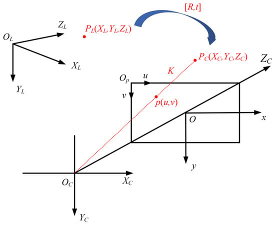
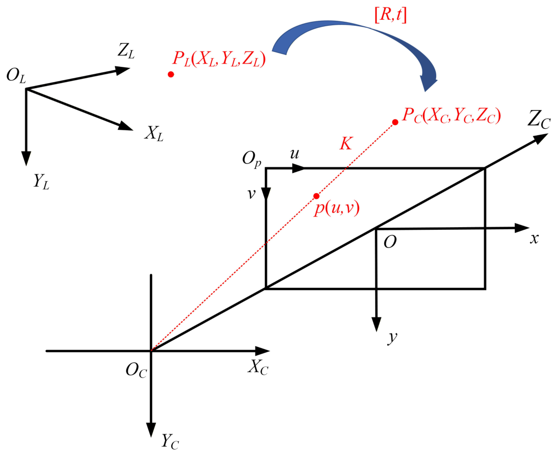
The goal of extrinsic calibration is to estimate the rigid transformation from the LiDAR frame $O_L-X_L{Y}_L{Z}_L$ to the camera frame $O_C-X_C{Y}_C{Z}_C$. The normalized image frame and the pixel frame are denoted as $O-xy$ and $O_p-uv$, respectively. The coordinate transformation chain is shown in Figure 1. Specifically, the projection from the camera coordinate frame onto the image plane is described by the pinhole camera model and is parameterized by the intrinsic matrix $\mathbf{K}$. The spatial transformation that aligns the LiDAR frame with the camera frame is defined by the extrinsic parameters $\left[\mathbf{R},\mathbf{t}\right]$, which encode the relative rotation and translation between the two sensors.

Figure 1. Coordinate transformation chain used in the light detection and ranging (LiDAR)–camera calibration model.

For a LiDAR point ${\mathbf{P}}_L={[X_L,Y_L,Z_L]}^T$, its camera-frame coordinate is

$${\mathbf{P}}_C={\left[\begin{array}{ccc}{X}_C& Y_C& Z_C\end{array}\right]}^T=\mathbf{R}{\mathbf{P}}_L+\mathbf{t},$$

(1)

where $\mathbf{R}\in SO\left(3\right)$ and $\mathbf{t}\in {\mathbb{R}}^3$ are the rotation and translation from ${\mathcal{F}}_L$ to ${\mathcal{F}}_C$. The pixel projection is

$$s\left[\begin{array}{c}u\\ v\\ 1\end{array}\right]=\mathbf{K}\left[\begin{array}{cc}\mathbf{R}& \mathbf{t}\end{array}\right]\left[\begin{array}{c}{\mathbf{P}}_L\\ 1\end{array}\right],\mathbf{K}=\left[\begin{array}{ccc}{f}_x& 0& u_0\\ 0& f_y& v_0\\ 0& 0& 1\end{array}\right],$$

(2)

where $\mathbf{K}$ is the intrinsic matrix and $s=Z_C$ is the projective scale. The projection function is written as

$$\widehat{\mathbf{p}}=\pi (\mathbf{R}{\mathbf{P}}_L+\mathbf{t}).$$

(3)

3.2. Plane-Guided Front-End Reconstruction

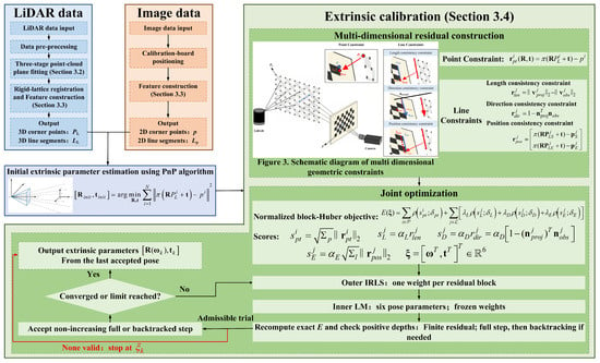
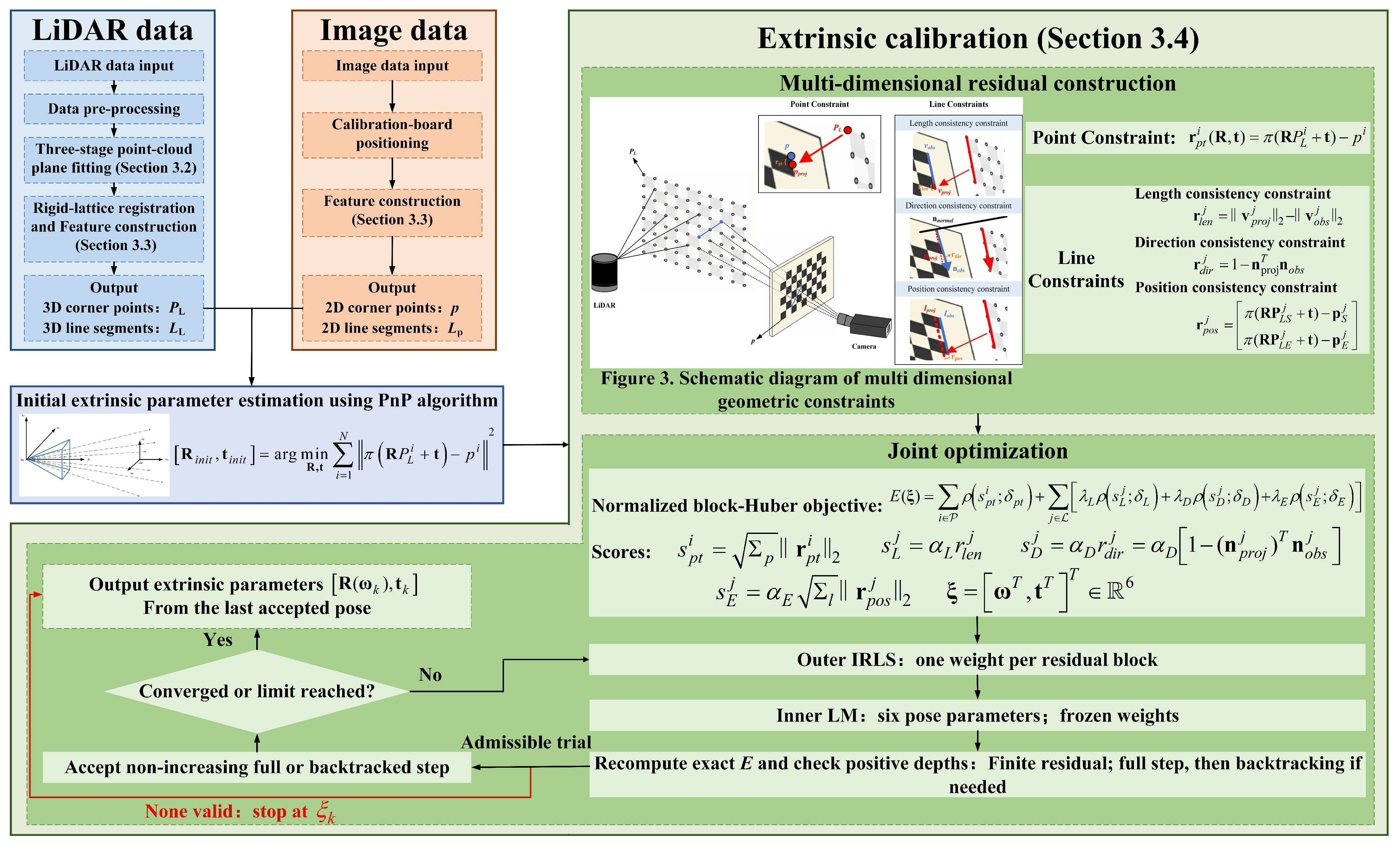
The overall framework is shown in Figure 2. The front end reconstructs the calibration-board plane from raw LiDAR points before extracting 3D point and line features. Given a raw point set ${\mathcal{P}}_{raw}={\{{\mathbf{P}}_i\in {\mathbb{R}}^3\}}_{i=1}^N$, RANSAC  [42] first estimates a coarse plane,

$$aX+bY+cZ+d=0,\mathbf{n}={[a,b,c]}^T.$$

(4)

Figure 2. Overall workflow of the proposed P3LPnP calibration framework. The front end uses random sample consensus (RANSAC), density-based spatial clustering of applications with noise (DBSCAN), and principal component analysis (PCA), followed by rigid-lattice registration. Perspective-n-point (PnP) initialization is followed by outer iteratively re-weighted least squares (IRLS) with an inner Levenberg–Marquardt (LM) solve. The pose is represented by a Rodrigues rotation vector and translation, and candidate steps are checked using the exact block-Huber objective.

Three non-collinear points are sampled in each iteration, and points whose perpendicular distance is less than ${\tau }_r=0.01$ m are retained as inliers. The threshold is chosen to be larger than small LiDAR ranging perturbations but smaller than the typical separation between the calibration board and background structures in the experiment. The same threshold is used for every scene and every front-end variant. The RANSAC stage suppresses large-scale background points but may still retain dense local clutter around the board.

The RANSAC candidates are refined by density-based spatial clustering of applications with noise (DBSCAN) [43] before PCA. Let $N_r$ denote the number of RANSAC candidates and let ${\overline{d}}_{10}$ be the mean, over all candidates, of the distances to the ten nearest other candidates; the zero self-distance is excluded. The DBSCAN parameters are

$$ϵ=c{\overline{d}}_{10},\mathrm{minPts}=\max \left(3,\min \left(20,\mathrm{round}\left(f{N}_r\right)\right)\right).$$

(5)

The default coefficients are $c=1.20$ and $f=0.05$. If at least one positive cluster is returned then the largest positive cluster is retained. If no positive cluster is returned then DBSCAN is repeated with $1.5ϵ$ and $\max (2,\mathrm{minPts}-1)$. If the repeated call also returns no positive cluster then all RANSAC candidates are retained; a result with fewer than three points is treated as a failure rather than omitted. PCA is then fitted to the retained set. This fallback rule is part of the implementation, although it was not activated in the matched sensitivity runs reported below.

Finally, PCA  [44] is applied to the refined board point set ${\mathcal{P}}_B$. Its centroid and covariance matrix are

$${\mathit{\mu }}_B={\displaystyle \frac{1}{M}}\sum _{\mathbf{P}\in {\mathcal{P}}_B}\mathbf{P},$$

(6)

$${\Sigma }_B={\displaystyle \frac{1}{M-1}}\sum _{\mathbf{P}\in {\mathcal{P}}_B}(\mathbf{P}-{\mathit{\mu }}_B){(\mathbf{P}-{\mathit{\mu }}_B)}^T,$$

(7)

where $M=\left|{\mathcal{P}}_B\right|$. The first two principal directions define the local board coordinate system, and the eigenvector associated with the smallest eigenvalue is used as the board normal. Table 1 summarizes the role of each front-end component.

Table 1. Functional analysis of the three-stage plane front end.

Front-End Variant	Operation Retained	Targeted Degradation	Expected Limitation If Used Alone	Role in This Work
Raw point cloud	None	None	Board plane may be corrupted by ground points, background clutter, and LiDAR ranging noise.	Baseline showing why direct fitting is unreliable.
RANSAC only	Global plane fitting	Large-scale outliers and background clutter	Dense local noise or nearby clutter may still be retained as inliers.	Provides a coarse but robust planar hypothesis.
RANSAC + DBSCAN	Global fitting + local cluster filtering	Residual dense outliers after RANSAC	Plane normal can still be affected by LiDAR ranging noise.	Extracts the dominant calibration-board cluster.
RANSAC + PCA	Global fitting + normal refinement	Outliers and Gaussian ranging noise	May retain local clutter if the RANSAC inlier set is mixed.	Refines the normal and builds a local board coordinate frame.
Ours	Global fitting + cluster purification + normal refinement	Outliers, local clutter, and ranging noise	Slightly higher complexity and parameter sensitivity.	Used as the final front end to obtain stable 3D point and line features.

Boldface identifies the complete front-end configuration used in the proposed method. RANSAC, random sample consensus; DBSCAN, density-based spatial clustering of applications with noise; PCA, principal component analysis.

3.3. Plane-Coordinate Lattice Registration and Feature Construction

After RANSAC and DBSCAN, let ${\mathbf{q}}_k\in {\mathbb{R}}^3$, $k=1,\dots ,N_B$, denote the retained board returns. PCA provides the centroid ${\mathit{\mu }}_B$, plane normal ${\mathbf{n}}_B$, and two orthonormal in-plane basis vectors ${\mathbf{b}}_1$ and ${\mathbf{b}}_2$. With $\mathbf{B}=\left[{\mathbf{b}}_1{\mathbf{b}}_2\right]$, the local planar coordinates are

$${\mathbf{u}}_k={\mathbf{B}}^T({\mathbf{q}}_k-{\mathit{\mu }}_B),\mathcal{U}={\left\{{\mathbf{u}}_k\right\}}_{k=1}^{N_B}.$$

(8)

PCA therefore estimates the supporting plane and a local coordinate basis; it does not by itself determine the in-plane grid origin, orientation, or corner ordering.

The target topology and physical pitches are treated as known design parameters. For a board with $R_B$ rows, $C_B$ columns, row pitch $s_y$, and column pitch $s_x$, the centered canonical lattice is

$${\mathbf{g}}_{rc}=\left[\begin{array}{c}\left(c-{\displaystyle \frac{C_B-1}{2}}\right)s_x\\ \left(r-{\displaystyle \frac{R_B-1}{2}}\right)s_y\end{array}\right],r=0,\dots ,R_B-1,c=0,\dots ,C_B-1.$$

(9)

Only a two-dimensional rigid transform is estimated, so the fitted target cannot shear or change scale. Defining ${\mathbf{v}}_{rc}(\theta ,\mathbf{t})={\mathbf{R}}_2\left(\theta \right){\mathbf{g}}_{rc}+\mathbf{t}$ and $d(\mathbf{x},\mathcal{S})={\min }_{\mathbf{s}\in \mathcal{S}}{\parallel \mathbf{x}-\mathbf{s}\parallel }_2$, the transform is obtained from the symmetric bidirectional truncated nearest-set objective

$$\begin{array}{cc}\hfill E(\theta ,\mathbf{t})=& {\displaystyle \frac{1}{R_B{C}_B}}\sum _{r,c}\min {\left(d\left({\mathbf{v}}_{rc},\mathcal{U}\right),{\tau }_g\right)}^2\hfill \\ \hfill & +{\displaystyle \frac{1}{N_B}}{\displaystyle \sum _{k=1}^{N_B}}\min {\left(d\left({\mathbf{u}}_k,{\mathcal{G}}_{\theta ,\mathbf{t}}\right),{\tau }_g\right)}^2,\hfill \end{array}$$

(10)

where ${\mathcal{G}}_{\theta ,\mathbf{t}}=\left\{{\mathbf{v}}_{rc}(\theta ,\mathbf{t})\right\}$. The truncation distance is set to ${\tau }_g=\max (s_x,s_y)$. Powell optimization is initialized with the two PCA-axis assignments, ${\theta }_0=0$ and ${\theta }_0=\pi /2$, and the solution with the lower objective is retained. The reconstructed three-dimensional nodes are

$${\widehat{\mathbf{P}}}_{rc}={\mathit{\mu }}_B+\mathbf{B}{\mathbf{v}}_{rc}(\widehat{\theta },\widehat{\mathbf{t}}).$$

(11)

In the synthetic reconstruction diagnostic, $R_B=6$, $C_B=9$, $s_x=0.04375$ m, and $s_y=0.05$ m, corresponding to target extents of $0.35\times 0.25$ m. These are target-geometry priors, not quantities inferred by PCA. The physical boundary is implied by the known target design rather than detected from coordinate extrema. The rigid-lattice fit uses no manually clicked 3D boundaries, per-scene manual input, or ground-truth coordinates. Ground truth is used only for the post-reconstruction synthetic error calculation.

The outer lattice vertices define four 3D contour segments,

$${\mathcal{L}}_L^j=({\mathbf{P}}_{LS}^j,{\mathbf{P}}_{LE}^j),j=1,\dots ,N_L,$$

(12)

and the corresponding image segments are represented as

$${\mathcal{L}}_p^j=({\mathbf{p}}_S^j,{\mathbf{p}}_E^j),{\mathbf{p}}_S^j,{\mathbf{p}}_E^j\in {\mathbb{R}}^2.$$

(13)

Geometric localization and correspondence ordering are treated separately. An unlabeled rectangular lattice is invariant to row and column reversals and to the transpose convention; therefore its 3D geometry alone does not define a unique ordered 2D–3D correspondence. The synthetic experiments used the known simulation topology to set this order. The real-data implementation instead loaded pre-associated $[v,u,X,Y,Z]$ records and used source-configured contour indices; it did not use the PCA lattice fit to infer real-data correspondences. Fully automatic ordering from raw measurements would require an additional cue, such as an asymmetric target marker, trackable return identities, or an independently validated coarse pose.

3.4. Multi-Dimensional Point-Line Optimization

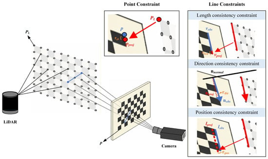
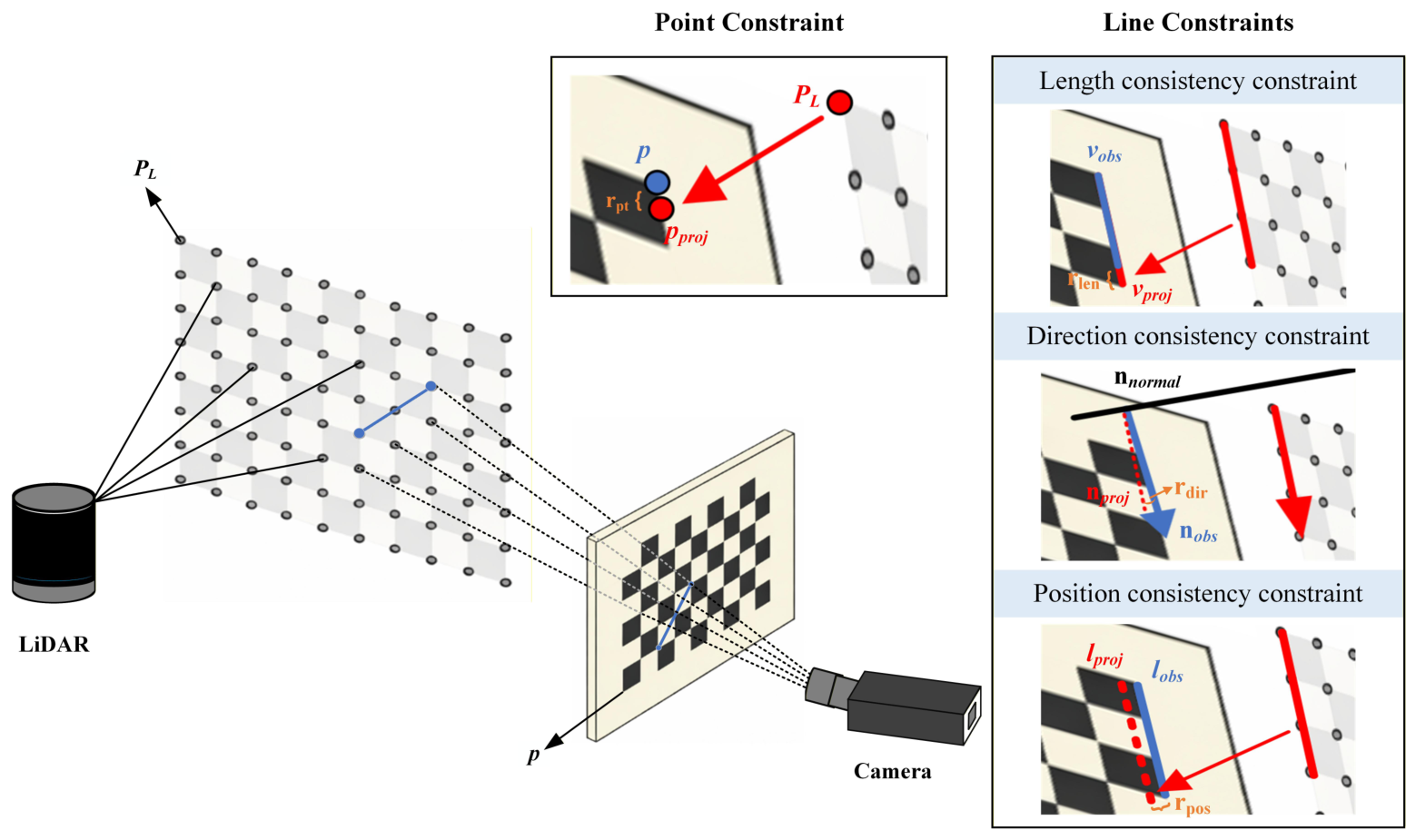
Relying on a single type of geometric constraint may not fully exploit the calibration-board geometry under sparse or noisy observations. Point constraints mainly provide local positional anchoring, whereas line constraints capture global structural information but are sensitive to line-extraction errors when used alone. Therefore, point re-projection and three complementary finite-line-segment constraints, including projected length, direction, and endpoint position, are jointly incorporated to improve cross-sensor geometric consistency and pose observability, as illustrated in Figure 3.

Figure 3. Schematic diagram of the multi-dimensional point-line geometric constraints used in P3LPnP.

The extrinsic parameters are initialized by a PnP estimate and then refined by nonlinear least squares. The initialization follows the point-only estimate shown in the workflow:

$$[{\mathbf{R}}_{init},{\mathbf{t}}_{init}]=\arg \underset{\mathbf{R},\mathbf{t}}{\min }{\displaystyle \sum _{i=1}^{N_p}}{∥\pi (\mathbf{R}{\mathbf{P}}_L^i+\mathbf{t})-{\mathbf{p}}^i∥}_2^2.$$

(14)

For a point correspondence $({\mathbf{P}}_L^i,{\mathbf{p}}^i)$, the point residual is

$${\mathbf{r}}_{pt}^i(\mathbf{R},\mathbf{t})=\pi (\mathbf{R}{\mathbf{P}}_L^i+\mathbf{t})-{\mathbf{p}}^i.$$

(15)

For the j-th 3D line segment and its observed image segment, the projected endpoints are

$${\mathbf{p}}_{S,proj}^j=\pi (\mathbf{R}{\mathbf{P}}_{LS}^j+\mathbf{t}),{\mathbf{p}}_{E,proj}^j=\pi (\mathbf{R}{\mathbf{P}}_{LE}^j+\mathbf{t}).$$

(16)

The projected and observed segment vectors are

$${\mathbf{v}}_{proj}^j={\mathbf{p}}_{E,proj}^j-{\mathbf{p}}_{S,proj}^j,{\mathbf{v}}_{obs}^j={\mathbf{p}}_E^j-{\mathbf{p}}_S^j.$$

(17)

The proposed line-segment model uses three complementary residuals. The length consistency residual is 

$$r_{len}^j={\parallel {\mathbf{v}}_{proj}^j\parallel }_2-{\parallel {\mathbf{v}}_{obs}^j\parallel }_2.$$

(18)

The direction consistency residual is

$$r_{dir}^j=1-{\left({\mathbf{n}}_{proj}^j\right)}^T{\mathbf{n}}_{obs}^j,{\mathbf{n}}_{proj}^j={\displaystyle \frac{{\mathbf{v}}_{proj}^j}{\parallel {\mathbf{v}}_{proj}^j{\parallel }_2}},{\mathbf{n}}_{obs}^j={\displaystyle \frac{{\mathbf{v}}_{obs}^j}{\parallel {\mathbf{v}}_{obs}^j{\parallel }_2}}.$$

(19)

The endpoint position residual is denoted as the position consistency residual in the workflow:

$${\mathbf{r}}_{pos}^j=\left[\begin{array}{c}\pi (\mathbf{R}{\mathbf{P}}_{LS}^j+\mathbf{t})-{\mathbf{p}}_S^j\\ \pi (\mathbf{R}{\mathbf{P}}_{LE}^j+\mathbf{t})-{\mathbf{p}}_E^j\end{array}\right].$$

(20)

For clarity, we use P, L, D, and E to denote the point-re-projection, projected-length, projected-direction, and endpoint-position terms, respectively. Thus, the $P+L+D$ variant does not contain the endpoint-position term, whereas Full P3LPnP is $P+L+D+E$. The endpoint residual for segment j is treated as one four-dimensional block containing the two projected endpoint differences.

Whether E supplies an additional observation depends on how its endpoints are obtained. In the main synthetic ablation, the line endpoints have the same nominal board-corner locations as boundary points, but their numerical observations are generated separately: the 3D line endpoints are defined by the ideal board contour and the 2D endpoints receive their own image perturbations. They therefore constitute an additional synthetic feature stream. In the shared-endpoint control, the endpoint term instead re-uses the exact perturbed 3D coordinates and 2D pixels already present in the point set; it then adds no observation and acts only as structured residual re-weighting.

Because the point, length, direction, and endpoint residuals have different scales, the robust kernel is applied to scalar block scores. Let ${\mathbf{r}}_{pt}^i\in {\mathbb{R}}^2$ be a point-re-projection residual, let $r_{\mathrm{len}}^j,r_{\mathrm{dir}}^j\in \mathbb{R}$ be the length and direction residuals, and let ${\mathbf{r}}_{\mathrm{pos}}^j\in {\mathbb{R}}^4$ be the stacked two-endpoint residual. The scores are

$$\begin{array}{cc}\hfill s_{pt}^i& =\sqrt{{\Sigma }_p}{\parallel {\mathbf{r}}_{pt}^i\parallel }_2,\hfill \\ \hfill s_L^j& ={\alpha }_L{r}_{len}^j,\hfill \\ \hfill s_D^j& ={\alpha }_D{r}_{dir}^j={\alpha }_D\left[1-{\left({\mathbf{n}}_{proj}^j\right)}^T{\mathbf{n}}_{obs}^j\right],\hfill \\ \hfill s_E^j& ={\alpha }_E\sqrt{{\Sigma }_l}{\parallel {\mathbf{r}}_{pos}^j\parallel }_2.\hfill \end{array}$$

(21)

Here, ${\Sigma }_p={\Sigma }_l=1$ are fixed scalar residual-scale factors, not covariance matrices. The normalization coefficients are ${\alpha }_L=5{\mathrm{px}}^{-1}$, ${\alpha }_D=6$, and ${\alpha }_E=0.5{\mathrm{px}}^{-1}$. The relative line-term weights are ${\lambda }_L={\lambda }_D={\lambda }_E=0.4$. The block-Huber objective used in the reported experiments is

$$\begin{array}{cc}\hfill E\left(\mathit{\xi }\right)=& \sum _{i\in \mathcal{P}}\rho (s_{pt}^i;{\delta }_{pt})\hfill \\ \hfill & +\sum _{j\in \mathcal{L}}\left[{\lambda }_L\rho (s_L^j;{\delta }_L)+{\lambda }_D\rho (s_D^j;{\delta }_D)+{\lambda }_E\rho (s_E^j;{\delta }_E)\right],\hfill \end{array}$$

(22)

where $\mathit{\xi }={[{\mathit{\omega }}^T,{\mathbf{t}}^T]}^T\in {\mathbb{R}}^6$ contains a Rodrigues rotation vector and translation. Each $\lambda$ is outside the corresponding robust kernel. The Huber function is applied to the score s, not to $s^2$:

$$\rho (s;\delta )=\left\{\begin{array}{cc}\frac{1}{2}{s}^2,\hfill & \left|s\right|\le \delta ,\hfill \\ \delta \left(\left|s\right|-\frac{1}{2}\delta \right),\hfill & \left|s\right|>\delta .\hfill \end{array}\right.$$

(23)

The thresholds are $({\delta }_{pt},{\delta }_L,{\delta }_D,{\delta }_E)=(3.0,2.5,15,2.0)$ in normalized score units.

The direction term requires a specific qualification. Since $r_{\mathrm{dir}}^j=1-{\left({\mathbf{n}}_{\mathrm{proj}}^j\right)}^T{\mathbf{n}}_{\mathrm{obs}}^j\in [0,2]$, the corresponding normalized score satisfies $s_D^j={\alpha }_D{r}_{\mathrm{dir}}^j\in [0,12]$ for ${\alpha }_D=6$. Consequently, the default threshold ${\delta }_D=15$ cannot be reached, and $W_D^{\left(k\right)}=1$ for every valid direction block. Under the reported configuration, the direction term therefore acts as a quadratic direction-consistency penalty rather than a robustly down-weighted term. Except for the Huber-threshold sensitivity tests in Section 5.3, the direction threshold is fixed at ${\delta }_D=15$; no robustness claim is made for this individual term.

The objective is minimized by outer iteratively re-weighted least squares (IRLS) and an inner Levenberg–Marquardt (LM) solve [45]. At accepted outer iterate ${\mathit{\xi }}_k$, the weight of each scalar block score is

$$W_b^{\left(k\right)}={\displaystyle \frac{\psi \left(s_b^{\left(k\right)}\right)}{s_b^{\left(k\right)}}}=\left\{\begin{array}{cc}1,\hfill & |s_b^{\left(k\right)}| \le {\delta }_b,\hfill \\ {\delta }_b/|s_b^{\left(k\right)}|,\hfill & |s_b^{\left(k\right)}| >{\delta }_b,\hfill \end{array}\right.$$

(24)

where $\psi =\partial \rho /\partial s$ and $W_b^{\left(k\right)}=1$ at zero. The multiplier applied to the residual components is $\sqrt{W_b^{\left(k\right)}}$, rather than $W_b^{\left(k\right)}$ itself. One common weight is applied to both components of a point block and one common weight to all four components of a line-endpoint block. The length and direction terms are scalar blocks. The line-block multipliers also include $\sqrt{{\lambda }_L}$, $\sqrt{{\lambda }_D}$, or $\sqrt{{\lambda }_E}$, respectively. Crucially, $W_b^{\left(k\right)}$ is computed once at the start of outer iteration k and remains fixed during every residual and Jacobian evaluation of the inner LM solve. The resulting quadratic surrogate, after adding a constant independent of $\mathit{\xi }$, has the same value and first derivative as the true Huber objective at ${\mathit{\xi }}_k$. The constant does not affect the inner minimizer and is therefore omitted from the least-squares residual vector. This fixed-weight surrogate is not treated as the true objective away from ${\mathit{\xi }}_k$. After the inner solve, the exact objective in Equation (22) is recomputed. A finite, positive-depth full step is accepted only when $E\left({\mathit{\xi }}_{k+1}\right)\le E\left({\mathit{\xi }}_k\right)+{10}^{-12}$. Otherwise, step fractions $1/2$, $1/4$, $1/8$, $1/16$, $1/32$, and $1/64$ are tested in that order against the same exact objective. If none is valid and non-increasing, the iteration terminates without accepting the candidate. Robust weights are updated only after an accepted outer iterate. The implementation permits at most 50 outer iterations and 220 inner function evaluations per outer iteration. The inner LM tolerances are ${10}^{-11}$ for the function, step, and gradient tests. The outer relative step and objective tolerances are ${10}^{-9}$. Non-finite residuals and non-positive projected depths are invalid. The pose is optimized using the six parameters $\mathit{\xi }={[{\mathit{\omega }}^T,{\mathbf{t}}^T]}^T$, where $\mathit{\omega }$ is a Rodrigues rotation vector. The rotation matrix is obtained from this vector, which preserves the $SO\left(3\right)$ constraint without an explicit matrix-projection step.

Table 2 clarifies the geometric role and limitation of each residual. In this paper, P3LPnP denotes the complete point-line formulation consisting of point re-projection plus the full finite-line-segment model.

Table 2. Geometric contribution of the finite line-segment constraints.

Constraint Setting	Residual Term Used	Main Geometric Information	Main Effect on Calibration	Limitation
Point only	Point re-projection	Local 3D–2D correspondence	Accurate when point observations are reliable and well distributed.	Sensitive when correspondences are sparse, poorly distributed, or inaccurate.
Line position only	Endpoint-position re-projection	Absolute image-plane position of line endpoints	Anchors line segments to the image and improves translation observability.	Sensitive to endpoint localization error.
Line length only	Projected segment length consistency	Scale and projected extent of line segment	Helps reduce scale-related ambiguity and supports translation estimation.	Weak when endpoints have similar depth or when line length is noisy.
Line direction only	Projected direction consistency	Orientation of projected line segment	Encodes orientation consistency; its isolated effect depends on the geometry and weighting.	Does not anchor endpoint location and poorly constrains translation.
Length + direction	Segment extent and orientation	Complementary structural line geometry	Couples projected extent and orientation without endpoint-position matching.	Still lacks the endpoint-position term E.
Full line segment	Length + direction + endpoint-position	Complete line-segment geometry	Uses line structure more completely than infinite-line models.	Can be affected by systematic line extraction bias.
Ours	Point + full line-segment constraints	Local point accuracy + global line structure	Balances point anchoring and line structural constraints under noisy or degraded observations.	Does not guarantee superiority when line features are severely corrupted.

Boldface identifies the complete point-line configuration used in P3LPnP.

Table 2 describes the geometric role of each residual and does not imply that every term produces an independently significant accuracy gain. The measured contributions are reported in the matched ablations in Section 5.

4. Experimental Protocol

4.1. Baseline Methods and Fairness

Seven methods were evaluated: graduated non-convexity PnP (GNCPnP) [28], a nonlinear supporting-line least-squares control denoted Line-LS, two-stage PnP (TSPnP) [17], OPnPL [25], P3LPnP, SQPnP [16], and depth-based efficient PnP (DEPnP) [29]. GNCPnP, TSPnP, and DEPnP were independently implemented from their published formulations. Line-LS minimizes the projected-endpoint-to-supporting-line incidence residual by nonlinear least squares from the common point-only initializer. It is an explicit control constructed for this study and is not presented as an implementation of the Mirzaei–Roumeliotis perspective-n-line (PnL) solver [33]. OPnPL denotes a numerical Python (version 3.13.9) port of the published ECCV 2016 companion implementation.

For every controlled comparison, all the methods received the same realization of each feature modality accepted by their formulation. The point-based methods used the common point correspondences, Line-LS used the common line correspondences, and OPnPL and P3LPnP used both. Thus, methods that consumed the same feature type were given identical observations, associations, and perturbations. No method was provided with method-specific feature re-extraction, noise realizations, or initialization selected according to its outcome. Because the compared formulations accepted different feature modalities, this shared-input rule does not imply that every method minimized an identical residual set.

The synthetic correspondences used the known simulation topology. The processed real-data files contained pre-associated $[v,u,X,Y,Z]$ records and source-configured contour indices. Consequently, the controlled solver comparisons evaluated pose estimation after feature association and did not independently validate the association process itself. Every planned run was retained, and no result cap, outcome-based seed selection, or method-specific perturbation was used.

4.2. Synthetic Data and Two-Regime Stress-Test Design

The synthetic scene contained a $6\times 9$ planar checkerboard, four boundary segments, and a pinhole camera with 

$$\mathbf{K}=\left[\begin{array}{ccc}800& 0& 640\\ 0& 800& 360\\ 0& 0& 1\end{array}\right].$$

The board was rotated by ${45}^{\circ }$ about the X-axis, and its pose relative to the camera was fixed across the experiments. The three-dimensional board coordinates received zero-mean Gaussian perturbations with a standard deviation of 3 mm.

The ground-truth LiDAR-to-camera pose used to generate the image observations was ${\mathit{\xi }}_{\mathrm{gt}}={[\pi /4,0,0,0.20,-0.03,1.20]}^T$, where the first three entries form the Rodrigues rotation vector in radians and the last three entries were the translation in meters.

The robustness evaluation contained one full-observation regime and one sparse-observation regime. The full-observation regime used all 54 checkerboard points. The per-coordinate Gaussian standard deviation of the image-point observations was varied from 0.5 to 5.0 pixels, while the line-endpoint noise remained fixed at 0.5 pixels and no deterministic line bias was applied. This test evaluated whether finite line-segment information can compensate for progressively degraded point localization when the complete point set remains available.

The sparse-observation regime used 12 checkerboard points selected once by deterministic farthest-point sampling in the board $XY$ coordinates, starting from the first grid point. The selection depended only on the known board geometry and used neither image measurements nor method outcomes. Two complementary perturbation tests were performed in this regime. In the joint-noise test, the same per-coordinate Gaussian standard deviation was applied to the 12 point observations and all the line endpoints, and it was varied from 0.5 to 3.5 pixels. In the coherent-bias test, random point and line noise was fixed at 0.5 pixels, while a common bias magnitude was varied from 0 to 2.5 pixels. The point observations were displaced radially from the projected board center, and the contour segments were displaced along their outward normals. These tests respectively represented joint random degradation and a shared systematic feature-localization bias under sparse point support.

The two regimes used the same camera, board geometry, board pose, four finite segments, seven method implementations, P3LPnP parameters, validity rules, evaluation metrics, and 30 pre-declared random seeds (11,001–11,030). Every planned run was retained, with no outcome-based seed selection, result clipping, or per-level parameter adjustment. The difference in point count was intentional: the full-observation regime tested the benefit of line information when dense point support is available, whereas the sparse-observation regime evaluated robustness when point support is deliberately limited. Method rankings and degradation trends were therefore interpreted within each protocol; absolute ordinate values were not compared directly between the two regimes.

For each estimated pose, the clean-reference re-projection error was the mean Euclidean image distance evaluated against the noise-free point projections. The noisy-point fit error was evaluated against the perturbed image points supplied to the optimizer. The translation error was the Euclidean distance between the estimated and ground-truth translations and is reported in millimeters. The rotation error was the geodesic angular distance between the estimated and ground-truth rotations and is reported in degrees. Both mean and median pose errors are reported to distinguish typical performance from sensitivity to occasional large errors. All cross-method comparisons were paired by random seed.

4.3. Real Records and Controlled Sparse-to-Dense Replay

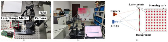
The physical system consisted of a 639 nm laser range meter with scanning controlled by a fast steering mirror (FSM) and a rigidly mounted $1280\times 720$ visible-light camera. The available dataset contained processed correspondence records with 100, 2500, and 10,000 points from the same system, scene, acquisition session, and processing chain. The records store rectified image coordinates and LiDAR coordinates. All image observations were rectified before optimization, and the projection model did not apply lens distortion a second time. Accordingly, the optimization used a zero residual-distortion vector. For the real-record experiments, the rectified intrinsic matrix was

$${\mathbf{K}}_{\mathrm{real}}=\left[\begin{array}{ccc}908.472066& 0& 657.090439\\ 0& 908.472066& 383.271336\\ 0& 0& 1\end{array}\right].$$

(25)

The synthetic experiments used the intrinsic matrix specified in Section 4.2.

The 100-point record was an exact subset of the 10,000-point record. These 100 correspondences were used as the sparse calibration input and were removed from the larger record, leaving 9900 same-session correspondences for held-out evaluation without re-optimization. The 2500-point record was reserved solely for qualitative projection and textured reconstruction and was excluded from all quantitative cross-method comparisons.

A deterministic replay of unchanged correspondences would not have provided run-to-run variability. Therefore, only the sparse calibration inputs were perturbed in 30 paired runs using the pre-declared seeds 11,001–11,030. The three-dimensional points received zero-mean Gaussian noise with a standard deviation of 3 mm, the image points received per-coordinate Gaussian noise with a standard deviation of 1.5 pixels, and the line endpoints received per-coordinate Gaussian noise with a standard deviation of 0.5 pixels. The corresponding unperturbed 100-point observations and the unperturbed 9900-point held-out set were used as evaluation references.

Four line segments were formed from the perimeter of the $10\times 10$ sparse scan grid. These segments constituted a reproducible scan-grid perimeter surrogate rather than an independently measured physical checkerboard boundary. The experiment was therefore interpreted as a real-record-based controlled perturbation test and a same-session sparse-to-dense consistency check. Because all the records originated from one sensor system, one mounting configuration, one scene, and one processing chain, the protocol is not presented as an independent multi-system accuracy or generalizability benchmark.

5. Results

5.1. Front-End Reconstruction Ablation

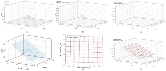
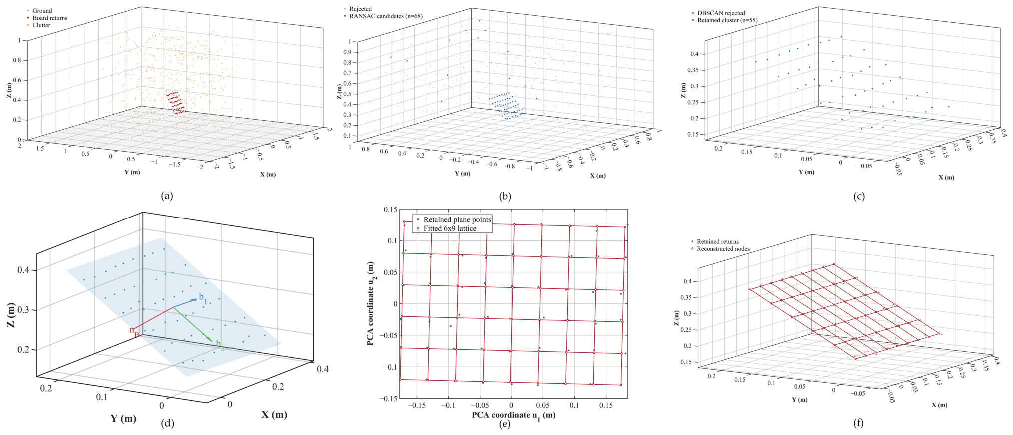
Figure 4 illustrates the plane-guided front-end reconstruction using seed 7001, the first entry in the fixed 30-scene list; the example was not selected according to its reconstruction error. Panel (a) uses the simulator component labels only to visualize the composition of the input scene. A fixed $z>0.05$ m gate removed the simulated ground layer before the three-stage procedure. RANSAC then produced 68 plane candidates, and the default DBSCAN setting ($ϵ=0.194668$ m and $\mathrm{minPts}=3$ for this scene) retained 55 points without invoking the fallback. PCA estimated the supporting plane and its local basis, after which the known-size rigid lattice described in Section 3.3 was registered in the plane and back-projected into 3D. Neither the synthetic ground-truth coordinates nor manual boundary selections entered the fit.

Figure 4. Plane-guided front-end reconstruction for the first pre-declared synthetic scene (seed 7001): (a) Raw simulated scene. (b) RANSAC plane candidates after the fixed simulation-only ground-removal gate. (c) Dominant local cluster retained by DBSCAN. (d) PCA plane and local orthonormal basis. (e) Registration of the known-size $6\times 9$ rigid lattice in PCA-plane coordinates. (f) Reconstructed lattice back-projected into 3D.

For this fixed visualization scene, the rigid-lattice registration reconstructed 54 unique nodes and gave a permutation-invariant corner root mean square error (RMSE) of 0.695 mm. This single-scene value is descriptive only. The 30-scene comparison is reported below, and its corner-localization RMSE is distinct from the point-to-plane RMSE in Table 3.

Table 3. Matched front-end ablation (mean ± sample standard deviation over 30 fixed scenes).

Variant	Normal Error (deg)	Plane RMSE (mm)
Raw PCA	$45.646\pm 1.862$	$219.145\pm 12.983$
RANSAC model	$1.118\pm 0.594$	$2.264\pm 0.979$
RANSAC + PCA	$0.971\pm 0.573$	$1.697\pm 0.983$
RANSAC + DBSCAN + PCA	0.342 ± 0.183	0.673 ± 0.320

Boldface highlights the results of the complete RANSAC–DBSCAN–PCA front end. RMSE, root mean square error.

Table 3 reports a matched front-end ablation over 30 fixed synthetic scenes (seeds 7001–7030). Each scene contained 54 board returns with independent 3 mm coordinate noise, a ground plane, and 500 random clutter points. A synthetic-only $z>0.05$ m gate removed the known ground plane without using board labels. RANSAC then used a 0.01 m distance threshold and 5000 trials. Normal error was the angle to the true board normal, and plane RMSE was the root mean square orthogonal distance from the noise-free board nodes to the estimated plane. Ground truth was used only for evaluation.

Compared with raw PCA, the complete front end reduced the mean plane RMSE from 219.145 to 0.673 mm and the mean normal error from $45.{646}^{\circ }$ to $0.{342}^{\circ }$. The intermediate variants indicate that RANSAC removed most of the gross background contamination, while DBSCAN purification and final PCA refinement provided the additional improvement required for accurate plane recovery.

The geometry-constrained rigid-lattice registration was compared with an extrema-and-snapping baseline using the same retained board clusters from 30 fixed synthetic scenes. The baseline formed a grid over the coordinate-wise PCA extrema and independently snapped each provisional node to its nearest retained return. It produced duplicate nodes in 16 of the 30 runs and a permutation-invariant corner RMSE of $37.865\pm 40.910$ mm. The rigid-lattice registration produced 54 unique co-planar nodes in every run and a corner RMSE of $1.001\pm 0.371$ mm. Its corner RMSE was lower in all 30 paired scenes; the mean paired difference, defined as rigid-lattice registration minus the baseline, was $-36.864$ mm, with a 95% confidence interval of $[-52.047,-21.681]$ mm. Truncation distances of 0.04, 0.05, and 0.08 m gave mean RMSEs of 0.964, 1.001, and 1.004 mm, respectively. Hungarian one-to-one matching and ground truth were used only for this post-fit, permutation-invariant evaluation.

5.2. Line-Constraint Ablation

The matched line-term ablation used 30 fixed random seeds (8101–8130). Each run contained the same 54 point correspondences for every variant, with a per-coordinate 3D perturbation of 3 mm and 1.5-pixel image noise. The four contour segments were constructed as follows: their 3D endpoints were defined by the ideal board boundary, and their image endpoints were generated independently with 0.5-pixel noise; the first endpoint of the first segment additionally received a fixed $(0.5,0.5)$-pixel perturbation. All the variants used the same point-only initialization, residual scales, and outer IRLS procedure with weights fixed during each inner LM solve. The ground-truth pose was used only for evaluation. All 30 planned runs were retained, and paired differences were accompanied by two-sided 95% Student-t confidence intervals.

The noisy-point fit was the mean Euclidean re-projection error against the noisy point pixels used by the optimizer. The clean-reference re-projection compared the estimated projection of the same perturbed 3D points with their noise-free image projections generated by the ground-truth pose; it was used only for evaluation and was not an additional observation.

Table 4 separates two questions. Panel (a) measured the conditional benefit of independently generated synthetic line observations. Panel (b) tested the residual-re-weighting explanation by making the line endpoints exactly identical to existing boundary-point observations. In panel (b), $P+B_{\mathrm{sep}}$ repeated each endpoint as a separate 2D Huber block, whereas $P+E_{\mathrm{shared}}$ grouped the same two endpoints into the 4D block used by the endpoint-position term. The controls had identical endpoint multiplicity, normalization, relative weight, and Huber threshold; only the robust-block grouping differed.

Table 4. Matched synthetic line-term ablation and shared-endpoint control (mean ± sample standard deviation over 30 fixed seeds).

Variant	Active Terms	Noisy-Point Fit (px)	Clean Reference (px)	Trans. (mm)	Rot. (deg)
(a) Independently generated synthetic line observations
Point only	P	$1.862\pm 0.139$	$0.441\pm 0.126$	$5.094\pm 3.144$	$0.341\pm 0.149$
Point + length	$P+L$	$1.874\pm 0.144$	$0.407\pm 0.118$	$3.459\pm 2.109$	$0.325\pm 0.146$
Point + direction	$P+D$	$1.862\pm 0.139$	$0.441\pm 0.126$	$5.094\pm 3.144$	$0.341\pm 0.149$
Point + endpoint position	$P+E$	$1.862\pm 0.139$	$0.429\pm 0.123$	$4.901\pm 3.063$	$0.330\pm 0.145$
Point + length + direction (no E)	$P+L+D$	$1.874\pm 0.144$	$0.407\pm 0.118$	$3.459\pm 2.109$	$0.325\pm 0.146$
Full P3LPnP	$P+L+D+E$	$1.875\pm 0.144$	$0.399\pm 0.116$	$3.424\pm 2.089$	$0.317\pm 0.142$
(b) Exact re-use of existing boundary-point observations
Point only	P	$1.862\pm 0.139$	$0.441\pm 0.126$	$5.094\pm 3.144$	$0.341\pm 0.149$
Repeated boundary points	$P+B_{\mathrm{sep}}$	$1.862\pm 0.139$	$0.443\pm 0.121$	$5.061\pm 3.017$	$0.341\pm 0.150$
Joint shared-endpoint block	$P+E_{\mathrm{shared}}$	$1.862\pm 0.139$	$0.443\pm 0.122$	$5.056\pm 3.018$	$0.340\pm 0.150$

Lower values are better. In panel (a), E uses independently generated line observations at the same nominal boundary locations. In panel (b), both added conditions re-use the exact perturbed 3D and 2D boundary-point records from P and hence contain no new observation. Clean reference is an evaluation-only metric and is not optimized. Trans., translation; Rot., rotation; px, pixels.

With independently generated line observations, Full P3LPnP reduced the clean-reference re-projection error from $0.441\pm 0.126$ to $0.399\pm 0.116$ pixels and the translation error from $5.094\pm 3.144$ to $3.424\pm 2.089$ mm relative to Point only. The paired Full-minus-Point differences were $-0.04178$ pixels (95% CI $[-0.06948,-0.01408]$) and $-1.67046$ mm (95% CI $[-2.61490,-0.72602]$), respectively. The observed rotation difference was $-0.{02418}^{\circ }$, but its 95% CI ${[-0.06728,0.01892]}^{\circ }$ included zero. Conversely, the noisy-point fit increased by 0.01273 pixels (95% CI $[0.00726,0.01820]$), revealing a small trade-off between fitting the noisy point pixels and incorporating the separately generated line observations.

The length term accounted for most of the improvement under this protocol. Adding the direction score alone changed all four reported means by less than ${10}^{-5}$, so it is not interpreted as a strong independent contributor. The endpoint-position term had a smaller but measurable incremental effect: Full minus $P+L+D$ reduced clean-reference re-projection by 0.00822 pixels (95% CI $[-0.00962,-0.00681]$), translation by 0.03517 mm (95% CI $[-0.04673,-0.02361]$), and rotation by $0.{00811}^{\circ }$ (95% CI ${[-0.01028,-0.00595]}^{\circ }$). This comparison is valid because $P+L+D$ explicitly excludes E.

When the endpoint block exactly re-used existing boundary-point observations, joint 4D grouping and matched separable re-weighting differed by only $-0.00035$ pixels in clean reference re-projection, $-0.00499$ mm in translation, and $-0.{00021}^{\circ }$ in rotation. All corresponding 95% confidence intervals included zero. A shared-endpoint term was therefore interpreted as structured re-weighting, not as an independent geometric observation. The main panel demonstrates only a conditional synthetic benefit when line features were generated separately and more accurately than the point stream; it does not establish that endpoints in a real sensor record are independent.

5.3. Matched Local Parameter Sensitivity

Table 5 reports two matched local sensitivity studies, with front-end reconstruction and back-end calibration evaluated separately. Each study varied one parameter group while keeping the corresponding observations and evaluation protocol fixed. Panel (a) changes only the DBSCAN parameter pair $(c,f)$ on the same 30 scenes and RANSAC candidate sets used in Table 3. Its default row reproduces the complete RANSAC + DBSCAN + PCA configuration reported in Table 3; the scene and RANSAC-candidate hashes agreed for every seed. Panel (b) is a separate back-end study that re-used the 30 fixed observations and point-only initializations of Table 4. It changed either all three outer line-cost multipliers or all four Huber thresholds while leaving the scene, features, residual normalization, direction formula, and solver unchanged.

Table 5. Matched local parameter sensitivity of the front end and back end (mean ± sample standard deviation; 30 fixed seeds per setting).

(a) Front-End DBSCAN Sensitivity
Setting	c	f	Normal error (deg)	Plane RMSE (mm)
Lower-scale	0.96	0.03	$0.303\pm 0.136$	$0.610\pm 0.261$
Default	1.20	0.05	$0.342\pm 0.183$	$0.673\pm 0.320$
Higher-scale	1.80	0.08	$0.421\pm 0.266$	$0.815\pm 0.424$
(b) Back-End Weight and Huber-Threshold Sensitivity
Setting	Noisy-point fit (px)	Clean reference (px)	Trans. (mm)	Rot. (deg)
Default	$1.875\pm 0.144$	$0.399\pm 0.116$	$3.424\pm 2.089$	$0.317\pm 0.142$
Line weights $0.5\times$	$1.869\pm 0.142$	$0.399\pm 0.120$	$3.532\pm 2.329$	$0.307\pm 0.140$
Line weights $1.5\times$	$1.878\pm 0.145$	$0.400\pm 0.116$	$3.407\pm 2.079$	$0.324\pm 0.149$
Huber thresholds $0.67\times$	$1.869\pm 0.142$	$0.410\pm 0.119$	$3.579\pm 2.216$	$0.321\pm 0.145$
Huber thresholds $1.5\times$	$1.879\pm 0.145$	$0.394\pm 0.118$	$3.289\pm 2.014$	$0.313\pm 0.150$

Panel (a) used seeds 7001–7030. Here $ϵ=c{\overline{d}}_{10}$ and $\mathrm{minPts}=\max (3,\min (20,\mathrm{round}\left(f{N}_r\right)))$; all 90 planned runs were retained. Panel (b) used the separate seeds 8101–8130. The default line multipliers were $({\lambda }_L,{\lambda }_D,{\lambda }_E)=(0.4,0.4,0.4)$ and the default Huber thresholds were $({\delta }_{pt},{\delta }_L,{\delta }_D,{\delta }_E)=(3.0,2.5,15.0,2.0)$. The noisy-point fit was measured against the pixel observations used by the optimizer. The clean reference was evaluated against the noise-free image projection of the same perturbed 3D points and was not optimized. All 150 planned back-end runs were retained. The two panels used different, explicitly matched experimental units and were not pooled.

For panel (a), the actual $ϵ$ ranges were 0.1086–0.1566 m, 0.1357–0.1957 m, and 0.2036–0.2936 m for the lower-scale, default, and higher-scale settings; the corresponding minPts values were 3, 3, and 5 in all 30 scenes. Neither fallback was triggered. Relative to default, the paired mean plane-RMSE differences were $-0.0628$ mm (95% CI $[-0.1224,-0.0032]$) and $+0.1419$ mm (95% CI $[0.0331,0.2506]$). These paired results indicate small but statistically detectable local sensitivity to the tested DBSCAN parameter scales.

For panel (b), all 150 optimizations converged and every accepted outer step had a non-increasing true Huber objective. Across the four perturbations, the mean clean-reference error ranged from 0.394 to 0.410 pixels, translation error from 3.289 to 3.579 mm, and rotation error from $0.{307}^{\circ }$ to $0.{324}^{\circ }$. For these three evaluation quantities, every paired 95% confidence interval relative to default contained zero. These results support local stability around the reported scales; they do not establish global optimality or invariance. The direction score did not cross its Huber threshold in any of the five back-end settings.

5.4. Synthetic Calibration Results

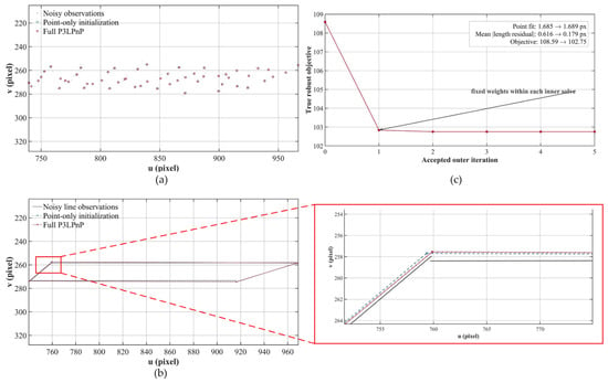
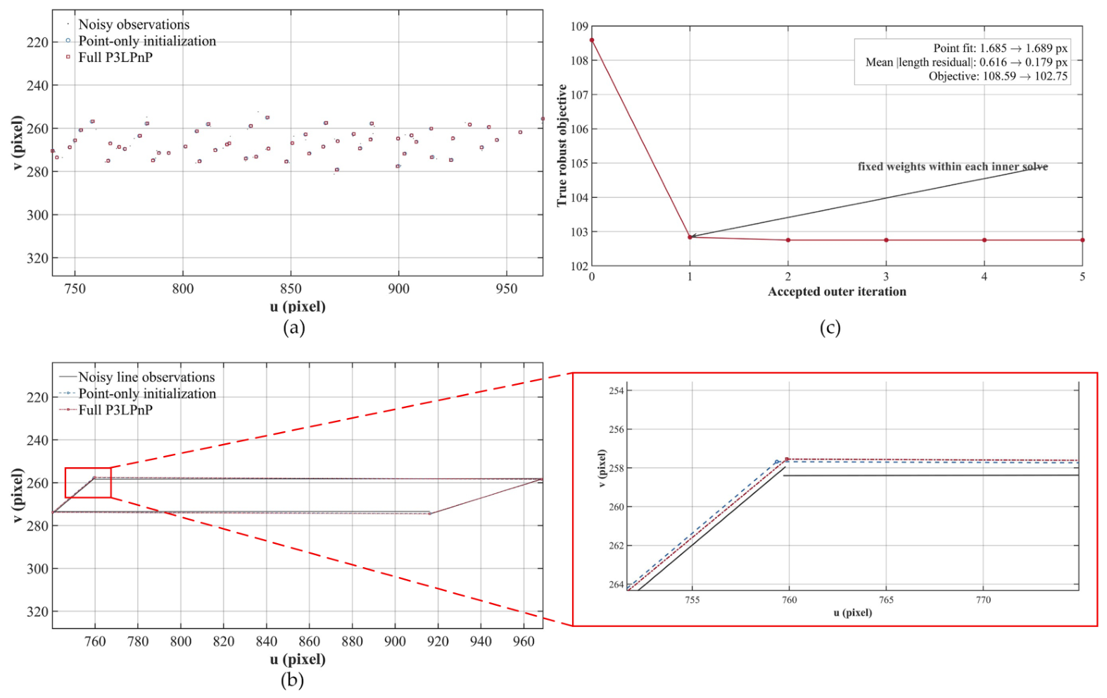
Figure 5 separately illustrates the back-end refinement using seed 8101, the first entry in the fixed Table 4 seed list. It was not the same simulated scene as Figure 4 and is not presented as a serial continuation of that front-end example. The point-only initialization was obtained from noisy 3D–2D point correspondences without using the true pose or line observations. The full P3LPnP model was then optimized using the independent-line protocol adopted for the main line-constraint ablation. Because the line projections are difficult to distinguish at the scale of the complete board, the red boxed region in Figure 5b is additionally shown in an enlarged view.

Figure 5. Fixed-seed illustration of point-line refinement using seed 8101: (a) Noisy point observations and the projections obtained from the point-only initialization and the full P3LPnP estimate. (b) Independently perturbed finite-line observations and the projected segments obtained from the point-only initialization and full P3LPnP estimate. The enlarged view at the lower right corresponds to the red boxed region in panel (b) and shows the otherwise difficult-to-observe differences among the three line-segment results. (c) Exact block-Huber objective at initialization and after each accepted IRLS outer iteration.

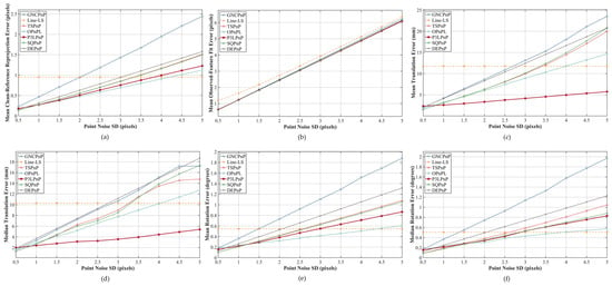
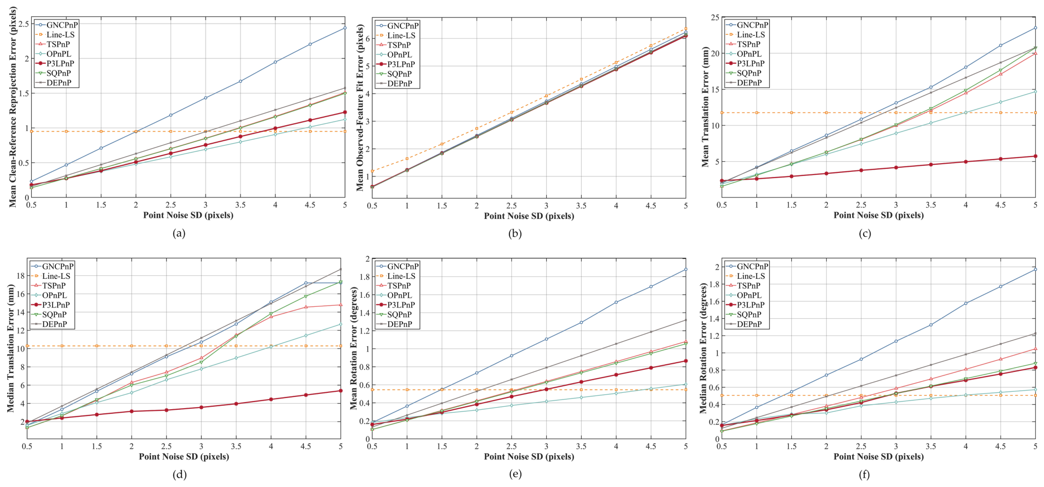
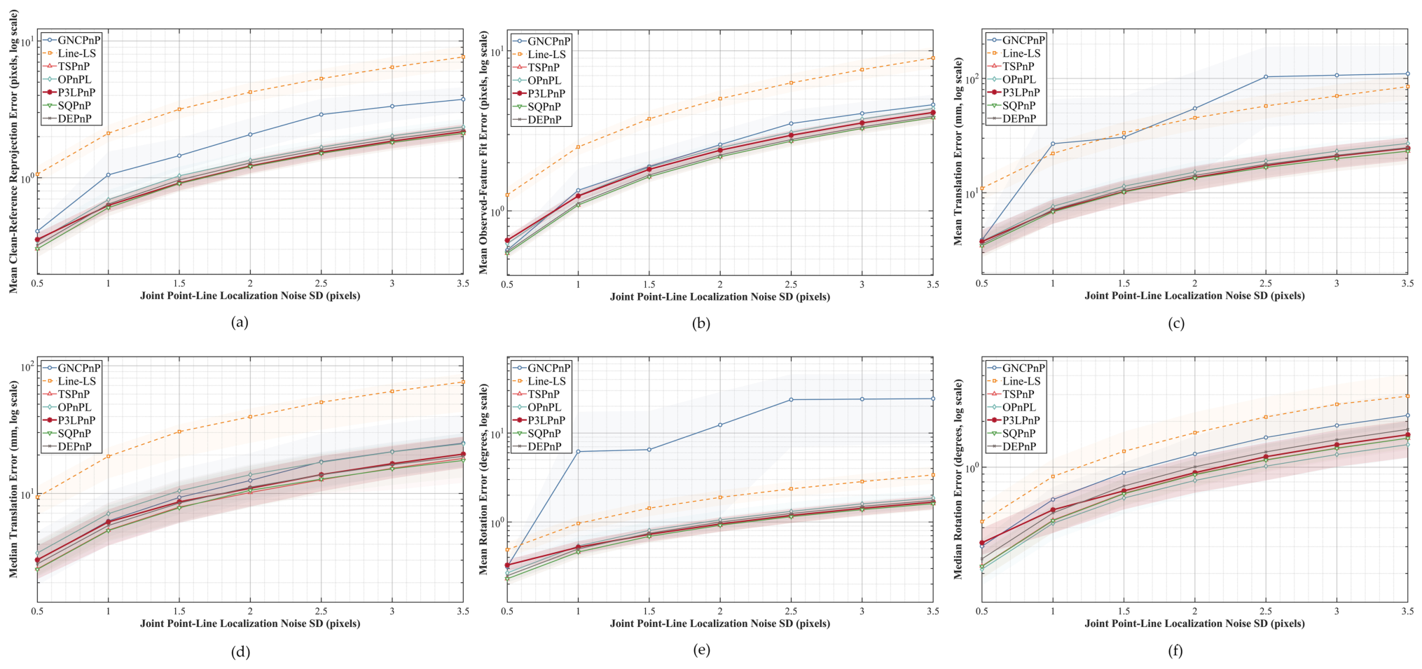
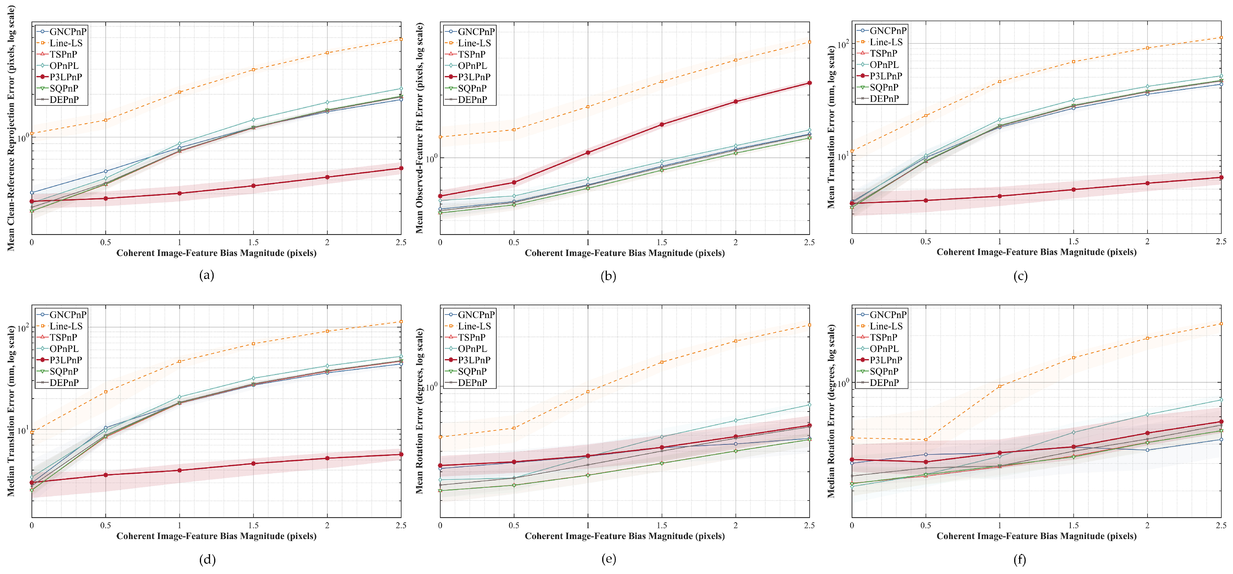
Figure 6, Figure 7 and Figure 8 jointly evaluated robustness under three complementary perturbation conditions following the two-regime design in Section 4.2: Gaussian image-point noise in the full-observation regime (Figure 6), joint point-and-line localization noise in the sparse-observation regime (Figure 7), and coherent image-feature bias in the sparse-observation regime (Figure 8). In each figure, panel (a) reports clean-reference re-projection error, panel (b) reports fit to the perturbed point observations, and the remaining panels report translation and rotation errors relative to the known synthetic pose.

Figure 6. Sensitivity to Gaussian image-point noise in the full-observation setting: (a) Mean clean-reference re-projection error. (b) Mean fit error to the noisy point observations. (c) Mean translation error. (d) Median translation error. (e) Mean rotation error. (f) Median rotation error. Each curve reports the mean or median over 30 retained runs.

Figure 7. Sensitivity to joint point-and-line localization noise in the sparse-observation setting: (a) Mean clean-reference re-projection error. (b) Mean fit error to the noisy point observations. (c) Mean translation error. (d) Median translation error. (e) Mean rotation error. (f) Median rotation error. All ordinates use logarithmic scales. Curves report means or medians over 30 retained runs, and shaded bands denote pointwise 95% bootstrap confidence intervals. The horizontal axis gives the per-coordinate noise standard deviation (SD) in pixels. Band colors correspond to the method curves, and overlapping confidence bands are displayed by superimposing their colors.

Figure 8. Sensitivity to coherent image-feature bias in the sparse-observation setting: (a) Mean clean-reference re-projection error. (b) Mean fit error to the noisy point observations. (c) Mean translation error. (d) Median translation error. (e) Mean rotation error. (f) Median rotation error. All ordinates use logarithmic scales. Curves report means or medians over 30 retained runs, and shaded bands denote pointwise 95% bootstrap confidence intervals. Band colors correspond to the method curves, and overlapping confidence bands are displayed by superimposing their colors.

In the fixed-seed illustration in Figure 5, five accepted outer iterations reduced the exact block-Huber objective from 108.591 to 102.754. The mean absolute projected-length residual decreased from 0.616 to 0.179 pixels, whereas the noisy-point fit changed slightly from 1.685 to 1.689 pixels. Figure 5 therefore illustrates finite-segment refinement and monotone objective acceptance rather than stand-alone comparative accuracy. Aggregate line-constraint effects are reported over 30 fixed seeds in Table 4, and cross-method robustness is evaluated in Figure 6, Figure 7 and Figure 8. Under the 50-iteration limit, all 60 full-model runs converged, and every accepted outer step produced a non-increasing exact objective. Scalar Huber tests and finite-difference gradient checks further confirmed implementation consistency, but do not imply global optimality.

Under increasing point noise, P3LPnP showed its clearest advantage in translation, achieving the lowest mean and median translation errors at nine of the ten tested levels (1.0–5.0 pixels). At 5.0 pixels, its mean translation error was 5.739 mm, with a paired difference of $-8.942$ mm relative to OPnPL (95% bootstrap CI: $[-12.681,-5.779]$ mm). However, P3LPnP ranked third in mean clean-reference re-projection and rotation error at this level, indicating a metric-specific rather than uniform advantage. Figure 6 therefore demonstrates improved translation stability when point localization deteriorated while line observations remained relatively reliable. Line-LS is constant in panels (a) and (c)–(f) because it used only the fixed line observations, whereas panel (b) varies because the evaluated point observations were perturbed.

When point and line localization were jointly degraded in the sparse-observation regime (Figure 7), neither feature modality remained clean. All seven methods degraded as the common localization noise increased. At 3.5 pixels, P3LPnP ranked third in mean clean-reference re-projection, translation, and rotation error, with values of 2.176 pixels, 24.556 mm, and $1.{673}^{\circ }$, respectively. These errors were 7.59%, 8.97%, and 9.94% lower than those of OPnPL, but the paired 95% confidence intervals included zero. Thus, P3LPnP remained competitive under sparse joint random degradation, without demonstrating statistically significant superiority.

Systematic feature bias was evaluated separately from zero-mean random noise, as shown in Figure 8. From 0.5 to 2.5 pixels of bias, P3LPnP ranked first at every tested level in mean clean-reference re-projection, mean translation, and median translation error. At 2.5 pixels, these values were 0.605 pixels, 6.370 mm, and 5.692 mm, respectively; the next-lowest values were 1.836 pixels, 43.256 mm, and 43.655 mm. P3LPnP did not rank first in rotation error and was fifth at the largest bias. Its comparatively large observation-fit value in panel (b), together with its low clean-reference and translation errors, indicates that the solution does not simply follow the imposed biased measurements.

Taken together, the full-observation point-noise benchmark shows how line information can stabilize translation when point localization deteriorates. The sparse joint-noise test showed competitive, but not uniformly best, performance when both feature types became noisy. The sparse coherent-bias test identified the condition under which the combined constraints provided the strongest benefit. No conclusion relied on comparing absolute error magnitudes between the 54-point and 12-point regimes.

5.5. Real-Record-Based Validation

The physical calibration setup is shown in Figure 9. As defined in Section 4, the quantitative experiment was a 30-run controlled perturbation replay on processed real-record geometry. No optimization was performed on the unperturbed 9900-point held-out set.

Figure 9. Real LiDAR–camera calibration experiment: (a) LiDAR–camera system with a fast steering mirror (FSM). (b) Calibration experiment. (c) Schematic diagram of the calibration setup.

As shown in Table 6, all seven methods returned valid poses in all 30 runs. P3LPnP gave the lowest observed mean horizontal, vertical, and Euclidean errors. Its mean Euclidean error was 0.356 pixels, compared with 0.376 pixels for OPnPL. The pose estimated from each perturbed 100-point input was transferred to the 9900 held-out correspondences without re-optimization. As shown in Table 7, P3LPnP again gave the lowest observed mean horizontal, vertical, and Euclidean errors. The mean Euclidean errors of P3LPnP and OPnPL were 0.338 and 0.359 pixels, respectively. In the paired analysis, the P3LPnP–OPnPL mean differences were $-0.0205$ pixels on the sparse reference (95% bootstrap confidence interval $[-0.0435,0.0026]$) and $-0.0208$ pixels on the held-out set ($[-0.0423,0.0006]$). Because both intervals included zero, the paired analysis did not establish a statistically significant difference between P3LPnP and OPnPL under this protocol. P3LPnP had the lowest observed mean errors, but a statistically significant advantage over OPnPL was not demonstrated.

Table 6. Clean-reference re-projection errors on the 100-point sparse record under controlled perturbation of the calibration inputs. Values are the mean ± standard deviation across 30 paired runs.

Algorithm	Valid Runs	Mean $\left|\mathit{u}\right|$ (px)	Mean $\left|\mathit{v}\right|$ (px)	Mean $\sqrt{{\mathit{u}}^2+{\mathit{v}}^2}$ (px)
GNCPnP	30	$0.473\pm 0.190$	$0.393\pm 0.188$	$0.691\pm 0.209$
Line-LS	30	$0.404\pm 0.189$	$0.237\pm 0.125$	$0.509\pm 0.206$
TSPnP	30	$0.316\pm 0.134$	$0.236\pm 0.102$	$0.436\pm 0.138$
OPnPL	30	$0.269\pm 0.118$	$0.209\pm 0.080$	$0.376\pm 0.117$
P3LPnP	30	0.250 ± 0.113	0.202 ± 0.085	0.356 ± 0.118
SQPnP	30	$0.304\pm 0.118$	$0.229\pm 0.082$	$0.421\pm 0.115$
DEPnP	30	$0.513\pm 0.295$	$0.301\pm 0.143$	$0.643\pm 0.336$

Boldface identifies the proposed P3LPnP method and its results. The unit px denotes pixels.

Table 7. Re-projection errors on the 9900 same-session held-out correspondences. The pose was estimated from the perturbed 100-point input and was transferred without re-optimization. Values are the mean ± standard deviation across 30 paired runs.

Algorithm	Valid Runs	Mean $\left|\mathit{u}\right|$ (px)	Mean $\left|\mathit{v}\right|$ (px)	Mean $\sqrt{{\mathit{u}}^2+{\mathit{v}}^2}$ (px)
GNCPnP	30	$0.444\pm 0.200$	$0.375\pm 0.195$	$0.655\pm 0.220$
Line-LS	30	$0.411\pm 0.205$	$0.227\pm 0.126$	$0.507\pm 0.216$
TSPnP	30	$0.296\pm 0.136$	$0.224\pm 0.103$	$0.411\pm 0.136$
OPnPL	30	$0.257\pm 0.120$	$0.199\pm 0.079$	$0.359\pm 0.115$
P3LPnP	30	0.237 ± 0.115	0.194 ± 0.084	0.338 ± 0.117
SQPnP	30	$0.285\pm 0.120$	$0.216\pm 0.081$	$0.395\pm 0.112$
DEPnP	30	$0.469\pm 0.266$	$0.276\pm 0.129$	$0.589\pm 0.299$

Boldface identifies the proposed P3LPnP method and its results. The unit px denotes pixels.

The endpoints used by the real-record line segments had the same nominal boundary locations as points in the point-correspondence set. They were not measurements from an independent sensor. In the controlled replay, however, the endpoint-position term used a separately perturbed line-feature observation at each nominal endpoint, whereas the point term used the perturbed point observation. We therefore added an exact residual-re-weighting control. In that control, the identical perturbed 3D point and identical perturbed 2D image coordinate already used by the point term were repeated with the same endpoint blocks, scale factors, robust threshold, and block grouping as the endpoint-position term. It changed only residual weight and supplied no new observation.

Five objectives were evaluated on exactly the same 30 perturbation instances. The notation $P^{\ast }$ denoted the exact duplicated point block, and L, D, and E denoted the line-length, line-direction, and endpoint-position terms. The $P+L+D$ row deliberately excluded E, whereas Full P3LPnP was $P+L+D+E$.

On the held-out set, exact duplication changed the mean error from 0.391 to 0.394 pixels. The paired exact-duplicate-minus-point-only difference was $0.00252$ pixels, with a 95% bootstrap confidence interval of $[-0.00002,0.00521]$ pixels; pure re-weighting therefore gave no observed improvement. The endpoint-position-only objective, which used separate line feature endpoint observations at the same nominal locations, gave 0.384 pixels and improved on the exact-duplicate control by 0.00983 pixels ($[-0.01306,-0.00683]$ pixels). Adding length and direction reduced the point-only error by 12.53%, while the full formulation reduced it by 13.49%. The full model further reduced the mean error by 1.10% relative to $P+L+D$. The paired confidence intervals for full-minus-point-only ($[-0.07614,-0.02999]$ pixels) and full-minus-$P+L+D$ ($[-0.00459,-0.00298]$ pixels) did not include zero. The result could not be explained by merely repeating the same point residuals, although the isolated increment associated with E was modest.

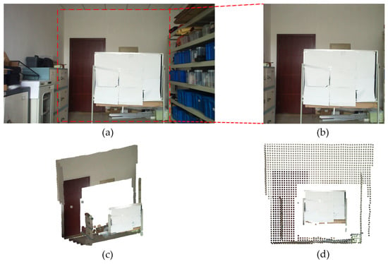
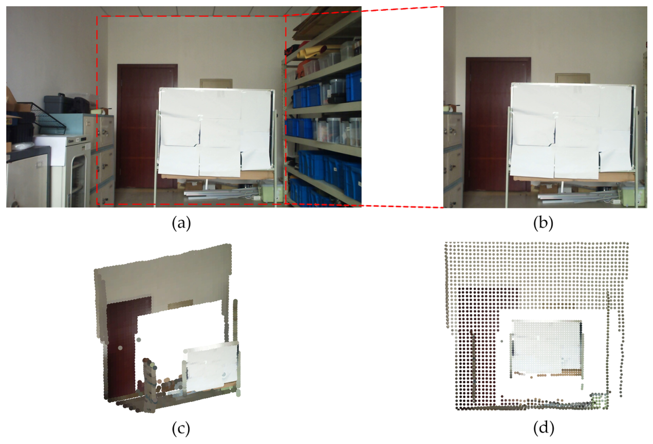
The intermediate 2500-point record was used only for the qualitative textured reconstruction and front-view point-cloud projection in Figure 10. For this visualization, the extrinsic pose was estimated once from the unperturbed 100-point calibration record using the Full P3LPnP objective and the rectified intrinsic matrix reported in Section 4.3. The resulting pose was then applied to the 2500-point record without re-optimization. Neither the 2500-point record nor its visualization was used in the quantitative comparisons reported in Table 6, Table 7 and Table 8. Figure 10 therefore provides a qualitative consistency illustration rather than an additional accuracy benchmark or an independent validation dataset.

Figure 10. Qualitative visualization obtained by transferring the unperturbed Full P3LPnP pose estimated from the 100-point calibration record to the 2500-point record without re-optimization: (a) Experimental scene. (b) Calibration scene. (c) Textured 3D reconstruction. (d) Front-view projection of the reconstructed point cloud.

Table 8. Constraint controls on the processed real-record geometry. Values are mean Euclidean re-projection error ± standard deviation across 30 paired perturbation instances.

Configuration	Active Term(s)	100-Point Sparse Error (px)	9900-Point Same-Session Error (px)
Point only	P	$0.416\pm 0.118$	$0.391\pm 0.115$
Point + exact duplicate	$P+P^{\ast }$ (same 3D/2D)	$0.419\pm 0.119$	$0.394\pm 0.116$
Point + endpoint position only	$P+E$	$0.408\pm 0.117$	$0.384\pm 0.114$
Point + length + direction	$P+L+D$ (no E)	$0.360\pm 0.118$	$0.342\pm 0.118$
Full P3LPnP	$P+L+D+E$	0.356 ± 0.118	0.338 ± 0.117

The asterisk denotes duplicated point observations with exactly the same 3D coordinates and 2D pixels as in the point term. These duplicates use the endpoint block grouping and weighting and add no new observation. Boldface identifies the Full P3LPnP method and its results.

The scope of this experiment was necessarily limited. The calibration and held-out correspondences originated from one LiDAR–camera system, one rigid mounting configuration, one scene, and one acquisition and processing chain. The 9900 held-out correspondences were not used by the pose optimizer and were disjoint from the 100 optimization correspondences at the record level, but they were neither statistically nor externally independent because they shared the same sensor, session, scene, and processing chain. Accordingly, the experiment supported real-record-based robustness, sparse-to-dense same-session transfer, and the constraint-control conclusions above. It did not establish multi-system, multi-session, or cross-scene generalizability.

6. Discussion

The experimental protocol evaluated front-end reconstruction, back-end pose estimation, and sparse-to-dense transfer separately. The matched front-end study showed that robust plane extraction and local purification are important before pose estimation, while the lattice study showed that PCA alone does not localize the checkerboard grid. In the controlled synthetic scenes, the known-size rigid-lattice fit consistently reconstructed unique co-planar nodes, whereas the extrema-and-snapping baseline could assign multiple provisional nodes to the same retained return.

The line-term results required a component-wise interpretation. Under the main independent-line protocol, the length term accounted for most of the measured improvement. The direction score changed the reported means by less than ${10}^{-5}$ when used alone and never entered the robust down-weighting regime under the default threshold. The endpoint-position term gave a smaller increment when it was based on separately perturbed line observations. When the same 3D and 2D boundary-point records were re-used exactly, the endpoint term was structured residual re-weighting and did not supply an independent observation. Thus, the evidence supported a conditional benefit from the full finite-segment formulation, not the claim that every line component was equally informative in every dataset.

Figure 6, Figure 7 and Figure 8 answer complementary questions. The 54-point experiment isolated deterioration of point localization while the line observations remained relatively reliable; P3LPnP was strongest there in translation. The 12-point joint-noise experiment was deliberately harder and showed competitive rather than uniformly best performance. The 12-point coherent-bias experiment produced the clearest clean-reference re-projection and translation advantage, while rotation remained a trade-off. Because the point counts and perturbation models differed, absolute error magnitudes were not compared across the full- and sparse-observation regimes. The synthetic tests also did not establish independence from camera resolution, focal length, or field of view, because those hardware variables were not changed.

The real-record results have a narrower interpretation. The lowest observed mean errors belonged to P3LPnP on both the 100-point reference and the 9900-point held-out set, but the paired confidence intervals against OPnPL included zero. The held-out observations were excluded from optimization, yet they originated from the same system, scene, session, and processing chain. The experiment therefore supports controlled same-system sparse-to-dense transfer and the constraint-control analysis, not statistically significant superiority over OPnPL or generalization to other rigs, sessions, scenes, distances, or poses.

Finally, validation of automatic lattice localization is currently limited to the synthetic scenes. The real-data implementation loads pre-associated image–3D records and source-configured contour indices rather than recovering the correspondence order from raw range returns. Fully automatic physical validation will require raw multi-pose and multi-distance acquisitions, an asymmetric target or another independently observable ordering cue, and tests on additional LiDAR–camera systems.

7. Conclusions

This paper presented P3LPnP, a plane-guided point-line method for target-based LiDAR–camera extrinsic calibration from sparse ranging observations. The front end combines robust plane reconstruction with explicit registration of a known-size rigid checkerboard lattice. The back end combines point re-projection, projected length, projected direction, and endpoint-position terms in a block-Huber objective. Block weights are updated in outer IRLS iterations and held fixed during each inner LM solve, with step acceptance based on the exact objective. Matched ablations showed that the plane-guided front end substantially improves plane and grid reconstruction, while the finite-segment objective reduces clean-reference re-projection and translation error relative to point-only optimization when separately generated line observations are available. The direction term was not a strong independent contributor under the reported configuration, and an endpoint term that exactly re-used point observations was interpreted as re-weighting. The two-regime synthetic evaluation further showed translation robustness under deteriorating point localization, competitive behavior under sparse joint random noise, and strong resistance to coherent feature bias in clean-reference re-projection and translation, without claiming uniform superiority in every metric. On the processed correspondence records from one physical system, P3LPnP gave the lowest observed mean re-projection errors on both the 100-point sparse reference and the 9900-point same-session held-out set. Its differences from OPnPL were not statistically significant under the present 30-run replay. The real-data conclusion was therefore limited to same-system consistency and controlled robustness. Future work will target raw-measurement correspondence recovery and independent multi-system, multi-session, multi-pose, and multi-distance validation.

References

- Huang, Y.H.; Lin, C.T. Indoor Localization Method for a Mobile Robot Using LiDAR and a Dual AprilTag. Electronics 2023, 12, 1023. [Google Scholar] [CrossRef] [Scilit]
- Mozzarelli, L.; Corno, M.; Savaresi, S.M. A Comparative Experimental Study of LiDAR, Camera, and LiDAR-Camera Localization Algorithms for Autonomous Mobile Robots on Urban Sidewalks. In Proceedings of the 2023 IEEE Conference on Control Technology and Applications (CCTA), Bridgetown, Barbados, 16–18 August 2023; pp. 53–58. [Google Scholar] [CrossRef] [Scilit]
- Maslim, R.; Ramanathan, M.; Garg, N.P.; Ang, W.T. Position Based Camera-2D LiDAR Fusion and Person Following for Mobile Robots. In Proceedings of the 2025 International Conference On Rehabilitation Robotics (ICORR), Chicago, IL, USA, 12–16 May 2025; pp. 314–319. [Google Scholar] [CrossRef] [Scilit] [PubMed]
- Liu, H.; Wu, C.; Wang, H. Real Time Object Detection Using LiDAR and Camera Fusion for Autonomous Driving. Sci. Rep. 2023, 13, 8056. [Google Scholar] [CrossRef] [Scilit] [PubMed]
- Xu, X.; Dong, S.; Xu, T.; Ding, L.; Wang, J.; Jiang, P.; Song, L.; Li, J. FusionRCNN: LiDAR-Camera Fusion for Two-Stage 3D Object Detection. Remote Sens. 2023, 15, 1839. [Google Scholar] [CrossRef] [Scilit]
- An, P.; Ma, T.; Yu, K.; Fang, B.; Zhang, J.; Fu, W.; Ma, J. Geometric Calibration for LiDAR-Camera System Fusing 3D-2D and 3D-3D Point Correspondences. Opt. Express 2020, 28, 2122–2141. [Google Scholar] [CrossRef] [Scilit] [PubMed]
- An, P.; Gao, Y.; Ma, T.; Yu, K.; Fang, B.; Zhang, J.; Ma, J. LiDAR-Camera System Extrinsic Calibration by Establishing Virtual Point Correspondences from Pseudo Calibration Objects. Opt. Express 2020, 28, 18261–18282. [Google Scholar] [CrossRef] [Scilit] [PubMed]
- Geiger, A.; Moosmann, F.; Car, O.; Schuster, B. Automatic Camera and Range Sensor Calibration Using a Single Shot. In Proceedings of the 2012 IEEE International Conference on Robotics and Automation, Saint Paul, MN, USA, 14–18 May 2012; pp. 3936–3943. [Google Scholar] [CrossRef] [Scilit]
- Li, X.; Xiao, Y.; Wang, B.; Ren, H.; Zhang, Y.; Ji, J. Automatic Targetless LiDAR-Camera Calibration: A Survey. Artif. Intell. Rev. 2023, 56, 9949–9987. [Google Scholar] [CrossRef] [Scilit]
- Lee, X.; Wang, C.; Luo, Z.; Li, S. Optical design of a new folding scanning system in MEMS-based lidar. Opt. Laser Technol. 2020, 125, 106013. [Google Scholar] [CrossRef] [Scilit]
- Duma, V.F.; Dimb, A.L. Exact Scan Patterns of Rotational Risley Prisms Obtained with a Graphical Method: Multi-Parameter Analysis and Design. Appl. Sci. 2021, 11, 8451. [Google Scholar] [CrossRef] [Scilit]
- Li, A.; Liu, X.; Sun, J.; Lu, Z. Risley-prism-based multi-beam scanning LiDAR for high-resolution three-dimensional imaging. Opt. Lasers Eng. 2022, 150, 106836. [Google Scholar] [CrossRef] [Scilit]
- Liu, X.; Li, A.; Jiang, X.; Yang, H.; Li, Y. Cascaded-prism multi-mode beam scanning method for three-dimensional imaging lidar. Appl. Opt. 2024, 63, 5670–5678. [Google Scholar] [CrossRef] [Scilit]
- Lepetit, V.; Moreno-Noguer, F.; Fua, P. EPnP: An Accurate O(n) Solution to the PnP Problem. Int. J. Comput. Vis. 2009, 81, 155–166. [Google Scholar] [CrossRef] [Scilit]
- Hesch, J.A.; Roumeliotis, S.I. A Direct Least-Squares (DLS) Method for PnP. In Proceedings of the 2011 IEEE International Conference on Computer Vision, Barcelona, Spain, 6–13 November 2011; pp. 383–390. [Google Scholar] [CrossRef] [Scilit]
- Terzakis, G.; Lourakis, M. A Consistently Fast and Globally Optimal Solution to the Perspective-n-Point Problem. In Proceedings of the European Conference on Computer Vision, Glasgow, UK, 23–28 August 2020; pp. 478–494. [Google Scholar] [CrossRef] [Scilit]
- Yi, H.; Liu, B.; Zhao, B.; Liu, E. Extrinsic Calibration for LiDAR-Camera Systems Using Direct 3D-2D Correspondences. Remote Sens. 2022, 14, 6082. [Google Scholar] [CrossRef] [Scilit]
- Jeong, S.; Kim, S.; Kim, J.; Kim, M. O3 LiDAR-Camera Calibration: One-Shot, One-Target and Overcoming LiDAR Limitations. IEEE Sens. J. 2024, 24, 18659–18671. [Google Scholar] [CrossRef] [Scilit]
- Xu, X.; Zhang, L.; Yang, J.; Liu, C.; Xiong, Y.; Luo, M.; Tan, Z.; Liu, B. LiDAR–Camera Calibration Method Based on Ranging Statistical Characteristics and Improved RANSAC Algorithm. Robot. Auton. Syst. 2021, 141, 103776. [Google Scholar] [CrossRef] [Scilit]
- Ou, N.; Cai, H.; Yang, J.; Wang, J. Targetless Extrinsic Calibration of Camera and Low-Resolution 3D LiDAR. IEEE Sens. J. 2023, 23, 10889–10899. [Google Scholar] [CrossRef] [Scilit]
- Lai, Z.; Wang, Y.; Guo, S.; Meng, X.; Li, J.; Li, W.; Han, S. Laser Reflectance Feature Assisted Accurate Extrinsic Calibration for Non-Repetitive Scanning LiDAR and Camera Systems. Opt. Express 2022, 30, 16242–16263. [Google Scholar] [CrossRef] [Scilit] [PubMed]
- Sim, S.; Sock, J.; Kwak, K. Indirect Correspondence-Based Robust Extrinsic Calibration of LiDAR and Camera. Sensors 2016, 16, 933. [Google Scholar] [CrossRef] [Scilit] [PubMed]
- Vakhitov, A.; Ferraz, L.; Agudo, A.; Moreno-Noguer, F. Uncertainty-Aware Camera Pose Estimation from Points and Lines. In Proceedings of the IEEE/CVF Conference on Computer Vision and Pattern Recognition (CVPR), Nashville, TN, USA, 20–25 June 2021; pp. 4657–4666. [Google Scholar] [CrossRef] [Scilit]
- Bai, Z.; Jiang, G.; Xu, A. LiDAR-Camera Calibration Using Line Correspondences. Sensors 2020, 20, 6319. [Google Scholar] [CrossRef] [Scilit] [PubMed]
- Vakhitov, A.; Funke, J.; Moreno-Noguer, F. Accurate and Linear Time Pose Estimation from Points and Lines. In Proceedings of the European Conference on Computer Vision, Amsterdam, The Netherlands, 11–14 October 2016; pp. 583–599. [Google Scholar] [CrossRef] [Scilit]
- Wang, W.; Sakurada, K.; Kawaguchi, N. Reflectance Intensity Assisted Automatic and Accurate Extrinsic Calibration of 3D LiDAR and Panoramic Camera Using a Printed Chessboard. Remote Sens. 2017, 9, 851. [Google Scholar] [CrossRef] [Scilit]
- Chen, H.; Wang, P.; Wang, F.; Tian, W.; Xiong, L.; Li, H. EPro-PnP: Generalized End-to-End Probabilistic Perspective-n-Points for Monocular Object Pose Estimation. In Proceedings of the IEEE/CVF Conference on Computer Vision and Pattern Recognition (CVPR), New Orleans, LA, USA, 18–24 June 2022; pp. 2781–2790. [Google Scholar] [CrossRef] [Scilit]
- Yi, H.; Liu, B.; Zhao, B.; Liu, E. Outliers Rejection for Robust Camera Pose Estimation Using Graduated Non-Convexity. IET Comput. Vis. 2025, 19, e12330. [Google Scholar] [CrossRef] [Scilit]
- Xie, X.; Zou, D. Depth-Based Efficient PnP: A Rapid and Accurate Method for Camera Pose Estimation. IEEE Robot. Autom. Lett. 2024, 9, 9287–9294. [Google Scholar] [CrossRef] [Scilit]
- Nguyen, A.D.; Nguyen, T.M.; Yoo, M. Improvement to LiDAR-Camera Extrinsic Calibration by Using 3D-3D Correspondences. Optik 2022, 259, 168917. [Google Scholar] [CrossRef] [Scilit]
- Zhang, Q.; Pless, R. Extrinsic Calibration of a Camera and Laser Range Finder (Improves Camera Calibration). In Proceedings of the 2004 IEEE/RSJ International Conference on Intelligent Robots and Systems (IROS), Sendai, Japan, 28 September–2 October 2004; Volume 3, pp. 2301–2306. [Google Scholar] [CrossRef] [Scilit]
- Gong, X.; Lin, Y.; Liu, J. 3D LiDAR-Camera Extrinsic Calibration Using an Arbitrary Trihedron. Sensors 2013, 13, 1902–1918. [Google Scholar] [CrossRef] [Scilit] [PubMed]
- Mirzaei, F.M.; Roumeliotis, S.I. Globally Optimal Pose Estimation from Line Correspondences. In Proceedings of the 2011 IEEE International Conference on Robotics and Automation, Shanghai, China, 9–13 May 2011; pp. 5581–5588. [Google Scholar] [CrossRef] [Scilit]
- Xu, C.; Zhang, L.; Cheng, L.; Koch, R. Pose Estimation from Line Correspondences: A Complete Analysis and a Series of Solutions. IEEE Trans. Pattern Anal. Mach. Intell. 2017, 39, 1209–1222. [Google Scholar] [CrossRef] [Scilit] [PubMed]
- Pusztai, Z.; Hajder, L. Accurate Calibration of LiDAR-Camera Systems Using Ordinary Boxes. In Proceedings of the 2017 IEEE International Conference on Computer Vision Workshops (ICCVW), Venice, Italy, 22–29 October 2017; pp. 394–402. [Google Scholar] [CrossRef] [Scilit]
- Kim, E.s.; Park, S.Y. Extrinsic Calibration between Camera and LiDAR Sensors by Matching Multiple 3D Planes. Sensors 2020, 20, 52. [Google Scholar] [CrossRef] [Scilit] [PubMed]
- Munoz-Banon, M.A.; Candelas, F.A.; Torres, F. Targetless Camera-LiDAR Calibration in Unstructured Environments. IEEE Access 2020, 8, 143692–143705. [Google Scholar] [CrossRef] [Scilit]
- Yin, J.; Yan, F.; Liu, Y.; Zhuang, Y. Automatic and Targetless LiDAR-Camera Extrinsic Calibration Using Edge Alignment. IEEE Sens. J. 2023, 23, 19871–19880. [Google Scholar] [CrossRef] [Scilit]
- Jin, S.; Ma, C.; Gao, Y.; Hui, F.; Zhao, X. Roadside Camera-LiDAR Calibration Without Annotation. IEEE Sens. J. 2024, 24, 37654–37665. [Google Scholar] [CrossRef] [Scilit]
- Pan, F.; Wang, W. CalibOnline: Online Detection and Calibration of Extrinsic Parameters Between LiDAR and Monocular Camera. IEEE Sens. J. 2025, 25, 20323–20332. [Google Scholar] [CrossRef] [Scilit]
- Zhang, B.; Li, M.; Liu, S.; Liu, W.; Tian, Y.; Li, Q.; Wu, J. PCDC-Cal: Real-Time Targetless Roadside LiDAR-Camera Extrinsic Calibration via Point-Cloud Directional Consistency. IEEE Sens. J. 2025, 25, 44680–44696. [Google Scholar] [CrossRef] [Scilit]
- Fischler, M.A.; Bolles, R.C. Random Sample Consensus: A Paradigm for Model Fitting with Applications to Image Analysis and Automated Cartography. Commun. ACM 1981, 24, 381–395. [Google Scholar] [CrossRef] [Scilit]
- Ester, M.; Kriegel, H.P.; Sander, J.; Xu, X. A Density-Based Algorithm for Discovering Clusters in Large Spatial Databases with Noise. In Proceedings of the Second International Conference on Knowledge Discovery and Data Mining, Portland, OR, USA, 2–4 August 1996; pp. 226–231. [Google Scholar]
- Pearson, K. On Lines and Planes of Closest Fit to Systems of Points in Space. Lond. Edinb. Dublin Philos. Mag. J. Sci. 1901, 2, 559–572. [Google Scholar] [CrossRef] [Scilit]
- Marquardt, D.W. An Algorithm for Least-Squares Estimation of Nonlinear Parameters. J. Soc. Ind. Appl. Math. 1963, 11, 431–441. [Google Scholar] [CrossRef] [Scilit]
Disclaimer/Publisher’s Note: The statements, opinions and data contained in all publications are solely those of the individual author(s) and contributor(s) and not of MDPI and/or the editor(s). MDPI and/or the editor(s) disclaim responsibility for any injury to people or property resulting from any ideas, methods, instructions or products referred to in the content. |
© 2026 by the authors. Licensee MDPI, Basel, Switzerland. This article is an open access article distributed under the terms and conditions of the Creative Commons Attribution (CC BY) license.