DAVis-Net: A Dual-Attention Deep Supervision Framework for Reliable Retinal OCT Image Classification with Integrated Explainability and Uncertainty Quantification

Abstract

Classification accuracy in retinal optical coherence tomography (OCT) alone does not establish whether a model is reliable or whether to refer to a specialist. To address this, we propose DAVis-Net, a VGG16-based architecture that is equipped with two Convolutional Block Attention Modules (CBAMs), an auxiliary deep-supervision head, and an integrated reliability framework that includes Monte Carlo Dropout uncertainty estimation, model calibration, split conformal prediction, and quantitative multi-method attribution analysis. DAVis-Net has achieved a cross-validated accuracy of 98.02% ± 0.12% on the four classes of OCT (CNV, DME, DRUSEN, NORMAL), statistically significantly higher than the VGG16 baseline in a matched-fold paired comparison (accuracy: p = 0.023; macro-F1: p = 0.004), with the highest gain on the hardest class (DRUSEN F1 +4.57 pp). Joint correlation analysis showed strong redundancy between predictive entropy and conformal set size (r = 0.67–0.78) across all classes, and a near zero linear correlation between both of these and a geometric proxy for spatial attention placement (|r| < 0.08), suggesting that, as captured by this central-region localization proxy, distributional uncertainty and spatial attention placement may reflect largely distinct reliability dimensions. A composite Trust/Refer triage rule achieved an accuracy of 99.76% on the 73.9% of cases it retained. All reported figures are internal estimates derived from a single dataset at the image-level, and multi-center validation is still required. The results show that the multi-dimensional reliability assessment is a more informative characterization of a medical image classifier than accuracy alone.

1. Introduction

Optical coherence tomography (OCT) is a non-invasive imaging technique that achieves micrometer-scale axial resolution [1], and produces high-resolution cross-sectional retinal images. The presence of focal extracellular deposits beneath the retinal pigment epithelium (RPE), called DRUSEN, is an early indicator of Age-related Macular Degeneration (AMD) and must be distinguished from choroidal neovascularization (CNV) and diabetic macular edema (DME) [2,3]. The timing of sight-preserving intervention is directly related to the accuracy of OCT B-scan interpretation, and the number of clinical OCT scans has increased more rapidly than the number of trained graders [4], as these conditions can progress irreversibly.

Convolutional neural networks have met the accuracy requirement quite successfully. Since then, headline accuracy levels have climbed to 96–99% with Inception V3 [5] and further advances with VGG16 [6,7] and ResNet-50 [8], attention-augmented CNNs [9,10,11], fusion networks [12], lesion-aware architectures [13] and transformer-based models [14,15,16]. In terms of raw accuracy, four-class OCT classification is largely considered solved.

But reliability has not kept pace. A model that is only deterministic in its output does not provide any hint to the clinician of when to distrust its predictions [4], and softmax probabilities are known to be poorly calibrated [17]. There are three identified gaps. First, explainability evaluations [18,19,20] remain largely qualitative—heatmaps are examined but rarely subjected to faithfulness tests such as confidence drops or debiased perturbation frameworks [21,22,23]. Second, uncertainty estimation [24,25] and conformal prediction [26,27] have each been used in medical imaging. However, their class-specific behavior on OCT data remains uncharacterized, and it is unclear whether these signals are redundant with or complementary to spatial explanation quality. Third, no existing OCT framework unites classification, quantitative explainability, uncertainty estimation, calibration, and conformal prediction in one pipeline and examines the relationships among the signals these components generate. A classifier with 98% accuracy cannot then serve as the basis for per-case escalation decisions. Although the components are available individually, how they work together for the same predictions is unknown, and the implications are not theoretical, as the drop in FN-OCT accuracy from 98.5% for in-distribution samples to 81% on out-of-distribution samples demonstrates [12].

This study aims to fill these gaps in three ways:

(1)

To preserve the mid-level spatial features that are crucial in focal retinal pathologies, we propose DAVis-Net, an architecture based on VGG16 with two CBAM blocks and an auxiliary deep-supervision head.

(2)

We design an integrated framework that uses MC Dropout uncertainty estimation, post hoc temperature scaling, split conformal prediction, and quantitative multi-method explainability (Grad-CAM, Grad-CAM++, Score-CAM).

(3)

We perform a joint correlation analysis that reveals that distributional uncertainty and a geometric measure of spatial explanation placement exhibit near-zero correlation, and operationalize this as a Trust/Refer triage rule.

The remainder of this article is organized as follows. Section 2 discusses related work and provides a summary. Section 3 describes the dataset, the DAVis-Net architecture, and analytical methods such as explainability, uncertainty estimation, calibration, and conformal prediction. Section 4 presents the results of the analytical methods. Section 5 covers the main findings, limitations, and future directions, while Section 6 provides the conclusion.

2. Literature Review

2.1. CNN and Attention-Based OCT Classification

Kermany et al. [5] set up the four-class OCT benchmark based on Inception V3 transfer learning on more than 108,000 B-scans. To increase the evaluation rigor, Jaimes et al. [7] used 10-fold Monte Carlo cross-validation on a balanced VGG16 subset (95.19%), and Akula et al. [8] enforced patient-level splits with ResNet-50 (97.83%). The attention-based extensions are CBAM integration by Novely et al. [10] (96.31% on OCT-C8), the parallel global attention block of Huang et al. [11] tested on an external scanner cohort, and the FN-OCT fusion network of Ai et al. [12] with 98.5% internally and 81–92% on external validation—a direct motivation for the reliability-centered framing of the present work. In contrast, Fang et al. [13] trained attention maps on lesion regions annotated by ophthalmologists to explicitly enforce clinical faithfulness. Transformer-based methods have also achieved higher accuracy: He et al. [14] used Swin Transformer (99.80%), Li et al. [15] employed Swin Transformer V2 (99.90%), and Upmanu et al. [16] proposed an explainable ViT (98.84% under 10-fold CV). None of these contains uncertainty quantification or conformal prediction, though. The DRUSEN class is the most difficult to classify across all architectures [5,7,10], due to the natural overlap between small sub-RPE elevations, incipient neovascular change, and normal retinal variation [2,3].

2.2. Explainability in Medical Imaging

Post hoc spatial explanations of CNN decisions include Grad-CAM [18], Grad-CAM++ [19], and Score-CAM [20], with increasingly less dependence on gradients; computational details are provided in Section 3.5. These methods are now frequently employed in OCT studies [7,14,16] but are mostly used qualitatively. Singh et al. [21] and Yavari et al. [22] quantitatively compared attribution methods for ophthalmic diagnosis, demonstrating that the quality of attribution is not guaranteed off-the-shelf. Rong et al. [23] suggested the ROAD framework for debiased imputation to overcome out-of-distribution artifacts of standard insertion/deletion metrics. Commonly, high classification accuracy does not translate into clinically faithful localization.

2.3. Uncertainty, Calibration, and Conformal Prediction

Gal and Ghahramani [24] demonstrated that MC Dropout yields an approximate Bayesian uncertainty using current dropout architectures. Kurz et al. [25] systematically reviewed 22 studies on uncertainty in medical imaging, and called for integration into collaborative human–machine workflows. Faghani et al. [17] highlighted the gap between uncertainty methods and clinical deployment under distribution shift. Conformal prediction offers distribution-free coverage guarantees that hold for finite samples [26]. It has been applied to inherited retinal disease classification at Moorfields Eye Hospital [27]. To tighten prediction sets, Hirsch and Goldberger [28] proposed per-sample adaptive thresholds, and Borah and Singh [29] used ResNet34 and EfficientNetB4 with conformal prediction on four medical datasets (91.17% on OCT). They also included a fallback rule for empty sets.

2.4. Research Gaps and Motivation

There have been significant advances in classification accuracy, attribution-based explainability, uncertainty estimation, and conformal prediction, independently. Their integration is missing: high-accuracy studies do not test reliability [8,10,12]; explainability studies provide qualitative heat maps, but without faithfulness testing [14,16]; uncertainty and conformal studies do not consider class-specific OCT behavior and its relation to the quality of the spatial explanation [17,25]. As far as we know, no earlier research has determined whether explainability and uncertainty signals are redundant or complement each other. The present work answers the question directly by integrating all four components in one framework and doing per-class correlation analysis. Existing studies are summarized in Table 1.

Table 1. Representative model architectures used for retinal OCT classification.

Study	Model/Architecture	Key Contributions
Kermany et al. [5].	Inception V3	Established the widely used 4-class OCT benchmark.
Jaimes et al. [7]; Yavari et al. [22].	Modified VGG16	CNN-based OCT classification and attribution analysis.
Akula et al. [8].	ResNet-50	Transfer learning and feature extraction.
Novely et al. [10]; Huang et al. [11]; Ai et al. [12]; Fang et al. [13].	CNN + Attention	Incorporation of channel/spatial or lesion-aware attention to improve feature representations.
He et al. [14]; Li et al. [15]; Upmanu et al. [16].	Swin Transformer; Vision Transformer (ViT)	Transformer-based OCT classification with post hoc visual explainability.
Singh et al. [21].	Multiple Attribution Models	Quantitative evaluation of attribution methods in ophthalmic imaging.
Ghoshal et al. [27]; Hirsch & Goldberger [28]; Borah & Singh [29].	Conformal Prediction Models	Prediction-set generation and uncertainty-aware decision support.
DAVis-Net (ours)	VGG16 + 2x CBAM + Deep Supervision	Attention-enhanced CNN with integrated reliability framework.

3. Materials and Methods

3.1. Dataset

We utilized a publicly accessible redistribution of the Kermany et al. [5] retinal OCT collection. The distributed partition was created by combining all images from the original collection and then re-splitting them at random by class. This procedure is image-based, not patient-based, and therefore the same B-scans may be seen in multiple partitions. The dataset was pre-partitioned into a train/validation/test split of 70:15:15.

The dataset comprises retinal OCT B-scan images across four categories: choroidal neovascularization (CNV), diabetic macular edema (DME), DRUSEN deposits (DRUSEN), and healthy retina (NORMAL). The split comprises 58,697 training images, 12,662 validation images, and 12,650 test images. DRUSEN samples are about 4.3 times fewer than CNV, making it the minority class. We addressed class imbalance at two levels. At the data level, we used image augmentation on DRUSEN samples. We used the resulting training distribution to compute inverse-frequency class weights and applied them to both the main focal loss and the auxiliary weighted cross-entropy loss. Table 2 shows the full dataset composition. No images were excluded, filtered, or removed during the preprocessing. We have used the publicly shared cohort as is.

Table 2. Dataset composition by class and partition.

Class	Train	Train (Augmented)	Validation	Test	Total	Class Weight
CNV	26,080	26,080	5616	5614	37,310	0.621
DME	8043	8043	1737	1734	11,514	2.013
DRUSEN	6073	12,146	1327	1321	8721	1.333
NORMAL	18,501	18,501	3982	3981	26,464	0.875

All images are resized to 224 × 224, converted to RGB, and normalized with ImageNet channel means and std. We did not implement generative and interpolation-based oversampling, such as SMOTE and GAN-based synthesis, because the low contrast and small size of the sub-RPE elevation of DRUSEN are most susceptible to corruption. However, we corrected this with augmentation strategies such as horizontal flipping, ±10° image rotations, ±15% brightness/contrast jitter, and Gaussian noise (σ = 0.02), as well as inverse-frequency loss weighting techniques and the architectural changes described in Section 3.4.

3.2. Computational Environment

We conducted all experiments on the computational environment offered by the Kaggle platform using a single NVIDIA Tesla T4 GPU with 16 GB VRAM. The deep learning models were implemented using PyTorch 2.10.0 with CUDA 12.8 on Python 3.12.13. We performed statistical analyses using NumPy 2.0.2, Scikit-Learn 1.6.1, and Pandas 2.3.3. The figures in this study were created using Matplotlib 3.10.0 and Seaborn 0.13.2. A fixed random seed of 42 was used throughout the study, with cuDNN set to deterministic mode.

3.3. Baseline Models and Image Ablation Study

To ensure the backbone selection was based on empirical evidence rather than random choice, we screened five CNN architectures before making any architectural changes: VGG16 [6], ResNet-50 [30], DenseNet121 [31], Xception [32], and EfficientNetB3 [33]. The same classification head (Global average pooling, Dropout, Dense layer with 256 units and ReLU activation, Dropout, Dense layer with 4 units and softmax activation) was used for each backbone, which was trained with the same augmentation and controlled by the same callbacks (early stopping on validation loss with patience of 5; learning rate reduction on plateau with factor 0.2 and patience 2). All models were first head-trained to a similar degree, and then the backbone was fine-tuned, so that the only difference between the models is the backbone.

Table 3 presents the screening results. VGG16 achieved the best overall accuracy (97.16%) and, most importantly, the best F1 score (95.95%) among the five architectures. Relative class difficulty was the same across all backbones, with DRUSEN being the lowest-scoring class for all models, ranging from DenseNet121’s 68.50% to VGG16’s 90.67%. This consistency indicates that the DRUSEN class is inherently difficult in the classification task and is not due to any specific model. Based on this comparison, we further validated VGG16 using 5-fold cross-validation, achieving a mean accuracy of 97.58% ± 0.22% across folds. We then selected VGG16 as the backbone for DAVis-Net.

Table 3. CNN backbone screening results.

CNN Backbone	Accuracy (%)	Macro-F1 (%)	Inference Time (ms)
VGG16	97.16	95.95	3.898
ResNet-50	93.68	90.48	3.071
DenseNet121	91.28	86.20	3.703
Xception	94.79	92.51	3.935
EfficientNetB3	93.41	90.08	3.405

We performed an image ablation study on the VGG16 backbone, testing four preprocessing variants: no enhancement, CLAHE, CLAHE with gamma correction, and CLAHE with gamma correction and unsharp masking. The performance of each variant is shown in Table 4. The best variant (CLAHE with gamma) only improved DRUSEN F1 by 0.0023 over the baseline.

Table 4. Image enhancement ablation results.

Variant	Accuracy (%)	Macro-F1 (%)	Drusen F1 (%)
A: Baseline (no enhancement)	96.98	95.69	90.67
B: CLAHE	97.00	95.75	90.82
C: CLAHE + Gamma	97.09	95.84	90.90
D: CLAHE + Gamma + Unsharp	96.88	95.54	90.20

The entire three-stage enhancement chain had a negative impact. We interpret this outcome as follows: Contrast-enhancement techniques like CLAHE consider the local intensity distribution; they are most useful when the discriminative signal exists but is not clearly distinguishable from the background intensity. This degradation was also observed with unsharp masking, where the amplification of high frequencies not only increases the sub-RPE elevation that is the basis of a DRUSEN deposit, but also the speckle noise characteristic of OCT acquisition; and, since speckle and small DRUSEN lie in overlapping spatial frequency bands, the operation increases the noise floor at least as much as the signal. These considerations led us to develop architecture-level and loss-level interventions that operate on the learned representation rather than directly modifying the input, yielding larger gains, as reported in Section 4.1.

3.4. DAVis-Net Architecture

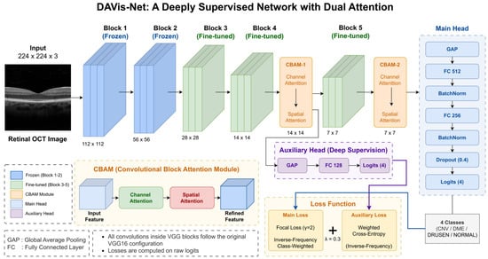
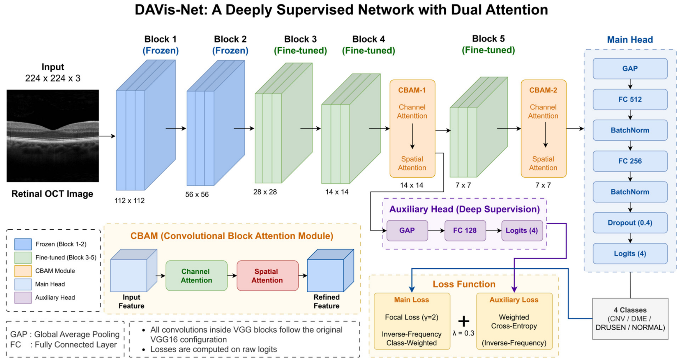
DAVis-Net makes two targeted modifications to the VGG16 backbone to improve the representation of morphologically subtle pathology, whose spatial signature may be lost in the deeper, more heavily pooled layers of the network. The architecture is depicted in Figure 1, which shows the five VGG16 blocks, with Blocks 1 and 2 frozen and Blocks 3 through 5 fine-tuned, the two CBAMs after Blocks 4 and 5, the auxiliary classification head branched from the CBAM-1 features, the main classification head branched from the CBAM-2 features, and the two loss terms that are jointly optimized. The figure can be followed from the beginning of the forward pass, and the dual-head supervision scheme can be understood at a glance.

Figure 1. Proposed DAVis-Net architecture.

The first modification is the addition of two Convolutional Block Attention Modules [9] after Block 4 and Block 5, which are called CBAM-1 and CBAM-2, respectively. The two attentions, channel and spatial, are applied to each module. Channel attention is computed as parallel average and max pooling and then passed through the same multi-layer perceptron as shown in Equation (1) with a reduction ratio r = 8:

$$M_c\left(F\right)=\sigma \left(\mathrm{M}\mathrm{L}\mathrm{P}\left(\mathrm{A}\mathrm{v}\mathrm{g}\mathrm{P}\mathrm{o}\mathrm{o}\mathrm{l}\left(F\right)\right)+\mathrm{M}\mathrm{L}\mathrm{P}\left(\mathrm{M}\mathrm{a}\mathrm{x}\mathrm{P}\mathrm{o}\mathrm{o}\mathrm{l}\left(F\right)\right)\right)$$

(1)

Spatial attention, as illustrated in Equation (2), then enhances this by pooling across the channel dimension and convolving a single time step with a $7\times 7$ kernel to identify informative spatial positions:

$$M_s\left(F^{\prime }\right)=\sigma \left(f^{7\times 7}\left(\left[\mathrm{A}\mathrm{v}\mathrm{g}\mathrm{P}\mathrm{o}\mathrm{o}{\mathrm{l}}_{\mathrm{c}}\left(F^{\prime }\right);\mathrm{M}\mathrm{a}\mathrm{x}\mathrm{P}\mathrm{o}\mathrm{o}{\mathrm{l}}_{\mathrm{c}}\left(F^{\prime }\right)\right]\right)\right)$$

(2)

The two attention maps are then applied sequentially by element-wise multiplication to get the refined feature map represented in Equation (3):

$$F^{\prime }=M_c\left(F\right)\otimes F, F^{″}=M_s\left(F^{\prime }\right)\otimes F^{\prime }$$

(3)

where $F\in {\mathbb{R}}^{C\times H\times W}$ is the input feature map, $M_c\left(·\right)$ and $M_s\left(·\right)$ are the channel and spatial attention maps from Equations (1) and (2). $F^{\prime }$ and $F^{″}$ are the channel-refined and spatially refined feature maps, and the $\otimes$ operator represents the Hadamard product. The rationale for the dual placement is based on spatial-resolution-driven considerations. In most previous CBAM-based OCT studies [10], an extra attention module is added to the last convolutional block, and the feature maps are already shrunk to $7\times 7$ spatial resolution. The small spatial extent of a small DRUSEN deposit can be smeared over just a few activation sites at this depth. CBAM-1 also improves the Block 4 features at $14\times 14$ resolution while maintaining fine spatial details, giving the network two receptive-field scales to focus on diagnostically relevant areas.

The second modification is an auxiliary head directly attached to the CBAM-1 features, which consists of Global average pooling, a Dense layer with 128 units and ReLU activation, and a Dense output layer with 4 units and softmax activation. This auxiliary head is trained with its own classification loss, forcing the mid-level features to contain class-discriminative information instead of just being a channel to deeper layers. Direct supervision allows minority-relevant features to reach the classification stage, since they are less strongly represented in the middle layers than in the deepest layers. The main classification head includes these layers: CBAM-2, Global average pooling, a Dense layer with 512 units and ReLU activation, Batch normalization, another Dense layer with 256 units followed by ReLU, Batch normalization, Dropout at 0.4, and a final Dense layer with 4 units using softmax activation to produce class probabilities.

The total loss ${\mathcal{L}}_{total}$ is calculated as shown in Equation (4). Both heads are trained together with a common objective:

$${\mathcal{L}}_{total}={\mathcal{L}}_{main}+\lambda {\mathcal{L}}_{aux}$$

(4)

where $\lambda$ = 0.3 is a compromise between the auxiliary contribution and the main objective. The main head is optimized with focal loss (see Equation (5)), which down-weights easy examples and focuses learning on hard ones, and with inverse-frequency class weights ${\alpha }_c$:

$${\mathcal{L}}_{focal}=-{\alpha }_c{\left(1-p_t\right)}^{\gamma }\log \left(p_t\right)$$

(5)

Here, $\gamma$ = 2 is the focusing parameter, and $p_t$ is the predicted probability of the true class. The auxiliary head is trained with standard cross-entropy with the same inverse-frequency weights. Table 5a summarizes all hyperparameters that control the architecture and training.

Table 5. (a) DAVis-Net hyperparameter configuration; (b) Data partition usage summary.

(a) DAVis-Net Hyperparameter Configuration
Parameter	Value
Auxiliary loss weight ($\lambda$)	0.3
Focal loss ($\gamma$)	2.0
Dropout rate	0.4
Optimizer	AdamW; Weight decay $1\times {10}^{-4}$
Learning rate	Backbone: $5\times {10}^{-4}$ CBAM and Heads: $5\times {10}^{-5}$
LR schedule	ReduceLROnPlateau on validation accuracy; factor 0.5, patience 3, min $1\times {10}^{-6}$
Gradient clipping	Max ${\mathcal{l}}_2$ norm 1.0
Batch size	32
Maximum epochs	40
Early stopping	Validation accuracy; patience 7
Random seed	42
(b) Data Partition Usage Summary
Partition	Size	Purpose	Section(s)
Training set	Originally 58,697 64,770—DRUSEN augmented	CNN backbone screening; Image ablation study; Final model training.	Section 3.3 and Section 3.4
Validation set	12,662	CNN backbone selection; Early stopping for final model; Temperature-scale fitting ($T^{\ast }$).	Section 3.3, Section 3.4 and Section 3.6
Training + Validation (pooled)	71,359	5-fold cross-validation (VGG16 vs. DAVis-Net comparison).	Section 3.4
Test set	12,650	Final model evaluation; Reliability evaluation.	Section 4.1, Section 4.3, Section 4.4, Section 4.5, Section 4.6 and Section 4.7
Conformal calibration subset	7588 (60% of test set)	Compute nonconformity threshold $\widehat{q}$.	Section 3.7 and Section 4.5
Conformal evaluation subset	5062 (40% of test set)	Reporting final coverage; Trust/Refer performance; Joint correlation analysis.	Section 3.7, Section 4.5, Section 4.6 and Section 4.7

$T^{\ast }$ denotes the temperature used in Equation (8).

Table 5b summarizes each data partition utilized in this study, detailing its size and the decisions it informed, thereby ensuring that the data flow underlying both evaluation protocols described below remains unambiguous.

We have used two evaluation protocols. The baseline VGG16 and DAVis-Net were compared using stratified 5-fold cross-validation (scikit-learn StratifiedKFold, class-stratified, fixed random seed 42) on the pooled training and validation partitions (N = 71,359) to assess classification performance. Augmentation was applied after the fold split to the training sets of each fold, but not to the combined training set before the split, to avoid having augmented versions of a given base image in both the training and validation sets of a fold. A single instance of DAVis-Net was then trained independently on the original training partition, using the validation partition for early-stopping monitoring, and evaluated on the held-out test partition. The same model was used for the reliability analysis (Section 4.3, Section 4.4, Section 4.5, Section 4.6 and Section 4.7). Performing the reliability analysis on the five models was computationally too expensive, and ensembling them would independently decrease the predictive entropy. For these reasons, we have used a single trained instance for the entire downstream pipeline.

The classification performance was assessed using metrics such as accuracy, precision, recall, and F1 score for each class, along with macro-averages. Calibration quality was evaluated through the Expected calibration error (ECE), Maximum calibration error (MCE), and Brier score. Uncertainty was quantified using predictive entropy, variation ratio, mutual information, and mean confidence.

3.5. Explainability Analysis

To evaluate the spatial consistency of DAVis-Net’s predictions with diagnostically relevant retinal regions, three post hoc attribution techniques were used: Grad-CAM, Grad-CAM++, and Score-CAM [18,19,20]. By employing three methods instead of one, the dependence on any particular attribution algorithm is avoided, and inter-method consistency can be directly evaluated. Grad-CAM produces heat maps that highlight class-specific features by combining the target-class gradients with globally pooled feature maps. Grad-CAM++ enhances this method with pixel-wise weighting of positive gradients for finer localization, while Score-CAM eliminates the use of gradients, instead assigning weights based on the model’s confidence response for each activation map in channel-masked inputs. For all test samples, attribution maps were created at the CBAM-2 layer and, for the qualitative galleries, also at the CBAM-1 layer to display the two attention scales.

Four metrics were used to quantitatively assess the explanations, computed on a stratified subset of 200 test images (50 per class). The confidence drop is the absolute percentage-point difference in the predicted probability for the target class with and without masking the top 20% most-attributed pixels and replacing them with the image mean. The confidence drop and average confidence drop are closely related by construction, as the average confidence drop summarizes the same reduction in the original probability across samples; therefore, they are not independent sources of evidence and are reported as such. The increase-in-confidence rate is the proportion of samples for which the predicted probability after masking is greater than that before masking. The intra-class cosine similarity is computed as the average pairwise cosine similarity between attribution maps within the same class.

In addition, we define the localization score as the ratio of the energy of the CBAM-2 attention map within the central region to its total energy, where the central region comprises the middle 50% of each dimension of the image (25% of the total image area). The score ranges from 0 to 1 and was calculated for all test images in each class. This is a geometric proxy rather than an accuracy measure of lesion localization. It is motivated by a dataset-level prior, not by image-level lesion annotations, specifically; the fact that the B-scans are foveally centered and diagnostically relevant pathology is therefore expected to occur predominantly in the central region. The score does not establish correspondence between highlighted pixels and lesions in individual images. The limitations of this proxy are discussed in Section 5.4. The Mann–Whitney U test was then used to compare the localization scores of correctly and incorrectly classified images in the DRUSEN class.

3.6. Uncertainty Estimation and Calibration

For predictive uncertainty, we estimated with MC Dropout [24], which does not involve any modification to the neural network’s architecture and views test-time dropout as approximate Bayesian sampling. For each test image, the dropout layer was activated, and 50 stochastic forward passes were performed. The softmax vectors from these passes were then averaged to obtain the mean predictive distribution. Total uncertainty is measured by this distribution through predictive entropy, as shown in Equation (6):

$$H\left[\overline{p}\right]=-\sum _c{\overline{p}}_c\log \left({\overline{p}}_c\right)$$

(6)

Equation (7) gives the mutual information, which separates the epistemic component by subtracting the average entropy of the individual stochastic passes from the entropy of the average distribution:

$$\mathrm{M}\mathrm{I}=H\left[\overline{p}\right]-{\displaystyle \frac{1}{T}}{\displaystyle \sum _{t=1}^T}H\left[{\widehat{p}}_t\right]$$

(7)

We calculated these quantities for each sample and compared them by class and prediction correctness.

However, the softmax probabilities obtained from deep networks are generally overconfident, so post hoc temperature scaling was used to re-calibrate the probabilities without changing the predicted class, as shown in Equation (8). The best scalar temperature T* was chosen on the validation set using the negative log-likelihood, and then used to scale the logits in the test set:

$$p_{calibrated}=\mathrm{s}\mathrm{o}\mathrm{f}\mathrm{t}\mathrm{m}\mathrm{a}\mathrm{x}\left({\displaystyle \frac{z}{T^{\ast }}}\right)$$

(8)

where z is the pre-softmax logits; the temperature scaling is linear on all logits, meaning that it does not affect the argmax, but only shifts the confidence level up or down, so accuracy is maintained while calibration is improved.

3.7. Conformal Prediction

To ensure DAVis-Net’s outputs have distribution-free and finite-sample coverage guarantees, we employed split conformal prediction [26]. This guarantees that the prediction sets include the true label with a user-defined probability, regardless of the underlying distribution. The test data were split by class-stratified random sampling into a calibration set (7588 samples, 60%) and an evaluation set (5062 samples, 40%), so that the conformal threshold is estimated on data disjoint from that on which coverage is evaluated. The same fixed random seed (42) was used for the data partitioning. Calibration was performed on scaled probabilities. As summarized in Table 5b, neither subset influenced architecture selection, hyperparameter tuning, nor temperature-scale calibration (Section 3.6); the evaluation subset was accessed only after $\widehat{q}$ had been fixed on the calibration subset. The nonconformity score $s_i$, for a single calibration sample, was calculated as 1—softmax probability of the true class, as shown in Equation (9):

$$s_i = 1 - \widehat{p}\left(y_{true, i}|{ x}_i\right)$$

(9)

The conformal threshold $\widehat{q}$ was then calculated as a specific empirical quantile of the calibration scores, as shown in Equation (10):

$$\widehat{q}=\mathrm{Q}\mathrm{u}\mathrm{a}\mathrm{n}\mathrm{t}\mathrm{i}\mathrm{l}\mathrm{e}\left( {\left\{s_i\right\}}_{i=1}^{n_{cal}}; {\displaystyle \frac{ ⌈\left(n_{cal} +1\right)\left(1-\alpha \right)⌉ }{n_{cal}}}\right)$$

(10)

where $n_{cal}$ is the number of calibration scores, $\alpha$ is the miscoverage level (which indicates $1-\alpha$ as the target coverage), and $⌈·⌉$ is the ceiling function. The finite-sample correction $(n_{cal}+1)/n_{cal}$ ensures a marginal coverage of at least $1-\alpha$ under exchangeability. For a new test input, the prediction set, $C\left(x\right)$, consists of all classes whose predicted probability exceeds the threshold $\left(1 - \widehat{q}\right)$ as shown in Equation (11):

$$C\left(x\right) =\left\{y :\widehat{p}\left(y|x\right)\ge 1 - \widehat{q}\right\}$$

(11)

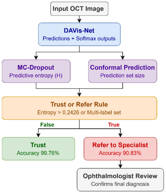
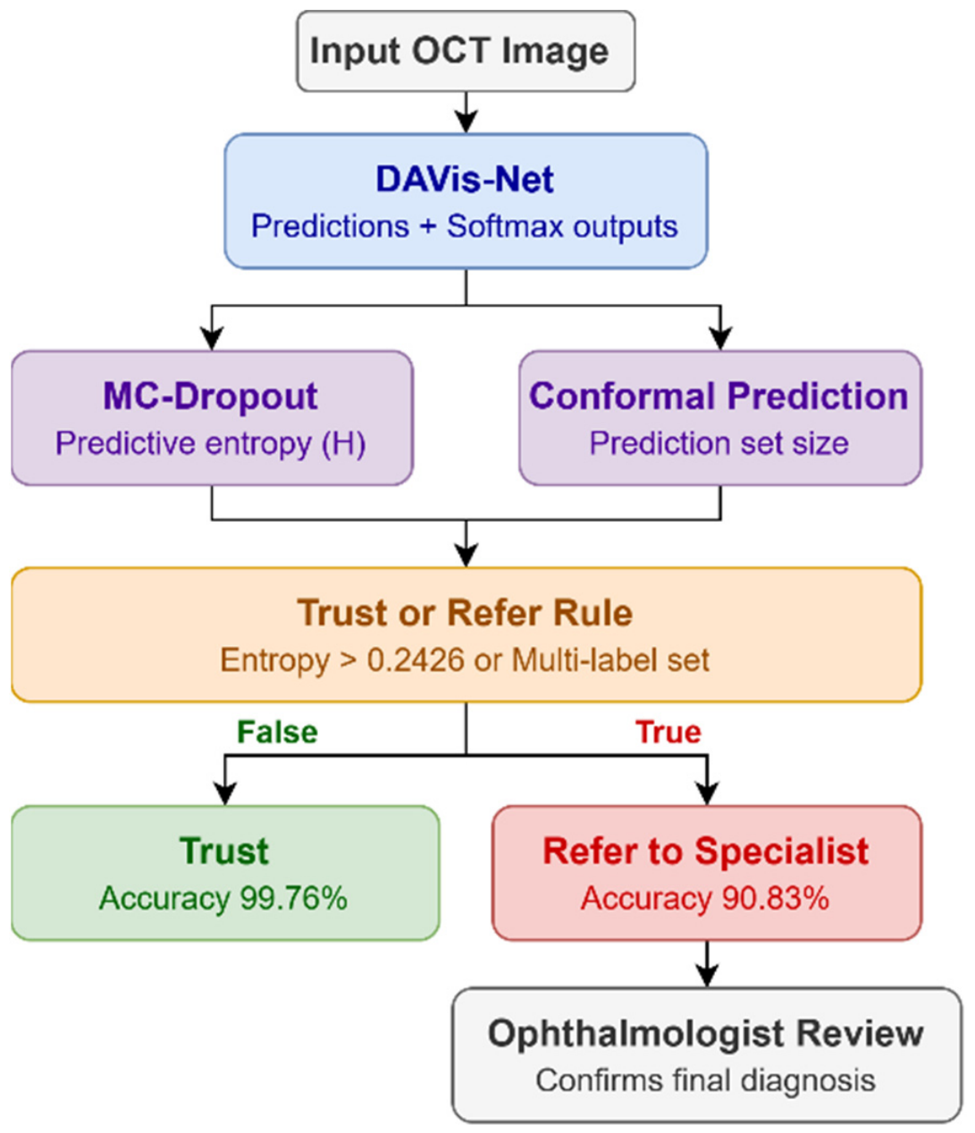
Prediction sets were built at four target coverage levels (90%, 95%, 97%, and 99%) to investigate the relationship between the coverage guarantee and the size of the prediction sets. We then performed a joint reliability analysis to determine whether the three reliability signals (predictive entropy, conformal set size, and Grad-CAM localization score) contain common or class-specific information, using pairwise Pearson correlations within each class. Finally, we built a Trust/Refer triage rule that places a prediction in the Refer bucket if its conformal prediction set has more than one label, or if its predictive entropy exceeds the 75th percentile of predictive entropy for predictions in the calibration split (0.2426). We then calculated accuracy independently in each bucket to see whether the rule was truly triaging.

4. Results

4.1. Overall Classification Performance

Table 6 presents the results of 5-fold cross-validation for both the VGG16 baseline model and DAVis-Net on the same fold splits. DAVis-Net improved the mean accuracy from 97.58% to 98.02%, the mean macro-F1 from 95.91% to 97.35%, and reduced the cross-fold standard deviation on both metrics. The appropriate comparison between the two models is paired, as they were trained and evaluated using exactly identical folds. A paired t-test conducted over the five folds showed an average accuracy increase of +0.44 percentage points. (95% CI [0.10, 0.78], t(4) = 3.59, p = 0.023, Cohen’s $d_z$ = 1.60) and a mean macro-F1 increase of 1.44 percentage points (95% CI [0.78, 2.10], t(4) = 6.08, p = 0.004, $d_z$ = 2.72). This is a small sample for inferential testing, and our DAVis-Net exceeds the baseline in all five folds on both metrics. The direction and consistency of the fold-wise differences and the effect sizes, not the p-value, provide evidence for the conclusion that this improvement is due to the architectural changes, not to the fold level.

Table 6. Fold-wise cross-validation results and paired comparison.

Fold	Accuracy (%)			Macro-F1 Score (%)
	VGG16	DAVis-Net	$\mathbf{\Delta }$ (pp)	VGG16	DAVis-Net	$\mathbf{\Delta }$ (pp)
1	97.67	97.90	+0.23	96.15	97.10	+0.95
2	97.90	98.11	+0.21	96.46	97.41	+0.95
3	97.45	97.98	+0.53	95.62	97.56	+1.94
4	97.31	98.18	+0.87	95.39	97.45	+2.06
5	97.58	97.93	+0.35	95.92	97.24	+1.32
Mean ± SD	97.58 ± 0.22	98.02 ± 0.12	+0.44 ± 0.27	95.91 ± 0.42	97.35 ± 0.18	+1.44 ± 0.53
95% CI			[0.10, 0.78]			[0.78, 2.10]
Cohen’s $d_z$			1.60			2.72
p-value (paired t-test)			0.023			0.004

The improvement was very much class-specific. Averaged across the five folds, DRUSEN F1 improved significantly by 4.57 percentage points (90.55% to 95.12%) when compared with 1.17 points for DME (96.22% to 97.39%) and 0.28 points for CNV (98.66% to 98.94%); NORMAL F1 declined marginally by 0.24 points (98.19% to 97.95%). This is in line with the design objective of DAVis-Net, which uses the two CBAM attention branches to focus on the most important mid-level spatial features for the hardest class, and the auxiliary deep-supervision head to pay attention to the other features. This small drop on NORMAL is consistent with the loss reweighting and the DRUSEN oversampling to move a small amount of decision-boundary capacity away from the easiest class, but is still a reasonable trade-off given the more serious clinical impact of missed pathology.

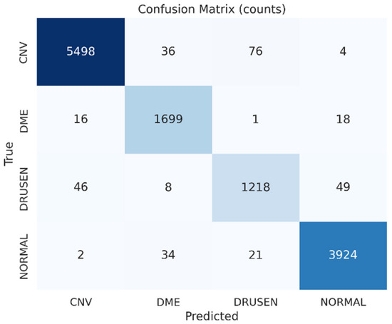
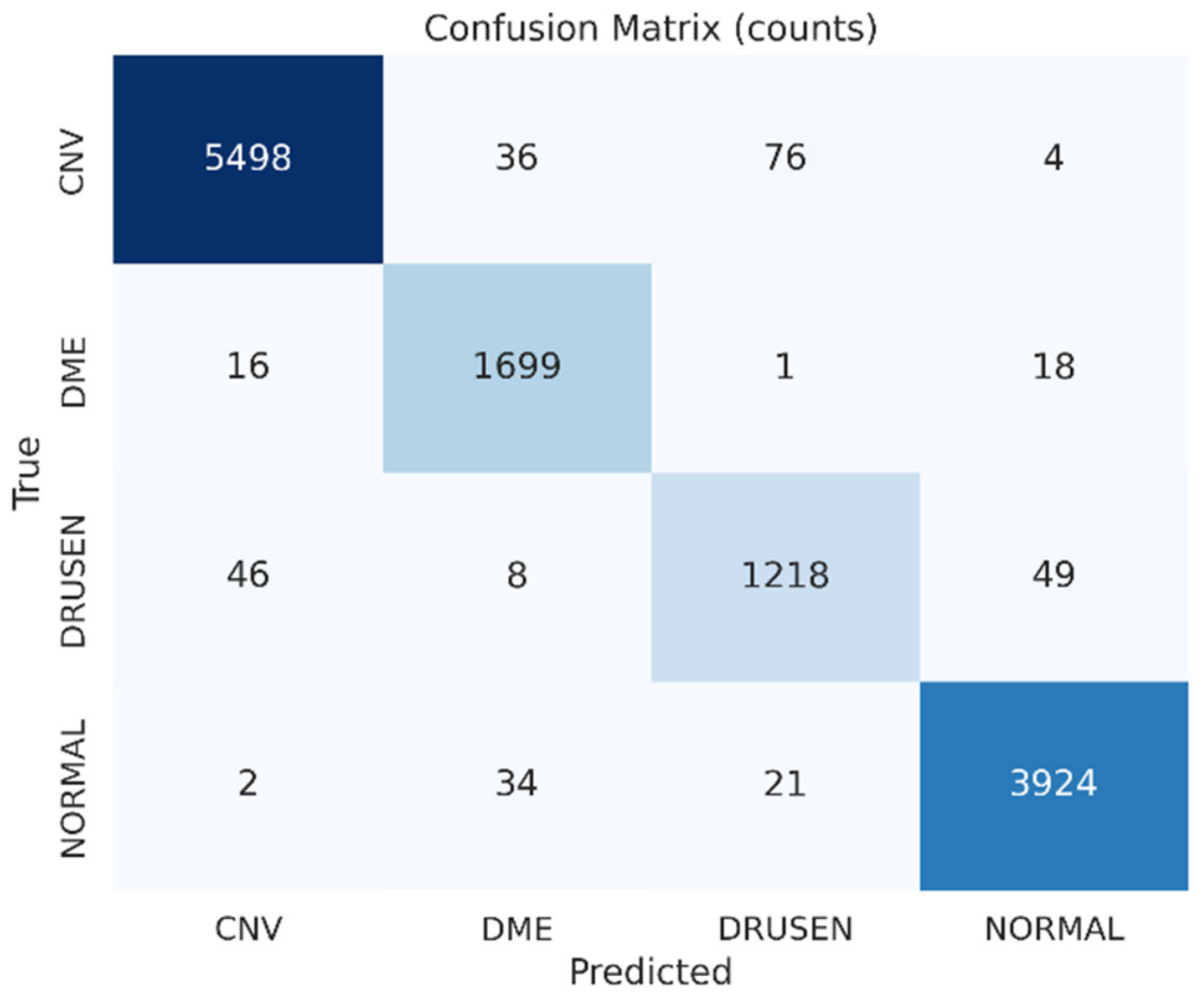
All remaining analyses (Section 4.3, Section 4.4, Section 4.5, Section 4.6 and Section 4.7) were conducted using a single DAVis-Net instance trained on the original training partition, with the original validation partition used for early-stopping monitoring, and evaluated on the held-out test partition, as described in Section 3.4. This model achieved a test accuracy of 97.54%. The confusion matrix and all subsequent reliability assessments were based on this model. Figure 2 shows the confusion matrix on the test set. The matrix shows good overall separation, with a high percentage of samples correctly classified. The residual errors cluster in the DRUSEN row, with 46 cases misclassified as CNV and 49 cases misclassified as NORMAL, resulting in an almost equal distribution between the two classes. This balance is instructive in itself: the plain VGG16 baseline made most of its DRUSEN mistakes as CNV, while DAVis-Net made more evenly distributed mistakes between CNV and NORMAL, indicating that the added attention redistributes the feature emphasis of the model. Clinically, the low error counts for CNV and DME are reassuring, as they are sight-threatening; the residual uncertainty is more likely to be associated with the earlier-stage DRUSEN findings, where a delayed decision is less immediately consequential.

Figure 2. Confusion matrix of DAVis-Net on the test set (n = 12,650).

4.2. Comparison with Existing Methods

Table 7 compares DAVis-Net to some representative classification studies in the literature. DAVis-Net’s cross-validated accuracy of 98.02% is competitive in the field. It clearly outperforms the VGG16 transfer learning method of Jaimes et al. [7] (95.19%) on retinal OCT and is competitive with the ResNet-50 of Akula et al. [8] (97.83%) on retinal OCT. He et al.’s [14] and Li et al.’s [15] transformer models show higher scores, while Ai et al.’s [12] fusion network achieved 98.5% internally but only 81% on external validation. DAVis-Net attains competitive accuracy while additionally providing calibrated, uncertainty-aware, and explainable reliability analysis that none of the compared studies offer.

Table 7. Comparison with existing OCT classification studies.

Study	Model	Accuracy (%)
Kermany et al. [5]	Inception V3	96.60
Jaimes et al. [7]	Modified VGG16	95.19
Akula et al. [8]	ResNet-50	97.83
Huang et al. [11]	Xception + GAB	99.00
Ai et al. [12]	Fusion + CBAM	98.50
He et al. [14]	Swin-Poly	99.80
Li et al. [15]	Swin Transformer V2	99.90
Borah and Singh [29]	ResNet34 + EffNetB4	91.17
DAVis-Net (Ours)	VGG16 + CBAM + DS	98.02 ± 0.12

Computational complexity figures are not included as they were not reported in the original publications, and figures obtained on different hardware would not be comparable.

4.3. Explainability

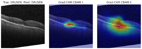
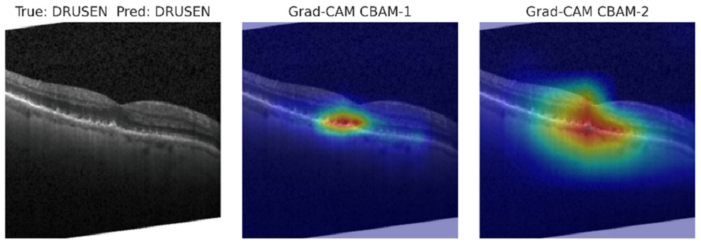
Figure 3 displays the Grad-CAM heatmaps for a correctly classified case, including the original OCT B-scan and the heatmaps generated at both the CBAM-1 and CBAM-2 layers. The two attention scales are complementary and consistent with their location in the network. The CBAM-1 heatmaps, based on the higher-resolution Block 4 features, generate a small, well-defined hot area that is directly above the localized retinal elevation (which is the location of the DRUSEN deposit). The CBAM-2 heat maps, created from deeper layers of Block 5, covered a wider range of the retinal band but remained focused on the same lesion. This validates that the dual placement works as intended: the mid-level module maintains the fine spatial detail of the small deposit, and the deep module extracts the surrounding contextual structure.

Figure 3. An example OCT B-Scan and its corresponding Grad-CAM heatmaps at CBAM-1 and CBAM-2 layers.

Table 8 summarizes the quantitative attribution results, averaged over all classes. The three methods yield similar results across all metrics, with pooled confidence drop ranging from 49.89 to 50.12 and average drop ranging from 54.39 to 54.78 across all methods; for DAVis-Net’s CBAM-refined feature maps, the results suggest that the attribution method has minimal impact on measured faithfulness. Notably, the theoretical improvement that Score-CAM can offer on unstructured backbones does not reflect in the margin, and the authors interpret this as CBAM’s own feature refinement already regularizing the activation maps on which the attribution methods operate. The DRUSEN class shows a distinct drop in confidence and a larger average drop than the other classes. This is because the model becomes ambiguous when the top-attributed region is removed. We confirmed a statistically significant difference between attention quality and correctness by performing a Mann–Whitney U test on the localization score between correctly and incorrectly classified cases (p = 0.0001).

Table 8. Quantitative XAI summary (CBAM-2 Layer, pooled across all classes).

Method	Confidence Drop Top-20% (pp)	Average Drop (%)	Increase-Conf (%)	Cosine Similarity
Grad-CAM	50.06	54.78	3.0	0.716
Grad-CAM++	49.89	54.39	3.0	0.729
Score-CAM	50.12	54.71	2.5	0.711

4.4. Uncertainty and Model Calibration

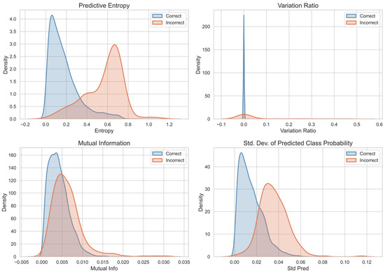
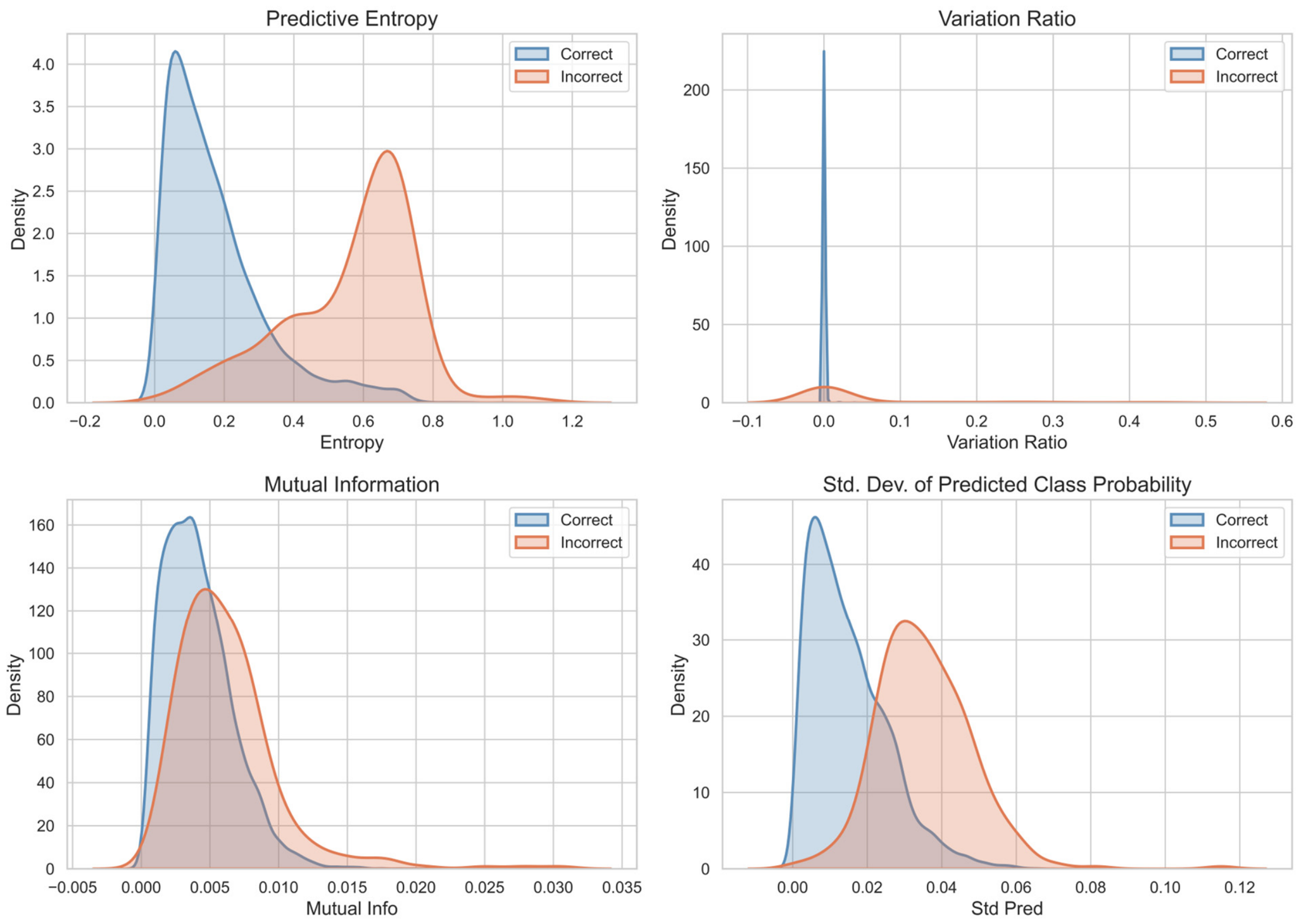
Figure 4 presents the distributions of uncertainty measures by prediction correctness. The distributions in the panels are clean and clinically desirable, with correct predictions tightly grouped around 0 and incorrect predictions forming a second mode around 0.6; high-entropy predictions are much more likely to be incorrect. Variation ratio, mutual information, and standard deviation of the predicted class show the same separation direction but are more similar, so we use entropy as the main uncertainty indicator in the downstream triage rule. Overall, mean entropy for correct predictions is 0.1753 and mean confidence is 0.9522, while for incorrect predictions it is 0.5626 and 0.7286, respectively; both differences are highly significant (Mann–Whitney U, p < 0.001). In practice, model uncertainty can flag a significant proportion of errors before they reach a clinician. This uncertainty is not distributed equally across classes: DRUSEN has a mean entropy of approximately 0.37, between 1.7 and 3 times that of CNV (0.13), DME (0.12), and NORMAL (0.22). The model is therefore not only less accurate for DRUSEN, but also less confident in its predictions, which is exactly what’s needed for safe selective prediction.

Figure 4. Distributions of uncertainty measures.

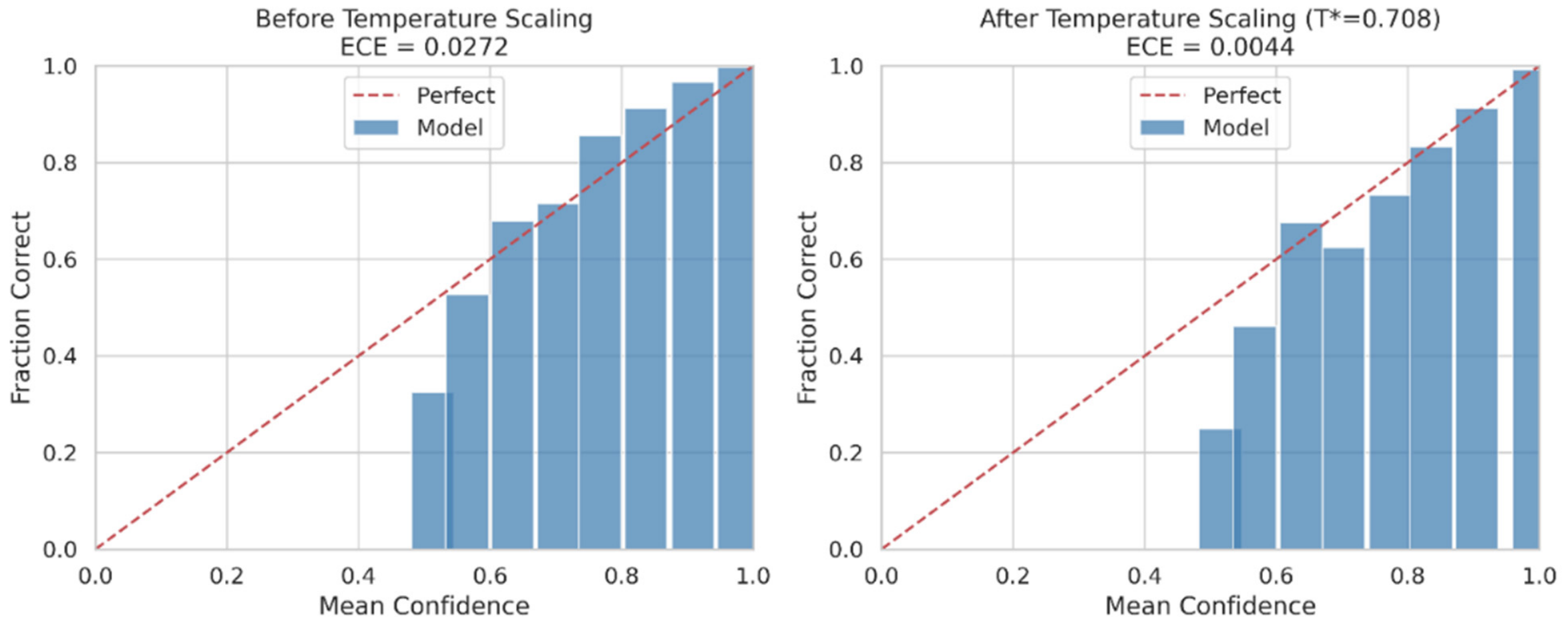
Figure 5 presents the reliability diagram both before and after applying temperature scaling, demonstrating its effect on probability calibration. The reliability curve is consistently below the diagonal in high-confidence bins, the visual signature of overconfidence: if the model reported 90% confidence in that bin, its actual accuracy was slightly lower. Once a single temperature ($T^{\ast }$ = 0.708) is fitted to the validation set, the bars are very close to the diagonal across the entire range of the bars, and the aggregate ECE is reduced from 0.0272 to 0.0044.

Figure 5. Reliability diagram before and after temperature scaling.

Table 9 presents the pre- and post-temperature scaling calibration metrics. Following calibration, the discrepancy between the reported confidence levels and the actual accuracy, measured by Expected calibration error (ECE) and Maximum calibration error (MCE), has significantly reduced by 83.8% and 41.9%, respectively. The Brier score and negative log-likelihood (NLL) have improved modestly by 5.1% and 14.2%, respectively. These metrics evaluate overall probabilistic prediction quality and provide information beyond calibration error alone. Clinically, this step lets us interpret the reported confidence values as close to true-class probabilities, a prerequisite for any subsequent step that relies on probability, such as the conformal prediction and triage analyses that follow.

Table 9. Calibration metrics before and after temperature scaling.

Metric	Before	After	Reduction (%)
ECE	0.0272	0.0044	83.8
MCE	0.4561	0.2650	41.9
Brier Score	0.0395	0.0375	5.1
NLL	0.0909	0.0780	14.2

4.5. Conformal Prediction Results

Table 10 reports the conformal prediction sweep over the four target coverage levels. At 90% and 95%, the empirical coverage aligns with the target, while at 97%, it is 96.68%. The conformal threshold is small, and no prediction set contains more than one class, providing no diagnostic clues about which cases might be confusing the model. We therefore chose the 99% target as the operating point of interest: of the 5062 evaluation samples, 293 were assigned to multi-label prediction sets (5.79%), and the empirical coverage rate (99.23%) was well within the nominal coverage rate, confirming the correctness of the calibration procedure. We note that this coverage guarantee applies to the exchangeability assumption relative to the calibration set, which is sampled from the same single dataset, and not to data from other scanners, sites, or patient populations not included in this dataset. A multi-label set at this level is clinically relevant since it corresponds to a case for which the model, under a strict reliability guarantee, is not ready to make a diagnosis.

Table 10. Conformal prediction across coverage targets.

Target Coverage $(1-\mathit{\alpha })$	Conformal Threshold $\widehat{\mathit{q}}$	Empirical Coverage	Mean Set Size	Multi-Label Sets
90%	0.0568	90.04%	0.906	0
95%	0.1718	95.02%	0.960	0
97%	0.3384	96.68%	0.986	0
99%	0.8808	99.23%	1.058	293

$\widehat{q}$ is the empirical conformal threshold from Equation (10). A class is admitted to the prediction set when the scaled probability is at least $(1-\widehat{q})$.

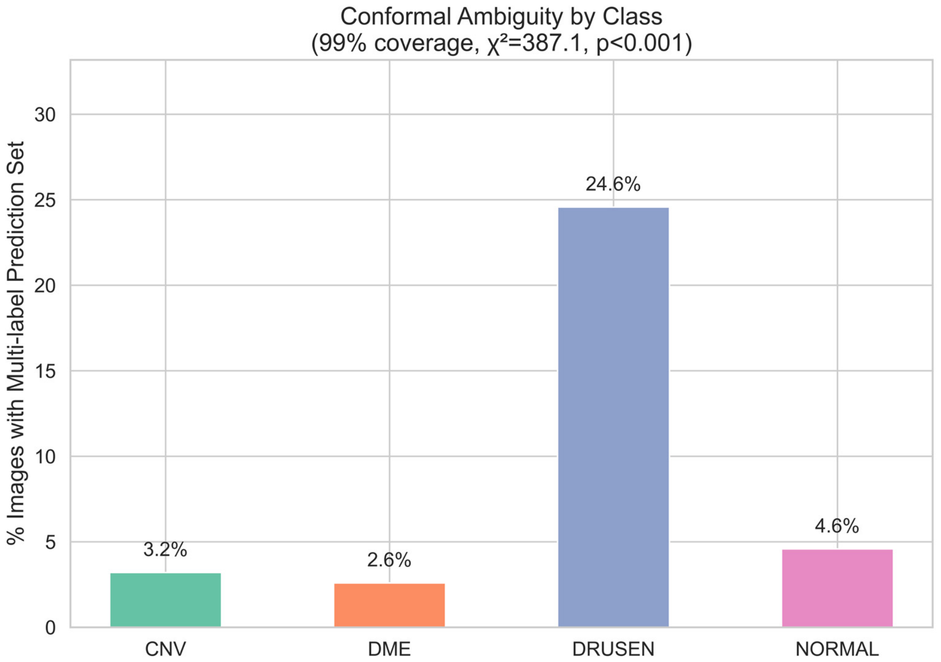
This conformal ambiguity by class is shown in Figure 6. The bar chart is highly skewed, with 24.6% of DRUSEN cases predicted as multi-label, 3.2% of CNV cases, 2.6% of DME cases, and 4.6% of NORMAL cases. This difference is not due to chance, as confirmed by a chi-square test (${\chi }^2$ = 387.1, p < 0.001). The beauty of this result is that it is a probabilistic approach (without ever looking at the confusion matrix or the entropy values); it reaches the same conclusion as these analyses: that the class on which the model is least confident is DRUSEN.

Figure 6. Conformal ambiguity by class.

The error structure of the confusion matrix is reproduced when the composition of ambiguous DRUSEN sets is analyzed, with the majority of cases (84) being DRUSEN combined with CNV, followed by DRUSEN combined with NORMAL (43 cases) and only smaller numbers of {DME, NORMAL} (two cases) and {DME, DRUSEN} (one case), accounting for all 130 multi-label DRUSEN sets. This cross-validation of methods provides evidence of the robustness of the identified ambiguity as a property of the pathology itself, and not a consequence of any single analysis. Table 11 summarizes the pairing counts.

Table 11. Conformal pairing summary.

Prediction Set Pairing	Count
(CNV, DRUSEN)	84
(DRUSEN, NORMAL)	43
(DME, NORMAL)	2
(DME, DRUSEN)	1

4.6. Joint Correlation Analysis

The pairwise Pearson correlations between the three reliability signals across the four classes show two clearly discernible patterns that do not differ between classes. First, the size of the conformal sets is highly positively correlated with entropy, with correlation coefficients of 0.69 for CNV, 0.67 for DME, 0.78 for DRUSEN, and 0.69 for NORMAL. Both essentially measure the same fundamental property of the model—its sharpness, or the sharpness of its predictive distribution—and are largely synonymous. Second, entropy and set size do not correlate with the localization score, with coefficients ranging from −0.07 to +0.01 in each class. Table 12 summarizes the per-class numbers.

Table 12. Per-class Pearson correlations between reliability signals.

Class	Entropy to Set Size	Entropy to Localization	Set Size to Localization
CNV	0.69	0.01	−0.01
DME	0.67	−0.07	−0.03
DRUSEN	0.78	−0.06	−0.01
NORMAL	0.69	−0.07	−0.03

Correlations were computed on the conformal evaluation split (n = 5062: CNV 2246; DME 694; DRUSEN 529; NORMAL 1593).

The primary methodological insight derived from this study pertains to the localization proxy: both entropy and conformal set size exhibit a near-zero linear (Pearson) correlation with the localization score. This contrasts sharply with the strong mutual correlation between entropy and conformal set size themselves (r = 0.67–0.78). This near-zero correlation, specific to this proxy and the linear correlation method used, does not preclude a nonlinear relationship or one that could be identified through a more direct, expert-validated localization measure. A model may confidently predict even when attention is directed outside the central macular region or display high uncertainty despite accurate attention placement. These two families of signals encapsulate different aspects of model behavior and serve as complementary indicators. This finding highlights the importance of tracking both the distributional and spatial signals in a deployed system. However, since the localization measure is still a geometric proxy without lesion-level validation, only the two distributional signals—entropy and conformal set size—currently influence the Trust/Refer decision rule.

4.7. Trust/Refer Triage

The composite Trust/Refer rule transforms the reliability signals into a decision. Figure 7, “Trust/Refer Triage Rule Workflow,” illustrates the logic for routing an incoming prediction to the Refer bucket when the conformal set is multi-label or when its predictive entropy exceeds the 75th percentile threshold (0.2426) derived from the calibration, and to the Trust bucket otherwise.

Figure 7. Trust/Refer Triage Rule Workflow.

Table 13 reports the rule’s performance. The Trust bucket has 73.9% of the evaluation samples and 99.76% accuracy, whereas the Refer bucket has 26.1% of the evaluation samples and 90.83% accuracy. The 8.93-point difference suggests the rule is not cutting the data randomly; it is focusing the model’s residual errors on the minority of cases it flags for human review. This would enable about 75% of scans to be dealt with close to perfectly, and specialist resources to be focused on the quarter of cases that needed them the most. We emphasize that this is a retrospective, internal, image-level result on a single held-out evaluation subset and does not constitute a validated clinical workflow (Section 5.4). As with all previous analyses, DRUSEN (72.4%) had the highest referral rate, and much lower referral rates for NORMAL (34.5%), CNV (13.7%), and DME (11.7%), which means that the class on which the model is most ambiguous is the most frequently referred class for specialist review, which is precisely how any triage rule should operate. Table 14 summarizes performance by class.

Table 13. Trust/Refer triage performance.

Bucket	N	Proportion (%)	Accuracy (%)	Errors (n)
Trust	3742	73.9	99.76	9
Refer	1320	26.1	90.83	121

Table 14. Class-specific retention and referral rates of the Trust/Refer rule.

Class	N	Trust			Refer
		N	% of Class	Accuracy (%)	N	% of Class	Accuracy (%)
CNV	2246	1939	86.3	99.85	307	13.7	86.64
DME	694	613	88.3	100.00	81	11.7	88.89
DRUSEN	529	146	27.6	97.26	383	72.4	90.60
NORMAL	1593	1044	65.5	99.81	549	34.5	93.62
Pooled	5062	3742	73.9	99.76	1320	26.1	90.83

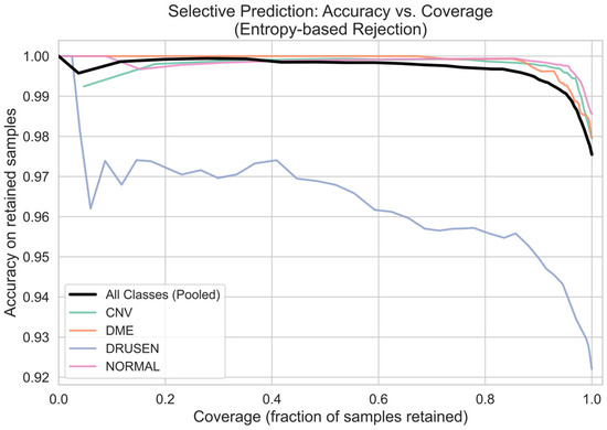
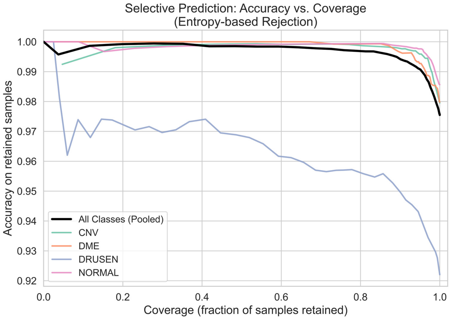
Figure 8 further supports the generality of the underlying entropy signal by showing the accuracy of retained predictions as more high-entropy samples are rejected. The pooled curve is smooth and monotonically increasing as coverage drops, validating that entropy-based rejection is valid not only at the class level but also for the model as a whole. The per-class curves are all increasing at every operating point, and the DRUSEN curve is consistently below the rest of the curves over the entire coverage range, reaffirming the observation that DRUSEN is the most difficult class at all operating points, yet still enjoys selective rejection. This shows that the triage mechanism is a general-purpose reliability tool, not a DRUSEN-specific patch.

Figure 8. Selective prediction: Accuracy vs. Coverage.

5. Discussion

5.1. Principal Findings

The main objective of this study was to determine whether a medical image classifier is better described by the interaction of reliability signals than by accuracy alone. The results of the study support the hypothesis; DAVis-Net achieved a statistically significant improvement over the VGG16 baseline (98.02% vs. 97.58% accuracy, p = 0.023; 97.35% vs. 95.91% macro-F1, p = 0.004), with lower cross-fold variance and the improvement focused on the hardest class. This selective behavior is consistent with the architectural hypothesis: a second CBAM module keeps the mid-level spatial attention, while providing direct gradient supervision to mid-level features is sufficient to deal with the specific representational disadvantage of small, focal, low-contrast pathology, without interfering with the features that work well for the well-separated classes.

The most important finding, however, is not the gain in accuracy but the structure shown by the joint correlation analysis. The predictive entropy and the size of the conformal sets were found to be highly correlated across all four classes, whereas the quality of the attribution localization was orthogonal. This indicates that, according to our central-region localization proxy, distributional uncertainty and the placement of explanations for spatial model behavior are likely distinct aspects of model behavior, not the same. A model can be confident but misdirected, or unsure but properly focused. The practical corollary is that a trustworthy decision-support system should monitor both, as each can detect failures the other misses; relying on uncertainty alone would miss confident but spatially misdirected predictions, and relying on explanation alone would miss well-localized (but uncertain) ones. The Trust/Refer rule demonstrates an accuracy disparity of nearly nine percentage points between its two categories, based on a retrospective analysis conducted within our internal evaluation subset (Section 4.7). Notably, this rule integrates two distributional criteria—conformal set size and predictive entropy—and intentionally omits the localization proxy; the near-zero correlation suggests that an authenticated spatial signal might provide information beyond these two distributional criteria. However, confirming this hypothesis and establishing a spatial criterion for application in a clinical decision-making context would necessitate lesion-level ground truth data, which was not available in this instance.

5.2. Positioning Relative to the Existing Work

DAVis-Net’s 98.02% cross-validated accuracy exceeds the 95.19% reported by Jaimes et al. [7] for a modified VGG16 under 10-fold Monte Carlo cross-validation, and modestly exceeds the 97.83% of Akula et al. [8] for ResNet-50. The latter is the comparison least favorable to us: Akula et al. used a stratified patient-level split, whereas our figure is obtained on an image-level split, so the two numbers are not measuring the same quantity. Transformer-based studies report higher accuracies still—99.80% for the Swin-Poly network of He et al. [14] and 99.90% for the Swin Transformer V2 of Li et al. [15]—and we do not claim to match them. The fusion network of Ai et al. [12] reports 98.50% internally, which does not differ meaningfully from our result, but falls to 81–92% on external validation.

Where the present study differs is in what it reports beyond accuracy. The transformer studies [14,15,16] present attribution maps but assess them qualitatively rather than testing faithfulness. The attribution-evaluation studies [21,22] quantify faithfulness rigorously but do not relate it to predictive uncertainty. The conformal studies [27,28,29] report coverage and set size but do not analyze attribution. The consequence is that the central empirical question of this paper—whether uncertainty and explanation signals carry overlapping or independent information—could not have been answered from the existing literature, because no prior study reports both quantities for the same predictions.

Our results also reinforce that the DRUSEN-associated class is the weakest class in Kermany et al. [5], Jaimes et al. [7], and Novely et al. [10], across different architectures, dataset versions, and class taxonomies. It is the weakest class here across five methodologically independent measurements: per-class F1 (95.12% against 97.39–98.94% for the other classes), class-conditional predictive entropy (0.372 against 0.122–0.223), conformal ambiguity rate (24.57% against 2.59–4.58%), triage referral rate (72.4% against 11.7–34.5%), and the selective-prediction curve, on which DRUSEN lies below the other three classes at every operating point. This difficulty reflects the pathology, whose sub-RPE morphology overlaps with both incipient neovascular change and normal retinal aging [2,3], rather than any particular model.

5.3. Clinical Relevance

The clinical usefulness of the framework is not in its absolute level of accuracy but in revealing and dealing with uncertainty. The temperature-scaling result is a prerequisite for all downstream activities: the model’s stated confidence, which is 90%, is numerically trustworthy, meaning that after calibration, the predicted confidence is substantially better aligned with empirical accuracy, such that predictions assigned approximately 90% confidence exhibit approximately 90% empirical accuracy in the corresponding calibration regime. A clinician, or an automated rule, can make a reasonable decision based on the probabilities only after they have been calibrated like this. It follows that the Trust/Refer triage would correspond to a workflow in which approximately three-quarters of scans are automatically processed with 99.76% accuracy, and the remaining quarter (which contains most of the model’s errors) is referred to a specialist for further review. This describes a retrospective internal discovery rather than a clinically validated workflow; further prospective evaluation, as discussed in Section 5.5, is necessary before such a workflow could be deployed. This uncertainty-aware, risk-based approach is consistent with the direction that Kurz et al. [25] proposed for the field, as well as with the risk-based routing that Angelopoulos and Bates [26] identified as a natural application of conformal prediction in healthcare.

A second clinically relevant finding is the converging evidence on the DRUSEN class. The confusion matrix, the class-wise entropy, the calibration error, the conformal ambiguity rate, and the attribution concentration all show that the model is the least confident on the DRUSEN class. Fortunately, the model’s errors are concentrated in this earlier-stage finding, not in the more pressing, sight-threatening CNV and DME categories, where residual error was small. The convergence itself has operational value: a screening system could preemptively route scans of patients suspected of having DRUSEN for human confirmation, even if the reported confidence were low, because early DRUSEN can have morphology similar to both incipient neovascular change and normal retinal aging [2,3]. The uncertainty behavior of the framework is consistent with the clinical intuition in this sense.

5.4. Limitations

The publicly available dataset partition is organized at the image level rather than the patient level, which could lead to data leakage since B-scans from the same patient might appear in multiple partitions. All reported metrics—accuracy, calibration, conformal coverage and triage performance—are therefore internal, image-level estimates and should not be interpreted as estimates of patient-independent generalization. The literature provides direct evidence that this distinction matters: FN-OCT [12] dropped from 98.5% to 81% on external validation, and GABNet [11] from 99% to 91.41%. Furthermore, the calibration and conformal guarantees are themselves distribution-dependent; transfer to a new scanner or clinical site would require re-calibration on local data. The transformer-based models in Table 7 report higher headline accuracy, but none report calibration, uncertainty, or conformal analysis, so whether the reliability structure identified here extends beyond CNN-based classifiers remains an open question that we identify as a direct extension of this work.

The localization score used in the joint correlation analysis is a geometric proxy—the fraction of Grad-CAM energy in the central 25% of the image area—not a measure of agreement with clinician-delineated lesion boundaries, which were unavailable for this dataset. This proxy is poorly matched to spatially diffuse pathology such as intraretinal cystoid spaces in DME or peripheral DRUSEN, and the resulting measurement noise would tend to attenuate any true correlation, so the near-zero values in Table 12 should be read as lower bounds rather than proof of absence. We note that the perturbation-based faithfulness metrics (confidence drop, average drop) do not depend on lesion annotations and are unaffected by this limitation.

Finally, we conducted the reliability analyses in Section 4.3, Section 4.4, Section 4.5, Section 4.6 and Section 4.7 on a single separately trained model (97.54% test accuracy) rather than across the five cross-validation folds, and we evaluated the Trust/Refer triage rule retrospectively rather than through a prospective reader study with clinicians. Both would strengthen the evidence but were beyond the scope and resources of this study.

5.5. Future Scope

The first priority is re-evaluation under a strict patient-level partition to determine whether the reported performance and the reliability structure persist once patient-specific appearance cues are removed. Multi-center and cross-scanner validation is the second priority, as all current results are internal to a single dataset and scanner.

The localization proxy should be replaced with expert-delineated lesion segmentations, which would convert the spatial component of the reliability analysis from a geometric approximation to a clinically grounded measure. We can test whether the near-zero correlation we observed between distributional uncertainty and the spatial localization proxy generalizes by varying three factors: pathology scale (focal vs. diffuse), architecture family (CNN vs. transformer), and the localization measure itself. Reproducing a transformer backbone under the full reliability pipeline would additionally address the accuracy comparison gap identified in this study.

Last, prospective evaluation of the Trust/Refer workflow in a clinical decision-support setting, including a reader study with practicing ophthalmologists, would provide the real-world evidence of utility that retrospective analysis cannot.

6. Conclusions

This study introduced the DAVis-Net architecture, based on the VGG16 network and supplemented with dual CBAM attention and an auxiliary deep-supervision head, along with a comprehensive reliability evaluation framework for four-class retinal OCT classification. The framework achieved a 5-fold cross-validated accuracy of 98.02%, significantly outperforming the VGG16 baseline (accuracy p = 0.023; macro-F1 p = 0.004). These improvements mainly targeted the most difficult class (DRUSEN), with only slight, previously noted trade-offs in the simplest class (NORMAL; Section 4.1). The integrated reliability analysis includes MC Dropout uncertainty estimation, temperature scaling calibration (which reduced ECE from 0.0272 to 0.0044), and split conformal prediction (with 99.23% empirical coverage at a mean set size of 1.058). Quantitative multi-method explainability demonstrated that predictive entropy and conformal set size were highly correlated signals, indicating redundancy. Meanwhile, their near-zero linear correlation with attribution localization—assessed through our central-region proxy—implies that these metrics may represent largely distinct facets of model behavior, specific to the proxy employed in this analysis. A composite Trust/Refer rule combining predictive entropy with conformal set size divided the evaluation set into a high-reliability majority (73.9% of cases), classified at 99.76% accuracy, and a low-reliability minority set routed for specialist review (26.1% of cases), with 90.83% accuracy. These results collectively show that multi-dimensional reliability characterization is a more clinically relevant method for evaluating a medical image classifier than accuracy, and provide a roadmap towards trustworthy OCT-based decision support. We emphasize that all figures reported are internal estimates obtained on a single dataset under an image-level partition, and that patient-level re-partitioning, multi-center validation, and prospective clinical evaluation are prerequisites for any clinical claim.

References

- Zeppieri, M.; Marsili, S.; Enaholo, E.S.; Shuaibu, A.O.; Uwagboe, N.; Salati, C.; Spadea, L.; Musa, M. Optical Coherence Tomography (OCT): A Brief Look at the Uses and Technological Evolution of Ophthalmology. Medicina 2023, 59, 2114. [Google Scholar] [CrossRef] [Scilit] [PubMed]
- Iliescu, D.A.; Ghita, A.C.; Ilie, L.A.; Voiculescu, S.E.; Geamanu, A.; Ghita, A.M. Non-Neovascular Age-Related Macular Degeneration Assessment: Focus on Optical Coherence Tomography Biomarkers. Diagnostics 2024, 14, 764. [Google Scholar] [CrossRef] [Scilit] [PubMed]
- Gorbatova, A. OCT Biomarkers in Age-Related Macular Degeneration. Bachelor’s Thesis, Oulu University of Applied Sciences, Oulu, Finland, 2025. [Google Scholar]
- Schmidt-Erfurth, U.; Sadeghipour, A.; Gerendas, B.S.; Waldstein, S.M.; Bogunović, H. Artificial Intelligence in Retina. Prog. Retin. Eye Res. 2018, 67, 1–29. [Google Scholar] [CrossRef] [Scilit] [PubMed]
- Kermany, D.S.; Goldbaum, M.; Cai, W.; Valentim, C.C.S.; Liang, H.; Baxter, S.L.; McKeown, A.; Yang, G.; Wu, X.; Yan, F.; et al. Identifying Medical Diagnoses and Treatable Diseases by Image-Based Deep Learning. Cell 2018, 172, 1122–1131.e9. [Google Scholar] [CrossRef] [Scilit] [PubMed]
- Simonyan, K.; Zisserman, A. Very deep convolutional networks for large-scale image recognition. arXiv 2014, arXiv:1409.1556. [Google Scholar]
- Jaimes, W.J.; Arenas, W.J.; Navarro, H.J.; Altuve, M. Detection of Retinal Diseases from OCT Images Using a VGG16 and Transfer Learning. Discov. Appl. Sci. 2025, 7, 160. [Google Scholar] [CrossRef] [Scilit]
- Akula, K.; Pusuluri, V.B.; Nagendla, P.B. Deep Learning-Based Multi-Class Classification of Retinal Diseases from OCT Images Using Transfer Learning. J. Comput. Commun. 2026, 14, 220–230. [Google Scholar] [CrossRef] [Scilit]
- Woo, S.; Park, J.; Lee, J.-Y.; Kweon, I.S. CBAM: Convolutional block attention module. In Proceedings of the European Conference on Computer Vision (ECCV); Springer: Cham, Switzerland, 2018; pp. 3–19. [Google Scholar]
- Novely, N.; Mahmud Shuvo, S.; Faruk, M.F. Improving Pre-Trained CNNs with CBAM and Skip Connections for Multi-Class Retinal Diseases Classification Using OCT Images. In Proceedings of the 3rd International Conference on Computing Advancements; ACM: Dhaka, Bangladesh, 2024; pp. 946–953. [Google Scholar]
- Huang, X.; Ai, Z.; Wang, H.; She, C.; Feng, J.; Wei, Q.; Hao, B.; Tao, Y.; Lu, Y.; Zeng, F. GABNet: Global Attention Block for Retinal OCT Disease Classification. Front. Neurosci. 2023, 17, 1143422. [Google Scholar] [CrossRef] [Scilit] [PubMed]
- Ai, Z.; Huang, X.; Feng, J.; Wang, H.; Tao, Y.; Zeng, F.; Lu, Y. FN-OCT: Disease Detection Algorithm for Retinal Optical Coherence Tomography Based on a Fusion Network. Front. Neuroinform. 2022, 16, 876927. [Google Scholar] [CrossRef] [Scilit] [PubMed]
- Fang, L.; Wang, C.; Li, S.; Rabbani, H.; Chen, X.; Liu, Z. Attention to Lesion: Lesion-Aware Convolutional Neural Network for Retinal Optical Coherence Tomography Image Classification. IEEE Trans. Med. Imaging 2019, 38, 1959–1970. [Google Scholar] [CrossRef] [Scilit] [PubMed]
- He, J.; Wang, J.; Han, Z.; Ma, J.; Wang, C.; Qi, M. An Interpretable Transformer Network for Retinal Disease Classification Using Optical Coherence Tomography. Sci. Rep. 2023, 13, 3637. [Google Scholar] [CrossRef] [Scilit] [PubMed]
- Li, Z.; Han, Y.; Yang, X. Multi-Fundus Diseases Classification Using Retinal Optical Coherence Tomography Images with Swin Transformer V2. J. Imaging 2023, 9, 203. [Google Scholar] [CrossRef] [Scilit] [PubMed]
- Upmanu, V.; Singh, J.; Saxena, P.; Singh, J.; Srivast, S.; Tripathi, A. A Novel Clinically Explainable Vision Transformer for OCT-Based Retinal Disease Classification: Integrating UniMIE Enhancement and Grad-CAM Interpretability. Res. Sq. 2025. [Google Scholar] [CrossRef] [Scilit] [PubMed]
- Faghani, S.; Moassefi, M.; Rouzrokh, P.; Khosravi, B.; Baffour, F.I.; Ringler, M.D.; Erickson, B.J. Quantifying Uncertainty in Deep Learning of Radiologic Images. Radiology 2023, 308, e222217. [Google Scholar] [CrossRef] [Scilit] [PubMed]
- Selvaraju, R.R.; Cogswell, M.; Das, A.; Vedantam, R.; Parikh, D.; Batra, D. Grad-CAM: Visual Explanations from Deep Networks via Gradient-Based Localization. In Proceedings of the IEEE International Conference on Computer Vision (ICCV); IEEE: Piscataway, NJ, USA, 2017; pp. 618–626. [Google Scholar]
- Chattopadhyay, A.; Sarkar, A.; Howlader, P.; Balasubramanian, V.N. Grad-CAM++: Improved Visual Explanations for Deep Convolutional Networks. In Proceedings of the 2018 IEEE Winter Conference on Applications of Computer Vision (WACV); IEEE: Piscataway, NJ, USA, 2018; pp. 839–847. [Google Scholar]
- Wang, H.; Wang, Z.; Du, M.; Yang, F.; Zhang, Z.; Ding, S.; Mardziel, P.; Hu, X. Score-CAM: Score-Weighted Visual Explanations for Convolutional Neural Networks. In Proceedings of the IEEE/CVF Conference on Computer Vision and Pattern Recognition Workshops (CVPRW); IEEE: Piscataway, NJ, USA, 2020; pp. 111–119. [Google Scholar]
- Singh, A.; Balaji, J.J.; Rasheed, M.A.; Jayakumar, V.; Raman, R.; Lakshminarayanan, V. Quantitative and Qualitative Evaluation of Explainable Deep Learning Methods for Ophthalmic Diagnosis. arXiv 2020, arXiv:2009.12648. [Google Scholar]
- Yavari, A.; Schmoll, T.; Leitgeb, R.A.; Huber, K.L.; Stino, H.; Pollreisz, A.; Drexler, W.; Schlegl, T. Applicability Study of AI Attribution Methods for Ophthalmic Image Classification. Sci. Rep. 2026, 16, 3296. [Google Scholar] [CrossRef] [Scilit] [PubMed]
- Rong, Y.; Leemann, T.; Borisov, V.; Kasneci, G.; Kasneci, E. A Consistent and Efficient Evaluation Strategy for Attribution Methods. arXiv 2022, arXiv:2202.00449. [Google Scholar]
- Gal, Y.; Ghahramani, Z. Dropout as a Bayesian Approximation: Representing Model Uncertainty in Deep Learning. In Proceedings of the 33rd International Conference on Machine Learning (ICML); PMLR 48; PMLR: Cambridge, MA, USA, 2016; pp. 1050–1059. [Google Scholar]
- Kurz, A.; Hauser, K.; Mehrtens, H.A.; Krieghoff-Henning, E.; Hekler, A.; Kather, J.N.; Fröhling, S.; Von Kalle, C.; Brinker, T.J. Uncertainty Estimation in Medical Image Classification: Systematic Review. JMIR Med. Inform. 2022, 10, e36427. [Google Scholar] [CrossRef] [Scilit] [PubMed]
- Angelopoulos, A.N.; Bates, S. A Gentle Introduction to Conformal Prediction and Distribution-Free Uncertainty Quantification, Found. Trends Mach. Learn. 2022, 16, 494–591. [Google Scholar]
- Ghoshal, B.; Woof, W.; Mendes, B.; Al-Khuzaei, S.; De Guimaraes, T.A.C.; Varela, M.D.; Liu, Y.; Sen, S.; Lin, S.; Shah, M.; et al. Making Deep Learning Models Clinically Useful—Improving Diagnostic Confidence in Inherited Retinal Disease with Conformal Prediction. In Uncertainty for Safe Utilization of Machine Learning in Medical Imaging; Sudre, C.H., Mehta, R., Ouyang, C., Qin, C., Rakic, M., Wells, W.M., Eds.; Springer Nature: Cham, Switzerland, 2025; Volume 15167, pp. 47–58. [Google Scholar]
- Hirsch, R.; Goldberger, J. A Conformalized Learning of a Prediction Set with Applications to Medical Imaging Classification. In Proceedings of the IEEE International Symposium on Biomedical Imaging (ISBI); IEEE: Piscataway, NJ, USA, 2024; pp. 1–5. [Google Scholar]
- Borah, J.; Singh, H.K. Interpretable Deep Learning Framework for Improved Disease Classification in Medical Imaging. arXiv 2026, arXiv:2503.11851. [Google Scholar]
- He, K.; Zhang, X.; Ren, S.; Sun, J. Deep Residual Learning for Image Recognition. In Proceedings of the IEEE Conference on Computer Vision and Pattern Recognition (CVPR); IEEE: Piscataway, NJ, USA, 2016; pp. 770–778. [Google Scholar]
- Huang, G.; Liu, Z.; van der Maaten, L.; Weinberger, K.Q. Densely Connected Convolutional Networks. In Proceedings of the IEEE Conference on Computer Vision and Pattern Recognition (CVPR); IEEE: Piscataway, NJ, USA, 2017; pp. 4700–4708. [Google Scholar]
- Chollet, F. Xception: Deep Learning with Depthwise Separable Convolutions. In Proceedings of the IEEE Conference on Computer Vision and Pattern Recognition (CVPR); IEEE: Piscataway, NJ, USA, 2017; pp. 1251–1258. [Google Scholar]
- Tan, M.; Le, Q.V. EfficientNet: Rethinking Model Scaling for Convolutional Neural Networks. In Proceedings of the 36th International Conference on Machine Learning (ICML); PMLR: Cambridge, MA, USA, 2019; pp. 6105–6114. [Google Scholar]
Disclaimer/Publisher’s Note: The statements, opinions and data contained in all publications are solely those of the individual author(s) and contributor(s) and not of MDPI and/or the editor(s). MDPI and/or the editor(s) disclaim responsibility for any injury to people or property resulting from any ideas, methods, instructions or products referred to in the content. |
© 2026 by the authors. Licensee MDPI, Basel, Switzerland. This article is an open access article distributed under the terms and conditions of the Creative Commons Attribution (CC BY) license.