Quiescent Optical Solitons for Cubic–Quintic Nonlinear Schrödinger’s Equation with Intensity-Dependent Dispersion and Weak Nonlocality

Abstract

This study examined quiescent optical structures in a cubic–quintic nonlinear Schrödinger model that combines intensity-dependent dispersion with a weakly nonlocal intensity-curvature response. A real phase–amplitude reduction establishes the compatibility conditions for stationary localized profiles. The enhanced direct algebraic method then produces regular bright and dark states, singular hyperbolic states, and Jacobi and Weierstrass elliptic families. Spatially shifted formulas are identified as translated representatives rather than new orbit types. Each family is validated through the auxiliary equation, the stationary residual, explicit reality and nondegeneracy restrictions, and an independent first-integral formulation. The quintic response changes the dominant balance and the admissible coefficient manifolds relative to the corresponding Kerr-only setting. Parameter continuations illustrate distinct roles of cubic, quintic, dispersive, and weakly nonlocal effects without implying unconstrained one-parameter dynamics. For a representative regular bright state, refined Chebyshev collocation locates no persistent unstable eigenvalue and direct Fourier propagation under simultaneous amplitude and phase perturbations remains bounded. The numerical conclusion is restricted to the tested branch and finite propagation interval.

1. Introduction

The nonlinear Schrödinger equation is a central envelope model for the competition between dispersion and self-phase modulation in optical media. Its cubic–quintic extension incorporates a higher-order refractive response that can reinforce, saturate, or oppose the Kerr contribution, thereby changing the existence, shape, and stability of coherent optical structures [1,2,3]. Intensity-dependent dispersion introduces a separate mechanism because the local field intensity changes the coefficient multiplying the envelope curvature. Analytical and variational studies have established stationary, compact, and singular branches in such models [4,5,6], while subsequent work has clarified the interplay with Kerr nonlinearity and the branch-dependent character of stability [7,8,9]. Hence, the existence of an exact profile and one numerical test cannot establish global stability. A recent Kerr-only optical study also used an algebraic construction to obtain quiescent profiles in a related setting [10].

For a broader contemporary optoelectronic context, light-excited carrier transport across GaAs p–n junctions under interband and intraband excitation has also been examined recently [11]; this semiconductor-transport setting is physically distinct from the nonlinear envelope dynamics considered here.

Weak nonlocality is physically distinct from dispersion because the refractive-index response samples a narrow spatial neighborhood rather than only the local intensity. Weakly nonlocal nonlinear Schrödinger models support modified bright, dark, periodic, and singular waves, with altered stability properties [12,13,14]; related work has also reported Jacobi elliptic families and modulational-instability changes [15]. The combined effect of cubic–quintic refraction, intensity-dependent dispersion, and weak nonlocality has received less attention. The closest cubic–quintic weakly nonlocal study omits the intensity-dependent envelope-curvature contribution [14], whereas closely related intensity-dependent-dispersion studies mainly use the Kerr response or different refractive laws [10,16]. Earlier related studies have reported periodic waves for a time-fractional perturbed nonlinear Schrödinger model in optical fibers [17] and optical soliton families supported by sensitivity or stability analyses in other governing equations [18,19]. These studies, however, do not treat the present deterministic cubic–quintic model with simultaneous intensity-dependent envelope curvature and weak nonlocality. Related optical-metamaterial work has also used Lie-symmetry reduction for implicit quiescent soliton perturbations with nonlinear chromatic dispersion and Kudryashov’s quintuple form of self-phase modulation [20].

Related extensions include Lie-symmetry reductions of higher-order Schrödinger–Hirota models with nonlinear dispersive perturbations and proportional vector quiescent states in coupled systems with nonlinear dispersion [21,22]. These studies concern different governing equations and do not include the simultaneous cubic–quintic and weakly nonlocal structure considered here. The present work addresses this intersection using the enhanced direct algebraic method to construct selected regular, singular, hyperbolic, and elliptic stationary families. Algebraic closure is supplemented by direct residual tests, explicit reality and nondegeneracy conditions, a first-integral check, spectral refinement, and direct perturbed propagation; the resulting catalog is not claimed to exhaust all stationary solutions of the model.

The closest model classes and their distinctions from the present formulation are summarized in Table 1.

Table 1. Comparison with the closest model classes used to position the present work.

Study	Governing Nonlinearities	Principal Solution Classes	Validation/Stability Emphasis
Ref. [14]	Cubic–quintic refraction with weak nonlocality; no intensity-dependent dispersion.	Chirped periodic and localized exact waves.	Analytical exact-wave construction; it provides the closest weakly nonlocal cubic–quintic comparator, but not the present combined derivative structure.
Refs. [4,5,6,7,8,9]	Intensity-dependent dispersion with Kerr-type response; no simultaneous weakly nonlocal cubic–quintic combination.	Stationary/localized solitary waves, including smooth and black-soliton branches.	Analytical/variational characterization, with dedicated branch-dependent stability analyses in Refs. [8,9].
Refs. [10,16]	Nonlinear or intensity-dependent dispersion with Kerr or other refractive laws; no simultaneous cubic–quintic weak-nonlocal structure.	Quiescent or stationary exact solitons.	Closed-form/algebraic constructions used as nonlinear-dispersion comparators; stability conclusions are not transferred to the present PDE.
Present work	Cubic–quintic refraction with intensity-dependent dispersion and weak nonlocality.	Regular bright/dark, singular hyperbolic, Jacobi and Weierstrass elliptic families; translated kink representations.	Auxiliary-equation and residual checks, explicit admissibility, independent first integral, and a resolution/domain-refined spectral plus full-PDE test for one regular bright branch.

The precise mathematical advancement can be summarized as follows. In the present model, the cubic–quintic refractive law is combined simultaneously with two distinct derivative mechanisms: the intensity-dependent envelope curvature and the weakly nonlocal intensity curvature. After reduction, these mechanisms generate both a profile-dependent highest-derivative coefficient and a gradient-square term, while the quintic response supplies the fifth-order profile contribution that participates in the dominant balance. Consequently, the admissible coefficient manifolds are not obtained by a simple relabelling of the Kerr-only or weakly nonlocal cubic–quintic models.

2. Governing Model

We considered the dimensionless cubic–quintic nonlinear Schrödinger equation with intensity-dependent dispersion and a weakly nonlocal correction

$$i{q}_t+a{q}_{xx}+{b\left|q\right|}^{2}q+{c\left|q\right|}^{4}q+d{\left|q\right|}^2{q}_{xx}+e{\left({\left|q\right|}^2\right)}_{xx}q=0.$$

(1)

Here, $q=q(x,t)$ is the complex wave envelope, and x and t are the spatial and evolution variables. The coefficient a is the linear group-velocity dispersion, b is the cubic Kerr response, and c is the quintic refractive correction. The coefficient d measures the intensity-dependent dispersion through the envelope-curvature term, whereas e measures a weakly nonlocal intensity-curvature response. Thus, the two derivative nonlinearities have different physical interpretations.

Equation (1) is written in dimensionless form. Accordingly, q, x, and t are scaled quantities, while a through e are dimensionless measures of linear dispersion, cubic and quintic refraction, intensity-dependent dispersion, and weak nonlocality. The parameter values used below are therefore representative nondimensional benchmarks rather than direct measurements for a specified optical material.

The intensity-dependent-dispersion contribution may be viewed as an intensity-dependent correction to the coefficient of envelope curvature, consistent with established models of nonlinear dispersion [4,5,6]. In contrast, the weakly nonlocal contribution arises when a narrow symmetric response kernel is expanded about the observation point and the leading intensity-curvature correction is retained [12,13,14]. The two mechanisms are therefore represented by independent coefficients in Equation (1).

To reduce Equation (1), we introduced the real-profile phase-amplitude transformation

$$q(x,t)=\varphi \left(\xi \right)\exp \left[i\left(-\kappa x+\omega t+{\theta }_0\right)\right],\xi =x-vt,$$

(2)

where $\varphi \left(\xi \right)$ is real, $\kappa$ is the carrier wavenumber, $\omega$ is the frequency parameter, v is the wave velocity, and ${\theta }_0$ is an arbitrary constant phase. Substituting Equation (2) into Equation (1), dividing by the nonzero phase factor, and separating the real and imaginary parts yield

$$\left(a+d{\varphi }^2\right){\varphi }^{″}+e\varphi {\left({\varphi }^2\right)}^{″}+\left(b-d{\kappa }^2\right){\varphi }^3+c{\varphi }^5-\left(\omega +a{\kappa }^2\right)\varphi =0,$$

(3)

and

$$-\left(v+2a\kappa +2d\kappa {\varphi }^2\right){\varphi }^{\prime }=0,$$

(4)

where the prime denotes differentiation with respect to $\xi$.

For a nonconstant localized profile, ${\varphi }^{\prime }\not\equiv 0$. Thus, when $d\ne 0$, Equation (4) cannot hold for all $\xi$ unless $\kappa =0$ and $v=0$. Consequently, the admissible real-profile localized waves are quiescent, and the wave transformation reduces to $q(x,t)=\varphi \left(x\right)\exp \left[i(\omega t+{\theta }_0)\right]$. This conclusion is a compatibility restriction of the adopted real-amplitude, linear-phase transformation only; it is not a universal immobility theorem for Equation (1). In particular, traveling waves with chirped phases, complex profiles, or more general transformations are not excluded by the present reduction. Using ${\left({\varphi }^2\right)}^{″}=2{\left({\varphi }^{\prime }\right)}^2+2\varphi {\varphi }^{″}$ in Equation (3), one obtains the stationary profile equation

$$\left[a+(d+2e){\varphi }^2\right]{\varphi }^{″}+2e\varphi {\left({\varphi }^{\prime }\right)}^2+b{\varphi }^3+c{\varphi }^5-\omega \varphi =0.$$

(5)

Equation (5) governs the quiescent spatial profile produced by linear dispersion, cubic and quintic refraction, intensity-dependent dispersion, weak nonlocality, and frequency detuning. If $d=0$, the imaginary equation instead permits the moving real-profile branch $v=-2a\kappa$; hence, the forced quiescent condition is specific to nonzero intensity-dependent dispersion within the transformation (2).

For $a\ne 0$, Equation (5) can be written in normalized form as

$$\left(1+{\Delta }_1{\varphi }^2\right){\varphi }^{″}+{\Delta }_2\varphi {\left({\varphi }^{\prime }\right)}^2+{\Delta }_3{\varphi }^3+{\Delta }_4{\varphi }^5+{\Delta }_5\varphi =0,$$

(6)

where

$${\Delta }_1={\displaystyle \frac{d+2e}{a}},{\Delta }_2={\displaystyle \frac{2e}{a}},{\Delta }_3={\displaystyle \frac{b}{a}},{\Delta }_4={\displaystyle \frac{c}{a}},{\Delta }_5=-{\displaystyle \frac{\omega }{a}}.$$

(7)

Two additional structures are useful for validation. First, the intensity and current are defined by

$$I={\left|q\right|}^2,J=i\left(q_x{q}^{*}-q_x^{*}q\right).$$

(8)

The direct use of Equation (1) gives the local balance

$$I_t=(a+dI)J_x.$$

(9)

For $d\ne 0$, a vanishing boundary flux therefore conserves

$${\mathcal{M}}_d\left[q\right]={\displaystyle \frac{1}{d}}{\int }_{-\infty }^{\infty }\log \left|{\displaystyle \frac{a+{d\left|q\right|}^2}{a+d{I}_{\infty }}}\right|dx,I_{\infty }=\underset{\left|x\right|\to \infty }{\lim }{\left|q\right|}^2,$$

(10)

whenever the integral exists and the principal coefficient does not change sign. For a bright state, $I_{\infty }=0$; for a dark state, the expression is renormalized by its nonzero background. When $d=0$, Equation (9) directly conserves ordinary optical power; that power is generally not an invariant when $d\ne 0$.

Second, Equation (5) has an independent first-order formulation. Let $g=d+2e$ and $y\left(\varphi \right)={\left({\varphi }^{\prime }\right)}^2$. Then,

$${\displaystyle \frac{a+g{\varphi }^2}{2}}{\displaystyle \frac{dy}{d\varphi }}+2e\varphi y+b{\varphi }^3+c{\varphi }^5-\omega \varphi =0.$$

(11)

If $g\ne 0$ and $a+g{\varphi }^2\ne 0$, define

$$\mu \left(\varphi \right)={\left|{\displaystyle \frac{a+g{\varphi }^2}{a}}\right|}^{2e/g}.$$

(12)

The resulting first integral is

$$y\left(\varphi \right)=\mu {\left(\varphi \right)}^{-1}\left[C-2{\int }^{\varphi }{\displaystyle \frac{\mu \left(s\right)\left(b{s}^3+c{s}^5-\omega s\right)}{a+g{s}^2}}ds\right].$$

(13)

For $g=0$, the integrating factor is ${\mu }_0\left(\varphi \right)=\exp (2e{\varphi }^2/a)$ and the integrand in Equation (13) is replaced by ${\mu }_0\left(s\right)(b{s}^3+c{s}^5-\omega s)/a$. An asymptotic state or a turning point fixes C. Equations (11)–(13) provide an exact check independent of the auxiliary-function construction and also make clear that the algebraic families below are selected solutions, not an exhaustive phase-plane classification.

3. Enhanced Direct Algebraic Method

The enhanced direct algebraic method constructs exact solutions of nonlinear ordinary differential equations by representing the unknown profile as a finite polynomial in an auxiliary function. Related applications of this algebraic construction to nonlinear-wave and optical systems are documented in Refs. [10,22]. For Equation (6), the solution is assumed in the form

$$\varphi \left(x\right)={\alpha }_0+{\displaystyle \sum _{j=1}^N}{\alpha }_j{\mathsf{\Theta }}^j\left(x\right),{\alpha }_N\ne 0,$$

(14)

where ${\alpha }_0$ and ${\alpha }_j$, $j=1,2,\dots ,N$, are constants to be determined and N is a positive integer. The auxiliary function $\mathsf{\Theta }\left(x\right)$ satisfies the first-order nonlinear ordinary differential equation

$${\left({\mathsf{\Theta }}^{\prime }\right)}^2={\displaystyle \sum _{\ell =0}^4}{\tau }_{\ell }{\mathsf{\Theta }}^{\ell }={\tau }_0+{\tau }_1\mathsf{\Theta }+{\tau }_2{\mathsf{\Theta }}^2+{\tau }_3{\mathsf{\Theta }}^3+{\tau }_4{\mathsf{\Theta }}^4,{\tau }_4\ne 0.$$

(15)

Differentiating Equation (15) gives

$${\mathsf{\Theta }}^{″}={\displaystyle \frac{1}{2}}\left({\tau }_1+2{\tau }_2\mathsf{\Theta }+3{\tau }_3{\mathsf{\Theta }}^2+4{\tau }_4{\mathsf{\Theta }}^3\right).$$

(16)

Consequently, all derivatives of $\varphi$ can be expressed as polynomials in $\mathsf{\Theta }$.

The positive integer N is determined by the homogeneous balance principle. Taking $\varphi \sim {\mathsf{\Theta }}^N$ and using the quartic leading term in Equation (15) give ${\varphi }^{\prime }\sim {\mathsf{\Theta }}^{N+1}$ and ${\varphi }^{″}\sim {\mathsf{\Theta }}^{N+2}$. Hence, the nonlinear derivative terms ${\varphi }^2{\varphi }^{″}$ and $\varphi {\left({\varphi }^{\prime }\right)}^2$ have order ${\mathsf{\Theta }}^{3N+2}$, whereas the quintic term ${\varphi }^5$ has order ${\mathsf{\Theta }}^{5N}$. For $\varphi \sim {\alpha }_N{\mathsf{\Theta }}^N$ and ${\left({\mathsf{\Theta }}^{\prime }\right)}^2\sim {\tau }_4{\mathsf{\Theta }}^4$, the combined leading coefficient of the derivative nonlinearities is proportional to ${\alpha }_N^3{\tau }_{4}N[({\Delta }_1+{\Delta }_2)N+{\Delta }_1]$. The balance used here therefore assumes ${\Delta }_4\ne 0$ and that this derivative coefficient does not vanish through either zero coefficients or cancellation. At the resulting value $N=1$, the nondegenerate condition is $2{\Delta }_1+{\Delta }_2\ne 0$, equivalently $d+3e\ne 0$ for $a\ne 0$, together with $c\ne 0$. If the quintic term is absent, if the derivative nonlinearities vanish, or if their leading contributions cancel, the dominant orders change and the degree must be rebalanced; such degenerate submodels are not claimed to be covered by the present first-degree catalog except when obtained as explicitly verified limits. Balancing the nonvanishing dominant contributions gives $3N+2=5N$, and therefore, $N=1$. Thus, the working expansion becomes

$$\varphi \left(x\right)={\alpha }_0+{\alpha }_1\mathsf{\Theta }\left(x\right),{\alpha }_1\ne 0.$$

(17)

Substituting Equation (17), together with Equations (15) and (16), into Equation (6) produces a polynomial equation in powers of $\mathsf{\Theta }\left(x\right)$. Equating the coefficients of the linearly independent powers of $\mathsf{\Theta }\left(x\right)$ to zero yields an algebraic system for ${\alpha }_0$, ${\alpha }_1$, the auxiliary parameters ${\tau }_{\ell }$, and the remaining model parameters. The exact solutions of the original nonlinear model are then recovered by inserting the resulting parameter relations and the appropriate auxiliary solution from Table 2 into Equation (17), followed by substitution into the quiescent optical field $q(x,t)=\varphi \left(x\right)\exp \left[i(\omega t+{\theta }_0)\right]$.

Table 2. Auxiliary solution families used in the enhanced direct algebraic method.

Set	Parameter Constraints and Auxiliary Solution Θ(x)
Set 1	For ${\tau }_0={\tau }_1={\tau }_3=0$, $$\mathsf{\Theta }\left(x\right)=\sqrt{-{\displaystyle \frac{{\tau }_2}{{\tau }_4}}}\mathrm{sech}\left(\sqrt{{\tau }_2}x\right),{\tau }_2>0,{\tau }_4<0,$$ and $$\mathsf{\Theta }\left(x\right)=\sqrt{{\displaystyle \frac{{\tau }_2}{{\tau }_4}}}\mathrm{csch}\left(\sqrt{{\tau }_2}x\right),{\tau }_2>0,{\tau }_4>0.$$
Set 2	For ${\tau }_0={\tau }_2^2/\left(4{\tau }_4\right)$ and ${\tau }_1={\tau }_3=0$, $$\mathsf{\Theta }\left(x\right)=\sqrt{-{\displaystyle \frac{{\tau }_2}{2{\tau }_4}}}\tanh \left(\sqrt{-{\displaystyle \frac{{\tau }_2}{2}}}x\right),{\tau }_2<0,{\tau }_4>0,$$ and $$\mathsf{\Theta }\left(x\right)=\sqrt{-{\displaystyle \frac{{\tau }_2}{2{\tau }_4}}}\coth \left(\sqrt{-{\displaystyle \frac{{\tau }_2}{2}}}x\right),{\tau }_2<0,{\tau }_4>0.$$
Set 3	For ${\tau }_1={\tau }_3=0$, the Jacobi elliptic solutions are $$\mathsf{\Theta }\left(x\right)=\pm \sqrt{-{\displaystyle \frac{m^2{\tau }_2}{(2m^2-1){\tau }_4}}}\mathrm{cn}\left(\sqrt{{\displaystyle \frac{{\tau }_2}{2m^2-1}}}x|m\right),$$ with $${\tau }_0=-{\displaystyle \frac{m^2(1-m^2){\tau }_2^2}{{(2m^2-1)}^2{\tau }_4}},2m^2-1\ne 0,$$ $$\mathsf{\Theta }\left(x\right)=\pm \sqrt{-{\displaystyle \frac{{\tau }_2}{(2-m^2){\tau }_4}}}\mathrm{dn}\left(\sqrt{{\displaystyle \frac{{\tau }_2}{2-m^2}}}x|m\right),$$ with $${\tau }_0={\displaystyle \frac{(1-m^2){\tau }_2^2}{{(2-m^2)}^2{\tau }_4}},2-m^2\ne 0,$$ and $$\mathsf{\Theta }\left(x\right)=\pm \sqrt{-{\displaystyle \frac{m^2{\tau }_2}{(m^2+1){\tau }_4}}}\mathrm{sn}\left(\sqrt{-{\displaystyle \frac{{\tau }_2}{m^2+1}}}x|m\right),$$ with $${\tau }_0={\displaystyle \frac{m^2{\tau }_2^2}{{(m^2+1)}^2{\tau }_4}}.$$ Here, $0<m<1$ is the elliptic modulus.
Set 4	For ${\tau }_1={\tau }_3=0$, the Weierstrass elliptic solutions are $$\mathsf{\Theta }\left(x\right)={\displaystyle \frac{3{\wp }^{\prime }\left(x;g_2,g_3\right)}{\sqrt{{\tau }_4}\left[6\wp \left(x;g_2,g_3\right)+{\tau }_2\right]}},{\tau }_4>0,$$ and $$\mathsf{\Theta }\left(x\right)={\displaystyle \frac{\sqrt{{\tau }_0}\left[6\wp \left(x;g_2,g_3\right)+{\tau }_2\right]}{3{\wp }^{\prime }\left(x;g_2,g_3\right)}},{\tau }_0>0,$$ where $$g_2={\displaystyle \frac{{\tau }_2^2}{12}}+{\tau }_0{\tau }_4,g_3={\displaystyle \frac{{\tau }_2}{216}}\left(36{\tau }_0{\tau }_4-{\tau }_2^2\right).$$
Set 5	For ${\tau }_0={\tau }_1=0$ and ${\tau }_2>0$, ${\tau }_4>0$, $$\mathsf{\Theta }\left(x\right)={\displaystyle \frac{-{\tau }_2{\mathrm{sech}}^2\left(\frac{1}{2}\sqrt{{\tau }_2}x\right)}{\pm 2\sqrt{{\tau }_2{\tau }_4}\tanh \left(\frac{1}{2}\sqrt{{\tau }_2}x\right)+{\tau }_3}},$$ $$\mathsf{\Theta }\left(x\right)={\displaystyle \frac{{\tau }_2{\mathrm{csch}}^2\left(\frac{1}{2}\sqrt{{\tau }_2}x\right)}{\pm 2\sqrt{{\tau }_2{\tau }_4}\coth \left(\frac{1}{2}\sqrt{{\tau }_2}x\right)+{\tau }_3}}.$$ For ${\tau }_3\ne 0$, the additional forms are $$\mathsf{\Theta }\left(x\right)=-{\displaystyle \frac{{\tau }_2{\tau }_3{\mathrm{sech}}^2\left(\frac{1}{2}\sqrt{{\tau }_2}x\right)}{{\tau }_3^2-{\tau }_2{\tau }_4{\left[1-\tanh \left(\frac{1}{2}\sqrt{{\tau }_2}x\right)\right]}^2}},$$ and $$\mathsf{\Theta }\left(x\right)={\displaystyle \frac{{\tau }_2{\tau }_3{\mathrm{csch}}^2\left(\frac{1}{2}\sqrt{{\tau }_2}x\right)}{{\tau }_3^2-{\tau }_2{\tau }_4{\left[1-\coth \left(\frac{1}{2}\sqrt{{\tau }_2}x\right)\right]}^2}}.$$

4. Auxiliary Solution Sets of the Enhanced Direct Algebraic Method

For completeness, the solution families of the auxiliary equation

$${\left({\mathsf{\Theta }}^{\prime }\left(x\right)\right)}^2={\displaystyle \sum _{\ell =0}^4}{\tau }_{\ell }{\mathsf{\Theta }}^{\ell }\left(x\right)$$

(18)

are listed in Table 2. These functions generate regular solitary waves, singular solitary waves, kink-type waves, periodic waves, elliptic waves, and translated kink and singular-kink representations. Throughout the elliptic formulas, m denotes the Jacobi elliptic modulus (rather than the parameter $m^2$), with $0<m<1$ unless an endpoint limit is stated explicitly. All square roots are taken on the principal real branch for the real-valued families, and every displayed denominator is required to be nonzero on the stated spatial interval. Inverse hyperbolic functions are written consistently as arccosh, arctanh, and arccoth.

5. Soliton Solutions

The following system of algebraic equations was obtained:

$$\begin{array}{cc}\hfill {\mathcal{E}}_0=& \frac{1}{2}{\alpha }_1{\alpha }_0^2{\Delta }_1{\tau }_1+{\alpha }_1^2{\alpha }_0{\Delta }_2{\tau }_0+{\alpha }_0^5{\Delta }_4+{\alpha }_0^3{\Delta }_3+{\alpha }_0{\Delta }_5+\frac{1}{2}{\alpha }_1{\tau }_1=0,\hfill \end{array}$$

(19a)

$$\begin{array}{cc}\hfill {\mathcal{E}}_1=& {\alpha }_1{\alpha }_0^2{\Delta }_1{\tau }_2+{\alpha }_1^2{\alpha }_0({\Delta }_1+{\Delta }_2){\tau }_1\hfill \\ \hfill & +{\alpha }_1({\alpha }_1^2{\Delta }_2{\tau }_0+{\Delta }_5+{\tau }_2)+5{\alpha }_1{\alpha }_0^4{\Delta }_4+3{\alpha }_1{\alpha }_0^2{\Delta }_3=0,\hfill \end{array}$$

(19b)

$$\begin{array}{cc}\hfill {\mathcal{E}}_2=& \frac{3}{2}{\alpha }_1{\alpha }_0^2{\Delta }_1{\tau }_3+{\alpha }_1^2{\alpha }_0\left[(2{\Delta }_1+{\Delta }_2){\tau }_2+3{\Delta }_3\right]\hfill \\ \hfill & +\frac{1}{2}{\alpha }_1^3({\Delta }_1+2{\Delta }_2){\tau }_1+10{\alpha }_1^2{\alpha }_0^3{\Delta }_4+\frac{3}{2}{\alpha }_1{\tau }_3=0,\hfill \end{array}$$

(19c)

$$\begin{array}{cc}\hfill {\mathcal{E}}_3=& {\alpha }_1^3({\Delta }_1+{\Delta }_2){\tau }_2+{\alpha }_0{\alpha }_1^2(3{\Delta }_1+{\Delta }_2){\tau }_3\hfill \\ \hfill & +2{\alpha }_0^2{\alpha }_1{\Delta }_1{\tau }_4+{\alpha }_1^3{\Delta }_3+10{\alpha }_0^2{\alpha }_1^3{\Delta }_4+2{\alpha }_1{\tau }_4=0,\hfill \end{array}$$

(19d)

$$\begin{array}{cc}\hfill {\mathcal{E}}_4=& \frac{1}{2}{\alpha }_1^3(3{\Delta }_1+2{\Delta }_2){\tau }_3+{\alpha }_0{\alpha }_1^2\left[5{\alpha }_1^2{\Delta }_4+(4{\Delta }_1+{\Delta }_2){\tau }_4\right]=0,\hfill \end{array}$$

(19e)

$$\begin{array}{cc}\hfill {\mathcal{E}}_5=& {\alpha }_1^3\left[{\alpha }_1^2{\Delta }_4+(2{\Delta }_1+{\Delta }_2){\tau }_4\right]=0.\hfill \end{array}$$

(19f)

Solving the coefficient system (19) symbolically yields the parameter branches reported below. Each branch is retained only after substitution into the normalized stationary equation and the auxiliary equation. The corresponding complex fields are then recovered through the quiescent phase factor and solve Equation (1).

5.1. Algebraic Closure and Admissibility Criteria

For each reported family, mathematical consistency was checked at two levels. First, the proposed auxiliary function was differentiated and substituted into Equation (18). Second, the resulting profile $\varphi ={\alpha }_0+{\alpha }_1\mathsf{\Theta }$ was inserted into the residual

$$\mathcal{R}\left[\varphi \right]=(1+{\Delta }_1{\varphi }^2){\varphi }^{″}+{\Delta }_2\varphi {\left({\varphi }^{\prime }\right)}^2+{\Delta }_3{\varphi }^3+{\Delta }_4{\varphi }^5+{\Delta }_5\varphi .$$

Using Equations (15) and (16), the residual reduces to a polynomial in $\mathsf{\Theta }$ whose coefficients are precisely the six relations in Equation (19); hence, the satisfaction of those relations gives $\mathcal{R}\left[\varphi \right]\equiv 0$. In addition to a zero residual, a real optical profile requires every amplitude and argument radicand to be nonnegative and every displayed denominator to be nonzero. Singular and Weierstrass families are therefore understood only on maximal intervals that exclude their poles. These existence conditions establish exactness and real-valuedness, but they do not constitute a spectral, orbital, or nonlinear stability result.

• Case 1.

Case 1 assumes that we set ${\tau }_0={\tau }_1={\tau }_3=0$.

• Result 1.

$${\alpha }_0=0,{\alpha }_1=\pm \sqrt{{\displaystyle \frac{2{\tau }_4}{\left({\Delta }_1+{\Delta }_2\right){\Delta }_5-{\Delta }_3}}},{\Delta }_4=-{\displaystyle \frac{1}{2}}\left(2{\Delta }_1+{\Delta }_2\right)\left(\left({\Delta }_1+{\Delta }_2\right){\Delta }_5-{\Delta }_3\right),{\tau }_2=-{\Delta }_5.$$

(20)

$$\begin{array}{ccc}\hfill q(x,t)& =& \pm \sqrt{{\displaystyle \frac{-2{\Delta }_5}{{\Delta }_3-\left({\Delta }_1+{\Delta }_2\right){\Delta }_5}}}\mathrm{sech}\left[\sqrt{-{\Delta }_5}\left(x\right)\right]e^{i\left(\omega t+{\theta }_0\right)},\hfill \end{array}$$

(21)

or

$$\begin{array}{ccc}\hfill q(x,t)& =& \pm \sqrt{{\displaystyle \frac{-2{\Delta }_5}{\left({\Delta }_1+{\Delta }_2\right){\Delta }_5-{\Delta }_3}}}\mathrm{csch}\left[\sqrt{-{\Delta }_5}\left(x\right)\right]e^{i\left(\omega t+{\theta }_0\right)},\hfill \end{array}$$

(22)

Let $H=({\Delta }_1+{\Delta }_2){\Delta }_5-{\Delta }_3$. Solution (21) is a real bright soliton when ${\Delta }_5<0$ and $H<0$, whereas Solution (22) is a real singular soliton when ${\Delta }_5<0$ and $H>0$.

• Result 2.

$${\alpha }_0=0,{\alpha }_1=\pm \sqrt{{\displaystyle \frac{-2{\tau }_4}{{\Delta }_3}}},{\Delta }_2=-{\Delta }_1,{\Delta }_4={\displaystyle \frac{{\Delta }_1{\Delta }_3}{2}},{\tau }_2=-{\Delta }_5$$

(23)

$$\begin{array}{ccc}\hfill q(x,t)& =& \pm \sqrt{{\displaystyle \frac{-2{\Delta }_5}{{\Delta }_3}}}\mathrm{sech}\left[\sqrt{-{\Delta }_5}\left(x\right)\right]e^{i\left(\omega t+{\theta }_0\right)},\hfill \end{array}$$

(24)

or

$$\begin{array}{ccc}\hfill q(x,t)& =& \pm \sqrt{{\displaystyle \frac{2{\Delta }_5}{{\Delta }_3}}}\mathrm{csch}\left[\sqrt{-{\Delta }_5}\left(x\right)\right]e^{i\left(\omega t+{\theta }_0\right)},\hfill \end{array}$$

(25)

Solution (24) is a real bright soliton when ${\Delta }_5<0$ and ${\Delta }_3>0$, whereas solution (25) is a real singular soliton when ${\Delta }_5<0$ and ${\Delta }_3<0$.

• Case 2.

Case 2 assumes that we set ${\tau }_0={\displaystyle \frac{{\tau }_2^2}{4{\tau }_4}}$ and ${\tau }_1={\tau }_3=0$.

• Result 1.

$${\alpha }_0=0,{\alpha }_1=\pm \sqrt{{\displaystyle \frac{-2{\tau }_4}{{\Delta }_3}}},{\Delta }_1=-{\Delta }_2,{\Delta }_4=-{\displaystyle \frac{1}{2}}{\Delta }_2{\Delta }_3,{\tau }_2={\displaystyle \frac{{\Delta }_3-\sqrt{{\Delta }_3^2+2{\Delta }_2{\Delta }_5{\Delta }_3}}{{\Delta }_2}}.$$

(26)

$$\begin{array}{ccc}\hfill q(x,t)& =& \pm \sqrt{{\displaystyle \frac{{\Delta }_3-\sqrt{{\Delta }_3^2+2{\Delta }_2{\Delta }_5{\Delta }_3}}{{\Delta }_2{\Delta }_3}}}\tanh \left[\sqrt{{\displaystyle \frac{\sqrt{{\Delta }_3^2+2{\Delta }_2{\Delta }_5{\Delta }_3}-{\Delta }_3}{2{\Delta }_2}}}\left(x\right)\right]e^{i\left(\omega t+{\theta }_0\right)},\hfill \end{array}$$

(27)

or

$$\begin{array}{ccc}\hfill q(x,t)& =& \pm \sqrt{{\displaystyle \frac{{\Delta }_3-\sqrt{{\Delta }_3^2+2{\Delta }_2{\Delta }_5{\Delta }_3}}{{\Delta }_2{\Delta }_3}}}\coth \left[\sqrt{{\displaystyle \frac{\sqrt{{\Delta }_3^2+2{\Delta }_2{\Delta }_5{\Delta }_3}-{\Delta }_3}{2{\Delta }_2}}}\left(x\right)\right]e^{i\left(\omega t+{\theta }_0\right)},\hfill \end{array}$$

(28)

For the selected algebraic root, Solutions (27) and (28) are, respectively, a real dark soliton and a real singular soliton, provided that

$${\Delta }_2>0,{\Delta }_3<0,{\Delta }_3^2+2{\Delta }_2{\Delta }_5{\Delta }_3\ge 0,{\tau }_4>0.$$

These restrictions ensure ${\tau }_2<0$, ${\alpha }_1^2>0$, and real arguments and amplitudes in both profiles.

• Case 3-1.

Let $r=m^2$ and set

$${\tau }_1={\tau }_3=0,{\tau }_0=-{\displaystyle \frac{r(1-r){\tau }_2^2}{{(2r-1)}^2{\tau }_4}}.$$

The consistent coefficient relations are

$$\begin{array}{ccc}& & {\alpha }_0=0,{\alpha }_1^2={\displaystyle \frac{{(2r-1)}^2{\tau }_4({\Delta }_5+{\tau }_2)}{{\Delta }_{2}r(1-r){\tau }_2^2}},\hfill \\ & & {\Delta }_1=-{\displaystyle \frac{{\Delta }_3}{{\tau }_2}}-{\Delta }_2-{\displaystyle \frac{2{\Delta }_{2}r(1-r){\tau }_2}{{(2r-1)}^2({\Delta }_5+{\tau }_2)}},{\Delta }_4=-{\displaystyle \frac{(2{\Delta }_1+{\Delta }_2){\tau }_4}{{\alpha }_1^2}}.\hfill \end{array}$$

Consequently,

$$\begin{array}{ccc}\hfill q(x,t)& =& \pm \sqrt{{\displaystyle \frac{(2m^2-1)({\Delta }_5+{\tau }_2)}{{\Delta }_2(m^2-1){\tau }_2}}}\mathrm{cn}\left(\sqrt{{\displaystyle \frac{{\tau }_2}{2m^2-1}}}x|m\right)e^{i(\omega t+{\theta }_0)}.\hfill \end{array}$$

(29)

For a real periodic profile with ${\tau }_2>0$, one requires $1/\sqrt{2}<m<1$, ${\tau }_4<0$, and a positive amplitude radicand. At $m=1$, the cn family degenerates to the Set 1 sech family and does not furnish a new independent solution; the corresponding consistent sech branches are already given in Equations (21) and (24).

• Case 3-2.

Case 3-2 assumes that we set ${\tau }_1={\tau }_3=0$ and ${\tau }_0={\displaystyle \frac{(1-m^2){\tau }_2^2}{{(2-m^2)}^2{\tau }_4}}$.

• Result 1.

$$\begin{array}{ccc}& & {\alpha }_0=0,{\alpha }_1=\pm \left(m^2-2\right)\sqrt{{\displaystyle \frac{{\tau }_4\left({\Delta }_5+{\tau }_2\right)}{{\Delta }_2\left(m^2-1\right){\tau }_2^2}}},{\Delta }_1=-{\displaystyle \frac{{\Delta }_3}{{\tau }_2}}-{\displaystyle \frac{{\Delta }_2\left({\Delta }_5{\left(m^2-2\right)}^2+\left(m^4-2m^2+2\right){\tau }_2\right)}{{\left(m^2-2\right)}^2\left({\Delta }_5+{\tau }_2\right)}},\hfill \\ & & {\Delta }_4={\displaystyle \frac{{\Delta }_2\left(m^2-1\right){\tau }_2\left(2{\Delta }_3{\left(m^2-2\right)}^2\left({\Delta }_5+{\tau }_2\right)+{\Delta }_2{\tau }_2\left(m^4{\tau }_2+{\Delta }_5{\left(m^2-2\right)}^2\right)\right)}{{\left(m^2-2\right)}^4{\left({\Delta }_5+{\tau }_2\right)}^2}}\hfill \end{array}$$

(30)

$$\begin{array}{ccc}\hfill q(x,t)& =& \pm \sqrt{{\displaystyle \frac{\left(m^2-2\right)\left({\Delta }_5+{\tau }_2\right)}{{\Delta }_2\left(m^2-1\right){\tau }_2}}}\mathrm{dn}\left(\sqrt{{\displaystyle \frac{{\tau }_2}{2-m^2}}}x|m\right)e^{i\left(\omega t+{\theta }_0\right)},\hfill \end{array}$$

(31)

Solution (31) is a real Jacobi elliptic periodic solution when $0<m<1$, ${\tau }_2>0$, ${\tau }_4<0$, and its amplitude radicand is positive. The displayed prefactor follows directly from the dn auxiliary solution in Table 2.

• Case 3-3.

Case 3-3 assumes that we set ${\tau }_1={\tau }_3=0$ and ${\tau }_0={\displaystyle \frac{m^2{\tau }_2^2}{{(m^2+1)}^2{\tau }_4}}$.

• Result 1.

$$\begin{array}{ccc}& & {\alpha }_0=0,{\alpha }_1=\pm {\displaystyle \frac{m^2+1}{m{\tau }_2}}\sqrt{-{\displaystyle \frac{{\tau }_4\left({\Delta }_5+{\tau }_2\right)}{{\Delta }_2}}},{\Delta }_1=-{\displaystyle \frac{{\Delta }_3}{{\tau }_2}}-{\displaystyle \frac{{\Delta }_2\left(\left(m^4+1\right){\tau }_2+{\Delta }_5{\left(m^2+1\right)}^2\right)}{{\left(m^2+1\right)}^2\left({\Delta }_5+{\tau }_2\right)}},\hfill \\ & & {\Delta }_4=-{\displaystyle \frac{{\Delta }_2{m}^2{\tau }_2\left(2{\Delta }_3{\left(m^2+1\right)}^2\left({\Delta }_5+{\tau }_2\right)+{\Delta }_2{\tau }_2\left({\Delta }_5{\left(m^2+1\right)}^2+{\left(m^2-1\right)}^2{\tau }_2\right)\right)}{{\left(m^2+1\right)}^4{\left({\Delta }_5+{\tau }_2\right)}^2}}\hfill \end{array}$$

(32)

$$\begin{array}{ccc}\hfill q(x,t)& =& \pm \sqrt{{\displaystyle \frac{\left(m^2+1\right)\left({\Delta }_5+{\tau }_2\right)}{{\Delta }_2{\tau }_2}}}\mathrm{sn}\left[\sqrt{-{\displaystyle \frac{{\tau }_2}{\left(m^2+1\right)}}}\left(x\right)|m\right]e^{i\left(\omega t+{\theta }_0\right)},\hfill \end{array}$$

(33)

For $m=1$, we get

$$\begin{array}{ccc}\hfill q(x,t)& =& \pm \sqrt{{\displaystyle \frac{2\left({\Delta }_5+{\tau }_2\right)}{{\Delta }_2{\tau }_2}}}\tanh \left(\sqrt{-{\displaystyle \frac{{\tau }_2}{2}}}x\right)e^{i\left(\omega t+{\theta }_0\right)},\hfill \end{array}$$

(34)

Solution (33) is a Jacobi elliptic periodic profile, while Equation (34) is its dark-soliton limit. For real profiles, one requires $0<m<1$, ${\tau }_2<0$, ${\tau }_4>0$, and positive amplitude radicands.

• Case 4.

Case 4 assumes that we set ${\tau }_1={\tau }_3=0$.

• Result 1.

$$\begin{array}{c}\hfill {\alpha }_0=0,{\alpha }_1=\pm \sqrt{{\displaystyle \frac{-2{\tau }_4}{{\Delta }_3}}},{\Delta }_2=-{\Delta }_1,{\Delta }_4={\displaystyle \frac{{\Delta }_1{\Delta }_3}{2}},{\tau }_2=-{\displaystyle \frac{2{\Delta }_1{\tau }_0{\tau }_4}{{\Delta }_3}}-{\Delta }_5\end{array}$$

(35)

$$\begin{array}{ccc}\hfill q(x,t)& =& \pm \sqrt{{\displaystyle \frac{-2}{{\Delta }_3}}}\left[{\displaystyle \frac{3{\wp }^{\prime }(x;g_2,g_3)}{6\wp (x;g_2,g_3)+{\tau }_2}}\right]\times e^{i\left(\omega t+{\theta }_0\right)},\hfill \end{array}$$

(36)

For ${\tau }_0=0$, we obtain

$$\begin{array}{ccc}\hfill q(x,t)& =& \pm \sqrt{{\displaystyle \frac{2{\Delta }_5}{{\Delta }_3}}}\mathrm{csch}\left[\sqrt{-{\Delta }_5}\left(x\right)\right]e^{i\left(\omega t+{\theta }_0\right)},\hfill \end{array}$$

(37)

Solution (37) is a real singular soliton when ${\Delta }_5<0$ and ${\Delta }_3<0$.

$$\begin{array}{ccc}\hfill q(x,t)& =& \pm \sqrt{{\displaystyle \frac{-2{\tau }_4{\tau }_0}{{\Delta }_3}}}\left[{\displaystyle \frac{[6\wp (x;g_2,g_3)+{\tau }_2]}{3{\wp }^{\prime }(x;g_2,g_3)}}\right]\times e^{i\left(\omega t+{\theta }_0\right)},{\tau }_0>0.\hfill \end{array}$$

(38)

where $g_2={\displaystyle \frac{{\tau }_2^2}{12}}+{\tau }_0{\tau }_4$ and $g_3={\displaystyle \frac{{\tau }_2}{216}}(36{\tau }_0{\tau }_4-{\tau }_2^2)$.

Solutions (36) and (38) are Weierstrass elliptic solutions on intervals where their denominators do not vanish. For Equation (36), the real-valued branch requires ${\tau }_4>0$ and ${\Delta }_3<0$. For Equation (38), one requires ${\tau }_0>0$ and $-{\tau }_4/{\Delta }_3>0$.

• Case 5.

In Case 5, set ${\tau }_0={\tau }_1=0$, ${\tau }_3\ne 0$, and let $\sigma =\pm 1$. The two signs in ${\alpha }_0$ and ${\alpha }_1$ are correlated, and the consistent parameter relations are

$$\begin{array}{ccc}& & {\alpha }_0=\sigma \sqrt{{\displaystyle \frac{2({\tau }_3^2-8{\Delta }_5{\tau }_4)}{{\Delta }_2{\tau }_3^2}}},{\alpha }_1={\displaystyle \frac{4{\tau }_4}{{\tau }_3}}{\alpha }_0,\hfill \\ & & {\Delta }_1={\displaystyle \frac{8{\Delta }_3{\tau }_4}{{\tau }_3^2}}+{\Delta }_2\left({\displaystyle \frac{{\tau }_3^2}{2{\tau }_3^2-16{\Delta }_5{\tau }_4}}-1\right),\hfill \\ & & {\Delta }_4=-{\displaystyle \frac{{\Delta }_2{\tau }_3^2\left[{\Delta }_2{\Delta }_5{\tau }_3^2+2{\Delta }_3({\tau }_3^2-8{\Delta }_5{\tau }_4)\right]}{4{({\tau }_3^2-8{\Delta }_5{\tau }_4)}^2}},{\tau }_2={\displaystyle \frac{{\tau }_3^2}{4{\tau }_4}}.\hfill \end{array}$$

(39)

For the branch ${\tau }_3=2\sqrt{{\tau }_2{\tau }_4}>0$, define

$$A=\sqrt{{\displaystyle \frac{2({\tau }_2-2{\Delta }_5)}{{\Delta }_2{\tau }_2}}},u={\displaystyle \frac{\sqrt{{\tau }_2}}{2}}x.$$

The first two auxiliary functions in Set 5 generate the two underlying orbit types, namely the kink and singular-kink profiles,

$$\begin{array}{ccc}\hfill q(x,t)& =& \pm A\tanh \left(u\right)e^{i(\omega t+{\theta }_0)},{\tau }_2>0,\hfill \end{array}$$

(40)

and

$$\begin{array}{ccc}\hfill q(x,t)& =& \pm A\coth \left(u\right)e^{i(\omega t+{\theta }_0)},{\tau }_2>0.\hfill \end{array}$$

(41)

For completeness, the remaining two algebraic forms were retained only as spatially translated representations of these same two orbit types:

$$\begin{array}{ccc}\hfill q(x,t)& =& \pm A\left[1-{\displaystyle \frac{{\mathrm{sech}}^2\left(u\right)}{1-\frac{1}{4}{(1-\tanh u)}^2}}\right]e^{i(\omega t+{\theta }_0)},{\tau }_2>0,\hfill \end{array}$$

(42)

and

$$\begin{array}{ccc}\hfill q(x,t)& =& \pm A\left[1+{\displaystyle \frac{{\mathrm{csch}}^2\left(u\right)}{1-\frac{1}{4}{(1-\coth u)}^2}}\right]e^{i(\omega t+{\theta }_0)},{\tau }_2>0.\hfill \end{array}$$

(43)

The negative branch of ${\tau }_3$ is obtained by reversing the corresponding auxiliary-function signs. Real profiles require $A^2>0$, and all singular solutions are understood on intervals where their denominators do not vanish. Equations (40) and (41) are the kink and singular-kink families, respectively. Equations (42) and (43) are not counted as additional solution families; the identities proven below show that they are translated representations of the same kink and singular-kink orbits.

Table 3 summarizes the orbit types and their main admissibility requirements. The complete algebraic closures are the equations given with each case; the table is not a substitute for those relations.

Table 3. Summary of the selected exact families.

Family	Background and Regularity	Main Requirements
Bright sech	Zero background; globally regular	${\Delta }_5<0$ and either $H<0$ for Case 1, Result 1, or ${\Delta }_3>0$ for Result 2; the corresponding closure must hold.
Singular csch	Zero background away from a pole	${\Delta }_5<0$ and either $H>0$ for Case 1, Result 1, or ${\Delta }_3<0$ for Result 2; exclude the pole.
Dark tanh	Nonzero background; globally regular	For Case 2, use ${\Delta }_2>0$, ${\Delta }_3<0$, a nonnegative discriminant, and ${\tau }_4>0$; the Jacobi sn branch gives a second dark limit as m approaches unity.
Jacobi elliptic	Periodic and regular when the amplitude is real	Use $0<m<1$ with the branch-specific signs of ${\tau }_2$ and ${\tau }_4$, positive amplitude radicands, and nonzero displayed denominators.
Weierstrass elliptic	Meromorphic; periodic or singular on the real axis	Use the stated signs of ${\tau }_0$, ${\tau }_4$, and ${\Delta }_3$ and restrict the domain to intervals free of denominator zeros.
Kink and singular kink	Nonzero background; the singular branch has a pole	${\tau }_2>0$, $A^2>0$, and nonzero denominators. The shifted formulas are translations of the same two orbit types.

For all regular branches summarized in Table 3, we also imposed the nondegeneracy condition $a+(d+2e){\varphi }^2\left(x\right)\ne 0$ on the spatial interval under consideration. This quantity is precisely the coefficient multiplying ${\varphi }^{″}$ in the stationary profile Equation (5); keeping it nonzero prevents a local loss of second-order differential character and provides the regular setting in which the polynomial residual identity $\mathcal{R}\left[\varphi \right]\equiv 0$ is used below to validate the algebraic solutions.

These entries are exact families generated by the chosen first-degree auxiliary ansatz. They do not amount to a completeness theorem for all solutions of the stationary equation.

5.2. Discussion, Limiting Relations, and Validation

The solution families obtained above are connected through several limiting processes. These relations organize the hyperbolic, elliptic, and rational–hyperbolic expressions into a common hierarchy and provide an additional consistency check on the algebraic construction.

5.2.1. Limiting Relations and Hierarchy of the Solutions

First, the Jacobi elliptic functions reduce to elementary hyperbolic functions as the elliptic modulus approaches unity:

$$\mathrm{cn}(X\mid 1)=\mathrm{dn}(X\mid 1)=\mathrm{sech}\left(X\right),\mathrm{sn}(X\mid 1)=\tanh \left(X\right).$$

(44)

Consequently, the cn- and dn-type periodic profiles in Equations (29) and (31) approach bright hyperbolic profiles when their coefficient relations are taken consistently with the limit $m\to 1$. Similarly, Equation (33) reduces to the dark-kink profile (34). Thus, the bright and kink-type waves are limiting members of the periodic Jacobi families rather than disconnected solution classes.

Second, the Weierstrass elliptic solutions degenerate to simply periodic or hyperbolic functions when the elliptic discriminant vanishes,

$$g_2^3-27g_3^2=0.$$

(45)

In particular, the choice ${\tau }_0=0$, together with the corresponding sign restrictions, reduces the Weierstrass branch to the singular hyperbolic profile (37). Other degenerations follow by selecting the repeated root of the Weierstrass cubic consistently with the required real-valuedness conditions.

Third, the two shifted expressions in Equations (42) and (43) can be simplified by the identities

$$\begin{array}{ccc}\hfill 1-{\displaystyle \frac{{\mathrm{sech}}^{2}u}{1-\frac{1}{4}{(1-\tanh u)}^2}}& =& \tanh \left(u-\mathrm{arctanh}{\displaystyle \frac{1}{3}}\right),\hfill \end{array}$$

(46)

$$\begin{array}{ccc}\hfill 1+{\displaystyle \frac{{\mathrm{csch}}^{2}u}{1-\frac{1}{4}{(1-\coth u)}^2}}& =& \coth \left(u-\mathrm{arccoth}3\right).\hfill \end{array}$$

(47)

They are therefore spatially translated representatives of the kink and singular-kink branches. Because Equation (1) is invariant under spatial translations, these formulas extend the representation of the corresponding orbits, but do not define new orbit types.

5.2.2. Physical Interpretation

The bright branches describe stationary localized intensity humps on a zero background and have finite optical power whenever the stated regularity and decay conditions hold. The kink-type amplitudes connect two nonzero asymptotic states of opposite sign, whereas their intensities form stationary dark-notch profiles on a nonzero background. The Jacobi families describe periodic wave trains. A Weierstrass function is doubly periodic in its complex argument; its restriction to the real spatial axis may be periodic or may encounter poles, depending on its invariants and the selected interval. The singular solutions are exact mathematical solutions, but they contain poles; hence, they should be interpreted as limiting or idealized structures rather than globally regular optical pulses.

The term quiescent is used here in a kinematic sense. Within the real-profile and linear-phase transformation (2), the imaginary-part compatibility condition forces $\kappa =v=0$ when $d\ne 0$ and the profile is nonconstant. This does not represent pinning by an external potential, nor does it exclude moving waves with chirped phases, complex profiles, or more general transformations outside the class considered here.

The normalized coefficients in Equation (7) show how the profile is controlled by the original physical parameters. The coefficient ${\Delta }_1$ combines the contributions of intensity-dependent dispersion and weak nonlocality to the highest derivative, whereas ${\Delta }_2$ isolates the gradient-square contribution from weak nonlocality. The coefficients ${\Delta }_3$ and ${\Delta }_4$ represent the cubic and quintic responses, and ${\Delta }_5$ contains the frequency detuning. In particular, the quintic coefficient enters both the dominant balance and the highest-order closure condition in Equation (19); it therefore changes the admissible amplitudes and parameter regions rather than merely perturbing the Kerr-only profiles.

For direct interpretation in the original coefficients, the principal conditions of three representative regular branches can be written without the normalized ${\Delta }_j$ notation. For the Case 1 bright sech branch, let $D_b=ab+(d+4e)\omega$. Then,

$$a\ne 0,{\displaystyle \frac{\omega }{a}}>0,D_b>0,c{a}^2=(d+3e)D_b,$$

which gives $A_b^2=2a\omega /D_b>0$. For the Case 2 dark tanh branch, the closure and selected-root conditions become

$$d=-4e,c=-{\displaystyle \frac{eb}{a}},{\displaystyle \frac{e}{a}}>0,{\displaystyle \frac{b}{a}}<0,{\displaystyle \frac{b^2}{a^2}}-{\displaystyle \frac{4e\omega b}{a^3}}\ge 0,$$

in addition to the nonzero denominators and the auxiliary sign ${\tau }_4>0$. Finally, for the regular tanh dark/kink limit of Case 3-3, define

$$k_d^2={\displaystyle \frac{b-ac/(d+3e)}{2(d+4e)}},A_d^2=-{\displaystyle \frac{2(d+3e)k_d^2}{c}}.$$

A real nondegenerate branch requires $c(d+3e)(d+4e)\ne 0$, $k_d^2>0$, $A_d^2>0$, and the exact frequency closure $\omega =-2a{k}_d^2+2e{A}_d^2{k}_d^2$. These original-coefficient forms are representative existence criteria; the complete branch-specific algebraic relations and denominator restrictions stated with each solution remain in force.

5.2.3. Validation of the Exact Solutions

Analytical exactness can be verified through the stationary residual without appealing to graphical profiles. From Equations (15) and (16),

$${\varphi }^{\prime }={\alpha }_1{\mathsf{\Theta }}^{\prime },{\varphi }^{″}={\displaystyle \frac{{\alpha }_1}{2}}\left({\tau }_1+2{\tau }_2\mathsf{\Theta }+3{\tau }_3{\mathsf{\Theta }}^2+4{\tau }_4{\mathsf{\Theta }}^3\right).$$

(48)

Substitution into the normalized stationary equation gives

$$\mathcal{R}\left[\varphi \right]={\displaystyle \sum _{j=0}^5}{\mathcal{E}}_j{\mathsf{\Theta }}^j.$$

(49)

The quantities ${\mathcal{E}}_j$ are precisely the six left-hand sides in Equation (19). Hence, imposing the displayed parameter relations makes every ${\mathcal{E}}_j$ vanish and yields $\mathcal{R}\left[\varphi \right]\equiv 0$.

The first-order formulation gives a separate order-reduced check. From the auxiliary equation,

$$y\left(\varphi \right)={\alpha }_1^2{\displaystyle \sum _{\ell =0}^4}{\tau }_{\ell }{\left({\displaystyle \frac{\varphi -{\alpha }_0}{{\alpha }_1}}\right)}^{\ell }.$$

(50)

The substitution of Equation (50) into Equation (11) reduces to the same closure coefficients without using the second-order profile identities. For a regular bright state, the integration constant in Equation (13) is fixed by $y\left(0\right)=0$ at the zero background; for a kink, it is fixed by $y\left({\varphi }_{\infty }\right)=0$ at a nonzero asymptotic state. A turning point similarly fixes the constant for a regular periodic branch.

The elementary branches may also be checked directly. For the regular bright solution, set

$$\varphi \left(x\right)=A\mathrm{sech}\left(kx\right),A^2={\displaystyle \frac{2{\Delta }_5}{({\Delta }_1+{\Delta }_2){\Delta }_5-{\Delta }_3}},k^2=-{\Delta }_5.$$

(51)

The identities

$${\varphi }^{″}=k^2\varphi -{\displaystyle \frac{2k^2}{A^2}}{\varphi }^3,{\left({\varphi }^{\prime }\right)}^2=k^2{\varphi }^2\left(1-{\displaystyle \frac{{\varphi }^2}{A^2}}\right)$$

(52)

reduce the residual to a linear combination of $\varphi$, ${\varphi }^3$, and ${\varphi }^5$. The three coefficients vanish under Equation (20). The singular csch branch follows from the same calculation with its corresponding amplitude sign.

For a kink profile $\varphi \left(x\right)=A\tanh \left(kx\right)$, one has

$${\varphi }^{″}=-2k^2\varphi +{\displaystyle \frac{2k^2}{A^2}}{\varphi }^3,{\left({\varphi }^{\prime }\right)}^2=A^2{k}^2-2k^2{\varphi }^2+{\displaystyle \frac{k^2}{A^2}}{\varphi }^4.$$

(53)

Substitution again produces only the powers $\varphi$, ${\varphi }^3$, and ${\varphi }^5$; their coefficients vanish under the Case 2 relations. The coth branch is validated analogously on intervals excluding its pole. Finally, the Jacobi, Weierstrass, and rational–hyperbolic branches satisfy the same residual identity (49) because their auxiliary functions obey Equation (18) with the parameter choices listed in Table 2.

It should be emphasized that the validation is conditional on all closure, real-valuedness, and nonzero-denominator restrictions stated with the solutions. For a regular time-dependent perturbation analysis, the principal coefficients must additionally retain a differential order across the profile:

$$a+d{\varphi }^2\left(x\right)\ne 0,a+(d+2e){\varphi }^2\left(x\right)\ne 0.$$

(54)

The first condition controls the phase channel of the linearized equation, whereas the second controls its amplitude channel.

5.2.4. Influence of the Cubic, Quintic, Dispersive, and Weakly Nonlocal Coefficients

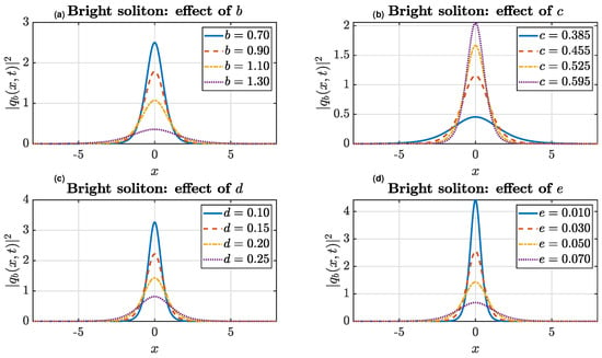
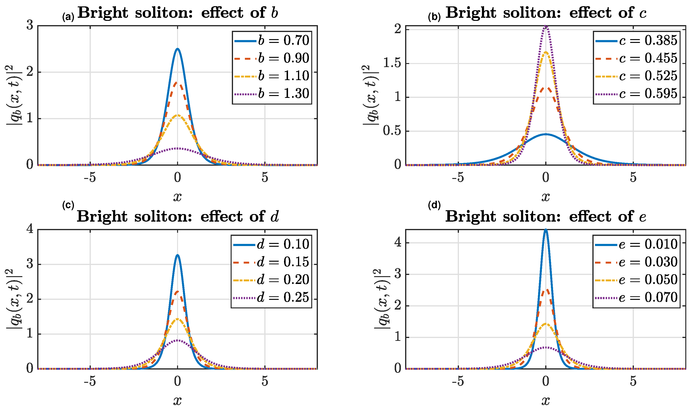
Two regular solitons were selected from the analytical catalog: the bright sech solution in Equation (21) and the dark tanh solution in Equation (34). The dark solution Equation (27) is not used here because its exact closure $d=-4e$ and $c=-eb/a$ makes the b–c and d–e continuations intrinsically paired. This explains the coincident trends obtained when that branch is plotted.

For these coefficient continuations, $a=1$ is fixed and exactly one of $b,c,d$, or e is changed in each panel, while the other three physical coefficients are held fixed. The frequency $\omega$ is treated as the nonlinear eigenvalue and is recomputed from the exact closure. The four panels therefore represent distinct coefficient continuations rather than relabelled versions of the same parameter path.

For the bright state, define

$$D=ab+(d+4e)\omega .$$

(55)

For $a>0$, $\omega >0$, and $D>0$, the regular Case 1 bright state is

$${|q_b(x,t)|}^2=A^2{\mathrm{sech}}^2\left(kx\right),A^2={\displaystyle \frac{2a\omega }{D}},k^2={\displaystyle \frac{\omega }{a}},$$

(56)

provided that

$$c={\displaystyle \frac{(d+3e)D}{a^2}}.$$

(57)

Solving this closure for the frequency gives

$${\omega }_b={\displaystyle \frac{c{a}^2/(d+3e)-ab}{d+4e}},(d+3e)(d+4e)\ne 0.$$

(58)

The bright-state baseline is $(a,b,c,d,e)=(1,1,0.49,0.20,0.05)$, for which ${\omega }_b=1$. The four continuations use $b\in [0.70,1.30]$, $c\in [0.385,0.595]$, $d\in [0.10,0.25]$, and $e\in [0.010,0.070]$. Because Equation (58) changes both A and k, the cubic, quintic, intensity-dependent-dispersion, and weakly nonlocal corrections produce visibly different peak-height and width responses. A quantitative width measure is the intensity full width at half maximum,

$$W_b={\displaystyle \frac{2\mathrm{arccosh}\left(\sqrt{2}\right)}{k}}.$$

(59)

The four parameter intervals are intentionally different because each is restricted to real, nondegenerate profiles satisfying the exact closure. Consequently, curve separations between different panels must not be interpreted as a ranking of the global coefficient sensitivity; the meaningful comparisons are the trends within a panel.

The bright-state coefficient continuations are displayed in Figure 1.

Figure 1. Effects of (a) b, (b) c, (c) d, and (d) e on the intensity of the exact bright soliton in Equation (21). The baseline is $(a,b,c,d,e)=(1,1,0.49,0.20,0.05)$, for which ${\omega }_b=1$. In each panel, $a=1$ is fixed, only the displayed physical coefficient varies, the other three are held at their baseline values, and ${\omega }_b$ is recomputed from the exact closure in Equation (58).

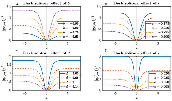
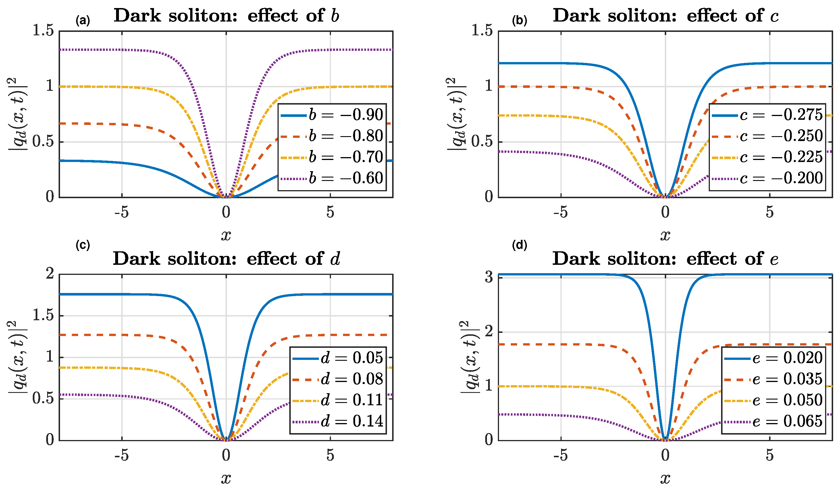
For the dark limit in Equation (34), we can write

$${|q_d(x,t)|}^2=A_d^2{\tanh }^2\left(k_{d}x\right),k_d^2={\displaystyle \frac{b-ac/(d+3e)}{2(d+4e)}},$$

(60)

where the remaining exact-closure quantities are

$$A_d^2=-{\displaystyle \frac{2(d+3e)k_d^2}{c}},{\omega }_d=-2a{k}_d^2+2e{A}_d^2{k}_d^2.$$

(61)

Real dark profiles require $A_d^2>0$, $k_d^2>0$, and nonzero denominators in Equations (60) and (61). The baseline $(a,b,c,d,e)=(1,-0.70,-0.25,0.10,0.05)$ gives $A_d^2=1$, $k_d^2=1/2$, and ${\omega }_d=-0.95$. The four independent ranges are $b\in [-0.90,-0.60]$, $c\in [-0.275,-0.200]$, $d\in [0.05,0.14]$, and $e\in [0.020,0.065]$. The resulting panels are no longer pairwise identical: b and c produce different background and notch scalings, while d and e display quantitatively distinct derivative-response trends because they enter the combinations $d+3e$ and $d+4e$ with different weights. The width of the region below half the background intensity is

$$W_d={\displaystyle \frac{2\mathrm{arctanh}(1/\sqrt{2})}{k_d}}.$$

(62)

As for the bright state, the intervals were selected only to preserve the exact closure and real nondegenerate profiles, so comparisons across panels are not global rankings of parameter influence.

The corresponding dark-state coefficient continuations are shown in Figure 2.

Figure 2. Effects of (a) b, (b) c, (c) d, and (d) e on the intensity of the exact dark soliton in Equation (34). The baseline is $(a,b,c,d,e)=(1,-0.70,-0.25,0.10,0.05)$, giving $A_d^2=1$, $k_d^2=1/2$, and ${\omega }_d=-0.95$. In each panel, $a=1$ is fixed, only the displayed coefficient varies, the other three are held at their baseline values, and ${\omega }_d$ is recomputed from the exact closure in Equation (61).

These profile continuations establish coefficient sensitivity and exact admissibility only. They do not constitute a stability result for the dark state; the spectral and propagation tests in the next subsection remain restricted to the representative bright state. Accordingly, no stability label is assigned to any untested analytical family. Stability-related numerical statements refer exclusively to the specified bright branch and to the resolution, domain, perturbation, and time interval stated for that test.

5.2.5. Branch-Specific Linear Spectral Test and Direct Finite-Time Perturbation Test

The residual calculations prove that the displayed profiles are exact solutions, but exactness alone does not determine whether a perturbed pulse remains observable. To examine both the amplitude and phase disturbances, let a regular quiescent profile $\varphi \left(x\right)$ be perturbed according to

$$q(x,t)=e^{i(\omega t+{\theta }_0)}\left[\varphi \left(x\right)+\epsilon \left(u(x,t)+iv(x,t)\right)\right],0<\epsilon \ll 1,$$

(63)

where u and v are independent real-valued perturbations. Substituting Equation (63) into Equation (1), followed by the retention of the $O\left(\epsilon \right)$ terms, gives

$${\displaystyle \frac{\partial }{\partial t}}\left(\begin{array}{c}u\\ v\end{array}\right)=\left(\begin{array}{cc}0& -{\mathcal{L}}_{-}\\ {\mathcal{L}}_{+}& 0\end{array}\right)\left(\begin{array}{c}u\\ v\end{array}\right)\equiv \mathcal{J}\left(\begin{array}{c}u\\ v\end{array}\right),$$

(64)

where

$${\mathcal{L}}_{-}f=(a+d{\varphi }^2)f_{xx}+\left[-\omega +b{\varphi }^2+c{\varphi }^4+e{\left({\varphi }^2\right)}_{xx}\right]f,$$

(65)

and

$$\begin{array}{cc}\hfill {\mathcal{L}}_{+}f=& (a+d{\varphi }^2)f_{xx}+2e\varphi {\left(\varphi f\right)}_{xx}\hfill \\ \hfill & +\left[-\omega +3b{\varphi }^2+5c{\varphi }^4+2d\varphi {\varphi }_{xx}+e{\left({\varphi }^2\right)}_{xx}\right]f.\hfill \end{array}$$

(66)

The signs in Equation (64) follow directly from the real and imaginary parts of $i(u_t+i{v}_t)$. In particular, $u_t=-{\mathcal{L}}_{-}v$ and $v_t={\mathcal{L}}_{+}u$.

With

$$\left(\begin{array}{c}u\\ v\end{array}\right)=e^{\lambda t}\left(\begin{array}{c}U\\ V\end{array}\right),$$

(67)

the spectral problem becomes

$$\lambda \left(\begin{array}{c}U\\ V\end{array}\right)=\mathcal{J}\left(\begin{array}{c}U\\ V\end{array}\right).$$

(68)

Spectral instability occurs if the spectrum contains an eigenvalue with $\mathrm{Re}\left(\lambda \right)>0$. For a bright state, the problem is posed on $L^2{\left(\mathbb{R}\right)}^2$ with decaying perturbations. The derivative nonlinearities modify the principal coefficients, so the nondegeneracy conditions in Equation (54) are required throughout the profile.

A representative regular bright state is obtained by selecting

$$a=1,\omega =1,b=1,c={\displaystyle \frac{1}{16}},d={\displaystyle \frac{1}{4}},e=-{\displaystyle \frac{1}{16}}.$$

(69)

This parameter set should be interpreted primarily as an internally consistent nondimensional mathematical benchmark rather than as a calibration to a specific optical material. The sign $d>0$ represents an intensity-dependent-dispersion correction that increases the envelope-curvature coefficient with intensity, whereas $e<0$ represents a weakly nonlocal curvature correction of the opposite sign. In coefficient magnitude, $\left|e\right|=1/16$ is one quarter of d and one sixteenth of a, so the nonlocal coefficient is subordinate to both the intensity-dependent and linear dispersive coefficients in this example. This ordering is compatible with a weak-correction regime at the dimensionless-model level, but no material-specific physical claim is made without an explicit dimensional scaling and parameter fit. The particular rational values in Equation (69) were chosen to provide a simple, reproducible benchmark on the exact regular bright branch rather than to fit a specific optical medium. They satisfy the Case 1 closure and give the elementary profile ${\varphi }_b=\sqrt{2}\mathrm{sech}x$, while also fulfilling the nondegeneracy requirement used in the first-integral construction, Equation (12): here, $d+2e=1/8$, so $a+(d+2e){\varphi }_b^2=1+\frac{1}{4}{\mathrm{sech}}^{2}x>0$ for all x. Moreover, $\left|e\right|<\left|d\right|<a$, which keeps the weakly nonlocal and intensity-dependent corrections subordinate to the linear dispersive scale. These features make the set convenient for isolating the numerical spectral and propagation accuracy without introducing a principal-coefficient degeneracy. These values give

$$({\Delta }_1,{\Delta }_2,{\Delta }_3,{\Delta }_4,{\Delta }_5)=\left({\displaystyle \frac{1}{8}},-{\displaystyle \frac{1}{8}},1,{\displaystyle \frac{1}{16}},-1\right),$$

(70)

and satisfy Equation (20). Hence,

$${\varphi }_b\left(x\right)=\sqrt{2}\mathrm{sech}x,q_b(x,t)=\sqrt{2}\mathrm{sech}x{e}^{it}.$$

(71)

For this profile, the phase- and amplitude-channel principal coefficients are, respectively,

$$a+d{\varphi }_b^2=1+{\displaystyle \frac{1}{2}}{\mathrm{sech}}^{2}x,a+(d+2e){\varphi }_b^2=1+{\displaystyle \frac{1}{4}}{\mathrm{sech}}^{2}x,$$

(72)

and are therefore strictly positive for all x.

As $\left|x\right|\to \infty$, ${\varphi }_b\to 0$ and ${\mathcal{L}}_{\pm }\to a{\partial }_x^2-\omega$. A Fourier mode $e^{i\xi x}$ consequently gives

$$\lambda =\pm i(a{\xi }^2+\omega ).$$

(73)

For Equation (69), the essential spectrum is

$${\sigma }_{\mathrm{ess}}\left(\mathcal{J}\right)=i(-\infty ,-1]\cup i[1,\infty ),$$

(74)

which lies on the imaginary axis. Phase and translation invariance generate the neutral directions ${(0,{\varphi }_b)}^T$ and ${({\varphi }_b^{\prime },0)}^T$ at $\lambda =0$.

The point spectrum was computed by Chebyshev collocation using standard spectral differentiation matrices [23]. On a domain $[-L,L]$, Chebyshev–Lobatto points were mapped from the standard interval and the first- and second-derivative matrices were scaled by $L^{-1}$ and $L^{-2}$, respectively. The boundary rows and columns were removed to impose homogeneous Dirichlet data, the variable coefficients were applied as diagonal matrices at the interior nodes, and the two resulting operators were assembled directly into the block matrix in Equation (64). The full dense block matrix was diagonalized with a standard QR-based LAPACK general eigensolver in IEEE 754 double precision (machine epsilon approximately $2.22\times {10}^{-16}$). Because a direct dense eigensolver was used, there was no iterative Krylov stopping tolerance; as an a posteriori accuracy check, computed eigenpairs were required to satisfy a normalized residual ${\parallel \mathcal{J}z-\lambda z\parallel }_2/({\parallel \mathcal{J}\parallel }_2{\parallel z\parallel }_2)<{10}^{-10}$. The distinction between a genuine unstable eigenvalue and numerical splitting was made by refinement rather than by a single real-part cutoff: a positive real part was regarded as unstable only if it converged to a nonzero positive value under both $N_c$ and L refinement. Near-zero eigenvalues that moved toward the origin with refinement and were associated with the phase- and translation-neutral subspace were classified as symmetry-induced numerical splitting.

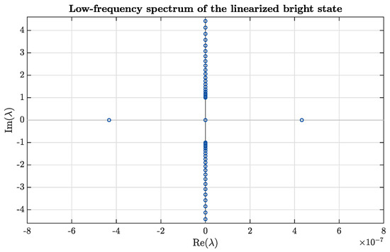
For $L=20$, Table 4 records the rightmost computed real part as the number $N_c$ of Chebyshev intervals is increased. The exact profile at the boundary has a magnitude of approximately $5.83\times {10}^{-9}$, so profile truncation is negligible on this scale. The small positive values are numerical splittings of the symmetry-generated zero eigenvalues and converge rapidly toward zero. At $N_c=260$, the rightmost real part is $4.29\times {10}^{-7}$, the neutral eigenvalues lie within $6.63\times {10}^{-7}$ of the origin, and the remaining low-frequency spectrum begins at $\left|\mathrm{Im}\lambda \right|\simeq 1.00247$, in agreement with the exact threshold $\left|\mathrm{Im}\lambda \right|=1$.

Table 4. Spectral convergence for the representative bright state (71).

Nc	max Re(λ)
180	$4.58\times {10}^{-4}$
220	$2.84\times {10}^{-5}$
240	$5.42\times {10}^{-6}$
260	$4.29\times {10}^{-7}$

Domain truncation was checked independently while keeping the density $N_c/L=13$ fixed. Table 5 shows that the rightmost splitting remains at the same numerical scale and that the first discrete approximation to the essential-spectrum edge approaches its exact value as the domain expands.

Table 5. Domain-size convergence for the representative bright state.

L	Nc	max Re(λ)	First |Imλ| Near the Edge
16	208	$4.33\times {10}^{-7}$	1.00630
18	234	$3.73\times {10}^{-7}$	1.00399
20	260	$4.29\times {10}^{-7}$	1.00247
22	286	$3.74\times {10}^{-7}$	1.00144
24	312	$3.52\times {10}^{-7}$	1.00070

Figure 3 shows the low-frequency spectrum at $N_c=260$. No eigenvalue with a positive real part survived resolution or domain refinement. Thus, no spectral instability was detected for the tested bright state within the stated numerical tolerances.

Figure 3. Low-frequency spectrum of the linearized block operator for the representative bright state (71), computed with $N_c=260$ Chebyshev intervals on $[-20,20]$. The spectrum is confined to the imaginary axis to numerical tolerance; the near-zero points are generated by phase and translation invariance.

To test the nonlinear evolution without preserving the exact profile by construction, the full PDE was initialized with simultaneous amplitude and phase disturbances,

$$q(x,0)={\varphi }_b\left(x\right)\left[1+\epsilon A_p\left(x\right)\right]e^{i\epsilon B_p\left(x\right)},\epsilon ={10}^{-2},$$

(75)

where

$$A_p\left(x\right)=0.8e^{-{(x/4)}^2}\cos \left(0.7x\right),B_p\left(x\right)=0.5e^{-{(x/5)}^2}\sin \left(0.9x\right).$$

(76)

The direct-evolution result below is deliberately restricted to this specified deterministic perturbation with $\epsilon ={10}^{-2}$. No amplitude sweep or broadband/random perturbation ensemble was used here; therefore, bounded propagation in this experiment does not establish robustness to arbitrary perturbation amplitudes or spectra and does not constitute proof of nonlinear orbital stability. For time integration, Equation (1) was written as

$$q_t=\mathcal{L}q+\mathcal{N}\left(q\right),\widehat{\mathcal{L}}\left(\zeta \right)=-ia{\zeta }^2,$$

(77)

with

$$\mathcal{N}\left(q\right)=i\left[bIq+c{I}^{2}q+dI{q}_{xx}+e{I}_{xx}q\right],I={\left|q\right|}^2.$$

(78)

The derivatives were evaluated by Fourier multipliers, all products were formed in physical space, and a two-thirds spectral filter was applied to the Fourier coefficients after every nonlinear evaluation. This is described as filtering, rather than exact de-aliasing, because the nonlinearity includes a quintic product.

The calculation used a periodic Fourier pseudospectral grid on $[-20,20]$ with $N=512$ modes and fourth-order exponential time differencing (ETDRK4) [24] with $\Delta t={10}^{-3}$ up to $T=20$. Repeating the calculation with $N=256$ and $\Delta t=2\times {10}^{-3}$ changed the final aligned error by less than $4.8\times {10}^{-12}$, the peak intensity by less than $2.4\times {10}^{-9}$, and the relative power change by less than $1.1\times {10}^{-12}$.

Because Equation (1) is invariant under constant phase rotations and spatial translations, the profile error was measured after removing these neutral motions:

$$E\left(t\right)=\underset{s,\vartheta \in \mathbb{R}}{\min }{\displaystyle \frac{{∥q(·,t)-e^{i(\omega t+\vartheta )}{\varphi }_b(·-s)∥}_2}{\parallel {\varphi }_b{\parallel }_2}}.$$

(79)

Numerically, the shift was selected by maximizing the magnitude of the periodic cross-correlation with the reference profile, and the phase was the argument of the corresponding complex inner product.

The relative physical-power variation was monitored through

$$\delta P\left(t\right)={\displaystyle \frac{P\left(t\right)-P\left(0\right)}{P\left(0\right)}},P\left(t\right)={\int }_{-\infty }^{\infty }{\left|q(x,t)\right|}^{2}dx.$$

(80)

Because P is not generally conserved when $d\ne 0$, this quantity is a physical pulse-content diagnostic rather than a time-stepping accuracy test. The accuracy was assessed by the stated space–time refinement and by the conserved generalized mass in Equation (10), for which

$$\delta {\mathcal{M}}_d\left(t\right)={\displaystyle \frac{{\mathcal{M}}_d\left(t\right)-{\mathcal{M}}_d\left(0\right)}{{\mathcal{M}}_d\left(0\right)}}.$$

(81)

On the periodic Fourier grid, ${\mathcal{M}}_d$ was evaluated with the composite periodic trapezoidal rule. For the tested bright state, $I_{\infty }=0$, so with $x_j=-L+j\Delta x$, $\Delta x=2L/N$, the discrete quantity is

$${\mathcal{M}}_d^{\left(h\right)}\left(t\right)={\displaystyle \frac{\Delta x}{d}}{\displaystyle \sum _{j=0}^{N-1}}\log \left|{\displaystyle \frac{a+d|q(x_j,t){|}^2}{a}}\right|.$$

(82)

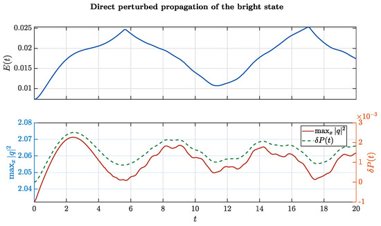
The same quadrature was used at every stored time, so the reported drift measures temporal/numerical conservation consistently on a fixed spatial grid. Over $0\le t\le 20$, the aligned error satisfied $E\left(t\right)\le 2.54\times {10}^{-2}$ and $E\left(20\right)=1.74\times {10}^{-2}$. The peak intensity remained in the interval $2.0321\le {\max }_x{\left|q\right|}^2\le 2.0713$, while $\left|\delta P\left(t\right)\right|\le 2.52\times {10}^{-3}$ and $|\delta {\mathcal{M}}_d\left(t\right)|\le 3.96\times {10}^{-13}$. The final common displacement was approximately $0.156$, consistent with the excitation of the neutral translation mode rather than pulse breakup.

The spectral refinement supports the absence of a detected spectral instability for the representative bright state (71), while the direct evolution shows a bounded finite-time response to the particular perturbation (75). This conclusion is parameter-, branch-, perturbation-, and time-window-specific: it is not a proof of nonlinear orbital stability for the full analytical family and does not extend to the kink, Jacobi elliptic, Weierstrass elliptic, or singular branches without separate background, Floquet, or singular-domain analyses.

The finite-time perturbation diagnostics for this representative bright state are summarized in Figure 4.

Figure 4. Phase-and-translation aligned shape error, peak intensity, and relative physical-power variation for the specified perturbed full-PDE propagation with $\epsilon ={10}^{-2}$. All plotted diagnostics remain bounded over $0\le t\le 20$ for this perturbation. The generalized-mass accuracy check, evaluated by Equation (82), satisfies $\left|\delta {\mathcal{M}}_d\right|\le 3.96\times {10}^{-13}$ (not plotted).

6. Conclusions

This study established a quiescent-wave reduction for a dimensionless cubic–quintic nonlinear Schrödinger equation that combines intensity-dependent dispersion with weak nonlocality. For a nonconstant real profile and nonzero intensity-dependent-dispersion coefficient, compatibility forces the carrier wavenumber and translation velocity to vanish. If that coefficient is zero, the same phase convention permits a moving branch, so the quiescent restriction is not universal outside the stated reduction.

The enhanced direct algebraic construction produces selected regular bright and dark states, singular hyperbolic states, and Jacobi and Weierstrass elliptic families. The shifted kink expressions are spatial translations and not new orbit types. Exactness is supported by the auxiliary equation, the six-part algebraic closure, direct stationary residuals, and an independent first integral. Explicit sign, reality, denominator, and principal-coefficient conditions separate admissible regular states from formal or singular expressions. The catalog is not claimed to be exhaustive.

Relative to the closest Kerr-only setting [10], the quintic response changes both the dominant balance and the coefficient manifolds required for closure. The parameter continuations show distinct within-panel responses of the cubic, quintic, dispersive, and weakly nonlocal coefficients. Because each continuation follows an exact closure over a different admissible interval, cross-panel curve separations are not global sensitivity rankings.

For one regular bright branch, both resolution and domain refinement removed the small positive splitting of the neutral eigenvalues, and no persistent unstable eigenvalue was detected. Full-equation propagation remained bounded through the tested finite interval for the specified simultaneous amplitude and phase perturbation with $\epsilon ={10}^{-2}$; this single test was not generalized to other perturbation amplitudes or spectra. The generalized mass was conserved to numerical precision, while ordinary optical power was used only as a physical diagnostic. These findings are branch-, parameter-, perturbation-, and time-window-specific. Stability of the dark, nonzero-background, periodic, Weierstrass, and singular families requires separate spectral settings and remains open.

References

- Agrawal, G.P. Nonlinear Fiber Optics, 6th ed.; Academic Press: Cambridge, MA, USA, 2019. [Google Scholar]
- Dai, C.Q.; Yang, Q.; He, J.D.; Wang, Y.Y. Nonlinear tunneling effect in the (2+1)-dimensional cubic–quintic nonlinear Schrödinger equation with variable coefficients. Eur. Phys. J. D. 2011, 63, 141–148. [Google Scholar] [CrossRef] [Scilit]
- Kengne, E.; Vaillancourt, R. Stability of exact solutions of the cubic–quintic nonlinear Schrödinger equation with periodic potential. Nonlinear Oscil. 2011, 13, 569–583. [Google Scholar] [CrossRef] [Scilit]
- Lin, C.-Y.; Chang, J.-H.; Kurizki, G.; Lee, R.-K. Solitons supported by intensity-dependent dispersion. Opt. Lett. 2020, 45, 1471–1474. [Google Scholar] [CrossRef] [Scilit] [PubMed]
- Ross, R.M.; Kevrekidis, P.G.; Pelinovsky, D.E. Localization in optical systems with an intensity-dependent dispersion. Q. Appl. Math. 2021, 79, 641–665. [Google Scholar] [CrossRef] [Scilit]
- Pelinovsky, D.E.; Ross, R.M.; Kevrekidis, P.G. Solitary waves with intensity-dependent dispersion: Variational characterization. J. Phys. A Math. Theor. 2021, 54, 445701. [Google Scholar] [CrossRef] [Scilit]
- Chang, J.-H.; Lin, C.-Y.; Lee, R.-K. Interplay between intensity-dependent dispersion and Kerr nonlinearity on the soliton formation. Opt. Lett. 2023, 48, 4249–4252. [Google Scholar] [CrossRef] [Scilit] [PubMed]
- Kevrekidis, P.G.; Pelinovsky, D.E.; Ross, R.M. Stability of smooth solitary waves under intensity-dependent dispersion. IMA J. Appl. Math. 2024, 89, 989–1005. [Google Scholar] [CrossRef] [Scilit]
- Pelinovsky, D.E.; Plum, M. Stability of black solitons in optical systems with intensity-dependent dispersion. SIAM J. Math. Anal. 2024, 56, 2521–2568. [Google Scholar] [CrossRef] [Scilit]
- Arnous, A.H.; Murad, M.A.S.; Moraru, L.; Yıldırım, Y.; Biswas, A. Quiescent optical solitons with nonlinear Schrödinger’s equation having Kerr law of self-phase modulation and intensity-dependent dispersion. Ain Shams Eng. J. 2026, 17, 104408. [Google Scholar] [CrossRef] [Scilit]
- Masalskyi, O.; Zharchenko, I.; Gradauskas, J. Peculiarities of hot carrier transport across GaAs p–n junctions under interband and intraband excitation. Ukr. J. Phys. Opt. 2026, 27, 03225–03237. [Google Scholar] [CrossRef] [Scilit]
- Królikowski, W.; Bang, O. Solitons in nonlocal nonlinear media: Exact solutions. Phys. Rev. E 2001, 63, 016610. [Google Scholar] [CrossRef] [Scilit] [PubMed]
- Zanga, D.; Fewo, S.I.; Tabi, C.B.; Kofané, T.C. Modulational instability in weak nonlocal nonlinear media with competing Kerr and non-Kerr nonlinearities. Commun. Nonlinear Sci. Numer. Simul. 2020, 80, 104993. [Google Scholar] [CrossRef] [Scilit]
- Triki, H.; Kruglov, V.I. Chirped periodic and localized waves in a weakly nonlocal media with cubic–quintic nonlinearity. Chaos Solitons Fractals 2021, 153, 111496. [Google Scholar] [CrossRef] [Scilit]
- Hosseini, K.; Sadri, K.; Hınçal, E.; Sirisubtawee, S.; Mirzazadeh, M. A generalized nonlinear Schrödinger involving the weak nonlocality: Its Jacobi elliptic function solutions and modulational instability. Optik 2023, 288, 171176. [Google Scholar] [CrossRef] [Scilit]
- Kudryashov, N.A. Stationary solitons of the generalized nonlinear Schrödinger equation with nonlinear dispersion and arbitrary refractive index. Appl. Math. Lett. 2022, 128, 107888. [Google Scholar] [CrossRef] [Scilit]
- Ouahid, L.; Abdou, M.A.; Alshahrani, D.O.; Akgül, A. New periodic wave solution for time-fractional perturbed nonlinear Schrödinger equation arising in optical fiber via newly extended mapping scheme. Opt. Rev. 2025, 32, 608–618. [Google Scholar] [CrossRef] [Scilit]
- Asjad, M.I.; Sagher, A.A.; Riaz, M.B.; Abdallah, S.A.O. Exploring optical soliton solution for (2+1)-dimensional Kundu–Mukherjee–Naskar equation using two analytical methods with sensitivity analysis. J. Korean Phys. Soc. 2026, 88, 352–369. [Google Scholar] [CrossRef] [Scilit]
- Afridi, M.I. Dynamical behaviours of soliton solutions with stability analysis to the q-deformed Tanh–Gordon model in optical fiber. Results Eng. 2025, 27, 106139. [Google Scholar] [CrossRef] [Scilit]
- Adem, A.R.; Arnous, A.H.; Calucag, L.S.; Biswas, A. Implicit quiescent soliton perturbation in optical metamaterials with nonlinear chromatic dispersion and Kudryashov’s quintuple form of self-phase modulation by Lie symmetry. Ukr. J. Phys. Opt. 2026, 27, 03009–03019. [Google Scholar] [CrossRef] [Scilit]
- Kaur, L.; Arnous, A.H.; Murad, M.A.S.; Biswas, A. Dispersive optical soliton perturbation with Schrödinger–Hirota equation by Lie symmetry. Ukr. J. Phys. Opt. 2026, 27, 03238–03258. [Google Scholar] [CrossRef] [Scilit]
- Arnous, A.H.; Murad, M.A.S.; Yıldırım, Y.; Biswas, A. Quiescent vector optical solitons with nonlinear dispersion. Ukr. J. Phys. Opt. 2026, 27, 04054–04076. [Google Scholar] [CrossRef] [Scilit]
- Trefethen, L.N. Spectral Methods in MATLAB; Society for Industrial and Applied Mathematics: Philadelphia, PA, USA, 2000. [Google Scholar] [CrossRef] [Scilit]
- Kassam, A.-K.; Trefethen, L.N. Fourth-order time-stepping for stiff PDEs. SIAM J. Sci. Comput. 2005, 26, 1214–1233. [Google Scholar] [CrossRef] [Scilit]
Disclaimer/Publisher’s Note: The statements, opinions and data contained in all publications are solely those of the individual author(s) and contributor(s) and not of MDPI and/or the editor(s). MDPI and/or the editor(s) disclaim responsibility for any injury to people or property resulting from any ideas, methods, instructions or products referred to in the content. |
© 2026 by the authors. Licensee MDPI, Basel, Switzerland. This article is an open access article distributed under the terms and conditions of the Creative Commons Attribution (CC BY) license.