Evaluation of a Subclass K_p,r = ∫x^p(1 + x²)^rdx of the Binomial Integral

Abstract

Employing the fundamental techniques of substitution, or change of variables, and integration by parts, the discussion in this paper focuses on obtaining explicit formulas for the integral $K_{p,r}=\int x^p{\left(1+x^2\right)}^{r}dx$ for $p\in \mathbb{Z}$ and $r\in \frac{1}{2}\mathbb{Z}$. As the case where r is a non-negative integer is rather simple and obvious, we concentrate mainly on the cases where r is a negative integer or an odd multiple of $\frac{1}{2}$ except when consideration of other cases is appropriate.

1. Preliminary

The traditional analytical approach for evaluating integrals relies on a toolkit of substitution and reduction formulas through integration by parts. The results of such derivations, accumulated and compiled over centuries, resulted in a large number of formulas and are now available in encyclopedic handbooks [1,2], which serve as the authoritative reference for practitioners seeking a specific solution.

In the meantime, the modern algorithmic approach is embodied by symbolic computation packages such as Maple [3] and Mathematica [4], which implement sophisticated procedures, for instance the Risch-Norman algorithm, to find antiderivatives automatically [5]. These packages are highly effective in practice and routinely succeed in integrals for which manual derivation would be prohibitively laborious. Their integration engines typically combine several distinct algorithms and extensive rule tables: however, the internal criteria governing which procedure is invoked for a given integral are generally not exposed to the user [6]. In essence, while immensely powerful, these packages offer limited insight into the analytical relationships between solutions, mathematical structure of the solutions, or a methodology for manual derivation.

The evaluation of definite integrals involving generalized hypergeometric functions [7,8] continues to be an active line of inquiry, as illustrated by a recent study that evaluates a broad class of such integrals by means of generalized Watson-type summation formulas [9]. In modern mathematical physics, related integrals with integer and half-integer parameters are frequently analyzed using harmonic polylogarithms [10] and special-function expansions, particularly in the study of Bessel-type functions [11] and Feynman integrals [12,13]. Another work combines integration-by-parts with differential equations to reduce parametrized families of Feynman integrals to a basis of master integrals, using a projective-geometry formulation in Feynman-parameter space [14]. A related generating-function approach has been used to solve integration-by-parts relations for a family of one-loop integrals indexed jointly by tensor structure and propagator-power distribution [15].

The evaluation of binomial integrals of the form $\int x^p{\left(a+b{x}^n\right)}^{r}dx$ is a classical problem in integral calculus with importance in physics and engineering [16,17]. The theoretical limits of this problem were established by Chebyshev, whose theorem delineates the specific conditions under which these integrals can be expressed in terms of elementary functions [18]. The subclass $K_{p,r}=\int x^p{\left(1+x^2\right)}^{r}dx$ of the binomial integrals constitutes a classical yet nontrivial problem in integral calculus, particularly when the parameters p and r extend beyond simple non-negative integers. Such cases arise naturally in various applications: for instance, the integral $K_{2,\frac{1}{2}}$ appears in the computation of surface areas of solids of revolution [19]. Some of the formulas in Sects. 2.110 and 2.27 of [2] can be interpreted as special cases of $K_{p,r}$.

Despite the breadth of existing results [1,20], several limitations remain apparent in both pedagogical and research-oriented treatments of the integral $K_{p,r}$. For instance, standard substitution techniques frequently lead to case-by-case calculations, which tend to obscure the underlying analytical structure of the solutions [19]. In addition, reduction formulas obtained through integration by parts often encounter ‘walls’ that interrupt recursive evaluation, requiring problem-dependent initial conditions. Furthermore, although closed-form expressions are available for many individual cases, these results are typically scattered across tables or derived in isolation [1,2] A unification effort has recently been undertaken for another classical family of parametrized integrals, Lobachevsky’s integrals, by combining parameter differentiation, partial fraction decomposition, and series expansion into a single systematic derivation covering all convergent cases [21], underscoring the continuing value of organizing scattered classical results within one coherent analytical framework.

In this paper, we develop a unified analytical and recursive framework for the systematic evaluation of $K_{p,r}$. The approach in this paper is based on a detailed analysis of the parameter plane $(p,r)$. We identify five lines $p=1$, $p=-1$, $r=0$, $r=-1$, and $p+2r+3=0$ along which the integral admits direct closed-form evaluation. These cases provide a natural set of initial conditions that anchor the recursive structure of the problem. Building upon these initial conditions, we derive four general recursion formulas that enable the evaluation of $K_{p,r}$ at any admissible point in the parameter plane while systematically bypassing the recursion barriers encountered, mostly on the line $p+2r+1=0$, in conventional approaches.

The main contributions of this work can be summarized as follows:

• The parameter plane of $(p,r)$ is systematically grouped to provide a unified analytical framework for the categorization and derivation of $K_{p,r}$. Five fundamental lines are identified upon which the integral $K_{p,r}$ can be evaluated directly to serve as the foundational initial conditions.
• Four recursion formulas are derived that enable the methodical generation of solutions at any admissible point $(p,r)$.
• Recursive stability is ensured by systematically bypassing traditional recursion walls with a complete and sufficient set of initial conditions.
• This work culminates in a compendium of explicit, closed-form formulas, serving as a valuable reference.

2. Evaluation of $K_{p,r}$ with Basic Techniques

In this paper, our focus will be on obtaining explicit formulas for the primitive function or antiderivative $K_{p,r}$ of $x^p{\left(1+x^2\right)}^r$ in the real domain, intervals of x avoiding $x=0$. Specifically, explicit formulas for

$$K_{p,r}=\int x^p{\left(1+x^2\right)}^{r}dx$$

(1)

on every point $(p,r)$ in the set

$${\mathsf{\Omega }}_K=\left\{(p,r):p\in \mathbb{Z},r\in \frac{1}{2}\mathbb{Z}\right\}$$

(2)

of admissible points will be derived with the main focus on the cases where r is a negative integer or an odd multiple of $\frac{1}{2}$. Apparently, among the binomial integrals [16,17]

$$\int x^p{\left(a+b{x}^n\right)}^{r}dx,$$

(3)

where $a,b\in \mathbb{R}$ and $p,n,r\in \mathbb{Q}$, the integral $K_{p,r}$ considered in this paper is a subclass with $a=b$, $n=2$, and $(p,r)\in {\mathsf{\Omega }}_K$. It should be noted that (2) implies the existence of $K_{p,r}$ in terms of elementary functions by the theorem of Chebyshev [18] because r, $\frac{p+1}{2}$, and/or $\frac{p+1}{2}+r$ will be an integer for every point $(p,r)$ in the set ${\mathsf{\Omega }}_K$.

Throughout the paper, except when necessary, integration constants will be omitted for brevity. From time to time, the terms antiderivative, primitive function, explicit formula, and integral will be used interchangeably with $K_{p,r}$ and explicit formula for the integral, which would not incur too much confusion.

2.1. Evaluation via Substitution

With $x=\tan \theta$ and $1+x^2=t$, we have

$$K_{p,r}=\int \frac{{sin}^p\theta }{{cos}^{p+2r+2}\theta }d\theta$$

(4)

and

$$K_{p,r}=\frac{1}{2}\int {(t-1)}^{\frac{p-1}{2}}{t}^{r}dt,$$

(5)

respectively. In addition, with $\sqrt{1+x^2}=t$, we obtain

$$K_{p,r}=\int {\left(t^2-1\right)}^{\frac{p-1}{2}}{t}^{2r+1}dt,$$

(6)

similar to (5) but more useful, especially when r is an integral multiple of $\frac{1}{2}$.

Example 1. 

When $p=0$, using (4), we can obtain $K_{0,-\frac{1}{2}}=\ln \left(x+\sqrt{1+x^2}\right)$, $K_{0,-1}={\tan }^{-1}x$, and $K_{0,-\frac{3}{2}}=\frac{x}{\sqrt{1+x^2}}$. In addition, (4) can also be used to obtain

$$K_{1,-1}=\frac{1}{2}\ln \left(1+x^2\right)$$

(7)

and

$$K_{-1,-1}=\frac{1}{2}\ln \frac{x^2}{1+x^2}.$$

(8)

Similarly, the result (5) can be used to obtain $K_{3,-2}=\frac{1}{2}\left\{\ln \left(1+x^2\right)+\frac{1}{1+x^2}\right\}$, for instance. In addition, we can obtain $K_{1,-\frac{1}{2}}=\sqrt{1+x^2}$ and $K_{-1,-\frac{1}{2}}=\frac{1}{2}\ln \frac{\sqrt{1+x^2}-1}{\sqrt{1+x^2}+1}$ with (6) after some steps.

2.2. Evaluation via Integration by Parts

When $(p,r)=(-1,0)$, it is easy to see that $K_{-1,0}=\int \frac{dx}{x}$ or

$$K_{-1,0}=\ln \left|x\right|.$$

(9)

Next, when $p\ne -1$, with $u^{\prime }=x^p$, $v={\left(1+x^2\right)}^r$, $u=\frac{x^{p+1}}{p+1}$, and $v^{\prime }=2rx{\left(1+x^2\right)}^{r-1}$, we obtain

$$K_{p,r}=\frac{x^{p+1}{\left(1+x^2\right)}^r}{p+1}-\frac{2r}{p+1}\int x^{p+2}{\left(1+x^2\right)}^{r-1}dx.$$

(10)

Rewriting (10), we have

$$K_{p,r}=\frac{x^{p+1}}{p+1}{\left(1+x^2\right)}^r-\frac{2r}{p+1}{K}_{p,r}+\frac{2r}{p+1}{K}_{p,r-1}.$$

(11)

First, when $-\frac{2r}{p+1}=1$ in (11), we obtain $0=\frac{x^{p+1}{\left(1+x^2\right)}^r}{p+1}+\frac{2r}{p+1}{K}_{p,r-1}$ or

$$K_{p,-\frac{p+3}{2}}=\frac{x^{p+1}}{p+1}{\left(1+x^2\right)}^{-\frac{p+1}{2}}$$

(12)

for $p\ne -1$. On the other hand, when $-\frac{2r}{p+1}\ne 1$, we obtain $\left(1+\frac{2r}{p+1}\right)K_{p,r}=\frac{x^{p+1}{\left(1+x^2\right)}^r}{p+1}+\frac{2r}{p+1}{K}_{p,r-1}$, which can be expressed as

$$K_{p,r}=\frac{x^{p+1}{\left(1+x^2\right)}^r}{p+2r+1}+\frac{2r}{p+2r+1}{K}_{p,r-1}$$

(13)

for $p+2r+1\ne 0$ and $p\ne -1$. Although we assumed $p\ne -1$ from the starting point of (10), the result (13) holds for $p=-1$ also, producing

$$K_{-1,r}=\frac{1}{2r}{\left(1+x^2\right)}^r+K_{-1,r-1}$$

(14)

for $r\ne 0$.

Similarly, when $r\ne -1$, with $u=x^{p-1}$, $v^{\prime }=x{\left(1+x^2\right)}^r$, $u^{\prime }=(p-1)x^{p-2}$, and $v=\frac{{\left(1+x^2\right)}^{r+1}}{2(r+1)}$, we obtain

$$K_{p,r}=\frac{x^{p-1}}{2(r+1)}{\left(1+x^2\right)}^{r+1}-\frac{p-1}{2(r+1)}\int x^{p-2}{\left(1+x^2\right)}^{r+1}dx.$$

(15)

If $p=1$, we easily obtain

$$K_{1,r}=\frac{{\left(1+x^2\right)}^{r+1}}{2(r+1)}$$

(16)

for $r\ne -1$ from (15): for $r=-1$, recollect $K_{1,-1}=\frac{1}{2}\ln \left(1+x^2\right)$ shown in (7).

Subsequently, (15) can be expressed as

$$K_{p,r}=\frac{x^{p-1}}{2(r+1)}{\left(1+x^2\right)}^{r+1}-\frac{p-1}{2(r+1)}{K}_{p,r}-\frac{p-1}{2(r+1)}{K}_{p-2,r}.$$

(17)

First, when $-\frac{p-1}{2(r+1)}=1$ and $r\ne -1$, we obtain $0=\frac{x^{p-1}}{2(r+1)}{\left(1+x^2\right)}^{r+1}-\frac{p-1}{2(r+1)}{K}_{p-2,r}$ or equivalently $K_{p-2,-\frac{p+1}{2}}=\frac{x^{p-1}}{p-1}{\left(1+x^2\right)}^{-\frac{p-1}{2}}$ for $p\ne 1$: this result is the same as (12) when p is replaced with $p+2$. Next, when $-\frac{p-1}{2(r+1)}\ne 1$ and $r\ne -1$, we obtain $\left\{1+\frac{p-1}{2(r+1)}\right\}{K}_{p,r}=\frac{x^{p-1}}{2(r+1)}{\left(1+x^2\right)}^{r+1}-\frac{p-1}{2(r+1)}{K}_{p-2,r}$, or

$$K_{p,r}=\frac{x^{p-1}{\left(1+x^2\right)}^{r+1}}{p+2r+1}-\frac{p-1}{p+2r+1}{K}_{p-2,r}$$

(18)

for $p+2r+1\ne 0$ and $r\ne -1$. When $p=1$, (18) is the same as (16). In (15), we have assumed $r\ne -1$: yet, (18) holds true for $r=-1$ also, producing

$$K_{p,-1}=\frac{x^{p-1}}{p-1}-K_{p-2,-1}.$$

(19)

Example 2. 

When $p=0$ and $r=-\frac{1}{2}$, we obtain $K_{0,-\frac{1}{2}}=\frac{x}{\sqrt{1+x^2}}+K_{2,-\frac{3}{2}}$ from (10). Thus, $K_{2,-\frac{3}{2}}=K_{0,-\frac{1}{2}}-\frac{x}{\sqrt{1+x^2}}$ or

$$K_{2,-\frac{3}{2}}=\ln \left(x+\sqrt{1+x^2}\right)-\frac{x}{\sqrt{1+x^2}}$$

(20)

using the results $K_{0,-\frac{1}{2}}=\ln \left(x+\sqrt{1+x^2}\right)$ shown in Example 1. In addition, from (13), we have $K_{2,-\frac{1}{2}}=\frac{x^3}{2\sqrt{1+x^2}}-\frac{1}{2}{K}_{2,-\frac{3}{2}}=\frac{x^3+x}{2\sqrt{1+x^2}}-\frac{1}{2}\ln \left(x+\sqrt{1+x^2}\right)$ and subsequently $K_{2,\frac{1}{2}}=\frac{x^3}{4}\sqrt{1+x^2}+\frac{1}{4}{K}_{2,-\frac{1}{2}}=\frac{2x^5+3x^3+x}{8\sqrt{1+x^2}}-\frac{1}{8}\ln \left(x+\sqrt{1+x^2}\right)$. We also have $K_{0,-\frac{3}{2}}=-\frac{1}{2x\sqrt{1+x^2}}-\frac{1}{2}{K}_{-2,-\frac{3}{2}}$ from (18), and thus $K_{-2,-\frac{3}{2}}=-\frac{1}{x\sqrt{1+x^2}}-2K_{0,-\frac{3}{2}}=-\frac{2x^2+1}{x\sqrt{1+x^2}}$ with $K_{0,-\frac{3}{2}}=\frac{x}{\sqrt{1+x^2}}$ shown in Example 1.

3. Derivation of Explicit Formulas

In the following developments, ${\displaystyle \prod _{a=b}^c}$ and ${\displaystyle \sum _{a=b}^c}$ denote the product and sum, respectively, for $a=b,b+1,b+2,\cdots ,c$ even when b and c are not integers. To denote ‘$k=p,p+2,\cdots$’, we use ‘$k=p:2$’ especially for the lower limit of a summation. We also let ${\displaystyle \sum _{a=b}^c}g\left(a\right)=0$ and ${\displaystyle \prod _{a=b}^c}h\left(a\right)=1$ if $c<b$. In addition, $(p,r)$ often implies $K_{p,r}$ also. Again, integral constants will be omitted unless they are essential.

3.1. Explicit Formulas for $p=\pm 1$, $r=0$, $r=-1$, and $p+2r+3=0$

We first consider the cases in which direct evaluation of explicit formulas is possible.

Lemma 1. 

For $r=0$, we easily obtain

$$K_{p,0}=\left\{\begin{array}{cc}\ln \left|x\right|,\hfill & p=-1,\hfill \\ \frac{x^{p+1}}{p+1},\hfill & p\ne -1.\hfill \end{array}\right.$$

(21)

Next, by combining the results shown in (7) and (16), we have

$$K_{1,r}=\left\{\begin{array}{cc}\frac{1}{2}\ln \left(1+x^2\right),\hfill & r=-1,\hfill \\ \frac{{\left(1+x^2\right)}^{r+1}}{2(r+1)},\hfill & r\ne -1\hfill \end{array}\right.$$

(22)

for $p=1$. Similarly, collecting the results shown in (8) and (12), we have

$$K_{p,-\frac{p+3}{2}}=\left\{\begin{array}{cc}\frac{1}{2}\ln \frac{x^2}{1+x^2},\hfill & p=-1,\hfill \\ \frac{x^{p+1}}{p+1}{\left(1+x^2\right)}^{-\frac{p+1}{2}},\hfill & p\ne -1\hfill \end{array}\right.$$

(23)

for $p+2r+3=0$.

Theorem 1. 

For $p=-1$, as shown in (A7) of Appendix A.1, the explicit formulas for $K_{-1,r}$ can be expressed as

$$K_{-1,r}=\left\{\begin{array}{c}\frac{1}{2}\left\{\ln \left|v_r\left(x\right)\right|+{\displaystyle \sum _{k=1}^{h_{2r+1}}}\left(\genfrac{}{}{0pt}{}{h_{2r+1}}{k}\right)\frac{v_r^k\left(x\right)}{k}\right\},\hfill \\ r=0,\pm 1,\cdots ,\hfill \\ \frac{1}{2}\left\{\ln \frac{\sqrt{1+x^2}-1}{\sqrt{1+x^2}+1}+{\displaystyle \sum _{k=0}^{h_{2r+1}-\frac{1}{2}}}\frac{{\left(1+x^2\right)}^{k_{2r+1}{s}_r}}{k_{2r+1}}\right\},\hfill \\ r=\pm \frac{1}{2},\pm \frac{3}{2},\cdots ,\hfill \end{array}\right.$$

(24)

where $h_y=\frac{1}{2}\left(\right|y|-1)$, $k_y=h_y-k$,

$$v_y\left(x\right)=\left\{\begin{array}{cc}{x}^2,\hfill & y=0,1,\dots ,\hfill \\ \frac{-x^2}{1+x^2},\hfill & y=-1,-2,\cdots ,\hfill \end{array}\right.$$

(25)

and

$$s_y=\left\{\begin{array}{cc}1,\hfill & y\ge 0,\hfill \\ -1,\hfill & y<0\hfill \end{array}\right.$$

(26)

denotes the sign of y: note that $s_0=1$, not $s_0=0$.

Example 3. 

With (24), we obtain $K_{-1,-2}=\frac{1}{2}\ln \left|v_{-2}\left(x\right)\right|+\frac{1}{2}{v}_{-2}\left(x\right)=\frac{1}{2}\left(\ln \frac{x^2}{1+x^2}-\frac{x^2}{1+x^2}\right)$, for instance.

Theorem 2. 

For $r=-1$, the explicit formulas for $K_{p,-1}$ can be expressed as

$$K_{p,-1}=\left\{\begin{array}{c}\frac{s_p}{2}{(-1)}^{h_p+\frac{1}{2}}\left\{2{\tan }^{-1}{x}^{s_p}+{\displaystyle \sum _{k=1}^{h_p+\frac{1}{2}}}\frac{{(-1)}^{k_p-\frac{1}{2}}}{k_p+1}{x}^{2(k_p+1)s_p}\right\},\hfill \\ p=0,\pm 2,\pm 4\cdots ,\hfill \\ \frac{s_p}{2}{(-1)}^{h_p}\left\{\ln \left(1+x^{2s_p}\right)+{\displaystyle \sum _{k=1}^{h_p}}\frac{{(-1)}^k}{k}\left(\genfrac{}{}{0pt}{}{h_p}{k}\right){\left(1+x^{2s_p}\right)}^k\right\},\hfill \\ p=\pm 1,\pm 3,\cdots \hfill \end{array}\right.$$

(27)

as shown in (A15) of Appendix A.2.

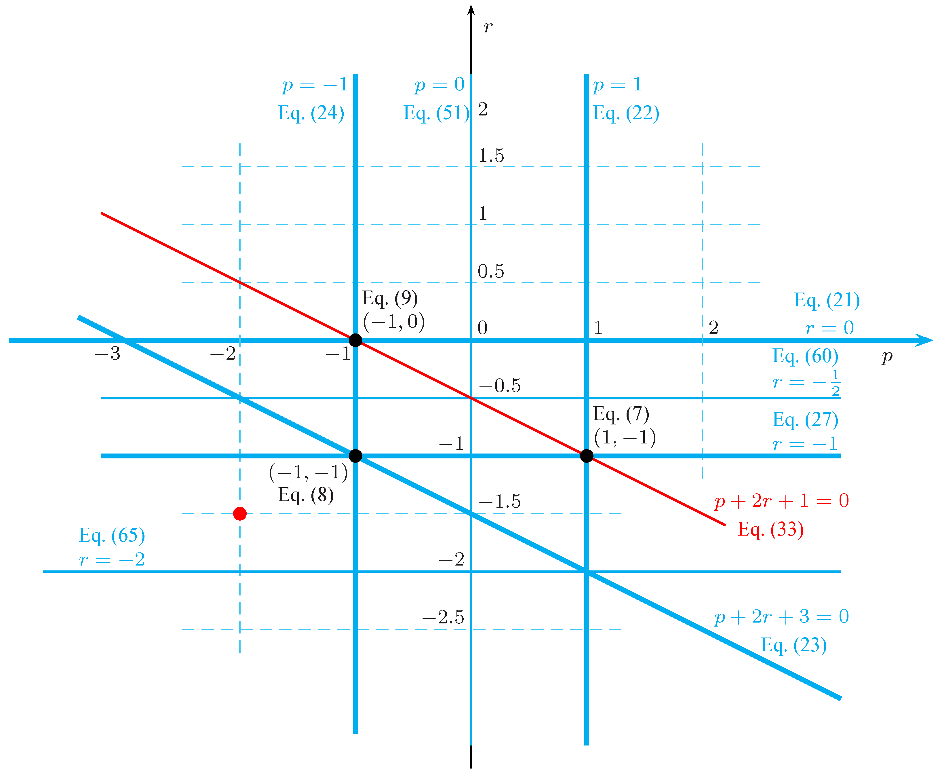
The results (21)–(24) and (27) allow us to obtain the explicit formulas for the integral $K_{p,r}$ for every point $(p,r)\in {\mathsf{\Omega }}_K$ in the five lines $r=0$, $p=1$, $p+2r+3=0$, $p=-1$, and $r=-1$, respectively. Figure 1 illustrates the five lines in which every point now has an explicit formula for the integral $K_{p,r}$: three additional lines are also included based on the results later in this section.

3.2. Explicit Formulas when $p+2r+1=0$

If $\{p+2r+1=0\}\cap \{p=-1\}$, we easily obtain $K_{-1,0}=\int \frac{1}{x}dx=\ln \left|x\right|$ as discussed in (9) also. For $\{p+2r+1=0\}\cap \{p\ne -1\}$, we can obtain $K_{p,-\frac{p+1}{2}}$ from $K_{p+2,-\frac{p+3}{2}}$ or vice versa for $p=0,\pm 1,\pm 2,\cdots$ with the recursion

$$K_{p,-\frac{p+1}{2}}=\frac{x^{p+1}}{p+1}{\left(1+x^2\right)}^{-\frac{p+1}{2}}+K_{p+2,-\frac{p+3}{2}},$$

(28)

which can be derived from (10) or (15).

When using the recursion (28), two initial conditions, known formulas for $K_{p,r}$ in this paper, are required because the recursion describes a relationship between two $K_{p,r}$’s with a difference of 2 in the subscript p and we assume integers for p. In addition, due to the ‘wall’ effect that neither $K_{-1,0}$ from $K_{1,-1}$ nor $K_{1,-1}$ from $K_{-1,0}$ can be obtained when $p=-1$ caused by the factor $p+1$ in the denominator on the right-hand side of (28), one additional initial condition is required.

In short, for the recursion (28), a complete set of three initial conditions would be $\left\{K_{1,-1},K_{0,-\frac{1}{2}},K_{-1,0}\right\}$, of which the first, second, and third elements can be replaced by any element from $\left\{K_{2m-1,-m}:m=1,2,\cdots \right\}$, $\left\{K_{2m,-m-\frac{1}{2}}:m=0,\pm 1,\pm 2,\cdots \right\}$, and $\left\{K_{2m-1,-m}:m=0,-1,-2,\cdots \right\}$, respectively.

Now, by adding

$$\begin{array}{cc}\hfill K_{p,-\frac{p+1}{2}}& =\frac{x^{p+1}}{p+1}{\left(1+x^2\right)}^{-\frac{p+1}{2}}+K_{p+2,-\frac{p+3}{2}},\hfill \end{array}$$

(29)

$$\begin{array}{cc}\hfill K_{p+2,-\frac{p+3}{2}}& =\frac{x^{p+3}}{p+3}{\left(1+x^2\right)}^{-\frac{p+3}{2}}+K_{p+4,-\frac{p+5}{2}},\hfill \\ \hfill & ⋮\hfill \end{array}$$

(30)

$$\begin{array}{cc}\hfill K_{s-2,-\frac{s-1}{2}}& =\frac{x^{s-1}}{s-1}{\left(1+x^2\right)}^{-\frac{s-1}{2}}+K_{s,-\frac{s+1}{2}},\hfill \end{array}$$

(31)

obtained from (28), we obtain

$$K_{p,-\frac{p+1}{2}}=K_{s,-\frac{s+1}{2}}+{\displaystyle \sum _{k=p:2}^{s-2}}\frac{x^{k+1}}{k+1}{\left(1+x^2\right)}^{-\frac{k+1}{2}}$$

(32)

for $s=p+2m$ with m a positive integer. It is easy to see that the result (32) can also be used for $s=p+2m$ with m a negative integer after an interchange of the subscripts p and s. Subsequently, the initial conditions $K_{0,-\frac{1}{2}}=\ln \left(x+\sqrt{1+x^2}\right)$ from Example 1, $K_{1,-1}=\frac{1}{2}\ln \left(1+x^2\right)$ from (7), and $K_{-1,0}=\ln \left|x\right|$ from (9) can be used to obtain $K_{p,-\frac{p+1}{2}}$ recursively for $p=\pm 2,\pm 4,\cdots$, for $p=3,5,\cdots$, and for $p=-3,-5,\cdots$, respectively. These observations will lead us to the following theorem.

Theorem 3. 

The explicit formulas for $K_{p,-\frac{p+1}{2}}$ can be obtained via

$$K_{p,-\frac{p+1}{2}}=v_{p,-\frac{p+1}{2}}\left(x\right)+{\displaystyle \sum _{k=L_{p,-\frac{p+1}{2}}:2}^{U_{p,-\frac{p+1}{2}}}}{w}_{p,-\frac{p+1}{2},k}\left(x\right),$$

(33)

where

$$L_{p,-\frac{p+1}{2}}=\left\{\begin{array}{cc}0,\hfill & p=0,2,\cdots ,\hfill \\ 1,\hfill & p=1,3,\cdots ,\hfill \\ p,\hfill & p=-1,-2,\cdots \hfill \end{array}\right.$$

(34)

denotes the lower limit of the summation,

$$U_{p,-\frac{p+1}{2}}=\left\{\begin{array}{cc}p-2,\hfill & p=1,2,\cdots ,\hfill \\ -3,\hfill & p=-1,-3,\cdots ,\hfill \\ -2,\hfill & p=0,-2,-4,\cdots \hfill \end{array}\right.$$

(35)

denotes the upper limit of the summation,

$$v_{p,-\frac{p+1}{2}}\left(x\right)=\left\{\begin{array}{cc}\ln \sqrt{1+x^2},\hfill & p=1,3,\cdots ,\hfill \\ \ln \left|x\right|,\hfill & p=-1,-3,\cdots ,\hfill \\ \ln \left(x+\sqrt{1+x^2}\right),\hfill & p=0,\pm 2,\pm 4,\cdots ,\hfill \end{array}\right.$$

(36)

and

$$w_{p,-\frac{p+1}{2},k}\left(x\right)=-\frac{s_p}{k+1}{x}^{k+1}{\left(1+x^2\right)}^{-\frac{k+1}{2}}$$

(37)

for the points $(p,r)$ on the line $p+2r+1=0$.

Example 4. 

We obtain $K_{3,-2}=\frac{1}{2}\ln \left(1+x^2\right)-\frac{x^2}{2\left(1+x^2\right)}$, $K_{5,-3}=\frac{1}{2}\ln \left(1+x^2\right)-\frac{x^2}{2\left(1+x^2\right)}-\frac{x^4}{4{\left(1+x^2\right)}^2}$, $K_{2,-\frac{3}{2}}=\ln \left(x+\sqrt{1+x^2}\right)-\frac{x}{\sqrt{1+x^2}}$, and $K_{-2,\frac{1}{2}}=\ln \left(x+\sqrt{1+x^2}\right)-\frac{\sqrt{1+x^2}}{x}$ from (33). We also easily obtain $K_{-3,1}=\ln \left|x\right|-\frac{1+x^2}{2x^2}$ and $K_{-5,3}=\ln \left|x\right|-\frac{1+x^2}{2x^2}-\frac{{\left(1+x^2\right)}^2}{4x^4}$.

3.3. Explicit Formulas on Other Points of $(p,r)$

To obtain $K_{p,r}$ from $K_{p,r-1}$ or vice versa at every admissible value $r=0,\pm \frac{1}{2},\pm 1,\dots$ except $r=-\frac{p+1}{2}$ when p is fixed, we can use

$$K_{p,r}=\frac{x^{p+1}{\left(1+x^2\right)}^r}{p+2r+1}+\frac{2r}{p+2r+1}{K}_{p,r-1}$$

(38)

shown in (13). Similarly, to obtain $K_{p,r}$ from $K_{p-2,r}$ or vice versa at every admissible value $p=0,\pm 1,\pm 2,\dots$ except $p=-2r-1$ when r is fixed, we can use

$$K_{p,r}=\frac{x^{p-1}{\left(1+x^2\right)}^{r+1}}{p+2r+1}-\frac{p-1}{p+2r+1}{K}_{p-2,r}$$

(39)

shown in (18).

The recursion (38) allows us to obtain $K_{p,r}$ from $K_{p,r-1}$ and vice versa in general: however, when $r=0$ and $r=-\frac{p+1}{2}$, neither $K_{p,r}$ from $K_{p,r-1}$ nor $K_{p,r-1}$ from $K_{p,r}$ can be obtained. Based on this observation, we divide the points in ${\mathsf{\Omega }}_K$ into three groups such that $r\in G_{p,L}$, $r\in G_{p,B}$, and $r\in G_{p,U}$, where $G_{p,L}=\left(-\infty ,r_L-\frac{1}{2}\right]$, $G_{p,B}=\left[r_L,r_U-\frac{1}{2}\right]$, and $G_{p,U}=\left[r_U,\infty \right)$ are called the group sets of r with $r_L=min\left(-\frac{p+1}{2},0\right)$ and $r_U=max\left(-\frac{p+1}{2},0\right)$. Likewise, when obtaining $K_{p,r}$ from $K_{p,r-1}$ and vice versa with (39), we define three group sets of p, $G_{L,r}=\left(-\infty ,p_L-1\right]$, $G_{B,r}=\left[p_L,p_U-1\right]$, and $G_{U,r}=\left[p_U,\infty \right)$, where $p_L=min\left(-2r-1,1\right)$ and $p_U=max\left(-2r-1,1\right)$.

Clearly, the two recursions (38) and (39) require initial conditions, the known formulas for $K_{p,r}$: for instance, those on the admissible points in the six lines $r=0$, $p=1$, $p=-1$, $r=-1$, $p+2r+1=0$, and $p+2r+3=0$ will naturally be the candidates as the initial conditions. Appendix A.7 provides more detailed discussion on the issue of initial conditions.

3.3.1. Derivation of $K_{p,r}$ via (38) for $p\ne -1$ Fixed

Let

$$a_{p,r}\left(x\right)=\frac{x^{p+1}{\left(1+x^2\right)}^r}{p+2r+1}$$

(40)

and

$$b_{p,r}=\frac{2r}{p+2r+1}.$$

(41)

Then, if we add

$$\begin{array}{cc}\hfill K_{p,r}& =a_{p,r}\left(x\right)+b_{p,r}{K}_{p,r-1}\hfill \end{array}$$

(42)

$$\begin{array}{cc}\hfill b_{p,r}{K}_{p,r-1}& =b_{p,r}{a}_{p,r-1}\left(x\right)+b_{p,r}{b}_{p,r-1}{K}_{p,r-2}\hfill \end{array}$$

(43)

$$\begin{array}{cc}\hfill b_{p,r}{b}_{p,r-1}{K}_{p,r-2}& =b_{p,r}{b}_{p,r-1}{a}_{p,r-2}\left(x\right)+b_{p,r}{b}_{p,r-1}{b}_{p,r-2}{K}_{p,r-3}\hfill \\ \hfill & ⋮\hfill \end{array}$$

(44)

$$\begin{array}{cc}\hfill K_{p,s+1}{\displaystyle \prod _{m=s+2}^r}{b}_{p,m}& =a_{p,s+1}\left(x\right){\displaystyle \prod _{m=s+2}^r}{b}_{p,m}+K_{p,s}{\displaystyle \prod _{m=s+1}^r}{b}_{p,m}\hfill \end{array}$$

(45)

we obtain

$$K_{p,r}={\displaystyle \sum _{k=s+1}^r}{a}_{p,k}\left(x\right){\displaystyle \prod _{m=k+1}^r}{b}_{p,m}+K_{p,s}{\displaystyle \prod _{m=s+1}^r}{b}_{p,m}$$

(46)

for $r>s$.

Now, note that ${\displaystyle \prod _{m=k+1}^r}{b}_{p,m}=\frac{2k+2}{p+2k+3}\frac{2k+4}{p+2k+5}\cdots \frac{2r}{p+2r+1}=\frac{\left(2r\right)!!(p+2k+1)!!}{(p+2r+1)!!\left(2k\right)!!}=\frac{S(p,r)}{S(p,k)}$, where

$$S(a,b)=\frac{\left(2b\right)!!}{(a+2b+1)!!}$$

(47)

with the double factorial defined as

$$k!!=\left\{\begin{array}{cc}-1,\hfill & ifk=-2,\hfill \\ 1,\hfill & ifk=-1,0,\hfill \\ k(k-2)!!,\hfill & ifk=1,2,\dots ,\hfill \\ \frac{(k+2)!!}{k+2},\hfill & ifk=-3,-4,\dots .\hfill \end{array}\right.$$

(48)

Some values of the double factorial $k!!$ are shown in

Table 1. Some values of $k!!$.

$\mathit{k}$	⋯	9	8	7	6	5	4	3	2	1	0
$k!!$	⋯	945	384	105	48	15	8	3	2	1	1
$\mathit{k}$	$-\mathbf{1}$	$-\mathbf{2}$	$-\mathbf{3}$	$-\mathbf{4}$	$-\mathbf{5}$	$-\mathbf{6}$	$-\mathbf{7}$	$-\mathbf{8}$	$-\mathbf{9}$	⋯
$k!!$	1	$-1$	$-1$	$\frac{1}{2}$	$\frac{1}{3}$	$-\frac{1}{8}$	$-\frac{1}{15}$	$\frac{1}{48}$	$\frac{1}{105}$	⋯

for easy reference.

Theorem 4. 

For $p\ne -1$ fixed, from (46) we obtain

$$K_{p,r}=S(p,r)\left\{\frac{K_{p,s}}{S(p,s)}+{\displaystyle \sum _{k=s+1}^r}\frac{a_{p,k}\left(x\right)}{S(p,k)}\right\}$$

(49)

useful when calculating $K_{p,r}$ from the initial condition $K_{p,s}$ for $s<r$, and

$$K_{p,r}=S(p,r)\left\{\frac{K_{p,s}}{S(p,s)}-{\displaystyle \sum _{k=r+1}^s}\frac{a_{p,k}\left(x\right)}{S(p,k)}\right\}$$

(50)

useful when calculating $K_{p,r}$ from the initial condition $K_{p,s}$ for $s>r$.

Note that the two formulas (49) and (50) can be used when one of the three group sets $G_{p,L}$, $G_{p,B}$, and $G_{p,U}$ contains both r and s. Let us now describe how to obtain the integral $K_{p,r}$ for all admissible values of r except for $r=-\frac{p+1}{2}$ for a fixed value of $p\ne -1$ based on (49) and (50). The procedures differ slightly depending on the value of p. First, when p is an even integer, we use the set of initial conditions $\{K_{p,r_U}$, $K_{p,r_U-1}$, $K_{p,r_L}$, $K_{p,r_L-1}\}$. Specifically, use (49) and the initial condition $K_{p,r_U}$ to obtain $K_{p,r}$ for $r=r_U+1,r_U+2,\cdots$; use (50) and the initial condition $K_{p,r_L-1}$ to obtain $K_{p,r}$ for $r=r_L-2,r_L-3,\cdots$; use (49) and the initial condition $K_{p,r_L}$ to obtain $K_{p,r}$ for $r=r_L+1,r_L+2,\cdots$; and use (50) and the initial condition $K_{p,r_U-1}$ to obtain $K_{p,r}$ for $r=r_U-2,r_U-3,\cdots$. In effect, among the two sets $\left\{K_{p,r_U},K_{p,r_U-1}\right\}$ and $\left\{K_{p,r_L},K_{p,r_L-1}\right\}$, one set is used when obtaining $K_{p,r}$ for r odd multiple of $\frac{1}{2}$ and the other set for r even multiple of $\frac{1}{2}$.

On the other hand, when p is an odd integer, $\{K_{p,r_U}$, $K_{p,r_U-1}$, $K_{p,r_L}$, $K_{p,\hslash }\}$ or $\{K_{p,r_U}$, $K_{p,r_U-1}$, $K_{p,r_L-1}$, $K_{p,\hslash }\}$ shall be used as the set of initial conditions, where ℏ denotes any odd multiple of $\frac{1}{2}$. Specifically, use the initial condition $K_{p,r_U}$ in (49) for obtaining $K_{p,r}$ for $r=r_U+1,r_U+2,\cdots$ and the initial condition $K_{p,r_L-1}$ in (50) for obtaining $K_{p,r}$ for $r=r_L-2,r_L-3,\cdots$: these two steps are the same as those in the case of even p described above. Next, use (49) and the initial condition $K_{p,\hslash }$ to obtain $K_{p,r}$ for $r=\hslash +1$, $\hslash +2$, $\cdots$ and use (50) and the initial condition $K_{p,\hslash }$ to obtain $K_{p,r}$ for $r=\hslash -1,\hslash -2,\cdots$. Subsequently, to obtain $K_{p,r}$ for $r\in \left\{r_L,r_L+1,\cdots ,r_U-1\right\}$, we may use (49) and the initial condition $K_{p,r_L}$ to obtain $K_{p,r}$ in the increasing order of $r=r_L+1,r_L+2,\cdots ,r_U-1$, or use (50) and initial condition $K_{p,r_U-1}$ to obtain $K_{p,r}$ in the decreasing order of $r=r_U-2,r_U-3,\cdots ,r_L$.

Table 2. Evaluation of $K_{p,r}$ for all admissible values of r when $p\ne -1$ is fixed.

Value of p	with Initial Condition	Via Formula	Calculate ${\mathit{K}}_{\mathit{p},\mathit{r}}$ for
$\begin{array}{c}p \mathrm{is} \mathrm{even}\end{array}$	$K_{p,r_U}$	(49)	$r=r_U+1,r_U+2,\cdots$
	$K_{p,r_L-1}$	(50)	$r=r_L-2,r_L-3,\cdots$
	$K_{p,r_U-1}$	(50)	$r=r_U-2,r_U-3,\cdots$
	$K_{p,r_L}$	(49)	$r=r_L+1,r_L+2,\cdots$
$\begin{array}{c}p \mathrm{is} \mathrm{odd}\end{array}$	$K_{p,r_U}$	(49)	$r=r_U+1,r_U+2,\cdots$
	$K_{p,r_L-1}$	(50)	$r=r_L-2,r_L-3,\cdots$
	$K_{p,\hslash }$	(49)	$r=\hslash +1,\hslash +2,\cdots$
	$K_{p,\hslash }$	(50)	$r=\hslash -1,\hslash -2,\cdots$
	$K_{p,r_U-1}$	(50)	$r=r_U-2,r_U-3,\cdots ,r_L$
	$K_{p,r_L}$	(49)	$r=r_L+1,r_L+2,\cdots ,r_U-1$
	Among the last two sets of calculations, only one set is necessary

Note: $r_L=min\left(-\frac{p+1}{2},0\right)$. $r_U=max\left(-\frac{p+1}{2},0\right)$. $\hslash =$ any odd multiple of $\frac{1}{2}$.

summarizes how $K_{p,r}$ on all admissible points can be obtained when the value of $p\ne -1$ is fixed.

Example 5. 

In Appendix A.3, the result (22) is reconfirmed via the recursions (49) and (50) when $p=1$.

When $p=0$, we can obtain $\{K_{0,r}:$$r=1$, 2, $\cdots$}, $\{K_{0,r}:$$r=\frac{1}{2}$, $\frac{3}{2}$, $\cdots \}$, $\left\{K_{0,r}:r=-2,-3,\cdots \right\}$, and $\left\{K_{0,r}:r=-\frac{5}{2},-\frac{7}{2},\cdots \right\}$ with the initial conditions $K_{0,0}=\int dx=x$, $K_{0,-\frac{1}{2}}=\ln \left(x+\sqrt{1+x^2}\right)$, $K_{0,-1}={\tan }^{-1}x$, and $K_{0,-\frac{3}{2}}=\frac{x}{\sqrt{1+x^2}}$, respectively. Then, after some steps by noting that $S(0,b)=\frac{\left(2b\right)!!}{(2b+1)!!}$, we will obtain the following corollary.

Corollary 1. 

For $p=0$, the explicit formulas for $K_{0,r}$ can be expressed as

$$K_{0,r}=\frac{\left(2r\right)!!}{(2r+1)!!}\left\{v_{0,r}\left(x\right)+{\displaystyle \sum _{k=L_{0,r}}^{U_{0,r}}}{w}_{0,r,k}\left(x\right)\right\},$$

(51)

where

$$v_{0,r}\left(x\right)=\left\{\begin{array}{cc}x,\hfill & r=0,1,\cdots ,\hfill \\ -{\tan }^{-1}x,\hfill & r=-1,-2,\cdots ,\hfill \\ \ln \left(x+\sqrt{1+x^2}\right),\hfill & r=-\frac{1}{2},\frac{1}{2},\cdots ,\hfill \\ \frac{x}{\sqrt{1+x^2}},\hfill & r=-\frac{3}{2},-\frac{5}{2},\cdots ,\hfill \end{array}\right.$$

(52)

$$w_{0,r,k}\left(x\right)=s_r\frac{(2k-1)!!}{\left(2k\right)!!}x{\left(1+x^2\right)}^k,$$

(53)

$$L_{0,r}=\left\{\begin{array}{cc}1,\hfill & r=1,2,\cdots ,\hfill \\ \frac{1}{2},\hfill & r=\frac{1}{2},\frac{3}{2},\cdots ,\hfill \\ r+1,\hfill & r=0,-\frac{1}{2},-1,-\frac{3}{2},\cdots \hfill \end{array}\right.$$

(54)

denotes the lower limit of the summation, and

$$U_{0,r}=\left\{\begin{array}{cc}-1,\hfill & r=-1,-2\cdots ,\hfill \\ -\frac{3}{2},\hfill & r=-\frac{1}{2},-\frac{3}{2},\cdots ,\hfill \\ r,\hfill & r=0,\frac{1}{2},1,\frac{3}{2},\cdots \hfill \end{array}\right.$$

(55)

denotes the upper limit of the summation.

Example 6. 

From (51), it is easy to see that $K_{0,1}=\frac{2!!}{3!!}\left\{1+\frac{1!!}{2!!}\left(1+x^2\right)\right\}x=\frac{x}{3}\left(3+x^2\right)$, $K_{0,\frac{1}{2}}=\frac{1!!}{2!!}\left\{\ln \left(x+\sqrt{1+x^2}\right)+\frac{0!!}{1!!}x{\left(1+x^2\right)}^{\frac{1}{2}}\right\}=\frac{1}{2}\left\{x\sqrt{1+x^2}+\ln \left(x+\sqrt{1+x^2}\right)\right\}$, $K_{0,-2}=\left\{-{\tan }^{-1}x-\frac{(-3)!!}{(-2)!!}x{\left(1+x^2\right)}^{-1}\right\}\frac{(-4)!!}{(-3)!!}=\frac{1}{2}\left({\tan }^{-1}x+\frac{x}{1+x^2}\right)$,

$$\begin{array}{cc}\hfill K_{0,\frac{3}{2}}& =\frac{3!!}{4!!}\left\{\ln \left(x+\sqrt{1+x^2}\right)+\frac{0!!}{1!!}x{\left(1+x^2\right)}^{\frac{1}{2}}+\frac{2!!}{3!!}x{\left(1+x^2\right)}^{\frac{3}{2}}\right\}\hfill \\ \hfill & =\frac{1}{8}\left\{\left(2x^3+5x\right)\sqrt{1+x^2}+3\ln \left(x+\sqrt{1+x^2}\right)\right\},\hfill \end{array}$$

(56)

and $K_{0,-\frac{5}{2}}=\frac{(-5)!!}{(-4)!!}\frac{(-2)!!}{(-3)!!}x\left\{\frac{1}{\sqrt{1+x^2}}+\frac{1}{2{\left(1+x^2\right)}^{\frac{3}{2}}}\right\}=\frac{\left(2x^2+3\right)x}{3{\left(1+x^2\right)}^{\frac{3}{2}}}$.

3.3.2. Derivation of $K_{p,r}$ via (39) for $r\ne -1$ Fixed

Theorem 5. 

For $r\ne -1$ fixed, the explicit formulas for $K_{p,r}$ can be obtained via

$$K_{p,r}=T(p,r)\left\{{(-1)}^{\frac{p-s}{2}}\frac{K_{s,r}}{T(s,r)}+{\displaystyle \sum _{k=s+2:2}^p}{(-1)}^{\frac{p-k}{2}}\frac{a_{k-2,r+1}\left(x\right)}{T(k,r)}\right\}$$

(57)

and

$$K_{p,r}=T(p,r)\left\{{(-1)}^{\frac{p-s}{2}}\frac{K_{s,r}}{T(s,r)}-{\displaystyle \sum _{k=p+2:2}^s}{(-1)}^{\frac{p-k}{2}}\frac{a_{k-2,r+1}\left(x\right)}{T(k,r)}\right\}$$

(58)

useful in the calculation of ${\left\{K_{p,r}\right\}}_{p=0,\pm 1,\pm 2,\dots }$ with the initial condition $K_{s,r}$ when $s<p$ and $s>p$, respectively. Here,

$$T(a,b)=\frac{(a-1)!!}{(a+2b+1)!!}.$$

(59)

Theorem 5 can be proved by following steps similar to those leading to (49) and (50), and details are provided in Appendix A.4. The two formulas (57) and (58) can be used when one of the three group sets $G_{L,r}$, $G_{B,r}$, and $G_{U,r}$ contains both r and s. After a discussion similar to that in Section 3.3.1, we will obtain

Table 3. Evaluation of $K_{p,r}$ for all admissible values of p when $r\ne -1$ is fixed.

Value of r	with Initial Condition	Via Formula	Calculate ${\mathit{K}}_{\mathit{p},\mathit{r}}$ for
$\begin{array}{c}r \mathrm{is} \mathrm{an} \mathrm{odd}\\ \mathrm{multiple} \mathrm{of} \frac{1}{2}\end{array}$	$K_{p_U,r}$	(57)	$p=p_U+2,p_U+4,\cdots$
	$K_{p_L-2,r}$	(58)	$p=p_L-4,p_L-6,\cdots$
	$K_{p_U-2,r}$	(58)	$p=p_U-4,p_U-6,\cdots$
	$K_{p_L,r}$	(57)	$p=p_L+2,p_L+4,\cdots$
$\begin{array}{c}r \mathrm{is} \mathrm{an} \mathrm{even}\\ \mathrm{multiple} \mathrm{of}\frac{1}{2}\end{array}$	$K_{p_U,r}$	(57)	$p=p_U+2,p_U+4,\cdots$
	$K_{p_L-2,r}$	(58)	$p=p_L-4,p_L-6,\cdots$
	$K_{\odot ,r}$	(57)	$p=\odot +2,\odot +4,\cdots$
	$K_{\odot ,r}$	(58)	$p=\odot -2,\odot -4,\cdots$
	$K_{p_U-2,r}$	(58)	$p=p_U-4,p_U-6,\cdots ,p_L$
	$K_{p_L,r}$	(57)	$p=p_L+2,p_L+4,\cdots ,p_U-2$
	Among the last two sets of calculations, only one set is necessary

Note: $p_L=min\left(-2r-1,1\right)$. $p_U=max\left(-2r-1,1\right)$. $\odot =$ any even integer.

as the details on evaluating $K_{p,r}$ for a fixed value of $r\ne -1$.

Corollary 2. 

For $r=-\frac{1}{2}$, the explicit formulas for $K_{p,-\frac{1}{2}}$ can be obtained via

$$K_{p,-\frac{1}{2}}=s_p\frac{(p-1)!!}{p!!}\left\{v_{p,-\frac{1}{2}}\left(x\right)+{\displaystyle \sum _{k=L_{p,-\frac{1}{2}}:2}^{U_{p,-\frac{1}{2}}}}{w}_{p,-\frac{1}{2},k}\left(x\right)\right\},$$

(60)

where

$$L_{p,-\frac{1}{2}}=\left\{\begin{array}{cc}2,\hfill & p=0,2,\cdots ,\hfill \\ 3,\hfill & p=1,3,\cdots ,\hfill \\ p+2,\hfill & p=-1,-2,\cdots ,\hfill \end{array}\right.$$

(61)

$$U_{p,-\frac{1}{2}}=\left\{\begin{array}{cc}p,\hfill & p=0,1,\cdots ,\hfill \\ -1,\hfill & p=-1,-3,\cdots ,\hfill \\ -2,\hfill & p=-2,-4,\cdots ,\hfill \end{array}\right.$$

(62)

$$v_{p,-\frac{1}{2}}\left(x\right)=\left\{\begin{array}{cc}{(-1)}^{\frac{p}{2}}\ln \left(x+\sqrt{1+x^2}\right),\hfill & p=0,2,\cdots ,\hfill \\ {(-1)}^{\frac{p-1}{2}}\sqrt{1+x^2},\hfill & p=1,3,\cdots ,\hfill \\ {(-1)}^{\frac{p}{2}}\ln \frac{\sqrt{1+x^2}-1}{\left|x\right|},\hfill & p=-1,-3,\cdots ,\hfill \\ {(-1)}^{\frac{p+2}{2}}\frac{\sqrt{1+x^2}}{x},\hfill & p=-2,-4,\cdots ,\hfill \end{array}\right.$$

(63)

and

$$w_{p,-\frac{1}{2},k}\left(x\right)=\frac{(k-2)!!}{(k-1)!!}{(-1)}^{\frac{p-k}{2}}{x}^{k-1}\sqrt{1+x^2}$$

(64)

as shown in (A33) of Appendix A.5. Note that $\ln \frac{\sqrt{1+x^2}-1}{\left|x\right|}=\frac{1}{2}\ln \frac{\sqrt{1+x^2}-1}{\sqrt{1+x^2}+1}$ in (63).

Example 7. 

With (60), we can obtain $K_{3,-\frac{1}{2}}=\frac{1}{3}\left(x^2-2\right)\sqrt{1+x^2}$, $K_{5,-\frac{1}{2}}=\frac{1}{15}\left(3x^4-4x^2+8\right)\sqrt{1+x^2}$, $K_{2,-\frac{1}{2}}=-\frac{1}{2}\ln \left(x+\sqrt{1+x^2}\right)+\frac{x}{2}\sqrt{1+x^2}$, $K_{4,-\frac{1}{2}}=\frac{3}{8}\ln \left(x+\sqrt{1+x^2}\right)+\frac{x}{8}\left(2x^2-3\right)\sqrt{1+x^2}$, $K_{-4,-\frac{1}{2}}=-\frac{\sqrt{1+x^2}}{x}\frac{(-5)!!}{(-4)!!{(-1)}^{\frac{-2}{2}}}\left\{1+{(-1)}^{\frac{-2-2}{2}}\frac{(-4)!!}{(-3)!!}{x}^{-2}\right\}=\frac{\sqrt{1+x^2}}{3x^3}\left(2x^2-1\right)$, and $K_{-6,-\frac{1}{2}}=-\frac{\sqrt{1+x^2}}{15x^5}\left(8x^4-4x^2+3\right)$, for instance. We can also obtain $K_{-3,-\frac{1}{2}}=\frac{(-4)!!}{(-3)!!}\frac{1}{{(-1)}^{\frac{-3+1}{2}}}\left\{-\frac{1}{2}\ln \frac{\sqrt{1+x^2}-1}{\sqrt{1+x^2}+1}-{(-1)}^{\frac{-1+1}{2}}\frac{(-3)!!}{(-2)!!}\frac{\sqrt{1+x^2}}{x^2}\right\}=-\frac{1}{4}\ln \frac{\sqrt{1+x^2}-1}{\sqrt{1+x^2}+1}-\frac{\sqrt{1+x^2}}{2x^2}$ and $K_{-5,-\frac{1}{2}}=\frac{-(-6)!!}{(-5)!!{(-1)}^{\frac{-5+1}{2}}}\left[\frac{1}{2}\ln \frac{\sqrt{1+x^2}-1}{\sqrt{1+x^2}+1}+\sqrt{1+x^2}\left\{{(-1)}^{\frac{-1+1}{2}}\frac{(-3)!!}{(-2)!!}{x}^{-2}+{(-1)}^{\frac{-1+3}{2}}\frac{(-5)!!}{(-4)!!}{x}^{-4}\right\}\right]=\frac{3}{16}\ln \frac{\sqrt{1+x^2}-1}{\sqrt{1+x^2}+1}+\frac{\sqrt{1+x^2}}{8x^4}\left(3x^2-2\right)$.

Corollary 3. 

The explicit formulas for $K_{p,-2}$ can be obtained via

$$K_{p,-2}=s_p{v}_{p,-2}\left(x\right)+{\displaystyle \sum _{k=L_{p,-2}:2}^{U_{p,-2}}}{w}_{p,-2,k}\left(x\right),$$

(65)

where

$$L_{p,-2}=\left\{\begin{array}{cc}2,\hfill & p=0,2,\cdots ,\hfill \\ 5,\hfill & p=1,3,\cdots ,\hfill \\ p+2,\hfill & p=-1,-2,\cdots ,\hfill \end{array}\right.$$

(66)

$$U_{p,-2}=\left\{\begin{array}{cc}0,\hfill & p=0,-2,-4,\cdots ,\hfill \\ -1,\hfill & p=-1,-3,\cdots ,\hfill \\ p,\hfill & p=1,2,\cdots ,\hfill \end{array}\right.$$

(67)

$$v_{p,-2}\left(x\right)=\left\{\begin{array}{cc}-\frac{1}{2\left(1+x^2\right)},\hfill & p=1,\hfill \\ {(-1)}^{\frac{p+2}{2}}\frac{p-1}{2}\left({\tan }^{-1}x+\frac{x}{1+x^2}\right),\hfill & p=0,\pm 2,\cdots ,\hfill \\ s_p{(-1)}^{\frac{p+1}{2}}\frac{p-1}{4}\left(\ln \frac{{\left(1+x^2\right)}^{s_p}}{{\left|x\right|}^{s_p-1}}-\frac{x^2}{1+x^2}\right),\hfill & p=-1,\pm 3,\pm 5,\cdots ,\hfill \end{array}\right.$$

(68)

and

$$w_{p,-2,k}\left(x\right)=\frac{{(-1)}^{\frac{p-k}{2}}{s}_p}{(k-1)(k-3)}\frac{x^{k-1}}{1+x^2}$$

(69)

as shown in (A38) of Appendix A.6.

Example 8. 

From (65), we have $K_{5,-2}=-\ln \left(1+x^2\right)+\frac{x^2}{1+x^2}+\frac{x^4}{2\left(1+x^2\right)}$ when $p=5$, $K_{-3,-2}=-\ln \frac{x^2}{1+x^2}+\frac{x^2}{1+x^2}-\frac{1}{2x^2\left(1+x^2\right)}$ when $p=-3$, $K_{2,-2}=\frac{1}{2}\left({\tan }^{-1}x-\frac{x}{1+x^2}\right)$ when $p=2$, and $K_{-2,-2}=-\frac{3}{2}{\tan }^{-1}x-\frac{3x^2+2}{2x\left(1+x^2\right)}$ when $p=-2$.

In summary, via the recursions (49), (50), (57), and (58), together with the formulas shown in (21)–(24), (27), (33), (51), (60), and (65), the explicit formulas for all admissible points can be obtained.

Table 4. Explicit formulas for $K_{p,r}=\int x^p{\left(1+x^2\right)}^{r}dx$. Here, ‘$\stackrel{e}{=}$’ denotes ‘equivalent to’,$\alpha =K_{0,-\frac{1}{2}}=\ln \left(x+\sqrt{1+x^2}\right)$, $\beta =K_{-1,-\frac{1}{2}}=\frac{1}{2}\ln \frac{\sqrt{1+x^2}-1}{\sqrt{1+x^2}+1}=\ln \frac{\sqrt{1+x^2}-1}{\left|x\right|}$, and $g_{\frac{3}{2}}\left(x\right)=\left(2x^3+5x\right)\sqrt{1+x^2}$.

	$\mathit{p}=-2$	$\mathit{p}=-1$	$\mathit{p}=0$	$\mathit{p}=1$	$\mathit{p}=2$
		Equation (24)	Equation (51)	Equation (22)
$r=-\frac{5}{2}$	$-\frac{4x\left(2x^2+3\right)}{3{\left(1+x^2\right)}^{\frac{3}{2}}}$	$\beta +\frac{1}{\sqrt{1+x^2}}$	$\frac{x\left(2x^2+3\right)}{3{\left(1+x^2\right)}^{\frac{3}{2}}}$	$-\frac{1}{3{\left(1+x^2\right)}^{\frac{3}{2}}}$	$\frac{x^3}{3{\left(1+x^2\right)}^{\frac{3}{2}}}$
	$-\frac{1}{x{\left(1+x^2\right)}^{\frac{3}{2}}}$	$+\frac{1}{3{\left(1+x^2\right)}^{\frac{3}{2}}}$
$r=-2$	$-\frac{3}{2}{\tan }^{-1}x$	$\frac{1}{2}\ln \frac{x^2}{1+x^2}$	$\frac{1}{2}{\tan }^{-1}x$	$\frac{x^2}{2\left(1+x^2\right)}$	$\frac{1}{2}{\tan }^{-1}x$
Equation (65)	$-\frac{3x^2+2}{2x\left(1+x^2\right)}$	$-\frac{1}{2}\frac{x^2}{1+x^2}$	$+\frac{1}{2}\frac{x}{1+x^2}$		$-\frac{1}{2}\frac{x}{1+x^2}$
$r=-\frac{3}{2}$	$\left(2x+\frac{1}{x}\right)$	$\beta$	$\frac{x}{\sqrt{1+x^2}}$	$-\frac{1}{\sqrt{1+x^2}}$	$\alpha$
	$\times \frac{-1}{\sqrt{1+x^2}}$	$+\frac{1}{\sqrt{1+x^2}}$			$-\frac{x}{\sqrt{1+x^2}}$
$r=-1$	$-\frac{1}{x}$	$\frac{1}{2}\ln \frac{x^2}{1+x^2}$	${\tan }^{-1}x$	$\frac{1}{2}\ln \left(1+x^2\right)$	x
Equation (27)	$-{\tan }^{-1}x$				$-{\tan }^{-1}x$
$r=-\frac{1}{2}$	$-\frac{\sqrt{1+x^2}}{x}$	$\beta$	$\alpha$	$\sqrt{1+x^2}$	$\frac{x^3+x}{2\sqrt{1+x^2}}$
Equation (60)					$-\frac{1}{2}\alpha$
$r=0$	$-\frac{1}{x}$	$\ln \left|x\right|$	x	$\frac{x^2}{2}$	$\frac{x^3}{3}$
Equation (21)
$r=\frac{1}{2}$	$\alpha$	$\beta$	$\frac{1}{2}\alpha$	$\frac{1}{3}{\left(1+x^2\right)}^{\frac{3}{2}}$	$\frac{2x^5+3x^3+x}{8\sqrt{1+x^2}}$
	$-\frac{\sqrt{1+x^2}}{x}$	$+\sqrt{1+x^2}$	$+\frac{x}{2}\sqrt{1+x^2}$		$-\frac{1}{8}\alpha$
$r=1$	$-\frac{1}{x}+x$	$\ln \left|x\right|+\frac{x^2}{2}$	$x+\frac{x^3}{3}$	$\frac{x^2}{2}+\frac{x^4}{4}$	$\frac{x^3}{3}+\frac{x^5}{5}$
				$\stackrel{e}{=}\frac{1}{4}{\left(1+x^2\right)}^2$
$r=\frac{3}{2}$	$\frac{3\alpha }{2}+\frac{1}{2}{g}_{\frac{3}{2}}\left(x\right)$	$\beta +2\sqrt{1+x^2}$	$\frac{3\alpha }{8}+$	$\frac{{\left(1+x^2\right)}^{\frac{5}{2}}}{5}$	$-\frac{\alpha }{16}-\frac{1}{48}{g}_{\frac{3}{2}}\left(x\right)$
	$-\frac{{\left(1+x^2\right)}^{\frac{5}{2}}}{x}$	$+\frac{2}{3}{\left(1+x^2\right)}^{\frac{3}{2}}$	$\frac{1}{8}{g}_{\frac{3}{2}}\left(x\right)$		$+\frac{x}{6}{\left(1+x^2\right)}^{\frac{5}{2}}$

shows some of the explicit formulas for $K_{p,r}$ that can be obtained by the formulas derived in Section 2 and Section 3. In the meantime, if we want to obtain the explicit formula on one admissible point, the procedures described below can be adopted more conveniently.

Simplified Procedure to Obtain One Explicit Formula

To obtain $K_{p_D,r_D}$, follow any of the two ways, W1 and W2.

W1. In the line $p=p_D$, choose a value s such that $s-r_D$ is a non-zero integer and $K_{p_D,s}$ is known.

W1.1 If $s<r_D$, obtain $K_{p_D,r_D}$ from (49) with $p=p_D$, $r=r_D$, and s the value chosen.

W1.2 If $s>r_D$, obtain $K_{p_D,r_D}$ from (50) with $p=p_D$, $r=r_D$, and s the value chosen.

W2. In the line $r=r_D$, choose a value s such that $s-p_D$ is a non-zero even integer and $K_{s,r_D}$ is known.

W2.1 If $s<p_D$, obtain $K_{p_D,r_D}$ from (57) with $p=p_D$, $r=r_D$, and s the value chosen.

W2.2 If $s>p_D$, obtain $K_{p_D,r_D}$ from (58) with $p=p_D$, $r=r_D$, and s the value chosen.

Example 9. 

As an example of the simplified procedure, let us obtain $K_{p_D,r_D}$ on the red point $\left(p_D,r_D\right)=\left(-2,-\frac{3}{2}\right)$ shown in Figure 1.

(Via W1) In the line $p=p_D=-2$, among other possibilities, we can choose $s=-\frac{1}{2}$ for which $K_{-2,-\frac{1}{2}}=-\frac{1}{x}\sqrt{1+x^2}$ is available from Table 4. Then, noting that $s=-\frac{1}{2}>-\frac{3}{2}=r_D$, we follow W1.2. Specifically, using (50) with $p=p_D=-2$, $r=r_D=-\frac{3}{2}$, and $s=-\frac{1}{2}$, we obtain

$$\begin{array}{cc}\hfill K_{-2,-\frac{3}{2}}& =S\left(-2,-\frac{3}{2}\right)\left\{\frac{K_{-2,-\frac{1}{2}}}{S\left(-2,-\frac{1}{2}\right)}-{\displaystyle \sum _{k=-\frac{1}{2}}^{-\frac{1}{2}}}\frac{a_{-2,k}\left(x\right)}{S(-2,k)}\right\}\hfill \\ \hfill & =\frac{(-3)!!}{(-4)!!}\left\{-\frac{(-2)!!}{(-1)!!}\frac{1}{x}\sqrt{1+x^2}-\frac{(-2)!!}{(-1)!!}\frac{1}{-2x\sqrt{1+x^2}}\right\}\hfill \\ \hfill & =-\frac{2x^2+1}{x\sqrt{1+x^2}}\hfill \end{array}$$

(70)

as shown in Example 2 also. We have used that $S\left(-2,-\frac{3}{2}\right)=\frac{(-3)!!}{(-4)!!}=-2$, $S\left(-2,-\frac{1}{2}\right)=\frac{(-1)!!}{(-2)!!}=-1$, and $a_{-2,-\frac{1}{2}}\left(x\right)=\frac{1}{-2x\sqrt{1+x^2}}$.

(Via W2) In the line $r=r_D=-\frac{3}{2}$, we can choose $s=0$ for which $K_{0,-\frac{3}{2}}=\frac{x}{\sqrt{1+x^2}}$ is available from Example 1. Noting that $s=0>-2=p_D$, we will follow W2.2. Then, using (58) with $p=p_D=-2$, $r=r_D=-\frac{3}{2}$, and $s=0$, we obtain

$$\begin{array}{cc}\hfill K_{-2,-\frac{3}{2}}& =T\left(-2,-\frac{3}{2}\right)\left\{{(-1)}^{\frac{-2}{2}}\frac{K_{0,-\frac{3}{2}}}{T\left(0,-\frac{3}{2}\right)}-{\displaystyle \sum _{k=0:2}^0}{(-1)}^{\frac{-2-k}{2}}\frac{a_{k-2,-\frac{1}{2}}\left(x\right)}{T\left(k,-\frac{3}{2}\right)}\right\}\hfill \\ \hfill & =\frac{(-3)!!}{(-4)!!}\left\{-\frac{(-2)!!}{(-1)!!}\frac{x}{\sqrt{1+x^2}}+\frac{(-2)!!}{(-1)!!}\frac{1}{-2x\sqrt{1+x^2}}\right\}\hfill \\ \hfill & =-\frac{2x^2+1}{x\sqrt{1+x^2}}\hfill \end{array}$$

(71)

by noting that $T\left(-2,-\frac{3}{2}\right)=\frac{(-3)!!}{(-4)!!}=-2$, $T\left(0,-\frac{3}{2}\right)=\frac{(-1)!!}{(-2)!!}=-1$, and $a_{-2,-\frac{1}{2}}\left(x\right)=\frac{1}{-2x\sqrt{1+x^2}}$.

4. Conclusions

In this paper, we have addressed explicit formulas for the integral $K_{p,r}=\int x^p{\left(1+x^2\right)}^{r}dx$, where we have focused on the cases of integers for p and integral multiples of $\frac{1}{2}$ for r. The cases $p=\pm 1$, $r=0$, $r=-1$, and $p+2r+3=0$ of the integral have first been obtained by direct calculations. For the remaining cases of the integral, including the special case of $p+2r+1=0$, explicit formulas for the integral have been obtained mostly via recursive formulas: for the recursions, the formulas obtained by direct calculations can be employed as the initial conditions. Detailed discussions on the issue of choosing the initial conditions have also been provided in the Appendix A. Some examples of the explicit formulas for the integral are tabulated.

References

1. Abramowitz, M.; Stegun, I.A. (Eds.) Handbook of Mathematical Functions; Dover: New York, NY, USA, 1972. [Google Scholar]
2. Gradshteyn, I.S.; Ryzhik, I.M. Table of Integrals, Series, and Products, 7th ed.; Academic Press: Burlington, MA, USA, 2007. [Google Scholar]
3. Heck, A.; Koepf, W. Introduction to Maple; Springer: New York, NY, USA, 1993. [Google Scholar]
4. Morrison, M.; Hastings, C.; Mischo, K. Hands-on Start to Wolfram Mathematica; Wolfram Media: Champaign, IL, USA, 2015. [Google Scholar]
5. Geddes, K.O.; Czapor, S.R.; Labahn, G. Algorithms for Computer Algebra; Kluwer Academic Publishers: Boston, MA, USA, 1992. [Google Scholar]
6. Rich, A.; Scheibe, P.; Abbasi, N.M. Rule-based integration: An extensive system of symbolic integration rules. J. Open Source Softw. 2018, 3, 1073. [Google Scholar] [CrossRef] [Scilit]
7. Beukers, F. Gauss’ hypergeometric function. Prog. Math. 2007, 260, 23–42. [Google Scholar] [CrossRef] [Scilit]
8. Kohl, K.T.; Moll, V.H. The integrals in Gradshteyn and Ryzhik. Part 20: Hypergeometric functions. Sci. Ser. A Math. Sci. 2011, 21, 43–54. [Google Scholar]
9. Jayarama, P.; Lim, D.; Rathie, A.K.; Kilicman, A. Evaluation of certain definite integrals involving generalized hypergeometric functions. Axioms 2024, 13, 887. [Google Scholar] [CrossRef] [Scilit]
10. Remiddi, E.; Vermaseren, J.A.M. Harmonic polylogarithms. Int. J. Mod. Phys. A 2000, 15, 725–754. [Google Scholar] [CrossRef] [Scilit]
11. Kölbig, K.S. Two infinite integrals of products of modified Bessel functions and powers of logarithms. J. Comput. Appl. Math. 1995, 62, 41–65. [Google Scholar] [CrossRef] [Scilit]
12. Kalmykov, M.Y.; Ward, B.F.L.; Yost, S. All order ε-expansion of Gauss hypergeometric functions with integer and half/integer values of parameters. J. High Energy Phys. 2007, 2007, 40. [Google Scholar] [CrossRef] [Scilit]
13. Panzer, E. Feynman Integrals and Hyperlogarithms. Ph.D. Dissertation, Humboldt University of Berlin, Berlin, Germany, 2015. [Google Scholar]
14. Artico, D.; Magnea, L. Integration-by-parts identities and differential equations for parametrised Feynman integrals. J. High Energy Phys. 2024, 2024, 96. [Google Scholar] [CrossRef] [Scilit]
15. Hu, C.; Feng, B.; Shen, J.; Zhang, Y. General one-loop generating function by integration-by-part relations. Phys. Rev. D 2025, 111, 076026. [Google Scholar] [CrossRef] [Scilit]
16. Boyadzhiev, K.N. A binomial formula for evaluating integrals. Discret. Math. Lett. 2022, 10, 51–55. [Google Scholar] [CrossRef] [Scilit]
17. Byrd, P.F.; Friedman, M.D. Handbook of Elliptic Integrals for Engineers and Scientists, 2nd ed.; Springer: New York, NY, USA, 1971. [Google Scholar]
18. Chebyshev, P.L. Sur l’intégration des différentielles irrationnelles. J. Mathématiques Pures Appliqués 1853, 18, 87–111. [Google Scholar]
19. Stewart, J.; Clegg, D.K.; Watson, S. Calculus: Early Transcendentals, 9th ed.; Cengage: Boston, MA, USA, 2020. [Google Scholar]
20. Coffey, M.W. Integrals in Gradshteyn and Ryzhik: Hyperbolic and trigonometric function. arXiv 2018, arXiv:1803.00632. [Google Scholar]
21. Santaella Forero, R.; Mendoza Suárez, R.; López Carreño, J.C. A new way to evaluate Lobachevsky’s integrals. Int. J. Math. Math. Sci. 2025, 2025, 3918563. [Google Scholar] [CrossRef] [Scilit]
22. Song, I.; Park, S.R.; Yoon, S. Probability and Random Variables: Theory and Applications; Springer: Berlin/Heidelberg, Germany, 2022. [Google Scholar]
Figure 1. For the three points ( 1 , 1 ) , ( 1 , 0 ) , and ( 1 , 1 ) (in black) and the admissible points in the eight lines p = 1 , p = 0 , p = 1 , r = 0 , r = 1 2 , r = 1 , r = 2 , and p + 2 r + 3 = 0 (in blue), as well as the admissible points in the exceptional recurrence line p + 2 r + 1 = 0 (in red), explicit formulas for K p , r can be found in the equations specified. The explicit formulas are obtained via recursion on the admissible points in the three thinner blue lines p = 0 , r = 1 2 , and r = 2 : on other points, the explicit formulas are obtained directly. The red point ( 2 , 1.5 ) is for use in Example 9 at the end of Section 3.
Mca 31 00191 g001