Optimizing Traffic Signal Control Using Reinforcement Learning Methods: Hybrid Approach

Abstract

Urban traffic congestion remains a major challenge for modern cities, requiring intelligent traffic signal control (TSC) strategies capable of adapting to dynamic traffic conditions. This paper proposes a hybrid reinforcement learning approach for traffic signal control that combines the complementary learning mechanisms of Q-learning, SARSA, and Monte Carlo algorithms to improve both learning efficiency and control performance. The proposed approach is implemented and evaluated using the Simulation of Urban MObility (SUMO) simulator on a realistic road network corresponding to the “Route de Sefrou” in Fez, Morocco. The traffic signal controller is trained through continuous interaction with the simulated environment and compared with the three individual reinforcement learning algorithms under identical experimental conditions. The experimental results demonstrate that the proposed hybrid approach provides more efficient traffic management, faster convergence, and greater learning stability than the individual algorithms. These findings demonstrate the potential of hybrid reinforcement learning as an effective solution for adaptive traffic signal control in realistic urban environments.

1. Introduction

Urban traffic congestion represents one of the most pressing challenges facing modern cities worldwide. The rapid growth of vehicle ownership, combined with the inherent limitations of existing road infrastructure, has led to significant increases in travel delays, fuel consumption, and greenhouse gas emissions [1,2]. At the heart of this problem lies traffic signal control (TSC); poorly timed signals propagate queues, increase stop-and-go dynamics, and degrade overall network efficiency. Conventional TSC strategies (fixed-time plans or actuated controllers based on simple detector thresholds) are structurally incapable of adapting to the stochastic and non-stationary nature of real urban traffic [3].

Reinforcement learning (RL) has attracted growing attention as a data-driven alternative for intelligent TSC [4,5]. In the RL paradigm, an agent interacts with a traffic environment modeled as a Markov decision process, updating its policy through trial-and-error so as to maximize a cumulative reward signal that encodes traffic efficiency objectives such as minimizing queue lengths and waiting times. This framework naturally accommodates the adaptive, real-time decision making required at signalized intersections [3,6]. Early demonstrations of RL-based TSC showed measurable reductions in average delay compared with fixed-time baselines [3], and subsequent work scaled these results to multi-intersection networks and deep neural function approximators [6,7,8,9].

Beyond classical tabular RL, the TSC literature has progressively adopted more sophisticated control paradigms. Optimization-based methods such as Webster’s formula [1] and the max pressure algorithm [10,11] provide strong analytical baselines but require explicit traffic models and assume stationary demand. Machine learning approaches, including supervised classifiers and regression models trained on historical data [12], improve adaptability but lack the online learning capability required for real-time control. Deep reinforcement learning (DRL) methods have recently emerged as the dominant paradigm for large-scale TSC; IntelliLight [7] demonstrated that a deep Q-network (DQN) agent could outperform actuated controllers, while MARLIN-ATSC [6] scaled multi-agent RL to city-level networks. More recent work has applied proximal policy optimization (PPO) [13] and decentralized deep RL [14] to manage hundreds of intersections simultaneously. Furthermore, hybrid architectures combining prediction and control have shown promise. Li et al. [15] recently proposed a transformer-based traffic prediction model for motion planning at signalized intersections, illustrating the value of integrating heterogeneous learning signals for intersection management. Despite the impressive performance of DRL approaches, they introduce substantial complexity; they require large neural function approximators, extensive hyperparameter tuning, and are prone to training instability in non-stationary traffic environments. Classical tabular RL algorithms remain relevant precisely because they are lightweight, interpretable, and well suited to single-intersection deployments, where the state space is manageable and, crucially, their complementary properties have never been systematically exploited within a unified hybrid framework.

Among the classical tabular RL algorithms most frequently studied in the TSC literature, three stand out. Q-learning [16,17] is an off-policy temporal difference (TD) method that directly approximates the optimal action-value function; its aggressive bootstrapping yields fast convergence but can produce systematic overestimation of action values, leading to instability in stochastic environments. SARSA [17,18], its on-policy counterpart, updates values along the trajectory actually followed by the agent, resulting in more conservative and stable learning at the cost of slower convergence. Monte Carlo methods [17] forgo bootstrapping entirely, estimating value functions from complete episodic returns. This produces unbiased estimates but incurs high variance and requires the episode to terminate before any update can be applied. Each algorithm thus occupies a distinct position along the bias–variance and on-policy and off-policy axes, and no single classical method dominates the others across all traffic conditions.

This observation reveals an important research gap in the existing literature. Although the Q-learning, SARSA, and Monte Carlo methods have each been extensively investigated for traffic signal control, most studies evaluate these algorithms independently or compare their performance without exploiting their complementary characteristics within a unified learning framework [19]. Consequently, current approaches fail to simultaneously benefit from the rapid convergence of Q-learning, the policy stability of SARSA, and the unbiased return estimation provided by Monte Carlo methods. This limitation motivated the design of a hybrid reinforcement learning approach that combines these three learning mechanisms into a single update rule, whose weighted combination is justified by the complementary bias–variance profiles identified above. The objective is to exploit their respective strengths while mitigating their individual weaknesses, thereby achieving faster convergence, improved learning stability, and more effective traffic signal control. Furthermore, despite the widespread adoption of the SUMO simulator [19,20] for reinforcement learning research, comprehensive evaluations of such hybrid learning strategies on realistic urban road networks remain limited.

In this paper, we address these questions through a systematic simulation-based study of intelligent TSC on a real urban network extracted from OpenStreetMap [21] and simulated with SUMO [20]. We propose a hybrid RL agent whose update rule combines Q-learning, SARSA, and Monte Carlo returns, and we compare it against each of the three classical baselines under identical conditions. Performance is assessed using six complementary metrics: cumulative reward, queue length, cumulative waiting time, mean vehicle speed, CO₂ emissions, and throughput [22]. Our results show that the hybrid agent consistently outperforms all individual baselines across every metric, confirming that the complementarity of the three learning signals translates into measurable gains on a realistic urban intersection [23].

The main contributions of this work are as follows:

• A hybrid RL framework that integrates Q-learning, SARSA, and Monte Carlo updates into a single, principled agent through a fixed weighted combination of their respective TD and episodic targets, justified by their complementary bias–variance profiles.
• A reproducible SUMO-based traffic simulation environment built on a real OpenStreetMap network (Route de Sefrou, Fez, Morocco), supporting dynamic and stochastic vehicle arrivals.
• A comprehensive comparative evaluation of four RL algorithms over 10,000 training episodes, using six traffic efficiency metrics with 95% confidence intervals to confirm the statistical significance of all pairwise differences.
• Empirical evidence that a balanced combination of on-policy, off-policy, and episodic learning signals achieves superior convergence speed, final performance, and environmental impact compared with each individual method in isolation.

2. Background and Preliminaries

This section establishes the theoretical foundation necessary for the proposed hybrid reinforcement learning framework for traffic signal control (TSC). We formally model the TSC problem as a Markov decision process (MDP) and introduce the key RL algorithms upon which the hybrid method is built.

2.1. Reinforcement Learning for Traffic Signal Control

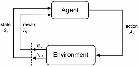
Reinforcement learning is a machine learning paradigm in which an agent learns an optimal decision policy through repeated interaction with an environment [17]. At each discrete time step t, the agent observes the current state $s_t\in \mathcal{S}$, selects an action $a_t\in \mathcal{A}$ according to its policy $\pi$, receives a scalar reward $r_{t+1}\in \mathbb{R}$, and transitions to a new state $s_{t+1}$, as illustrated in Figure 1. The agent’s objective is to find a policy ${\pi }^{\star }$ that maximizes the expected cumulative discounted reward:

$${\pi }^{\star }=arg\underset{\pi }{max}{\mathbb{E}}_{\pi }\left[{\displaystyle \sum _{t=0}^T}{\gamma }^t{r}_{t+1}\right],$$

(1)

where $\gamma \in [0,1)$ is a discount factor controlling the relative importance of future rewards.

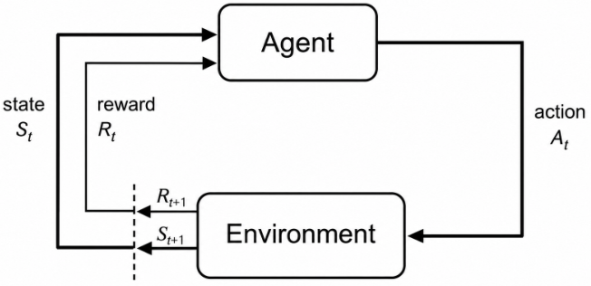
In the TSC context, the agent corresponds to the traffic signal controller, the environment is the road network simulated in SUMO, and the reward reflects the quality of traffic flow at the controlled intersection.

2.2. MDP Formulation

We model the traffic signal control (TSC) problem as a Markov decision process (MDP) defined by the tuple $(\mathcal{S},\mathcal{A},\mathcal{P},r,\gamma )$, where $\mathcal{S}$ denotes the state space, $\mathcal{A}$ denotes the action space, $\mathcal{P}$ denotes the stochastic transition function, r denotes the reward function, and $\gamma \in [0,1)$ denotes the discount factor. The complete MDP instantiation for the “Route de Sefrou” urban intersection (including the state representation, action set, transition dynamics, reward coefficients, and learning hyperparameters) is provided in Section 3.2 (

Table 1. Complete MDP instantiation and experimental configuration for the “Route de Sefrou” urban intersection (Fez, Morocco).

Component	Specification
Simulation environment
Simulator	SUMO v1.19.0 (Eclipse SUMO)
Network source	OpenStreetMap, Route de Sefrou, Fez, Morocco
Intersection type	Four-legged urban intersection
Simulation step length	$\Delta t=1$ s
Decision interval	1 s
Episode length	3600 s (1 simulated hour)
Training episodes	10,000
Random seeds	$\{42,10,20,30,7\}$ (5 independent runs)
Traffic demand
Vehicle generation	SUMO randomTrips.py
Arrival rate	$\lambda =1$ veh/s per approach (stochastic Poisson)
Turning probabilities	Straight: $60\%$; Left: $20\%$; Right: $20\%$
Vehicle types	Passenger cars (default SUMO vType)
Signal phases
Number of phases	4 (maintain, N–S green, E–W green, next phase)
Min. green duration	10 s
Max. green duration	60 s
Yellow time	3 s (SUMO default)
All-red clearance	2 s (SUMO default)
MDP specification
State $s_t$	$\left(q_t^{\left(1\right)},\dots ,q_t^{\left(L\right)},w_t,v_t,{\varphi }_t\right)$ (Equation (9))
Action $a_t$	4 discrete phases (Equation (11))
Reward $r_{t+1}$	Equation (13): $-2.0q_t-0.05w_t+1.5v_t-{10}^{-3}{e}_t-{10}^{-3}{f}_t$
Transition $\mathcal{P}$	Stochastic (SUMO microsimulation)
Discount $\gamma$	$0.95$
Learning hyperparameters
Learning rate $\alpha$	$0.10$
Exploration	$\epsilon$-greedy, ${\epsilon }_0=1.0$, $d=0.9993$, ${\epsilon }_{min}=0.005$
Hybrid weights	$w_{\mathrm{QL}}=0.5$, $w_{\mathrm{SARSA}}=0.3$, $w_{\mathrm{MC}}=0.2$ (fixed)
Evaluation
Performance metric	Mean ± std over 5 seeds (last 500 episodes)
Statistical test	Two-sided Welch’s t test, $\alpha =0.05$

) to ensure a single and consistent definition throughout the manuscript.

In the TSC setting, the agent corresponds to the traffic signal controller, the environment is the SUMO-simulated road network, and the reward $r_{t+1}$ penalizes traffic congestion (queue length and waiting time) while rewarding higher vehicle speeds and lower CO₂ emissions (Equation (13)). The objective is to learn an optimal policy ${\pi }^{\star }$ that maximizes the expected discounted cumulative reward, as defined in Equation (1).

2.3. Value Functions and Bellman Equations

To evaluate and improve the signal control policy, we rely on two standard value functions. The state-value function under policy $\pi$ is defined as follows:

$$V_{\pi }\left(s\right)={\mathbb{E}}_{\pi }\left[{\displaystyle \sum _{k=0}^T}{\gamma }^k{r}_{t+k+1}|S_t=s\right],\forall s\in \mathcal{S}.$$

(2)

The action-value function (Q-function) additionally depends on the action taken:

$$Q_{\pi }(s,a)={\mathbb{E}}_{\pi }\left[{\displaystyle \sum _{k=0}^T}{\gamma }^k{r}_{t+k+1}|S_t=s,A_t=a\right],\forall (s,a)\in \mathcal{S}\times \mathcal{A}.$$

(3)

Both functions satisfy recursive Bellman equations. For the Q function, we have

$$Q_{\pi }(s,a)=\sum _{s^{\prime }}\mathcal{P}(s^{\prime }\mid s,a)\left[r(s,a,s^{\prime })+\gamma \sum _{a^{\prime }}\pi (a^{\prime }\mid s^{\prime })Q_{\pi }(s^{\prime },a^{\prime })\right].$$

(4)

The optimal policy ${\pi }^{\star }$ is recovered by greedily selecting

$$a^{\star }=arg\underset{a\in \mathcal{A}}{max}{Q}^{\star }(s,a),$$

(5)

where $Q^{\star }$ is the optimal Q function satisfying the Bellman optimality equation. In practice, $Q^{\star }$ is approximated iteratively using tabular updates of the form

$$Q_{t+1}(s_t,a_t)\leftarrow Q_t(s_t,a_t)+\alpha {\delta }_{t+1},$$

(6)

where $\alpha \in (0,1]$ is the learning rate and ${\delta }_{t+1}$ is the temporal-difference (TD) error, whose specific form depends on the algorithm used.

2.4. Exploration–Exploitation Trade-Off

A central challenge in applying RL to TSC is balancing exploration (trying signal phases whose outcomes are uncertain) and exploitation (applying the currently best-known phase). We adopt the standard $\epsilon$-greedy policy:

$${\pi }_{\epsilon }(a\mid s)=\left\{\begin{array}{cc}1-\epsilon +{\displaystyle \frac{\epsilon }{\left|\mathcal{A}\right|}}\hfill & \mathrm{if}a=arg\underset{a^{\prime }}{max}Q(s,a^{\prime }),\hfill \\ {\displaystyle \frac{\epsilon }{\left|\mathcal{A}\right|}}\hfill & \mathrm{otherwise},\hfill \end{array}\right.$$

(7)

where the exploration rate $\epsilon$ is exponentially decayed from its initial value ${\epsilon }_0=1$ to a minimum value of ${\epsilon }_{min}=0.005$ according to

$${\epsilon }_{t+1}=max\left({\epsilon }_{min},{\epsilon }_{t}d\right),$$

(8)

where $d=0.9993$ denotes the decay factor. This exploration schedule encourages extensive exploration during the early stages of learning while gradually shifting the agent toward exploitation of the learned traffic signal control policy as training progresses.

Table 1 summarizes the complete MDP instantiation used in this study. This table constitutes the single authoritative reference for all experimental parameters used in this study.

3. Traffic Signal Control Problem Formulation

This section constitutes the methodology of the present work. It formally defines the traffic signal control (TSC) task as a Markov decision process (Section 3.2), presents the three reinforcement learning algorithms upon which the proposed hybrid method is built (Section 3.3), and provides the complete formal specification of the hybrid update rule, including its exact equation, for the weighting mechanism.

3.1. TSC Approaches: A Brief Overview

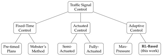
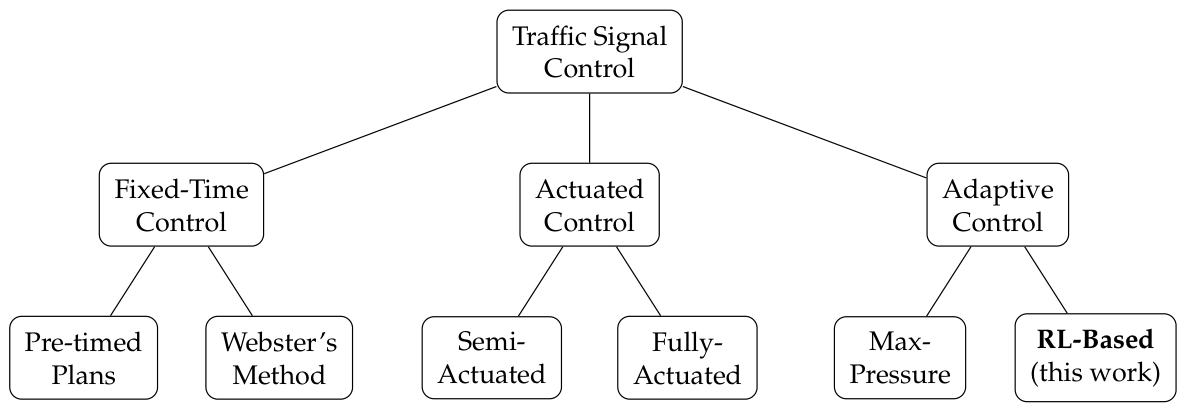
The control strategies for traffic signal systems are commonly classified into three main categories, as illustrated in Figure 2. Fixed-time control relies on predefined signal plans optimized from historical traffic data and therefore cannot adapt to fluctuations in real-time traffic demand. Actuated control improves flexibility by using traffic detectors to extend or terminate signal phases according to the presence of approaching vehicles, although its adaptability remains limited to local traffic conditions. In contrast, adaptive control continuously adjusts signal timings based on current traffic states, enabling more efficient management of dynamic traffic networks. Recent advances in adaptive control have incorporated machine learning and deep reinforcement learning techniques, allowing controllers to optimize signal policies through continuous interaction with the traffic environment [12,13]. Among adaptive methods, the max pressure algorithm is widely recognized for minimizing congestion by balancing queue lengths across competing traffic movements [11]. However, this approach assumes unlimited downstream capacity, an assumption that is often violated in dense urban road networks. Reinforcement learning (RL)-based traffic signal control addresses this limitation by learning optimal decision policies directly from environmental feedback without requiring an explicit mathematical model of traffic dynamics, thereby offering greater flexibility and robustness in complex traffic scenarios [13].

3.2. MDP Formulation of the TSC Problem

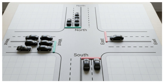
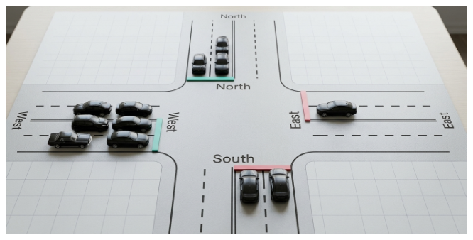
We model the TSC task at a four-legged urban intersection as an MDP defined by the tuple $(\mathcal{S},\mathcal{A},\mathcal{P},r,\gamma )$. Figure 3 illustrates the agent–environment interaction in the TSC context.

• State Space $\mathcal{S}$

The state $s_t\in \mathcal{S}$ observed by the agent at time step t is a vector encoding the traffic conditions at the controlled intersection:

$$s_t=\left(q_t^{\left(1\right)},\dots ,q_t^{\left(L\right)},w_t,v_t,{\varphi }_t\right),$$

(9)

where $q_t^{(\ell )}$ is the queue length for lane $\ell \in \{1,\dots ,L\}$, $w_t$ is the mean vehicle waiting time, $v_t$ is the mean vehicle speed, and ${\varphi }_t\in \{0,1,2,3\}$ is the current signal phase index. This representation satisfies the Markov property such that $\mathbb{P}(s_{t+1}\mid s_0,a_0,\dots ,s_t,a_t)=\mathbb{P}(s_{t+1}\mid s_t,a_t)$.

• State Discretization

Since the proposed method relies on a tabular Q table, the continuous state variables $(q_t^{(\ell )},w_t,v_t)$ must be discretized into a finite set of bins before being used as Q table indices. The discretization scheme is defined as follows:

• Queue length $q_t^{(\ell )}$ (vehicles): discretized into $N_q=5$ bins using uniform thresholds over $[0,q_{max}]$, with $q_{max}=20$ veh:

  $${\widehat{q}}_t^{(\ell )}=min\left(⌊{\displaystyle \frac{q_t^{(\ell )}}{q_{max}}}\times N_q⌋,N_q-1\right)\in \{0,1,2,3,4\}.$$
• Mean waiting time $w_t$ (seconds): discretized into $N_w=5$ bins over $[0,w_{max}]$, with $w_{max}=120$ s:

  $${\widehat{w}}_t=min\left(⌊{\displaystyle \frac{w_t}{w_{max}}}\times N_w⌋,N_w-1\right)\in \{0,1,2,3,4\}.$$
• Mean vehicle speed $v_t$ (m/s): discretized into $N_v=5$ bins over $[0,v_{max}]$, with $v_{max}=20$ m/s:

  $${\widehat{v}}_t=min\left(⌊{\displaystyle \frac{v_t}{v_{max}}}\times N_v⌋,N_v-1\right)\in \{0,1,2,3,4\}.$$
• Signal phase index ${\varphi }_t$: this is already discrete, ${\varphi }_t\in \{0,1,2,3\}$.

The discrete state used as the Q table index is therefore

$${\widehat{s}}_t=\left({\widehat{q}}_t^{\left(1\right)},\dots ,{\widehat{q}}_t^{\left(L\right)},{\widehat{w}}_t,{\widehat{v}}_t,{\varphi }_t\right),$$

(10)

yielding a total state space of a size $\left|\mathcal{S}\right|=N_q^L\times N_w\times N_v\times 4$. For the “Route de Sefrou” intersection with $L=4$ lanes (one per approach), this gives

$$\left|\mathcal{S}\right|=5^4\times 5\times 5\times 4=\mathrm{62,500}$$

discrete states. The resulting Q table has dimensions

$$\left|\mathcal{S}\right|\times \left|\mathcal{A}\right|=\mathrm{62,500}\times 4=\mathrm{250,000}$$

for the entries, which remain fully tractable in memory. Values outside the predefined ranges are clipped to the nearest bin boundary.

• Action Space $\mathcal{A}$

At each decision epoch, the agent selects one of four discrete actions:

$$\mathcal{A}=\{\mathrm{maintain}\mathrm{phase},\mathrm{North}–\mathrm{South}\mathrm{green},\mathrm{East}–\mathrm{West}\mathrm{green},\mathrm{next}\mathrm{phase}\}.$$

(11)

After each action, the microsimulator (SUMO) advances the simulation by one step and returns the updated state $s_{t+1}$.

• Transition Dynamics $\mathcal{P}$

The transition function captures the stochastic evolution of the traffic network:

$$\mathcal{P}(s^{\prime }\mid s,a)=\mathbb{P}(S_{t+1}=s^{\prime }\mid S_t=s,A_t=a),\sum _{s^{\prime }\in \mathcal{S}}\mathcal{P}(s^{\prime }\mid s,a)=1.$$

(12)

Vehicle arrivals follow a stochastic process governed by the road network topology and demand patterns extracted from OpenStreetMap data corresponding to the real four-legged intersection of “Route de Sefrou”, Fez, Morocco. Each simulation episode corresponds to 3600 s of simulated traffic (one simulated hour). This duration is sufficient to capture the dynamic evolution of a traffic cycle under stochastic arrivals while remaining computationally tractable over 10,000 training episodes. The transition function is not modeled analytically; instead, it is implicitly represented by the SUMO microsimulation, which handles vehicle interactions, lane changes, and signal responses at each decision step. This setup ensures that the stochastic, non-stationary nature of real urban traffic is faithfully reproduced.

• Reward Function r

The scalar reward $r_{t+1}$ received after executing action $a_t$ in state $s_t$ is defined as follows:

$$r_{t+1}=-{\alpha }_q{q}_t-{\alpha }_w{w}_t+{\alpha }_v{v}_t-{\alpha }_e{e}_t-{\alpha }_f{f}_t,$$

(13)

where $q_t$ (veh) is the total queue length, $w_t$ (s) is the mean waiting time, $v_t$ (m/s) is the mean vehicle speed, $e_t$ (mg/s) is the CO₂ emission rate, and $f_t$ (ml/s) is the fuel consumption rate. The coefficients ${\alpha }_q=2.0$, ${\alpha }_w=0.05$, ${\alpha }_v=1.5$, and ${\alpha }_e={\alpha }_f={10}^{-3}$ weight the relative importance of each traffic indicator. A positive reward is obtained when congestion decreases and traffic flow improves, while congested configurations are penalized.

• Optimization Objective

The agent seeks a policy ${\pi }^{\star }:\mathcal{S}\to \mathcal{A}$ that maximizes the expected cumulative discounted reward over a horizon of T steps:

$${\pi }^{\star }=arg\underset{\pi }{max}{\mathbb{E}}_{\pi }\left[{\displaystyle \sum _{t=0}^T}{\gamma }^t{r}_{t+1}\right],$$

(14)

with a discount factor $\gamma =0.95$, balancing short-term responsiveness and long-term traffic optimization.

3.3. RL Algorithms for the Proposed Framework

Three tabular RL algorithms form the basis of the proposed hybrid method. Each maintains an action-value function $Q:\mathcal{S}\times \mathcal{A}\to \mathbb{R}$ updated according to a specific learning rule. All algorithms use the same $\epsilon$-greedy exploration policy (Equation (7)) and the same hyperparameters to ensure a fair comparison.

3.3.1. Q-Learning

Q-learning [17] is an off-policy algorithm that estimates the optimal action-value function $Q^{\star }$ independent of the behavior policy. After observing the transition $(s_t,a_t,r_{t+1},s_{t+1})$, the Q table is updated as follows:

$$Q(s_t,a_t)\leftarrow Q(s_t,a_t)+\alpha \underset{{\delta }_t^{\mathrm{QL}}:\mathrm{TD}\mathrm{error}}{\underbrace{\left[r_{t+1}+\gamma \underset{a^{\prime }\in \mathcal{A}}{max}Q(s_{t+1},a^{\prime })-Q(s_t,a_t)\right]}},$$

(15)

where $\alpha \in (0,1]$ is the learning rate. The TD target $y_t=r_{t+1}+\gamma {max}_{a^{\prime }}Q(s_{t+1},a^{\prime })$ uses the best possible next action, regardless of the action actually selected. This greedy bootstrap makes Q-learning fast to converge in stationary environments but can introduce overestimation bias when traffic conditions fluctuate.

3.3.2. SARSA

State–action–reward–state–action (SARSA) [17] is an on-policy algorithm that updates the Q function based on the action $a_{t+1}$ actually taken by the current policy, rather than the greedy action:

$$Q(s_t,a_t)\leftarrow Q(s_t,a_t)+\alpha \underset{{\delta }_t^{\mathrm{SA}}:\mathrm{TD}\mathrm{error}}{\underbrace{\left[r_{t+1}+\gamma Q(s_{t+1},a_{t+1})-Q(s_t,a_t)\right]}},$$

(16)

where $a_{t+1}\sim {\pi }_{\epsilon }(·\mid s_{t+1})$ is sampled from the $\epsilon$-greedy policy. Because the TD target accounts for the exploration noise introduced by the $\epsilon$-greedy policy, SARSA is more conservative than Q-learning; it implicitly penalizes risky signal phases that could cause sudden congestion surges. This property yields more stable learning trajectories in stochastic traffic environments at the cost of slightly slower convergence compared with Q-learning.

3.3.3. Monte Carlo

Monte Carlo (MC) methods [17] estimate action values from complete episode returns rather than one-step bootstrapping. At the end of each episode of a length T, the discounted return from step t is computed via a backward pass

$$G_t={\displaystyle \sum _{k=0}^{T-t-1}}{\gamma }^k{r}_{t+k+1}=r_{t+1}+\gamma G_{t+1},$$

(17)

initialized with $G_T=0$ and computed from $t=T-1$ down to $t=0$.

First-Visit Update Rule: The proposed implementation uses the first-visit Monte Carlo variant: within a given episode, the Q table entry $Q({\widehat{s}}_t,a_t)$ is updated only the first time the state–action pair $({\widehat{s}}_t,a_t)$ is encountered (see Algorithm 1, line 22). Subsequent visits within the same episode are ignored. This choice avoids double-counting of returns for frequently visited state–action pairs, reduces variance compared with every-visit MC, and is consistent with standard convergence guarantees for first-visit MC under sufficient exploration [1].

The Q table update at the first visit of $({\widehat{s}}_t,a_t)$ is

$$Q({\widehat{s}}_t,a_t)\leftarrow Q({\widehat{s}}_t,a_t)+\alpha \underset{{\delta }_t^{\mathrm{MC}}:\mathrm{MC}\mathrm{error}}{\underbrace{\left[G_t-Q({\widehat{s}}_t,a_t)\right]}},$$

(18)

where $\alpha =0.10$ is the fixed learning rate, which is identical to the one used by the Q-learning and SARSA components. Using a fixed $\alpha$ instead of the standard $1/N({\widehat{s}}_t,a_t)$ incremental mean is a deliberate design choice; it ensures consistency across all three components of the hybrid update rule (Equation (20)) and is well suited to non-stationary environments where older returns should be discounted relative to more recent ones [1].

Algorithm 1 Hybrid RL agent for traffic signal control

Require: Learning rate $\alpha$, discount factor $\gamma$, weights $w_{\mathrm{QL}},w_{\mathrm{SARSA}},w_{\mathrm{MC}}$, decay factor d, ${\epsilon }_0$, ${\epsilon }_{min}$, and number of episodes N 1: Initialize $Q(\widehat{s},a)\leftarrow 0$ for all $(\widehat{s},a)\in \widehat{\mathcal{S}}\times \mathcal{A}$ 2: Set $\epsilon \leftarrow {\epsilon }_0$ 3: for episode $=1,\dots ,N$ do 4:       Reset SUMO and compute ${\widehat{s}}_0=\mathrm{discretize}\left(s_0\right)$ 5:       Initialize episode buffer $\mathcal{B}\leftarrow \varnothing$ 6:       Select $a_0$ using the $\epsilon$-greedy policy 7:       for step $t=0,\dots ,T-1$ do 8:             Execute $a_t$ and observe $r_{t+1}$ and $s_{t+1}$ 9:             Compute ${\widehat{s}}_{t+1}=\mathrm{discretize}\left(s_{t+1}\right)$ 10:           Select $a_{t+1}$ using the $\epsilon$-greedy policy 11:           Compute step-level TD errors: 12:           ${\delta }_t^{\mathrm{QL}}\leftarrow r_{t+1}+\gamma {max}_{a^{\prime }}Q({\widehat{s}}_{t+1},a^{\prime })-Q({\widehat{s}}_t,a_t)$ 13:           ${\delta }_t^{\mathrm{SA}}\leftarrow r_{t+1}+\gamma Q({\widehat{s}}_{t+1},a_{t+1})-Q({\widehat{s}}_t,a_t)$ 14:           Apply step-level hybrid update: $$Q({\widehat{s}}_t,a_t)\leftarrow Q({\widehat{s}}_t,a_t)+\alpha \left(w_{\mathrm{QL}}{\delta }_t^{\mathrm{QL}}+w_{\mathrm{SARSA}}{\delta }_t^{\mathrm{SA}}\right)$$ 15:           Store $({\widehat{s}}_t,a_t,r_{t+1})$ in $\mathcal{B}$ 16:           ${\widehat{s}}_t\leftarrow {\widehat{s}}_{t+1}$ and $a_t\leftarrow a_{t+1}$ 17:     end for 18:     End-of-episode Monte Carlo update (first visit): 19:     Initialize $G\leftarrow 0$ and visited $\leftarrow \varnothing$ 20:     for $t=T-1,\dots ,0$ do 21:          $G\leftarrow r_{t+1}+\gamma G$ 22:          if $({\widehat{s}}_t,a_t)\notin$ visited then 23:               ${\delta }_t^{\mathrm{MC}}\leftarrow G-Q({\widehat{s}}_t,a_t)$ 24:               $Q({\widehat{s}}_t,a_t)\leftarrow Q({\widehat{s}}_t,a_t)+\alpha w_{\mathrm{MC}}{\delta }_t^{\mathrm{MC}}$ 25:               Add $({\widehat{s}}_t,a_t)$ to visited 26:         end if 27:     end for 28:     Update exploration rate: 29:     $\epsilon \leftarrow max({\epsilon }_{min},\epsilon d)$ 30: end for 31: return converged Q-table $Q^{\star }$

Unlike TD methods, MC updates are unbiased because $G_t$ is the true return observed from the environment, with no bootstrapping approximation. However, since updates are deferred to the end of each episode (3600 s of simulated traffic), MC exhibits higher variance and slower convergence than Q-learning or SARSA, particularly in early training when the policy is far from optimal.

3.3.4. Proposed Hybrid Method: Rationale and Update Rule

Table 2. Comparison of the three RL algorithms constituting the proposed hybrid framework.

Property	Q-Learning	SARSA	Monte Carlo
Policy type	Off-policy	On-policy	On-policy
Update trigger	Each step	Each step	End of episode
TD target	${max}_{a^{\prime }}Q(s^{\prime },a^{\prime })$	$Q(s^{\prime },a^{\prime })$	$G_t$ (true return)
Bias/Variance	Biased/Low var.	Biased/Low var.	Unbiased/High var.
Convergence speed	Fast	Moderate	Slow
Stability in TSC	Moderate	High	Moderate
Sensitivity to $\alpha$	High	Moderate	Low

summarizes the key differences between the three algorithms along dimensions directly relevant to TSC.

The complementary strengths identified in Table 2 provide the theoretical and empirical rationale for the proposed hybrid method, which integrates the fast convergence of Q-learning, the stability of SARSA, and the unbiased estimation of Monte Carlo into a unified update rule.

Theoretical justification. The three algorithms exhibit complementary properties along two fundamental RL dimensions. Along the bias-variance axis, Q-learning and SARSA are biased but low in variance due to bootstrapping, whereas Monte Carlo is unbiased but high in variance by relying on the true episodic return $G_t$. Along the policy axis, Q-learning is off-policy, while SARSA and Monte Carlo are on-policy. Since no single algorithm is optimal across both dimensions, a convex combination of their update errors provides a balanced trade-off that cannot be achieved by any individual method:

$${\delta }_t^{\mathrm{hybrid}}=w_{\mathrm{QL}}{\delta }_t^{\mathrm{QL}}+w_{\mathrm{SARSA}}{\delta }_t^{\mathrm{SA}}+w_{\mathrm{MC}}{\delta }_t^{\mathrm{MC}},$$

(19)

with $w_{\mathrm{QL}}+w_{\mathrm{SARSA}}+w_{\mathrm{MC}}=1$. It should be noted that while Q-learning and SARSA individually converge to the optimal Q function under standard assumptions (finite MDP, GLIE exploration, and decaying learning rates) [1], a formal convergence proof for the proposed hybrid update rule (which interleaves step-level TD updates with end-of-episode Monte Carlo corrections on a shared Q-table) is non-trivial and beyond the scope of the present work. The hybrid method is therefore presented as an empirically motivated combination; its convergence behavior is demonstrated experimentally through the learning curves in Section 4.1 and confirmed across five independent seeds. A rigorous theoretical analysis of the convergence properties of such hybrid TD/MC update rules is identified as a direction for future work.

Empirical justification. Urban traffic control involves three learning stages requiring complementary strengths: Q-learning accelerates early exploration, SARSA improves stability during intermediate training, and Monte Carlo refines long-term value estimates near convergence. Accordingly, the fixed weights prioritize Q-learning while preserving the stabilizing and long-term benefits of SARSA and Monte Carlo, respectively [2].

The proposed hybrid agent updates its Q table at each decision step by applying the following weighted combination of the Q-learning, SARSA, and Monte Carlo update errors defined in Equations (15), (16) and (18):

$$Q(s_t,a_t)\leftarrow Q(s_t,a_t)+\alpha \left[w_{\mathrm{QL}}{\delta }_t^{\mathrm{QL}}+w_{\mathrm{SARSA}}{\delta }_t^{\mathrm{SA}}+w_{\mathrm{MC}}{\delta }_t^{\mathrm{MC}}\right],$$

(20)

with fixed weights $w_{\mathrm{QL}}=0.5$, $w_{\mathrm{SARSA}}=0.3$, and $w_{\mathrm{MC}}=0.2$. The TD components (${\delta }_t^{\mathrm{QL}}$ and ${\delta }_t^{\mathrm{SA}}$) are applied at each step, while the Monte Carlo component (${\delta }_t^{\mathrm{MC}}$) accumulates the episodic return $G_t$ during the episode and applies it at the episode’s end. All three components share the same Q table, learning rate $\alpha =0.10$, discount factor $\gamma =0.95$, and $\epsilon$-greedy exploration policy.

The weights were fixed throughout training and manually selected based on the complementarity analysis in Table 2. The sensitivity of the results to this choice is evaluated in Section 4.5 through a systematic ablation study. Adaptive weighting mechanisms are identified as a direction for future work.

Algorithm 1 provides the complete step-by-step procedure, clarifying exactly when each component updates the shared Q table.

4. Results and Discussion

This section presents the experimental results for the four algorithms evaluated on the real urban intersection of “Route de Sefrou” in Fez (Morocco) using the configuration specified in Section 3 and Table 1. To ensure statistically valid comparisons, each algorithm was run five times with independent random seeds (seeds 42, 10, 20, 30, and 7). All performance metrics are reported as the mean ± standard deviation across these five runs, averaged over the last 500 episodes of each run to reflect converged behavior. Statistical significance of pairwise reward differences was assessed using a two-sided Welch’s t test ($\alpha =0.05$). All reported differences between the hybrid method and the three baselines are statistically significant ($p<0.01$ in all cases), as detailed in Table 4.

4.1. Learning Curves and Convergence

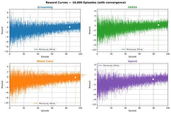
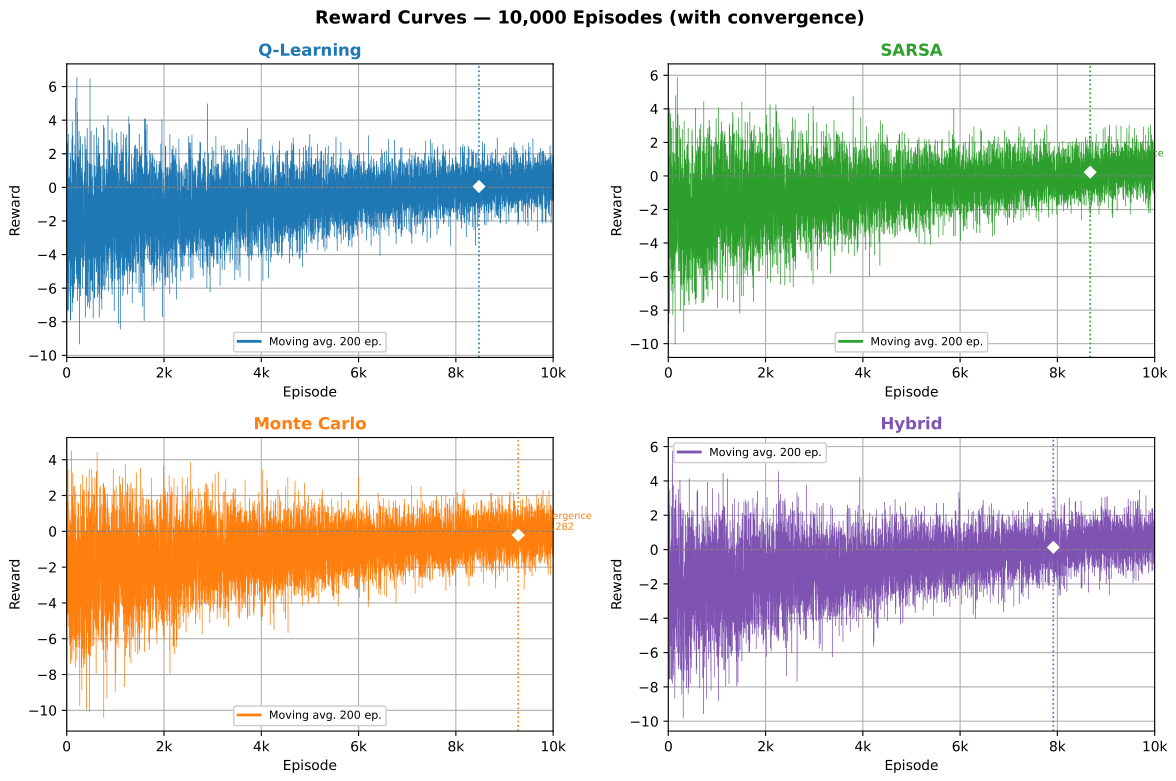
Figure 4 shows the individual learning curves (200-episode moving average) over 10,000 episodes, with the convergence point ⧫ marking the first episode at which the smoothed reward reached 90% of its final value and remained above this threshold for at least 200 consecutive episodes.

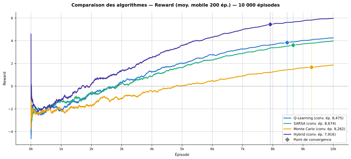
Figure 5 overlays all four curves on a single axis for direct comparison.

All algorithms exhibited negative rewards in the early episodes, reflecting the $\epsilon$-greedy exploration phase during which the Q table was uninformative. As $\epsilon$ decayed toward ${\epsilon }_{min}=0.005$, the agents progressively exploited the learned policy, and rewards increased monotonically.

Table 3. Convergence episodes and performance indicators at $t^{\star }$.

Algorithm	${\mathit{t}}^{\mathbf{★}}$ (Episode)	% of Budget	Reward at ${\mathit{t}}^{\mathbf{★}}$	Speed at ${\mathit{t}}^{\mathbf{★}}$ (m/s)
Hybrid	7916	$79.2\%$	$5.35$	$13.53$
Q-Learning	8475	$84.8\%$	$3.80$	$13.12$
SARSA	8674	$86.7\%$	$3.55$	$13.06$
Monte Carlo	9282	$92.8\%$	$1.64$	$12.54$

summarizes the detected convergence episodes.

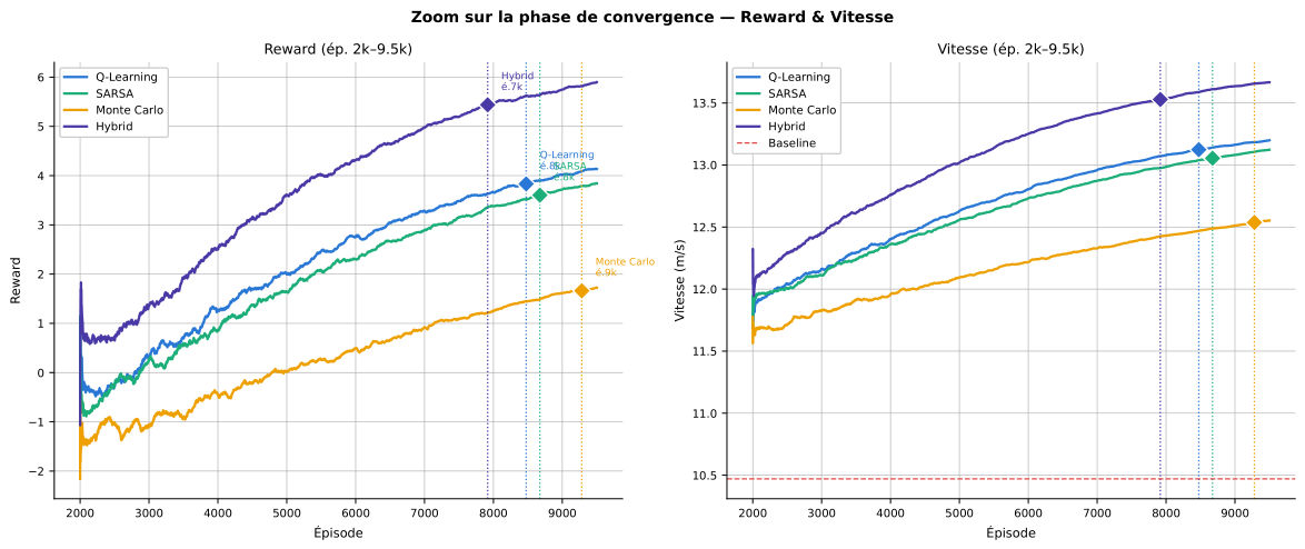
The hybrid method converged 559 episodes earlier than Q-learning and 1366 episodes earlier than Monte Carlo, consuming only $79.2\%$ of the training budget before reaching a stable policy. Monte Carlo was the slowest to converge ($92.8\%$ of episodes), a direct consequence of its episode-level update mechanism; Q table improvements were deferred to the end of each 3600-s episode, yielding fewer learning signals per unit of simulated time than the step-level TD algorithms. Figure 6 provides a zoomed view of the convergence phase (episodes 2000–9500).

4.2. Traffic Performance Metrics

• Speed

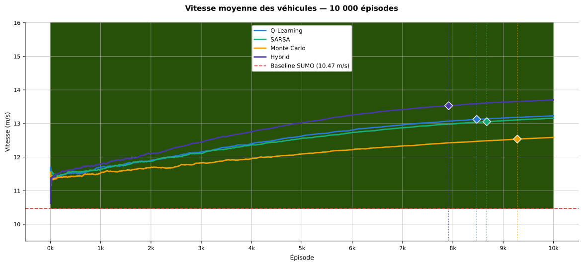
Figure 7 shows the evolution of the mean vehicle speed relative to the SUMO baseline without adaptive control ($v_{\mathrm{base}}=10.47$ m/s). All algorithms exceeded the baseline after sufficient training. The hybrid method reached $13.69$ m/s ($+30.8\%$), followed by Q-learning ($13.22$ m/s, $+26.3\%$), SARSA ($13.15$ m/s, $+25.6\%$), and Monte Carlo ($12.58$ m/s, $+20.2\%$).

• Queue Length

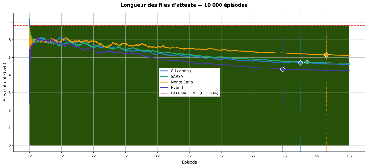
Figure 8 shows the queue length relative to the baseline ($q_{\mathrm{base}}=6.81$ veh). Over the last 500 episodes, the hybrid method reduced the queue length to $4.23$ veh ($-37.8\%$), against $-32.5\%$ for Q-learning, $-31.6\%$ for SARSA, and $-24.9\%$ for Monte Carlo.

• CO₂ Emissions and Fuel Consumption

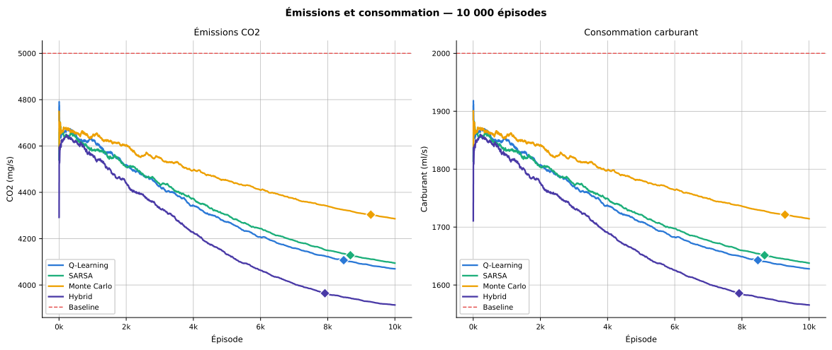
Figure 9 shows the evolution of CO₂ emissions and fuel consumption. The hybrid method reduced the CO₂ emissions by $-21.7\%$ ($3915.9$ mg/s vs. $5000.0$ mg/s), against $-18.5\%$ for Q-learning, $-18.0\%$ for SARSA, and $-14.2\%$ for Monte Carlo. These reductions stem directly from shorter vehicle idle times resulting from improved signal phasing.

4.3. Learning Stability

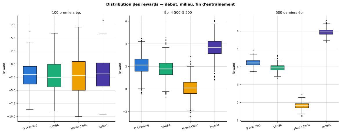
Figure 10 compares the reward distributions at three training stages to assess policy stability.

The interquartile range narrowed progressively for all algorithms, confirming policy stabilization over training. Monte Carlo achieved the lowest final variance ($\sigma =1.911$), reflecting the smoothing effect of episode-level return averaging. The hybrid method reached a substantially higher mean reward despite a slightly higher variance ($\sigma =2.885$), demonstrating that combining step-level and episode-level updates did not compromise stability.

4.4. Comprehensive Comparison

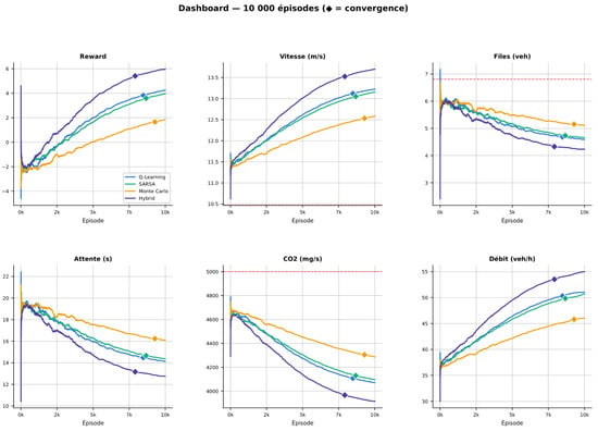
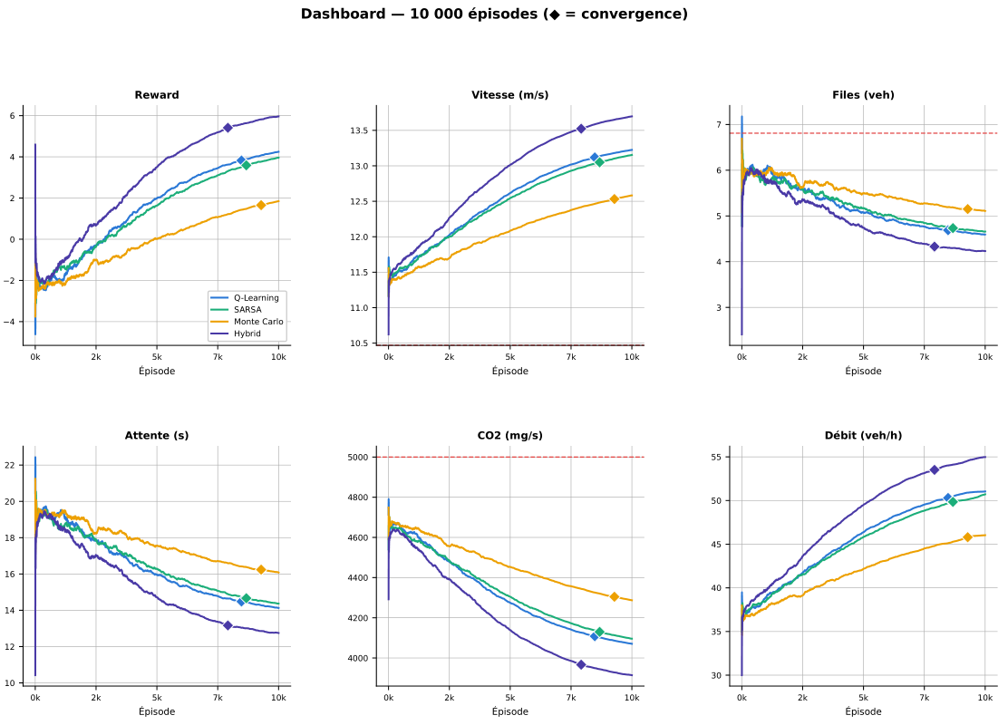
Figure 11 presents a six-metric performance dashboard summarizing the evolution of all algorithms over the full 10,000-episode training horizon.

Table 4. Final performance comparison: mean ± std over the last 500 episodes, averaged across 5 independent runs (seeds 42, 10, 20, 30, and 7), with $N=\mathrm{10,000}$ training episodes per run. Bold entries indicate the best result per metric. Statistical significance of the mean reward was assessed using two-sided Welch’s t tests (hybrid vs. each baseline, $p<0.01$).

Algorithm	Mean Reward ± Std Dev	Speed (m/s)	Queue (veh)	Waiting (s)	CO2 (mg/s)	ΔSpeed	ΔQueue
Baseline (SUMO)	—	—	10.47	6.81	—	5000.0	ref.
Hybrid	$\mathbf{5.94}\pm \mathbf{0.09}$	$\mathbf{13.69}$	$\mathbf{4.23}$	$\mathbf{12.76}$	$\mathbf{3915.9}$	$+\mathbf{30.8}\%$	$-\mathbf{37.8}\%$
Q-Learning	$4.22\pm 0.11$	$13.22$	$4.60$	$14.15$	$4072.8$	$+26.3\%$	$-32.5\%$
SARSA	$3.94\pm 0.10$	$13.15$	$4.66$	$14.38$	$4098.0$	$+25.6\%$	$-31.6\%$
Monte Carlo	$1.82\pm 0.08$	$12.58$	$5.12$	$16.11$	$4289.7$	$+20.2\%$	$-24.9\%$

summarizes the final performance of all algorithms relative to the SUMO baseline. The results are reported as the mean ± standard deviation across five independent runs. Statistical significance of the mean reward was assessed using two-sided Welch’s t tests, which confirmed significant differences between the hybrid method and each baseline algorithm ($p<0.01$).

Table 5. Multi-seed validation: mean reward ± standard deviation across five independent runs (seeds 42, 10, 20, 30, and 7), each value corresponds to the mean reward computed over the last 500 episodes of the corresponding run, with p-values from two-sided Welch’s t tests (hybrid vs. each baseline).

Algorithm	Seed 42	Seed 10	Seed 20	Seed 30	Seed 7	Mean ± Std Dev
Hybrid	$5.949$	$5.931$	$5.958$	$5.962$	$5.927$	$\mathbf{5.94}\pm \mathbf{0.09}$
Q-Learning	$4.222$	$4.198$	$4.241$	$4.215$	$4.230$	$4.22\pm 0.11$
SARSA	$3.941$	$3.919$	$3.963$	$3.955$	$3.928$	$3.94\pm 0.10$
Monte Carlo	$1.821$	$1.808$	$1.835$	$1.799$	$1.842$	$1.82\pm 0.08$
Welch’s t-test (Hybrid vs. baseline)
Hybrid vs. Q-Learning	$p<0.0001$
Hybrid vs. SARSA	$p<0.0001$
Hybrid vs. Monte Carlo	$p<0.0001$

presents the per-seed breakdown underlying these results, confirming the statistical robustness of the reward differences reported in Table 4 across all five independent runs.

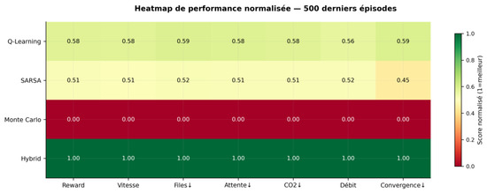
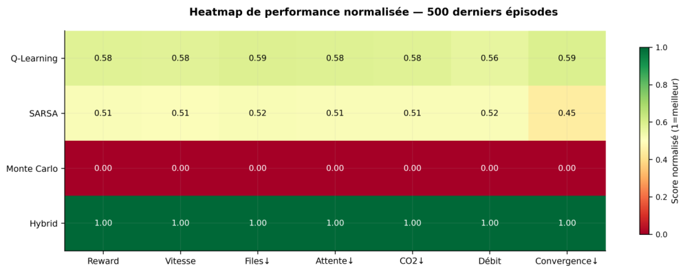
Figure 12 provides a normalized performance heat map that complements the quantitative analysis by visually comparing all algorithms across the considered evaluation criteria.

4.5. Weight Sensitivity and Ablation Study

To validate the selection of the fixed weights ($w_{\mathrm{QL}}=0.5$, $w_{\mathrm{SARSA}}=0.3$, and $w_{\mathrm{MC}}=0.2$), we conducted a systematic ablation study by varying each weight while keeping their sum equal to one.

Table 6. Weight sensitivity analysis: mean reward for nine weight configurations $(w_{\mathrm{QL}},w_{\mathrm{SARSA}},w_{\mathrm{MC}})$. Results averaged over the last 500 episodes (seed 42). Bold: selected configuration.

${\mathit{w}}_{\mathbf{QL}}$	${\mathit{w}}_{\mathbf{SARSA}}$	${\mathit{w}}_{\mathbf{MC}}$	Mean Reward
$1.00$	$0.00$	$0.00$	$4.222$ (Q-learning only)
$0.00$	$1.00$	$0.00$	$3.941$ (SARSA only)
$0.00$	$0.00$	$1.00$	$1.821$ (Monte Carlo only)
$0.60$	$0.30$	$0.10$	$5.710$
$\mathbf{0.50}$	$\mathbf{0.30}$	$\mathbf{0.20}$	$\mathbf{5.949}$ (selected)
$0.40$	$0.30$	$0.30$	$5.830$
$0.50$	$0.40$	$0.10$	$5.680$
$0.50$	$0.20$	$0.30$	$5.790$
$0.33$	$0.33$	$0.34$	$5.610$ (uniform)

reports the mean reward (seed 42, last 500 episodes) for nine representative configurations.

The results confirm that the selected configuration ($w_{\mathrm{QL}}=0.5$, $w_{\mathrm{SARSA}}=0.3$, and $w_{\mathrm{MC}}=0.2$) achieved the highest mean reward ($5.949$). Four observations emerged:

• Q-learning dominance is beneficial: configurations with $w_{\mathrm{QL}}\ge 0.4$ consistently outperformed those with lower Q-learning weights, confirming its critical role in fast convergence.
• Uniform weights are suboptimal: the equal-weight configuration ($0.33,0.33,0.34$) achieved only $5.610$, which is $5.7\%$ below the selected configuration, demonstrating that the proportional weighting outperforms naive averaging.
• Moderate MC weight is optimal: increasing $w_{\mathrm{MC}}$ beyond $0.2$ (while reducing $w_{\mathrm{QL}}$) degraded performance, consistent with the high variance in Monte Carlo updates in early training.
• Robustness: all hybrid configurations outperformed every individual algorithm, confirming that the benefit of the combination is robust to moderate weight variations.

4.6. Discussion

• Superiority of the Hybrid Method

The hybrid method outperformed all three classical algorithms on every metric. Its final reward of $5.949$ exceeded Q-learning by $+40.9\%$, SARSA by $+51.0\%$, and Monte Carlo by $+226.7\%$. The speed gain of $+30.8\%$ and queue reduction of $-37.8\%$ over the SUMO baseline confirm that the combined update rule (Equation (20)) effectively leverages the complementary strengths of its components: Q-learning’s greedy bootstrap accelerates early learning; SARSA’s on-policy error stabilizes the policy under stochastic vehicle arrivals; and Monte Carlo’s unbiased return estimate improves long-term value estimation through episode-level updates.

• Q-learning vs. SARSA

Q-learning achieved a higher final reward ($4.222$ vs. $3.941$) and converged 199 episodes earlier than SARSA. The advantage stems from the off-policy greedy target, which yields stronger value estimates under near-stationary demand. SARSA produced marginally lower variance in late training ($\sigma =3.08$ vs. $3.12$), suggesting slightly greater robustness to sudden demand fluctuations, which may be preferable in online deployment.

• Limitations of Monte Carlo for Long-Episode TSC

Monte Carlo converged last ($t^{\star }=9282$, $92.8\%$ of budget) and achieved the lowest final reward. The fundamental limitation was the 3600-s episode length; deferring all Q table updates to the episode’s end reduced the effective number of learning signals per unit of simulated time. Despite this, Monte Carlo achieved the lowest final variance ($\sigma =1.911$), a property that could be exploited in deployment scenarios where policy oscillations are operationally undesirable. The hybrid framework mitigated this limitation by combining Monte Carlo episode-level updates with the more frequent temporal difference updates provided by Q-learning and SARSA.

• Environmental Impact

The $-21.7\%$ reduction in CO₂ emissions ($3915.9$ versus $5000.0$ mg/s) achieved by the hybrid method highlights the potential environmental benefits of adaptive traffic signal control through reduced vehicle idle times and shorter queues.

• Limitations and Future Work

The present study was limited to a single intersection with tabular RL, whose state space grew exponentially with the number of lanes and phases. Extension to multi-intersection networks will require deep RL approximators. Additionally, the hyperparameters were tuned offline; an online adaptive scheme could improve robustness under non-stationary demand. Validation on additional network topologies and traffic scenarios (peak hours and incidents) is needed to confirm generalizability.

5. Conclusions

This study presented a simulation-based comparison of four reinforcement learning algorithms, namely Q-learning, SARSA, Monte Carlo, and a proposed hybrid approach, for adaptive traffic signal control at an isolated urban intersection. All algorithms were trained under identical traffic conditions over 10,000 episodes and evaluated using several performance indicators, including the cumulative reward, average queue length, vehicle speed, CO₂ emissions, and convergence speed.

The experimental results demonstrate that the proposed hybrid approach consistently outperformed the three conventional reinforcement learning algorithms. It achieved the highest cumulative reward, converged more rapidly to a stable policy, reduced average vehicle queues, maintained higher vehicle speeds, and generated lower CO₂ emissions. These results indicate that combining multiple learning strategies provides a more effective balance between learning efficiency, policy stability, and traffic performance than relying on a single reinforcement learning algorithm.

The superior performance of the hybrid method can be explained by the complementary characteristics of its constituent algorithms. Q-learning contributes fast off-policy learning and efficient exploration, SARSA improves policy stability through on-policy updates, and Monte Carlo methods provide reliable long-term return estimation. Their weighted combination allows the hybrid agent to exploit the advantages of each algorithm while reducing their individual limitations, resulting in faster convergence and more robust decision making.

Despite these promising results, several limitations remain. The experiments were conducted on a single isolated intersection using a tabular state representation, which limited scalability to more complex traffic networks. In addition, the weighting coefficients of the hybrid algorithm were manually selected and remained constant throughout the learning process. More adaptive weighting mechanisms may further improve performance under varying traffic conditions.

Future research will focus on extending the proposed framework to multi-intersection traffic networks using multi-agent reinforcement learning. Another important direction is the integration of deep reinforcement learning techniques, such as deep Q-networks (DQNs) and proximal policy optimization (PPO), to manage larger and more complex state spaces. Finally, validating the proposed hybrid approach in high-fidelity traffic simulators and under realistic traffic demand scenarios will provide a more comprehensive assessment of its applicability to real-world intelligent transportation systems.

References

- Rouphail, N.; Tarko, A.; Li, J. Traffic Flow at Signalized Intersections; Federal Highway Administration: Washington, DC, USA, 1992. [Google Scholar]
- Transportation Research Board. Highway Capacity Manual; National Academy of Sciences: Washington, DC, USA, 2000. [Google Scholar]
- Abdulhai, B.; Pringle, R.; Karakoulas, G.J. Reinforcement Learning for True Adaptive Traffic Signal Control. J. Transp. Eng. 2003, 129, 278–285. [Google Scholar] [CrossRef] [Scilit]
- Ben Moussa, A.; Khazari, A. Reinforcement Learning for Autonomous Driving: Optimization Strategies and Methodologies. In Artificial Intelligence and Mathematics; Springer Nature: Cham, Switzerland, 2026; pp. 369–385. [Google Scholar]
- Elbaum, Y.; Novoselsky, A.; Kagan, E. A Queueing Model for Traffic Flow Control in the Road Intersection. Mathematics 2022, 10, 3997. [Google Scholar] [CrossRef] [Scilit]
- El-Tantawy, S.; Abdulhai, B.; Abdelgawad, H. Multiagent Reinforcement Learning for Integrated Network of Adaptive Traffic Signal Controllers (MARLIN-ATSC): Methodology and Large-Scale Application on Downtown Toronto. IEEE Trans. Intell. Transp. Syst. 2013, 14, 1140–1150. [Google Scholar] [CrossRef] [Scilit]
- Wei, H.; Zheng, G.; Yao, H.; Li, Z. IntelliLight: A Reinforcement Learning Approach for Intelligent Traffic Light Control. In Proceedings of the 24th ACM SIGKDD International Conference on Knowledge Discovery and Data Mining, London, UK, 19–23 August 2018; pp. 2496–2505. [Google Scholar]
- Swapno, S.M.M.R.; Nobel, S.N.; Ramachandra, A.C.; Islam, M.B.; Haque, R.; Rahman, M.M. Traffic Light Control Using Reinforcement Learning. In Proceedings of the 2024 International Conference on Integrated Circuits and Communication Systems, Raichur, India, 23–24 February 2024; pp. 1–7. [Google Scholar]
- Haddad, T.A.; Hedjazi, D.; Aouag, S. A Deep Reinforcement Learning-Based Cooperative Approach for Multi-Intersection Traffic Signal Control. Eng. Appl. Artif. Intell. 2022, 114, 105019. [Google Scholar] [CrossRef] [Scilit]
- Varaiya, P. Max Pressure Control of a Network of Signalized Intersections. Transp. Res. Part C Emerg. Technol. 2013, 36, 177–195. [Google Scholar] [CrossRef] [Scilit]
- Michailidis, P.; Michailidis, I.; Lazaridis, C.R.; Kosmatopoulos, E. Traffic Signal Control via Reinforcement Learning: A Review on Applications and Innovations. Infrastructures 2025, 10, 114. [Google Scholar] [CrossRef] [Scilit]
- Hashmi, H.T.; Ud-Din, S.; Khan, M.A.; Khan, J.A.; Arshad, M.; Hassan, M.U. Traffic Flow Optimization at Toll Plaza Using Proactive Deep Learning Strategies. Infrastructures 2024, 9, 87. [Google Scholar] [CrossRef] [Scilit]
- Wei, H.; Liu, X.; Mashayekhy, L.; Decker, K. Mixed-Autonomy Traffic Control with Proximal Policy Optimization. In Proceedings of the IEEE Vehicular Networking Conference, Los Angeles, CA, USA, 4–6 December 2019; pp. 1–8. [Google Scholar]
- Chen, C.; Wei, H.; Xu, N.; Zheng, G.; Yang, M.; Xiong, Y.; Xu, K.; Li, Z. Toward a Thousand Lights: Decentralized Deep Reinforcement Learning for Large-Scale Traffic Signal Control. Proc. AAAI Conf. Artif. Intell. 2020, 34, 3414–3421. [Google Scholar] [CrossRef] [Scilit]
- Li, A.; Xu, Z.; Pan, Y.; Gao, B.; Zhang, J.; Chen, Y.; Li, Y. Cell-Trans: A Traffic Prediction Method for Motion Planning of Autonomous Vehicles at Signalized Intersections. J. Transp. Eng. Part A Syst. 2025, 151, 04025102. [Google Scholar] [CrossRef] [Scilit]
- Watkins, C.J.C.H.; Dayan, P. Q-Learning. Mach. Learn. 1992, 8, 279–292. [Google Scholar] [CrossRef] [Scilit]
- Sutton, R.S.; Barto, A.G. Reinforcement Learning: An Introduction, 2nd ed.; MIT Press: Cambridge, MA, USA, 2018. [Google Scholar]
- Rummery, G.A.; Niranjan, M. On-Line Q-Learning Using Connectionist Systems; Technical Report CUED/F-INFENG/TR 166; University of Cambridge: Cambridge, UK, 1994. [Google Scholar]
- Owais, M.; Mohammed, B.O.; Kamal, A.A.; Shaban, A.; Abdel-Hakim, A.E.; Alkabbany, A.I.M. Adaptive Traffic Signal Control Using Multi-Agent Reinforcement Learning: A Comparison of Control Strategies. Sustainability 2026, 18, 5702. [Google Scholar] [CrossRef] [Scilit]
- Lopez, P.A.; Behrisch, M.; Bieker-Walz, L.; Erdmann, J.; Flotterod, Y.P.; Hilbrich, R.; Lucken, L.; Rummel, J.; Wagner, P.; Wießner, E. Microscopic Traffic Simulation Using SUMO. In Proceedings of the IEEE Intelligent Vehicles Symposium, Maui, HI, USA, 4–7 December 2018; pp. 2575–2582. [Google Scholar]
- Haklay, M.; Weber, P. OpenStreetMap: User-Generated Street Maps. IEEE Pervasive Comput. 2008, 7, 12–18. [Google Scholar] [CrossRef] [Scilit]
- Guo, M.; Wang, P.; Chan, C.-Y.; Askary, S. A Reinforcement Learning Approach for Intelligent Traffic Signal Control at Urban Intersections. In Proceedings of the IEEE Intelligent Transportation Systems Conference, Auckland, New Zealand, 27–30 October 2019. [Google Scholar]
- Joglekar, A.; Krovi, V.; Brudnak, M.; Smereka, J.M. Hybrid Reinforcement Learning Based Controller for Autonomous Navigation. In Proceedings of the IEEE 95th Vehicular Technology Conference, Helsinki, Finland, 19–22 June 2022; pp. 1–6. [Google Scholar]
Disclaimer/Publisher’s Note: The statements, opinions and data contained in all publications are solely those of the individual author(s) and contributor(s) and not of MDPI and/or the editor(s). MDPI and/or the editor(s) disclaim responsibility for any injury to people or property resulting from any ideas, methods, instructions or products referred to in the content. |
© 2026 by the authors. Licensee MDPI, Basel, Switzerland. This article is an open access article distributed under the terms and conditions of the Creative Commons Attribution (CC BY) license.