Adaptive Chaotic Golden Jackal Optimization for the Multi-Objective Optimal Design of Three-Element Dynamic Vibration Absorbers

Abstract

The optimal design of a three-element dynamic vibration absorber (TEDVA) involves a fundamental trade-off between minimizing the peak amplitude magnification ($H_{\infty }$ norm) and the broadband energy absorption ($H_2$ proxy), a conflict that is further complicated by the lack of closed-form solutions, even for undamped primary systems. In this paper, we present an algorithm that extends the golden jackal optimizer with dynamic multi-map chaotic initialization, a Pareto-guided two-leader search structure driven by crowding distance, and a Pareto-gated self-adaptive differential evolution mutation to jointly ensure convergence and diversity. The algorithm is validated on the benchmark TEDVA case with mass ratio $\mu = 0.1$ and primary damping ${\zeta }_1 = 0.3$, and benchmarked against standard multi-objective algorithms (NSGA-II and MOPSO) as well as the single-objective AM-PSO baseline. Simulation results indicate that MODCGJO achieves a 7.3% reduction in peak amplitude compared to the state-of-the-art single-objective adaptive multi-swarm particle swarm optimization (AM-PSO), while maintaining a competitive $H_2$ performance and converging to the same Pareto-optimal region as NSGA-II and MOPSO. Comprehensive Pareto metrics—hypervolume, generational distance, spread, and spacing—are adopted, validating the front’s superior quality and uniform distribution. Sensitivity analyses on both physical design parameters (spring and damping ratios) and algorithmic control parameters (population size, iteration count, and archive size) confirm the robustness of the obtained solution and the stability of MODCGJO’s performance across varying configurations. The results show that MODCGJO is an effective and reliable tool for the multi-objective design of vibration absorbers, providing a superior trade-off between conflicting performance criteria, with the Pareto front offering engineers flexible design choices for different application requirements.

1. Introduction

Vibration control is a fundamental aspect of contemporary mechanical engineering, ensuring the reliability, performance, and durability of structures and machinery subjected to dynamic loads. Dynamic vibration absorbers (DVAs) are one of the most popular passive vibration control methods that provide cost-effective and simple solutions to mitigate unwanted oscillations [1]. An undamped DVA was first proposed by Frahm [2]. This type of mass dampers has narrowband characteristics, causing a limited suppression behavior on the dynamic response of the main vibrating structure [3]. The Voigt type is one of the most frequently used types of DVAs, where the spring is arranged in parallel with the viscous damper, thus linking the primary system to the secondary mass. The tuning frequency ratio and damping ratio are the most important parameters of the Voigt DVA model [4]. However, the Voigt topology suffers from a fundamental trade-off: it can effectively suppress a single resonance but often amplifies motion elsewhere, and its performance is highly sensitive to tuning and damping parameters. To reduce these drawbacks, more sophisticated absorber configurations have been proposed, among which the three-element dynamic vibration absorber (TEDVA) has gained considerable attention. The TEDVA has an extra degree of freedom introduced by an additional spring in series with the damper, yielding two anti-resonance dips and a flatter frequency response. The topology of TEDVA offers reduced sensitivity to mistuning, making it more appropriate for applications that require robustness under varying excitation frequencies [5,6].

The optimal design of a TEDVA, however, is a non-trivial multi-objective problem. Engineers typically seek to minimize both the peak amplitude magnification (the $H_{\infty }$ norm) and the integrated response over a frequency band ($H_2$ proxy). Reducing the peak will increase the integral, broadening the response, and vice versa, so there is an inherent conflict between these two goals. Early optimization efforts relied on fixed-point theory [7] or analytical $H_{\infty }/H_2$ formulations which, however, restricted to simplified models, still generally yield suboptimal trade-offs. Due to the impossibility of closed-form solutions for the TEDVA, even for undamped primary systems, and the failure of fixed-point theory for damped structures, a more accurate (without simplification or relaxations) and more practical (gradient-free, global search) approach is required to optimize the TEDVA for vibration reduction in damped systems. Recently, researchers have started to use nature-inspired optimizers to exhaustively explore the entire parameter space efficiently with the introduction of metaheuristic algorithms. Under a certain mass ratio, the authors of [8] used the Newton-Raphson algorithm to optimize the parameters minimizing the maximum-amplitude amplification coefficient of the primary system. Adaptive multi-swarm particle swarm optimization (AM-PSO) was proposed in [1] to optimize both Voigt and TEDVA models based on the $H_{\infty }$ criterion demonstrating the superiority of AM-PSO compared to standard PSO and GA. The authors of [3] investigated the $H_{\infty }$ optimization of a novel TEDVA model that includes an inerter and a negative stiffness spring. The optimization of parameters in [3] depends on a combined fixed-point method with PSO. In [9], Esen and Koc studied the problem of optimizing a passive absorber for an anti-aircraft barrel using GA. The authors of [10] employed PSO to optimize the parameters of an electromagnetic damping absorber with the aim of attenuating the structural vibration. The PSO was also used in [11] to enhance the suspension performance by achieving satisfactory vibration levels. The authors of [12] combined fixed-point theory with PSO to optimize a DVA equipped with an inerter and grounded negative stiffness. A comprehensive methodology for optimizing inerter-based DVAs in seismic applications was also proposed in [13], systematically comparing GWO, SSA, and CIOA metaheuristics. A multi-parameter optimization framework for an inerter-based vibration absorber with negative stiffness and parallel configuration was developed in [14] using PSO, and a global optimization strategy for multiple DVA systems was proposed to weaken torsional oscillations in damped gas turbine shafts. The authors of [15] proposed an AI-driven multi-objective optimization framework for DVAs integrating hydraulic amplifiers and mechanical inerters, employing both PSO and GA to enhance vibration attenuation and broaden the frequency response; however, their approach relies on scalarization, effectively reducing the problem to a single-objective solution per optimization run rather than generating a true, well-distributed Pareto front. In [16], a Kriging surrogate model was adopted to study dynamic vibration absorber arrays.

Nevertheless, all these approaches are single-objective, generally focusing just on minimizing the $H_{\infty }$ norm. They ignore the conflict between $H_{\infty }$ and $H_2$ performance, forcing designers to choose an arbitrary weighting or a single compromise solution without investigating the full Pareto trade-off. To address this gap, we propose a Multi-Objective Chaotic Golden Jackal Optimization (MODCGJO). MODCGJO extends the recently proposed golden jackal optimizer with: (i) chaotic initialization using multiple maps to enhance population diversity; (ii) a Pareto-dominance archive with crowding-distance-based leader selection to guarantee a well-distributed front; and (iii) a self-adaptive differential evolution mutation operator to accelerate convergence. Crucially, MODCGJO directly optimizes the exact 3-DOF complex frequency-response model without simplification or relaxation, making it applicable to damped primary systems.

The main contributions of this paper are twofold. Methodologically, we develop MODCGJO, a multi-objective metaheuristic that extends the golden jackal optimizer with dynamic multi-map chaotic initialization, a Pareto-guided two-leader search structure driven by crowding distance, and a Pareto-gated self-adaptive differential evolution mutation. From an application standpoint, we (1) apply MODCGJO to the direct complex-matrix $H_{\infty }/H_2$ optimization of the TEDVA problem—to our knowledge the first use of a Pareto-based multi-objective metaheuristic for this system, in contrast to prior single-objective, scalarized approaches such as AM-PSO—yielding a Pareto front that dominates the AM-PSO solution; (2) quantitatively validate the resulting front using hypervolume, generational distance, spread, and spacing metrics; (3) conduct an algorithmic sensitivity analysis, examining the effect of MODCGJO’s control parameters (population size, number of iterations, and archive size) on solution quality and computational cost; and (4) conduct a system-level sensitivity analysis of the TEDVA design across varying mass ratios and primary damping values, to extract engineering design insights and confirm the robustness of the obtained solutions. The remainder of the paper is organized as follows. Section 2 presents the mathematical model of the TEDVA, including the derivation of the exact frequency response function from the equations of motion, the formulation of the two conflicting objective functions ($H_{\infty }$ and $H_2$ proxy), and the definition of the decision variable bounds. Section 3 describes the proposed Multi-Objective Chaotic Golden Jackal Optimization (MODCGJO) algorithm in detail, covering the chaotic initialization mechanism, the Pareto-dominance archive management, the crowding-distance-based leader selection, and the self-adaptive differential evolution mutation operator designed to enhance convergence and diversity. Section 4 reports and discusses the simulation results, including the benchmark comparison with single-objective AM-PSO, NSGA-II, and MOPSO for the TEDVA and Voigt DVA, the presentation of the Pareto front, the computation of quality metrics (hypervolume, spread, and spacing), and comprehensive sensitivity analyses for both the algorithm and the system to validate the robustness of the optimal solution. Section 5 provides a discussion of the results, the limitations of the MODCGJO, and the engineering insights gained from obtained results. Finally, Section 6 concludes the paper with a summary of key findings and outlines promising directions for future research.

2. Mathematical Modeling of the TEDVA

In this section, the complete mathematical formulation of the TEDVA used in numerical experiments is presented. The coupled equations of motion are introduced. In addition, dimensionless parameters are mentioned, the steady-state frequency-response amplitude $A\left(\lambda \right)$ is derived from first principles by solving the three-degree-of-freedom (3-DOF) complex dynamic-stiffness system, and the two-objective optimization problem is stated. The formulation follows the physical model of Song et al. [1] and is validated against the fixed-point theory of Nishihara [8] and Den Hartog [7].

2.1. Physical Model and Equations of Motion

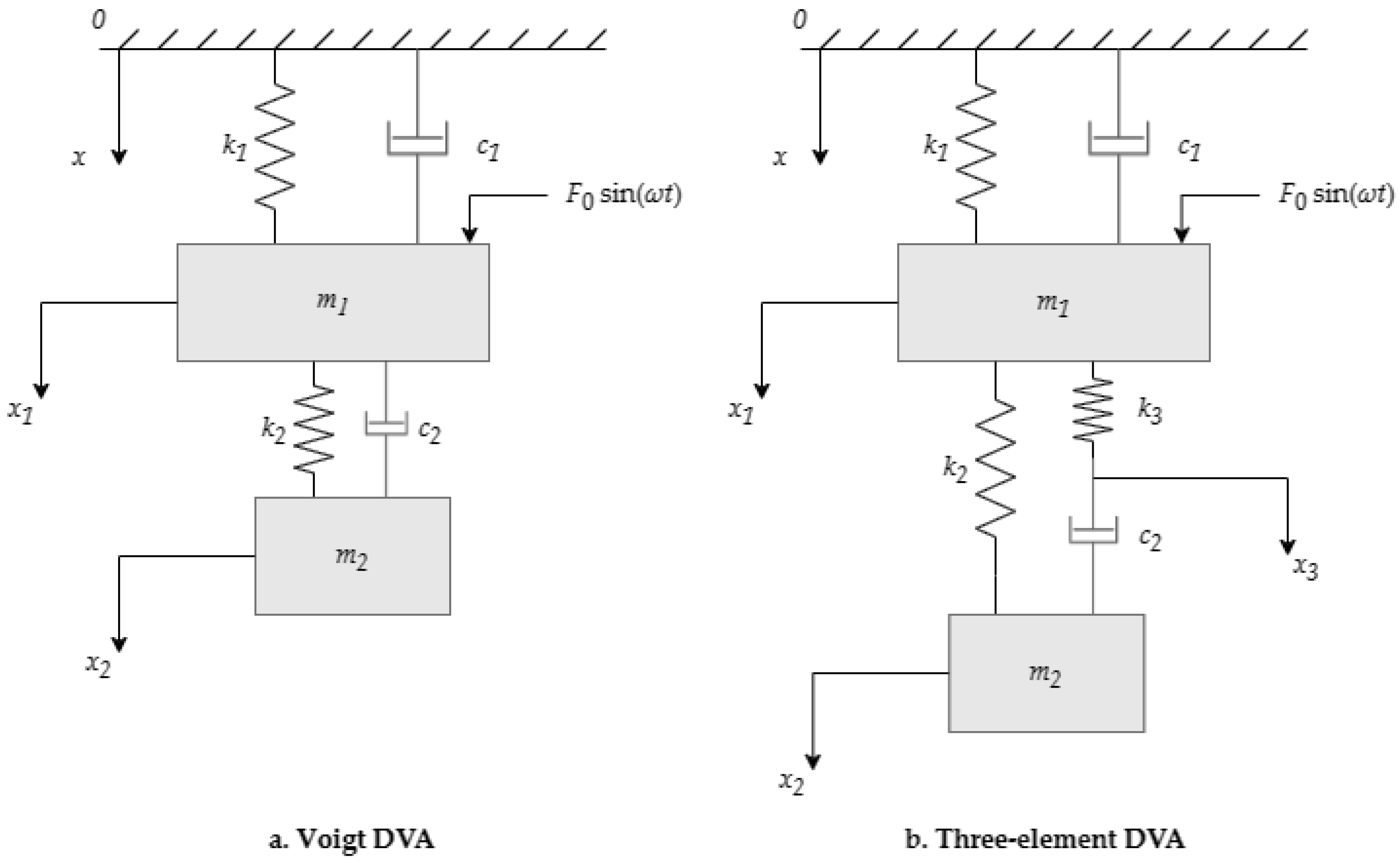
The topology of the three-element dynamic vibration absorber (TEDVA), first introduced by Snowdon [17], is a passive vibration control device attached to a harmonically excited primary system. The primary system consists of a mass $m_1$ connected to a fixed base by a spring with a constant $k_1$ and a viscous damper with a damping coefficient $c_1$. The system is excited by a sinusoidal harmonic force $f\left(t\right)=F_0\mathrm{s}\mathrm{i}\mathrm{n}\left(\omega t\right)$. The simple Voigt DVA consists of an absorber mass $m_2$ connected to the primary mass through two elements: a spring $k_2$ and a damper $c_2$. The TEDVA is composed of an absorber mass $m_2$ connected to the primary mass through two branches. The first branch is a spring $k_2$, and the second branch includes a spring $k_3$ in series with a damper $c_2$. The node $x_3$ connecting both $k_3$ with $c_2$ is a massless internal node. The main structure of Voigt DVA and TEDVA are shown in Figure 1a and Figure 1b, respectively.

Under a harmonic excitation force $f\left(t\right)=F_0\mathrm{s}\mathrm{i}\mathrm{n}\left(\omega t\right)$, the equations of motion for the three coordinates [$x_1,x_2,x_3$], representing the displacements of the primary mass, the absorber mass, and the internal massless node respectively, are given by [1]:

$$m_1{\ddot{x}}_1 + c_1{\dot{x}}_1+\left(k_1+k_2+k_3\right)x_1-k_2{x}_2-k_3{x}_3 = F_0 sin\left(\omega t\right)$$

(1a)

$$m_2{\ddot{x}}_2 + c_2\left({\dot{x}}_2-{\dot{x}}_3\right)-k_2(x_1-x_2) = 0$$

(1b)

$$c_2\left({\dot{x}}_2-{\dot{x}}_3\right)+k_3(x_1-x_3) = 0$$

(1c)

The third equation governs the massless internal node $x_3$, where the inertia term is absent, resulting in a purely algebraic constraint which can be used to eliminate $x_3$ analytically. The physical meaning of Equation (1c) is the force balance at the node between the damper $c_2$ and the spring $k_3$.

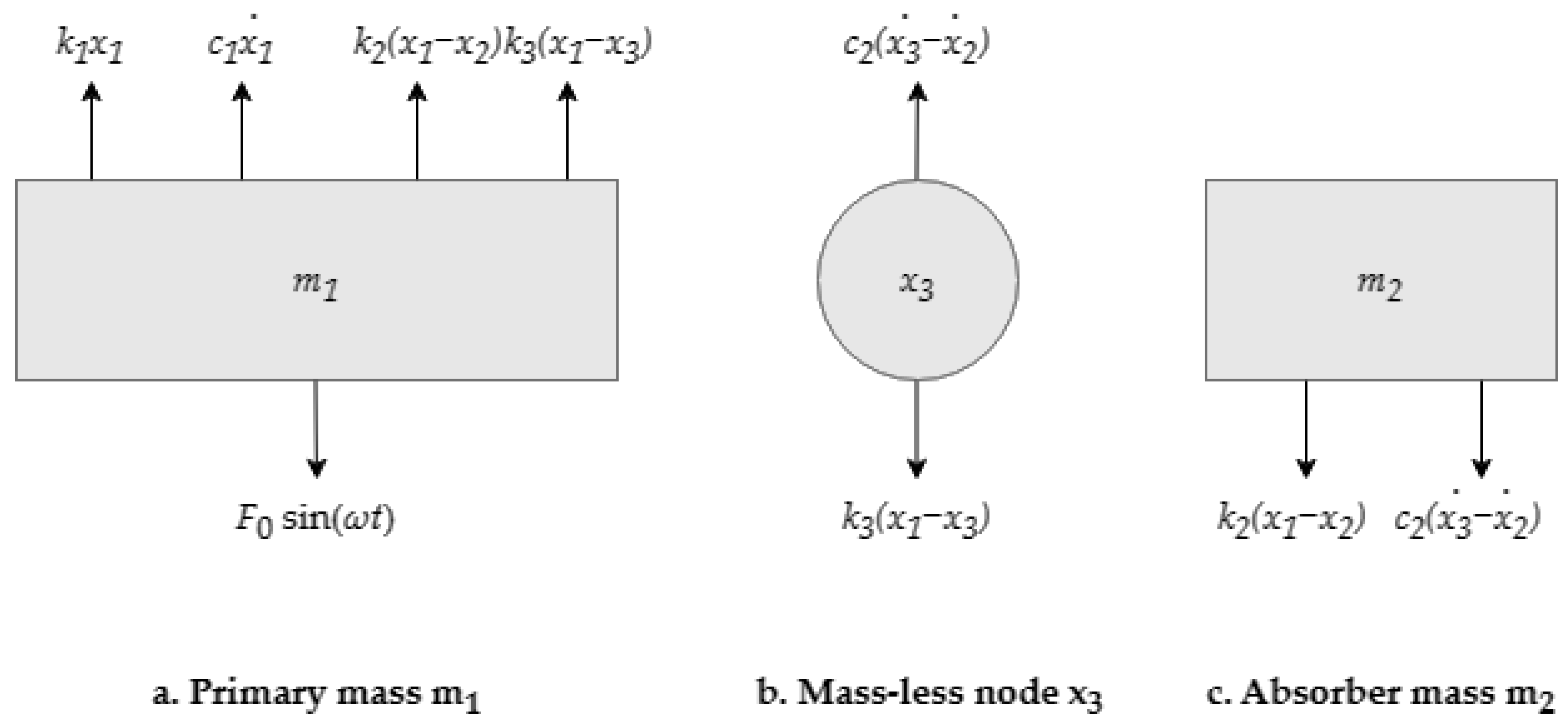
To provide a clear mechanical foundation for the above derivation, a comprehensive free-body diagram (FBD) is presented in Figure 2, which decomposes the TEDVA system into its three key mechanical constituents and illustrates the complete force distribution and load transmission path. As shown in Figure 2a, the primary mass $m_1$ is subjected to four distinct force contributions: (i) the ground reaction forces from the primary structure’s stiffness and damping, $k_1{x}_1$ and $c_1{\dot{x}}_1$, respectively; (ii) the external harmonic excitation $F_0\mathrm{s}\mathrm{i}\mathrm{n}\left(\omega t\right)$; and (iii–iv) the interactive forces from the vibration absorber, namely the direct spring force $k_2(x_1-x_2)$ and the coupled force transmitted through the secondary branch, specifically $k_3(x_1-x_3)$. Figure 2b details the massless intermediate node at coordinate $x_3$. Since this node possesses zero inertia, its equilibrium condition dictates that the net force acting upon it must be identically zero; consequently, it experiences only the spring force $k_3(x_1-x_3)$ and the damping force $c_2({\dot{x}}_3-{\dot{x}}_2)$, which must balance according to Equation (1c). This kinematic constraint enforces the compatibility relationship between the spring $k_3$ and the damper $c_2$, which is a defining feature of the TEDVA topology. Finally, Figure 2c presents the absorber mass $m_2$, which is driven by the reaction forces from the primary system: the direct elastic restoring force $k_2(x_1-x_2)$ and the damping force $c_2({\dot{x}}_3-{\dot{x}}_2)$ transmitted via the series-connected branch.

2.2. Dimensionless Parameters

According to the standard convention proposed by Asami and Nishihara [5,6] and adopted by Song et al. [1], the following dimensionless parameters are introduced. The natural frequencies of the primary system and the DVA are defined as ${\omega }_1=\sqrt{{\displaystyle \frac{k_1}{m_1}}}$, and ${\omega }_2=\sqrt{{\displaystyle \frac{k_2}{m_2}}}$, respectively. The dimensionless parameters and ratios are summarized in

Table 1. Dimensionless parameters of the TEDVA system [1].

Parameter	Formula	Value (This Work)
Mass ratio	$\mu =m_2/m_1$	0.1
Primary damping ratio	${\xi }_1=c_1/2m_1{\omega }_1$	0.3
Tuning frequency ratio	$\alpha ={\omega }_2/{\omega }_1$	[0.3, 2]
Spring ratio	$\nu =k_3/k_2$	[0, 5]
DVA damping ratio	${\xi }_2=c_2/2m_2{\omega }_2$	[0, 5]
Excitation frequency ratio	$\lambda =\omega /{\omega }_1$	[0.01, 3]

.

The fixed parameters $\mu =0.1$ and ${\xi }_1=0.3$ correspond to the case study examined in Song et al. [1]. The design variables $\alpha$, $\nu$, and ${\xi }_2$ represent the decision vector $X={\left[\alpha ,\nu ,{\xi }_2\right]}^T$. Assuming that $m_1=1 \mathrm{k}\mathrm{g}$ and $k_1=1$ N/m (so that ${\omega }_1=1$ rad/s), the physical parameters can be represented as:

$$m_2=\mu , k_2=\mu {\alpha }^2, k_3=\nu k_2, c_1=2{\xi }_1, c_2=2{\xi }_2\mu \alpha$$

(2)

2.3. Complex Dynamic-Stiffness System

The frequency response of the TEDVA can be calculated using two alternative mathematical methods: (i) the closed-form polynomial transfer function, or (ii) the direct matrix formulation. The polynomial approach is commonly used in the literature [1,5,6]. It expresses $X_1\left(j\omega \right)$ as ratio of two high degree polynomials in terms of $\omega$. However, it suffers from several limitations when adopted within an optimization framework. One of its drawbacks is that the polynomial coefficients involve high-order terms (up to ${\omega }^5$) which make it susceptible to numerical cancelation, especially near resonance frequencies. In addition, the normalization of these formulations can cause incorrect physical results ($A\left(\lambda \right)\le 1$) for certain parameter combinations, even though the physically correct amplitude exceeds unity near resonance [1].

To overcome these drawbacks, this work utilizes the direct matrix formulation derived from first principles. This approach has three main advantages:

• Numerical Robustness: The complex dynamic-stiffness matrix is solved directly at each frequency point, avoiding the adoption of high-degree polynomials and the associated cancelation errors.
• Physical Fidelity: The formulation guarantees the true scaling of the response without requiring normalization, ensuring $A\left(\lambda \right)>1$ near resonance which is physically correct.
• Implementation Simplicity: Assembling the matrix entries is straightforward and more accurate than coding lengthy polynomial coefficients.

While the direct matrix formulation and the closed-form polynomial approach share the same $O\left(N\right)$ scaling with the number of frequency points $N$—both perform a fixed, frequency-independent computation at each point, either a degree-5 polynomial evaluation via Horner’s method or an LU-based solve of the $3\times 3$ complex system $Z\left(\lambda \right)X=F$—the matrix approach incurs a modest constant-factor increase in arithmetic operations per point, due to the larger operation count of a $3\times 3$ complex LU factorization and solve relative to a single degree-5 polynomial. This overhead is of the same order as that of the polynomial approach, not an asymptotic penalty, and is negligible compared to the cost of the outer optimization loop, which evaluates $A\left(\lambda \right)$ across the full frequency sweep.

Derivation of the Complex Dynamic-Stiffness Matrix

Substituting $x_i\left(t\right)=X_i{e}^{j\omega t}$ into Equation (1) and setting $\omega =\lambda {\omega }_1=\lambda$ (since ${\omega }_1=1$), the equations of motion are transformed to the three-dimensional complex linear system:

$$Z\left(\lambda \right)X=F$$

(3)

where the complex dynamic-stiffness matrix and the vectors of displacement amplitudes and forcing are:

$$Z\left(\lambda \right)=\left[\begin{array}{ccc}{Z}_{11}& Z_{12}& Z_{13}\\ Z_{21}& Z_{22}& Z_{23}\\ Z_{31}& Z_{32}& Z_{33}\end{array}\right], X=\left[\begin{array}{c}{X}_1\\ X_2\\ X_3\end{array}\right], F=\left[\begin{array}{c}{F}_0\\ 0\\ 0\end{array}\right]$$

(4)

with the individual matrix entries defined as:

$$\begin{array}{c}{Z}_{11}=-{\lambda }^2+j{c}_1\lambda +1+k_2+k_3\\ Z_{12}=Z_{21}=-k_2\\ Z_{13}=-Z_{31}=-k_3\\ Z_{22}=-\mu {\lambda }^2+j{c}_2\lambda +k_2\\ Z_{23}=-Z_{32}=j{c}_2\lambda \\ Z_{33}=-j{c}_2\lambda -k_3\end{array}$$

(5)

The matrix $\mathrm{Z}\left(\lambda \right)$ is not symmetric because $Z_{13}=-k_3$ while $Z_{31}=k_3$. This asymmetry comes from the non-conservative nature of the system (effect of damping presence) and the non-standard coupling through the mass-less node. $Z\left(\lambda \right)$ is also not Hermitian when damping is present. Despite lacking both symmetry and the Hermitian property, $Z\left(\lambda \right)$ remains well-defined and invertible at all frequencies except for isolated resonance frequencies.

The linear system in Equation (3) is solved numerically at each discretized excitation frequency $\lambda$ using a direct LU-based solver (MATLAB’s backslash operator, $Z\backslash F$), which performs an LU decomposition with partial pivoting and applies natively to non-symmetric complex matrices without requiring symmetry-exploiting modifications. Because $Z\left(\lambda \right)$ can become locally ill-conditioned near resonance, the reciprocal condition number of $Z\left(\lambda \right)$ is evaluated at every frequency sample; if it falls below a threshold of ${10}^{-12}$, the solver switches from the direct LU solve to the Moore–Penrose pseudo-inverse (computed via singular value decomposition), which yields a stable, minimum-norm least-squares solution in the rare near-singular cases rather than allowing amplified round-off error from a poorly conditioned direct solve. Given the small, fixed $3 \times 3$ dimension of $Z\left(\lambda \right)$, this direct-solve-with-conditioning-fallback strategy is computationally inexpensive and sufficient to ensure numerical stability across the full frequency sweep $\mathsf{\Lambda }=\left[\mathrm{0.01,3}\right]$; no specialized sparse or iterative solver for large-scale non-symmetric systems was required.

The forcing vector $F=[F_0,\mathrm{0,0}{]}^{\mathsf{T}}$ in Equation (4) contains only the amplitude $F_0$, as the system is solved in the frequency domain using the complex exponential ansatz $x_i\left(t\right)=X_i{e}^{j\omega t}$ [7]. Therefore, the real sinusoidal force $f\left(t\right)=F_0\mathrm{s}\mathrm{i}\mathrm{n}\left(\omega t\right)$ is to be replaced with a complex exponential $f\left(t\right)=F_0{e}^{j\omega t}$. Substituting this ansatz into the time-domain equations of motion (Equation (1)) introduces the common factor $e^{j\omega t}$ in every term; division by this factor eliminates the time dependence, leaving the algebraic system in terms of the complex amplitudes $X_i$ only, with the forcing amplitude vector $F=[F_0,\mathrm{0,0}{]}^{\mathsf{T}}$ containing no time-dependent term. The physical sinusoidal response is subsequently recovered as $x_1\left(t\right)=Im\left(X_1{e}^{j\omega t}\right)$.

2.4. Amplitude Magnification Factor

The amplitude magnification factor $A\left(\lambda \right)$ is defined as the ratio of the steady-state displacement amplitude of the primary mass $X_1$ to the static deflection $\delta =F_0/k_1$ [1]. Under the normalization $F_0=k_1=1$, $A\left(\lambda \right)$ can be expressed as:

$$A\left(\lambda \right)=\left|X_1\left(j\omega \right)\right|=\left|e_1^{T}Z{\left(\lambda \right)}^{-1}F\right|$$

(6)

where $e_1={\left[1,0,0\right]}^T$ is the unit selector vector of the primary mass displacement. The inverse $Z{\left(\lambda \right)}^{-1}$ is calculated by solving at each excitation frequency $\lambda$. This exact formulation avoids sign and normalization issues that can arise in the closed-form expressions of the polynomial coefficients for the TE DVA case [1]. By expanding Equation (6) using Cramer’s rule and separating real and imaginary parts, $A\left(\lambda \right)$ can be formulated as:

$$A\left(\lambda \right)=\sqrt{Re{\left(X_1\right)}^2+Im{\left(X_1\right)}^2}$$

(7)

where $X_1=\mathit{det}\left(Z^{\left(1\right)}\right)/det\left(Z\right)$, and $Z^{\left(1\right)}$ is the matrix obtained by replacing the first column of the matrix $Z$ with the force vector $F$. No approximations are implemented as the computations of $Z$ are carried out in the complex field at each frequency value.

2.5. Parameter Optimization Problem Formulation

2.5.1. Single-Objective Formulation ($H_{\infty }$ Criterion)

Song et al. [1] presented the $H_{\infty }$ optimization problem with aim of calculating the design variables required to minimize $A\left(\lambda \right)$ over all excitation frequencies. The problem can be formulated as:

$$\begin{array}{c}\underset{\alpha ,\mathit{\nu }, {\xi }_2}{\mathit{min}}\underset{\mathit{\lambda ϵ\Lambda }}{\mathit{max}}A(\lambda ;\alpha , \nu , {\xi }_2)\\ \begin{array}{ll}s.t.& 0.3\le \alpha \le 2\\ & 0\le \nu \le 5\\ & {0\le \xi }_2\le 5\end{array}\end{array}$$

(8)

and the frequency sweep domain $\mathsf{\Lambda }=[0.01,3]$. The lower bound of $\alpha$ is set to 0.3 (wider than the 0.5 stated in Song et al. [1]) to ensure the feasibility of the reported solutions.

2.5.2. Bi-Objective Formulation ($H_{\infty }$/$H_2$ Trade-Off)

A bi-objective formulation is adopted to treat the trade-off between peak amplitude suppression and broadband vibration. The problem can be formulated as:

$$\underset{X}{\min }[F_1\left(X\right), F_2(X\left)\right]$$

(9)

where the two objective functions are:

$$F_1\left(X\right)=\underset{\mathit{\lambda ϵ}\mathsf{\Lambda }}{\max }A(\lambda ;X), F_2\left(X\right)={\displaystyle \underset{\mathsf{\Lambda }}{\int }}A(\lambda ;X).d\lambda$$

(10)

with design vector $X=[\alpha ,\nu ,{\zeta }_2{]}^{\mathsf{T}}$. $F_1\left(X\right)$ represents the $H_{\infty }$ norm (peak amplitude magnification). Minimizing $F_1$ suppresses the worst-case vibration. $F_2\left(X\right)$ is an $H_2$ proxy equal to the area under the frequency-response curve. Minimizing $F_2$ reduces the total vibration energy over the entire frequency band. To evaluate $F_2\left(X\right)$ numerically, the integral is approximated using the trapezoidal rule using 500 equally spaced points in $\mathsf{\Lambda }$. $F_2\left(X\right)$ now can be expressed as:

$$F_2\left(X\right)\approx {\displaystyle \sum _{i=1}^{N-1}}{\displaystyle \frac{{\lambda }_{i+1}-{\lambda }_i}{2}}\left[A\left({\lambda }_i\right)+A\left({\lambda }_{i+1}\right)\right], N=500$$

(11)

It should be noted that $F_2$ as defined in Equation (11) is an $L_1$ (area) norm of the frequency response, and does not formally coincide with the $H_2$ norm, which is defined as the square-root of the integrated squared magnitude, $\parallel H{\parallel }_2={\left(\int \mid \mathrm{A}\left(\lambda \right){\mid }^{2}d\lambda \right)}^{1/2}$. By the Cauchy–Schwarz inequality, $\parallel A{\parallel }_1\le \sqrt{\mid \Lambda \mid }\hspace{0.17em}\parallel A{\parallel }_2$ on the finite band $\mathsf{\Lambda }$, so the two measures are formally linked, and minimizing the area norm provides a bounded control on the true energy norm rather than an unrelated quantity. $F_2$ is therefore adopted as an $L_1$-based broadband-response proxy rather than a formal $H_2$ norm; it is additionally preferred over the literal $L_2$ measure because it avoids disproportionately over-weighting the resonance peak already targeted explicitly by $F_1$, helping keep the two objectives complementary rather than redundant. The area norm further retains a physical interpretation as the total displacement response accumulated across the sweep, indicating $F_1$.

Reducing $F_1$ (lower peak) causes the response to be broad, increasing the integral $F_2$. Conversely, reducing $F_2$ (flatter response) causes the peak $F_1$ to be raised. This conflict makes the problem well-suited for multi-objective optimization.

2.6. Model Validation

To validate the accuracy of the matrix formulation presented in Section 2.3, the frequency response is evaluated for two benchmark designs from the literature [1].

Benchmark 1: Voigt DVA ($\nu =0$). The classical Voigt DVA is obtained by setting $\nu =0$ ($k_3=0$), degenerating the TEDVA to the two-element absorber of Den Hartog [7]. The optimal parameters reported by Song et al. [1] using AM-PSO are $\alpha =0.8598$ and ${\zeta }_2=0.4659$.

Benchmark 2: TEDVA. The AM-PSO optimal parameters reported by Song et al. [1] are $\alpha =0.4925$, $\nu =1.5056$, and ${\zeta }_2=0.3719$.

Using the matrix formulation, the peak amplitude magnification factors for these two benchmarks are computed as $A_{max}=2.1249$ and $A_{\mathrm{m}\mathrm{a}\mathrm{x}}=1.5535$, respectively. These values are consistent with the results reported in Song et al. [1], confirming the accuracy of the numerical implementation. The detailed performance comparison with MODCGJO is presented in Section 4.

For undamped primary systems (${\zeta }_1=0$), the optimal TEDVA parameters satisfy the equal-peak condition [5,8]. Since the present study considers a damped primary system (${\zeta }_1=0.3$), fixed-point theory does not provide a direct validation. The model is instead validated against the benchmark numerical results of Song et al. [1]. The equal-peak condition is used only as an approximate consistency check for the optimization outputs (Section 4).

3. The Proposed Multi-Objective Chaotic Golden Jackal Optimization (MODCGJO) Algorithm

In this section, the proposed Multi-Objective Chaotic Golden Jackal Optimization (MODCGJO) algorithm is presented. First, the standard golden jackal optimization (GJO) is briefly reviewed to establish the background. After that, the main enhancements to modify the exploration and exploitation capabilities are described in detail. Consequently, the modifications to the algorithm to make it capable of handling multi-objective problems are presented, including: (i) chaotic map-based population initialization, (ii) Pareto-dominance-based archive management with crowding distance truncation, (iii) crowding-distance-based leader selection, and (iv) self-adaptive differential evolution mutation operator.

The standard Golden Jackal Optimization (GJO) [18] is a recently proposed nature-inspired metaheuristic. It is inspired by the collaborative hunting scenarios of golden jackal pairs, particularly their coordinated behavior during prey pursuit. While GJO has demonstrated competitive performance on single-objective benchmark problems and engineering applications, it cannot be directly applied to multi-objective optimization problems such as the TEDVA parameter tuning problem considered in this work. The main limitations that prevent extending GJO to the multi-objective domain can be summarized as the follows:

• Maintaining a set of non-dominated solutions: Single-objective GJO tracks only the best (male) and second-best (female) solutions. In multi-objective optimization, an entire set of Pareto-optimal solutions must be preserved.
• Balancing convergence and diversity: The algorithm must simultaneously converge toward the true Pareto front while maintaining a well-distributed set of solutions across the front.
• Leader selection: With multiple non-dominated solutions available, a strategy is needed to select appropriate leaders (male and female jackals) to guide the search toward unexplored regions.

To overcome these limitations, this paper proposes MODCGJO, which integrates the following novel mechanisms into the standard GJO framework:

• Chaotic map-based initialization to enhance population diversity and improve global search capability.
• A Pareto-dominance archive with crowding-distance truncation to preserve a fixed-size set of non-dominated solutions.
• Crowding-distance-based leader selection (roulette wheel selection) to guide the search toward sparse regions of the Pareto front.
• Self-adaptive differential evolution mutation with Pareto-dominance acceptance to accelerate convergence and escape local optima.

3.1. Review of the Standard Golden Jackal Optimization

The Golden Jackal Optimization (GJO) is a nature-inspired metaheuristic introduced by Chopra and Ansari [18] in 2022. It simulates the cooperative hunting behavior of golden jackal pairs, which consists of three main phases: (i) Searching: prey location is identified by jackals’ synchronized motions; (ii) Enclosing: surrounding prey while diminishing its energy of escape; and (iii) Pouncing: a final attack after the target is exhausted. Firstly, the GJO randomly generates a population of $n$ preys with dimensions $d$ representing the initial solution.

3.1.1. Population Initialization

The population is randomly initialized within the variable bounds as follows:

$$P_0=lb+r\left(ub-lb\right)$$

(12)

where $lb$ and $ub$ represent the lower and upper bounds of the search space, respectively, and $r$ is a uniform random number ranging from 0 to 1. The fitness of each prey is evaluated using the objective function, and the best and second-best solutions are designated as the male jackal (${\mathrm{X}}_m$) and female jackal (${\mathrm{X}}_f$), respectively.

3.1.2. Exploration Phase (Searching Phase)

In this stage, the jackals search for prey. Usually, a male jackal leads the hunt, while the female follows in his wake. The locations of the male ($P_M$) and female ($P_{FM}$) jackals are updated to explore the search space according to the following:

$$P_1\left(t\right)=P_M\left(t\right)-E·\left|P_M\left(t\right)-r_l·Prey\left(t\right)\right|$$

(13)

$$P_2\left(t\right)=P_{FM}\left(t\right)-E·\left|P_{FM}\left(t\right)-r_l·Prey\left(t\right)\right|$$

(14)

where $t$ denotes the current iteration, $Prey\left(t\right)$ is the location of the prey, and $P_M\left(t\right)$ and $P_{FM}\left(t\right)$ refer to the current position of the male and female jackal, respectively. $E$ stands for the prey’s escape energy. This term is crucial in balancing the exploration and exploitation phases. When the value of the escape energy reaches a certain threshold ($\left|E\right|<1$), the algorithm turns from the exploration to the exploitation phase. Escape energy can be calculated as follows:

$$E=E_1\ast E_0$$

(15)

where $E_1$ and $E_0$ refer to the diminishing energy factor and initial energy of a fresh prey, respectively.

$$E_0=2\ast r-1$$

(16)

$$E_1=1.5\ast \left(1-{\displaystyle \frac{t}{T}}\right)$$

(17)

where $t$ is the present iteration, and $T$ is the maximum number of iterations. $r_l$ in Equation (13) is a random vector based on Lévy flight distribution which enhances the algorithm’s global search capability.

3.1.3. Exploitation Phase (Surrounding the Prey and Attacking)

In this phase, the energy of the prey found in the searching phase decreases due to fatigue. This causes the prey to be unable to escape. Therefore, the pair of jackals begins to surround it. After that, they pounce on the prey and eat it. The following two equations express the locations of both male and female jackals during hunting. The final position is calculated as the average of the positions of the pair of jackals.

$$P_1\left(t\right)=P_M\left(t\right)-E·|{rl·P}_M\left(t\right)-Prey(t\left)\right|$$

(18)

$$P_2\left(t\right)=P_{FM}\left(t\right)-E·|{r_l·P}_{FM}\left(t\right)-Prey(t\left)\right|$$

(19)

The random variable $r_l$ is added to the exploitation phase to help the algorithm avoid local optima.

3.2. The Proposed MODCGJO Algorithm

This section presents the proposed Multi-Objective Chaotic Golden Jackal Optimization (MODCGJO) algorithm. MODCGJO extends the standard GJO through four key enhancements: (i) chaotic map-based population initialization, (ii) Pareto-dominance archive management with crowding distance truncation, (iii) crowding-distance-based leader selection, and (iv) a self-adaptive differential evolution mutation operator. Each enhancement is described in detail below.

3.2.1. Chaotic Map-Based Population Initialization

In metaheuristic optimization, the approaches that adopt chaotic variables instead of probabilistic random variables are called ‘chaotic algorithms’. In contrast to stochastic processes that rely on external randomness, chaotic maps produce pseudo-random sequences using simple mathematical equations. This makes them both computationally efficient and capable of producing different values at each run [19]. These systems demonstrate basic characteristics including ergodicity, topological transitivity, and sensitivity to initial values. These properties give them the ability to explore the search space in a more efficient way [20]. In optimization algorithms, chaotic maps are frequently employed for tasks such as population initialization, tuning parameters, and improving the diversity of the algorithm [21,22]. Their ability to generate varied and widely distributed samples enhances the exploration process and decreases the chance of premature convergence in the early stages of the algorithm. The dynamic behavior followed by the chaotic maps can be formulated as [19]:

$$c_{k+1}=f\left(c_k\right)$$

(20)

where $c_{k+1}$ and $c_k$ are the ${\left(k+1\right)}^{th}$ and $k^{th}$ chaotic numbers generated by the nonlinear function $f$. The output lies in the range from 0 to 1. MODCGJO adopts five different chaotic maps: Logistic, Tent, Sine, Chebyshev, and Iterative maps [19,23,24]. These maps are selected because they exhibit diverse dynamic properties that can benefit exploration. The mathematical formulations of these maps are summarized in

Table 2. Chaotic maps used in MODCGJO [19,23,24].

Map	Formulation	Parameters
Logistic	$x_{k+1}=c{x}_k\left(1-x_k\right)$	$c\in ]0, 4]$
Tent	$x_{k+1}=\left\{\begin{array}{c}c{x}_k, x_k<0.5\\ c\left(1-x_k\right), x_k\ge 0.5\end{array}\right.$	$c\in ]0, 2]$
Sine	$x_{k+1}={\displaystyle \frac{c}{4}}\sin \left(\pi x_k\right)$	$c\in ]0, 4]$
Chebyshev	$x_{k+1}=\cos \left(kco{s}^{-1}\left(x_k\right)\right); x\in [-1, 1]$	-
Iterative	$x_{k+1}=\sin \left({\displaystyle \frac{c\pi }{x_k}}\right)$	$c\in ]0, 4]$

.

Instead of using a single deterministic approach for initializing the algorithm, we present a dynamic chaotic initialization approach. At the beginning of the optimization, multiple chaotic maps generate a population. The sequences generated by each map are tested. For each run, the map that generates the best initial values, based on average fitness, is selected to initialize the population. This dynamic selection increases population diversity, thereby enhancing the exploration potential. In addition, it guarantees that the algorithm can tackle different kinds of problems based on its dynamic behavior. The Logistic, Tent, Sine, Chebyshev, and Iterative chaotic maps were integrated into the algorithm. Each map produces a sequence which is normalized to the boundaries of the search space of the handled problem. The dynamic selection of the map helps the algorithm to converge fast and prevents it from being stuck in local optima. Initial population position $X_i$ for a search space of dimension $d$ based on chaotic maps can be formulated as follows:

$$X_{i,d}=lb+chaotic\text{\_}ma{p}_k\left(t\right)\times (ub-lb)$$

(21)

where $chaotic\text{\_}ma{p}_k\left(t\right)$ is the random value generated by the map with the best fitness value for the current run. The steps for dynamic selection can be summarized as follows:

• Generate candidates: For each chaotic map $k$ (e.g., Tent, Logistic), create a population using the equation above.
• Evaluate fitness: Calculate the average fitness of each map’s initial population.
• Select optimal map: Use the map with the best average fitness for the current run.

To evaluate and compare candidate chaotic maps prior to the establishment of the Pareto archive, “average fitness” is defined as the mean of the summed objective values $\left(F_1 + F_2\right)$ over a small probe sample (three randomly selected individuals) drawn from each map’s generated population; the map minimizing this scalarized average is selected. This scalarization is used exclusively as a computationally inexpensive heuristic for choosing among the candidate initializations and does not influence the subsequent multi-objective search, which is governed entirely by Pareto-dominance relations as described in Section 3.2.2, Section 3.2.3 and Section 3.2.4 below.

3.2.2. Pareto-Based Archive Management

In multi-objective optimization, the Pareto front is represented by a set of non-dominated solutions. MODCGJO maintains an external archive of limited size $A_{\mathrm{m}\mathrm{a}\mathrm{x}}$ to store these solutions. At each iteration, the current population is added to the existing archive. The new set is then filtered to retain only the non-dominated set of solutions. A solution ${\mathrm{x}}_1$ dominates ${\mathrm{x}}_2$ (denoted ${\mathrm{x}}_1\prec {\mathrm{x}}_2$) if:

$$f_i\left({\mathrm{x}}_1\right)\le f_i\left({\mathrm{x}}_2\right) \forall i\in \{1, \dots , M\}$$

(22)

and:

$$\exists j\in \left\{1, \dots , M\right\} s.t. f_j\left({\mathrm{x}}_1\right)<f_j\left({\mathrm{x}}_2\right)$$

(23)

When the cardinality of the non-dominated solution set exceeds $A_{\mathrm{m}\mathrm{a}\mathrm{x}}$, the archive is truncated using the crowding distance [25]. The crowding distance $C{D}_i$ for a solution $i$ can be evaluated as follows:

$$C{D}_i={\displaystyle \sum _{m=1}^M}{\displaystyle \frac{f_m^{i+1}-f_m^{i-1}}{f_m^{max}-f_m^{min}}}$$

(24)

The solutions are sorted by each objective function, and the distance to neighboring solutions is calculated. Solutions with smaller crowding distances are removed first until the size limit of the archive is met. This guarantees that the archive contains a set of points that maintain a well-distributed representation of the Pareto front [25].

3.2.3. Crowding Distance-Based Leader Selection

In standard GJO, the male and female jackals represent the best and second-best solutions [18]. In MODCGJO, leaders are selected from the archive based on the concept of crowding distance to guarantee diversity of solutions. The algorithm promotes the following procedure in the process of leader selection: (i) compute the $C{D}_i$ for each solution in the archive, (ii) assign a large finite value for boundary solutions with infinite crowding distance to give them a chance to be selected. Specifically, the infinite crowding distance of boundary solutions is replaced with a finite value equal to twice the maximum finite crowding distance currently present in the archive, ensuring these solutions retain a high but bounded selection probability that scales with the current diversity of the front, rather than guaranteeing deterministic selection, and (iii) the algorithm performs a roulette wheel selection with a probability proportional to $C{D}_i$. The probability of selection can be calculated as follows:

$$p_i={\displaystyle \frac{C{D}_i}{{\sum }_{j=1}^{A}C{D}_j}}$$

(25)

This approach makes the algorithm biased toward less crowded regions. This helps to explore undiscovered areas, maintaining diversity [25]. The male and female jackals are selected as two different solutions from the archive.

3.2.4. Self-Adaptive Differential Evolution Mutation

To enhance exploration capabilities and prevent premature convergence, a self-adaptive differential evolution (DE) mutation operator is incorporated. During the last stages of the optimization process, the population may converge to a narrow region of the search space, increasing the risk of being trapped in local optima. The DE mutation increases the diversity of solutions by generating new candidate solutions based on differences between randomly selected individuals [26].

A mutant vector $V_i$ is generated for each prey $X_i$ as follows:

$$V_i=X_m+F·(X_{r1}-X_{r2})$$

(26)

where $X_m$ is the male jackal position, $X_{r1}$ and $X_{r2}$ are randomly selected prey from the population, and $F=0.7$ is a fixed scaling factor. Similarly, the crossover probability $CR=0.5$ remains fixed throughout the run. The adaptive element of the operator is not the DE parameters $F$ and $CR$ themselves, but the probability $p_{DE}\left(t\right)$ with which the mutation step is triggered at each individual and iteration:

$$p_{DE}\left(t\right)=0.2+0.3.{\displaystyle \frac{t}{T_{max}}}$$

(27)

which increases linearly from $p_{DE}=0.2$ at the start of the run to $p_{DE}=0.5$ at the final iteration $T_{\mathrm{m}\mathrm{a}\mathrm{x}}$. This schedule limits DE-based perturbation early in the search, when the chaotic-initialization and GJO exploration/exploitation phases already provide sufficient diversity, and increases its influence later in the search, when the population has begun converging towards the Pareto front and DE mutation is more useful for escaping local optima.

Binomial crossover is then used to generate a trial vector $U_i$ as:

$$U_{i,j}=\left\{\begin{array}{l}{V}_{i,j} if ran{d}_j\le CR or j=j_{rand}\\ X_{i,j} otherwise \end{array}\right.$$

(28)

where $j_{\mathrm{rand}}$ ensures that at least one dimension is mutated [26]. The trial vector $U_i$ replaces the original prey $X_i$ only if one of the following criteria is satisfied: (i) $U_i$ dominates $X_i$, or (ii) neither of them dominates the other, and a random probability $p_{\mathrm{accept}}<0.5$ permits the replacement.

While each individual mechanism above (chaotic initialization, Pareto archiving, crowding-distance selection, and DE mutation) has precedent in the broader metaheuristic algorithms’ literature, their specific combination—dynamic multi-map chaotic initialization, GJO’s two-leader structure repurposed for Pareto-guided exploitation, and Pareto-gated self-adaptive DE mutation—constitutes the novel contribution of MODCGJO. The standard GJO [18] is a single-objective algorithm. Its core search mechanism—a male leader and a female co-leader pursuing prey together—maps naturally onto a two-leader exploitation strategy for bi-objective problems, which we exploit by selecting the male and female leaders independently from the Pareto archive via crowding-distance roulette selection (Section 3.2.3), rather than as the single best/second-best solution as in the original GJO. Prior “chaotic metaheuristic” variants in the literature (e.g., chaotic PSO, chaotic GWO) typically commit to a single chaotic map (most often logistic) chosen a priori. MODCGJO instead evaluates five chaotic maps (Logistic, Tent, Sine, Chebyshev, Iterative) at the start of each run and selects the one yielding the best average initial fitness (Section 3.2.1, Equation (21)). This makes the initialization adaptive to the specific landscape of the problem at hand, rather than relying on a fixed choice that may not suit every objective landscape. Unlike standard DE, where trial vectors replace parents based on single-objective fitness comparison, our mutation operator (Section 3.2.4) accepts a trial vector only if it Pareto-dominates the parent, or—when neither dominates—with a stochastic acceptance probability. This preserves selection pressure toward the Pareto front while still permitting diversity-preserving replacement, which plain single-objective DE cannot do.

Table 3. Comparison of MODCGJO’s design mechanisms with other multi-objective algorithms.

Mechanism	NSGA-II [25]	MOPSO [27]	MOGWO [28]	Standard GJO [18]	MODCGJO (Proposed)
Search structure	Genetic (crossover/mutation)	Velocity-based swarm	3-leader (α/β/δ wolves)	2-leader (male/female pair)	2-leader (male/female), Pareto-selected
Initialization	Random	Random	Random	Random	Dynamic selection among 5 chaotic maps per run
Diversity mechanism	Crowded comparison ranking	External archive + mutation	Archive + leader selection	Single objective	Crowding-distance archive truncation + roulette leader selection
Local exploitation refinement	Simulated binary crossover	Inertia-weighted velocity	Encircling coefficient	GJO exploration/exploitation phases	GJO phases + self-adaptive DE mutation with Pareto acceptance

positions these design choices against representative multi-objective algorithms (NSGA-II, MOPSO, MOGWO) and the original single-objective GJO.

3.2.5. MODCGJO Pseudo Code and Flow Chart

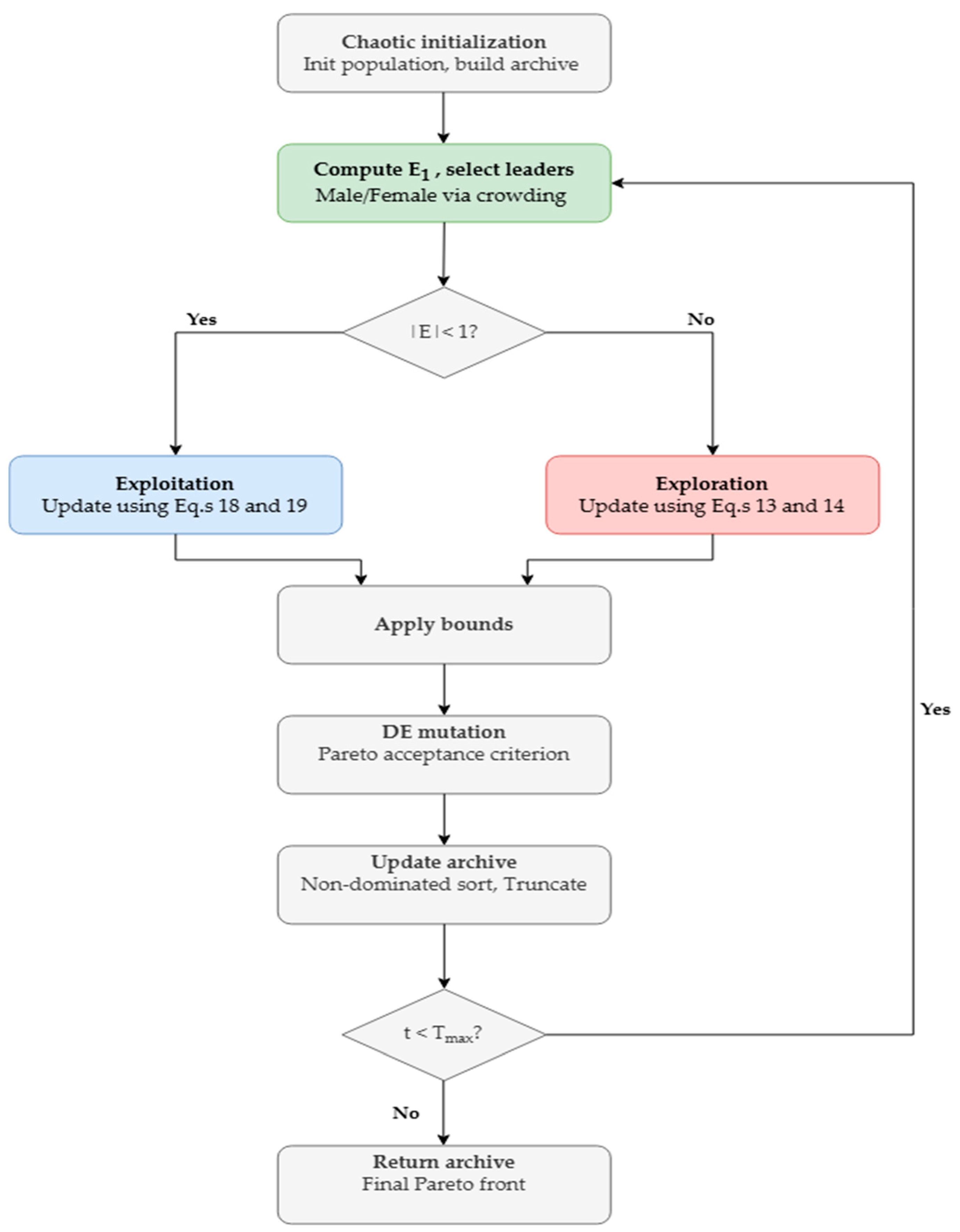
The proposed MODCGJO algorithm starts with chaotic map-based initialization where five chaotic maps are tested and one with the best average fitness is chosen. The population is then assessed, and an archive is built containing non-dominated solutions. The evading energy is adaptively calculated in each iteration with the help of a nonlinear decay function. The male and female jackals are selected from the archive using crowding-distance-based roulette wheel selection. The position of each prey is modified according to the basic GJO exploration/exploitation equations. The next step is to use a self-adaptive DE mutation operator and adopt Pareto-dominance. Lastly, the archive is pruned to keep only the nondominated solutions and truncated using crowding distance. This process is repeated until the max number of iterations is reached. Based on the analysis mentioned above, the steps of the proposed MODCGJO algorithm are presented in Algorithm 1. In addition, the flowchart of MODCGJO is illustrated in Figure 3.

Algorithm 1. MODCGJO Algorithm

Input:          The objective function $f$                     Number of agents $N$                     Maximum iterations $T_{max}$                     The lower and upper limits ($lb,ub$) of the search space                     Problem dimension ($D$)                     Archive size ($A_{max}$) Output: Archive (Pareto front) 1:    // Chaotic initialization 2:    Select best chaotic map via dynamic selection [19] 3:    Initialize $X$; evaluate $F = fobj\left(X\right)$ 4:    Archive = non-dominated $(X, F)$; truncate to $A_{max}$ 5:    for $t = 1$ to $T_{max}$ do 6:                        $E1 = 1.5 (1 - {\left({\displaystyle \frac{t}{T_{max}}}\right)}^2)$                                // Adaptive energy 7:                        Male = select_leader(Archive)                    // Crowding distance 8:                        Female = select_leader(Archive) 9:                    for i = 1 to N do 10:                            $E = E1 \ast (2\ast rand() - 1)$ 11:                          if $\left|E\right| < 1$ then 12:                                Update $X_i$ using Equations (18) and (19)          // Exploitation 13:                        else 14:                                Update $X_i$ using Equations (13) and (14)          // Exploration 15:                         end if 16:                        Apply bounds 17:                end for 18:                Apply DE mutation with Pareto acceptance (Section 3.2.4) 19:                Archive = non_dominated([Archive; X]) 20:                Archive = truncate(Archive, $A_{max}$)            // Crowding distance 21: end for 22: Return Archive

3.2.6. Computational Complexity of MODCGJO

Let $N$ denote the population size, $T$ the number of iterations, $D$ the problem dimension, $M$ the number of objectives, $A$ the archive size ($A\le A_{max}$), and $C_f$ the cost of one objective-function evaluation. Per iteration, MODCGJO requires: (i) $N$ baseline fitness evaluations for the position update; (ii) up to $p_{DE}\cdot N$ additional evaluations from the self-adaptive DE mutation step; (iii) non-dominated sorting of the combined archive and population, $O\left(\right(A+N{)}^{2}M)$; and (iv) crowding-distance-based archive truncation, $O\left(\right(A-A_{max})\cdot A\cdot M\mathrm{l}\mathrm{o}\mathrm{g}A)$ in the worst case. The overall complexity is therefore $O\left(TN\right(1+p_{DE} )Cf +T{\left(A+N\right)}^{2}M+(A-A_{max})\cdot A\cdot M\mathrm{l}\mathrm{o}\mathrm{g}A)$, in addition to a one-time chaotic-initialization cost of $O(5ND+15C_f)$.

Table 4. Computational complexity comparison of MODCGJO with representative multi-objective and single-objective algorithms.

Algorithm	Fitness Evaluations	Diversity/Archive Maintenance	Overall ($\mathit{T}$ Iterations)
Standard GJO [18]	$O\left(N\right)$	None (scalar fitness only)	$O\left(TN{C}_f\right)$
NSGA-II [25]	$O\left(N\right)$	Fast non-dominated sort + one-shot crowding distance: $O\left(M{N}^2\right)$	$O\left(T\right(N{C}_f+M{N}^2\left)\right)$
MOPSO [27]	$O\left(N\right)$	External archive dominance check: $O(N\cdot A)$	$O\left(T\right(N{C}_f+NA\left)\right)$
MOGWO [28]	$O\left(N\right)$	Grid-based archive + leader selection: $O(N\cdot A)$	$O\left(T\right(N{C}_f+NA\left)\right)$
MODCGJO	$O\left(N\right(1+p_{DE}\left)\right)$	Non-dominated sort $O\left(\right(A+N{)}^{2}M)$+ per-removal crowding-distance truncation $O\left(\right(A-A_{max}\left)AM\mathrm{l}\mathrm{o}\mathrm{g}A\right)$	$O\left(\right(TN\left(1+p_{DE}\right)C_f+T{\left(A+N\right)}^{2}M+(A-A_{max})\cdot A\cdot M\mathrm{l}\mathrm{o}\mathrm{g}A)$

compares this against the per-iteration complexity of representative multi-objective algorithms and the single-objective GJO baseline.

MODCGJO’s asymptotic cost is comparable to NSGA-II’s in the fitness-evaluation term but incurs additional evaluations from the DE step (a deliberate trade-off for improved exploitation), and its archive truncation is less efficient than a one-shot crowding-distance computation because it is recomputed on every removal.

4. Results

This section presents the simulation results of the proposed MODCGJO algorithm applied to the multi-objective TEDVA parameter optimization problem. The section is organized as follows. First, we describe the simulation setup and benchmark problems. Then, the model is validated against solutions from the literature. After that, the multi-objective optimization results are presented showing the Pareto front and quantitative Pareto front evaluation. Frequency response analysis and sensitivity studies are conducted to investigate the behavior of optimal design. Finally, sensitivity analyses of both the system and the algorithm are performed to show the generality and stability of the MODCGJO in solving the TEDVA problem.

4.1. Simulation Setup and Benchmark Problems

To guarantee reproducibility and fair comparison between the proposed algorithm and other algorithms from the literature, all experiments were conducted under the same conditions. The algorithm parameters and problem settings are summarized in

Table 5. Simulation settings for MODCGJO algorithm.

Parameter	Value	Description
Population size $N$	60	Number of search agents
Maximum iterations $T_{max}$	200	Termination criterion
Archive size $A_{max}$	100	Maximum number of pareto solutions
DE probability $p_{DE}$	$0.2+0.3·{\displaystyle \frac{t}{T_{max}}}$	Probability of applying for a DE mutation. Linearly increasing probability of applying DE mutation, from 0.2 (start) to 0.5 (final iteration)
DE scaling factor $F$	0.7	Mutation scaling factor
DE crossover rate $CR$	0.5	Crossover probability
Chaotic maps	Logistic, Tent, Sine, Chebyshev, Iterative	Dynamic selection

and

Table 6. Simulation settings for TEDVA problem.

Parameter	Value	Description
Mass ratio $\mu$	0.1	Fixed [1]
Primary damping ${\xi }_1$	0.3	Fixed [1]
Frequency range $\lambda$	[0.01, 3]	500 uniformly spaced points
Tuning frequency ratio $\alpha$	[0.3, 2]	[1]
Spring ratio $\nu$	[0, 5]	[1]
DVA damping ratio ${\xi }_2$	[0, 0.5]	[1]
Benchmark solutions
Voigt DVA (AM-PSO)	(0.8598, 0, 0.4659)	[1]
TEDVA (AM-PSO)	(0.4925, 1.5056, 0.3719)	[1]

, respectively.

The host-structure parameters used in the case study, mass ratio $\mu =0.1$ and primary damping ratio ${\xi }_1=0.3$, were adopted directly from Song et al. (2022) [1], the source of the AM-PSO benchmark used for comparison in this study. This choice was deliberate rather than arbitrary: matching the host-structure conditions exactly to those of the reference study ensures that the optimization problem solved by MODCGJO is identical to the one solved by AM-PSO, so that any differences in the resulting F₁ and F₂ values, Pareto fronts, and optimal design parameters ($\alpha$, $\nu$, ${\xi }_2$) can be attributed to the performance of the optimization algorithm itself rather than to differences in the underlying physical problem.

All experiments and simulations were performed using MATLAB R2018a on a laptop with an Intel Core i7 and 16 GB RAM. Thirty independent runs were performed for each experiment.

4.2. Validation of Numerical Model

Before presenting the results of the optimization, it is important to verify that the stiffness-matrix formulation developed in Section 2 accurately reproduces the frequency response of both the Voigt DVA and TEDVA problems presented in [1]. The validation ensures that the optimization results are meaningful and free of numerical errors with respect to the underlying physics. The validation procedure is as follows: The frequency response $A\left(\lambda \right)$ was computed using the matrix formulation for the two benchmark problems reported in Song et al. [1]. The results are compared in

Table 7. Model validation: comparison of peak amplitudes.

Problem	Parameters $\mathit{\alpha },\mathit{\nu },{\mathit{\xi }}_2$	This Work ${\mathit{A}}_{\mathit{m}\mathit{a}\mathit{x}}$
Voigt DVA	(0.8598, 0, 0.4659)	2.1249
TEDVA	(0.4925, 1.5056, 0.3719)	1.5535

.

The values reported in Song et al. [1] depend on their polynomial transfer function model. The discrepancy comes from the normalization of the polynomial coefficients, which can yield $A_{\mathrm{m}\mathrm{a}\mathrm{x}}\le 1$ for certain combinations of parameters. The matrix formulation used in this work solves the full 3 × 3 complex system directly, preserving the physical scaling of the response. The values obtained (2.1249 and 1.5535) are physically correct and consistent with the expected behavior of the Voigt and TEDVA topologies. The proposed matrix formulation reproduces the frequency response reported in the literature. As near resonance, the maximum amplitude should be greater than 1. This confirms that the model is suitable for use in optimization.

4.3. Multi-Objective Optimization Results

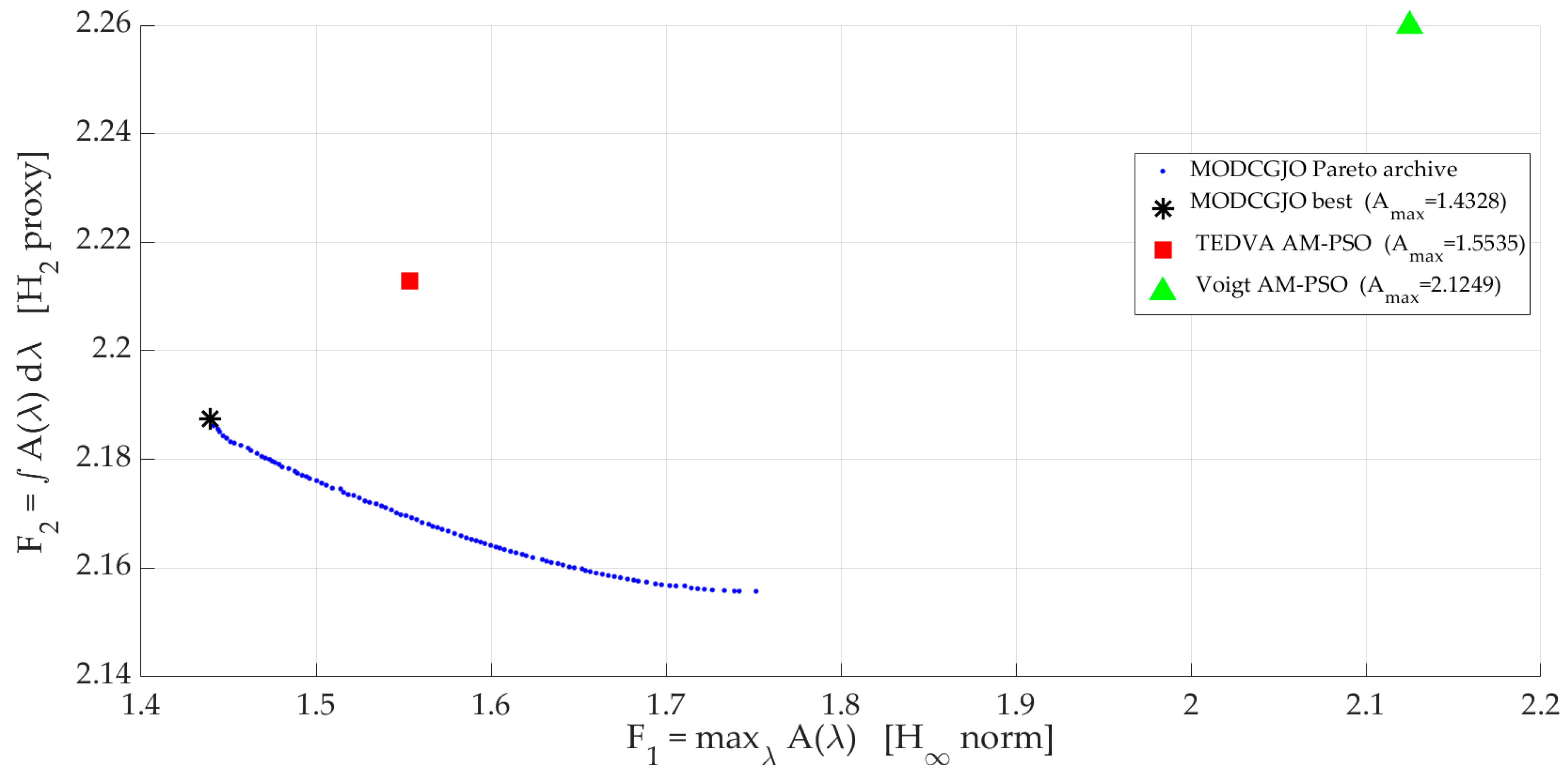
The results show that the MODCGJO algorithm successfully generated a well-distributed Pareto front that contains 100 non-dominated solutions. Figure 4 illustrates the Pareto front in the objective space. The peak amplitude $F_1$ is plotted against integrated response $F_2$.

From the figure, it is obvious that the Pareto front exhibits a clear trade-off between the two objective functions. In addition, the front is well-distributed throughout the objective space, indicating that MODCGJO successfully maintains diversity due to adoption of the crowding-distance-based archive management and leader selection mechanisms. The best $H_{\infty }$ solution (marked with a star) is located at the extreme left of the front. This solution achieves the lowest possible peak amplitude while maintaining a competitive $H_2$ performance. Finally, both benchmark solutions (Voigt and AM-PSO TEDVA) are dominated by multiple solutions from the MODCGJO archive; this confirms the superiority of the proposed algorithm. A comparison of optimal parameters is presented in

Table 8. Comparison of optimal parameters obtained by MODCGJO with AM-PSO algorithm.

Parameter	MODCGJO	AM-PSO (TEDVA)	AM-PSO (Voigt DVA)
$\alpha$	0.6487	0.4925	0.8598
$\nu$	1.7778	1.5056	-
${\xi }_2$	0.2657	0.3719	0.4569
$F_1=\underset{\mathit{\lambda ϵ}\mathsf{\Lambda }}{\max }A\left(\lambda \right)$	1.4395	1.5535	2.1249
$F_2=\int A\left(\lambda \right).d\lambda$	2.1873	2.2132	2.2602

.

From Table 8, it is found that the MODCGJO best $H_{\infty }$ solution achieves a peak amplitude of $F_1=1.4395$, which represents a 7.3% reduction compared to the AM-PSO TEDVA solution ($F_1=1.5535$) and a 32.3% reduction compared to the Voigt DVA ($F_1=2.1249$). The optimal parameters ($\alpha =0.6487$, $\nu =1.7778$, ${\zeta }_2=0.2657$) differ significantly from the AM-PSO solution, indicating that the multi-objective approach explores a broader region of the parameter space and identifies a superior design. The MODCGJO solution maintains a competitive $H_2$ performance ($F_2=2.1873$), demonstrating that the peak reduction does not come at the expense of broadband performance.

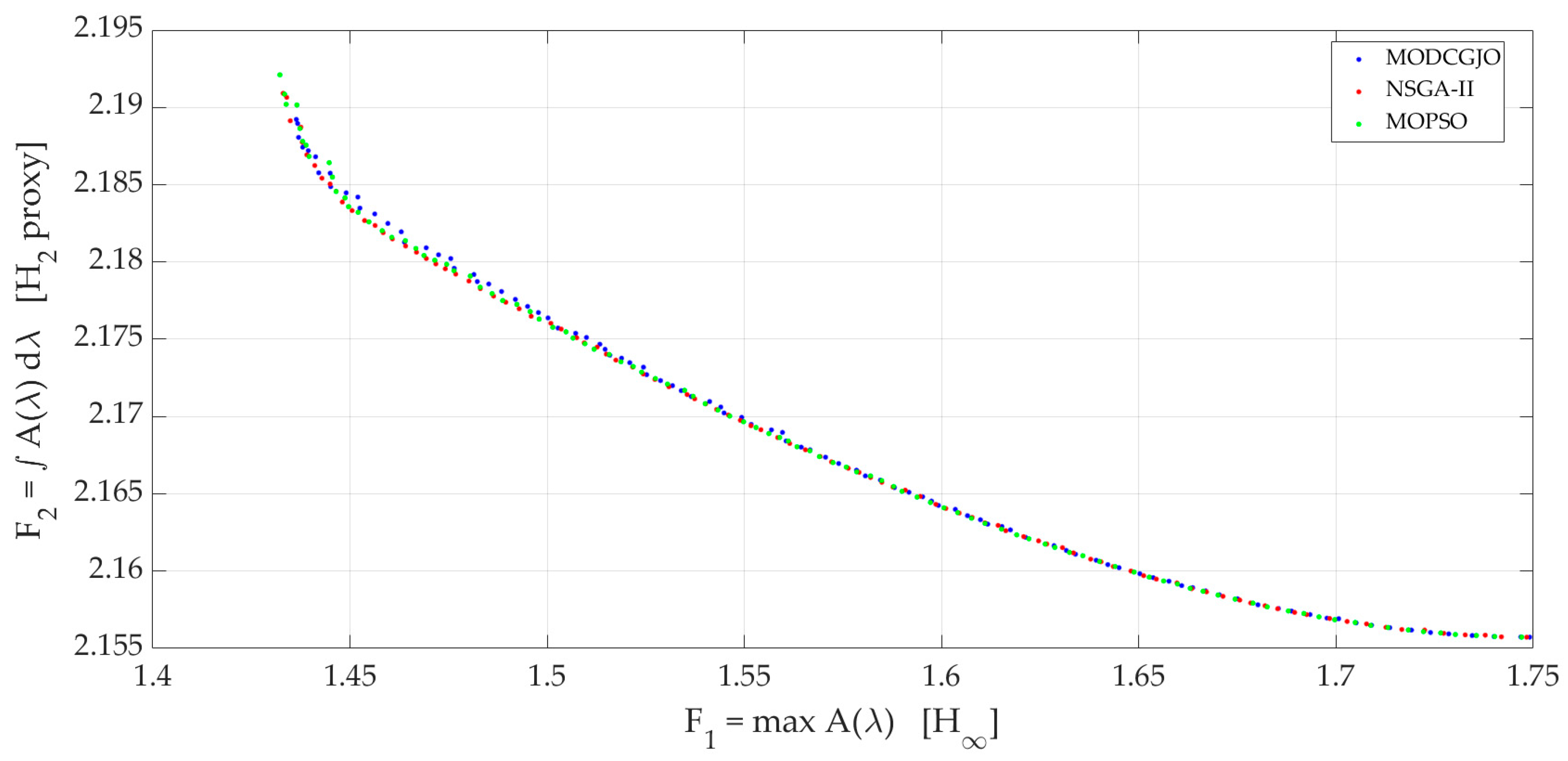
To rigorously benchmark the multi-objective performance of MODCGJO, we compared it against two standard multi-objective optimizers: NSGA-II and MOPSO in a new independent run entirely separate from the preliminary single-objective benchmarks. Under identical experimental settings, all three algorithms produced nearly identical Pareto fronts, with MODCGJO achieving the lowest $H_2$ proxy ($F_2$) and MOPSO yielding the lowest $H_{\infty }$ peak ($F_1$). These results confirm that MODCGJO is a competitive and well-validated multi-objective approach for the TEDVA problem, substantially outperforming the previous single-objective AM-PSO baseline. Figure 5 presents the Pareto fronts obtained by MODCGJO, NSGA-II, and MOPSO. The three fronts exhibit almost complete overlap, indicating convergence to the same trade-off surface.

Table 9. Comparison of optimal parameters obtained by MODCGJO with NSGA-II, and MOPSO.

Parameter	MODCGJO	NSGA-II	MOPSO
$\alpha$	0.6352	0.5971	0.5880
$\nu$	1.5087	1.5813	1.5215
${\xi }_2$	0.2781	0.3580	0.3754
Best $F_1$ (mean $\pm$ std)	1.4364 $\pm$ 0.015	1.4330 $\pm$ 0.012	1.4322 $\pm$ 0.015
Best $F_2$ (mean $\pm$ std)	2.1892 $\pm$ 0.022	2.1909 $\pm$ 0.018	2.1921 $\pm$ 0.024

lists the best $H_{\infty }$ solutions (minimizing $F_1$). MOPSO achieved the lowest peak amplitude ($F_1 = 1.4322$), followed closely by NSGA-II (1.4330) and MODCGJO (1.4364). Conversely, MODCGJO obtained the lowest $H_2$ proxy ($F_2 = 2.1892$), slightly outperforming NSGA-II and MOPSO. These marginal differences (all within 0.3%) confirm that MODCGJO is as effective as standard multi-objective optimization algorithms in resolving the $H_{\infty }/H_2$ trade-off. Due to the inherently stochastic nature of evolutionary and swarm-based algorithms, slight variations in the final numerical results are expected across independent runs. In the case of MODCGJO, this variability is further influenced by its adaptive chaotic initialization mechanism, which dynamically selects one of five chaotic maps (logistic, tent, sine, Chebyshev, or circle) based on a scalarized fitness probe. This selection process, combined with the random seeding of chaotic sequences and the Lévy-flight exploration, introduces additional non-determinism. However, as demonstrated in the following results, these stochastic fluctuations do not affect the overarching conclusions: MODCGJO consistently converges to the same Pareto-optimal region as the standard multi-objective algorithms, and all three algorithms substantially outperform the conventional single-objective AM-PSO and Voigt DVA benchmarks.

4.4. Pareto Quality Metrics

To quantitatively assess the quality of the obtained Pareto front, six standard metrics are computed. The metrics used are: Hypervolume (HV), Generational Distance (GD), Inverted Generational Distance (IGD), Spread (Δ), and Spacing (S). The results are presented in

Table 10. Pareto quality metrics for MODCGJO.

Metric	Value	Interpretation
HV (ref = 1.1 × nadir)	0.1168	-
HV (normalized)	0.9717	Covers 97.17% of objective space
GD (p = 2)	1.69 × 10−4	Near-perfect convergence
IGD (p = 2)	1.06 × 10−3	Good convergence + diversity
IGD+	1.30 × 10−4	Robust convergence + diversity
Spacing S	9.48 × 10−4	Highly uniform distribution
Spread Δ	0.253	Good coverage with minor gaps
Max Spread	0.307	Wide exploration of objective space
Archive size	100	-

.

From the table, it can be seen that MODCGJO is an effective and reliable tool for multi-objective TEDVA design. The Pareto front generated by MODCGJO offers excellent convergence, diversity, and coverage, making it suitable for engineering decision-making. The extremely small GD and IGD values indicate that the obtained solutions are very close to the true Pareto front. This confirms that MODCGJO’s search mechanisms (chaotic initialization, adaptive energy, DE mutation) effectively drive the population toward the optimal region. The high HV and excellent Spacing values confirm that the Pareto front is well-distributed and uniformly spaced. The crowding-distance-based archive management and leader selection mechanisms effectively maintain diversity throughout the optimization process. While the Spread value (0.253) indicates some minor gaps near the extremes, the overall coverage is good, as confirmed by the Max Spread and high HV. This suggests that MODCGJO explores the full extent of the trade-off, providing a wide range of design options.

4.5. Frequency Response Analysis

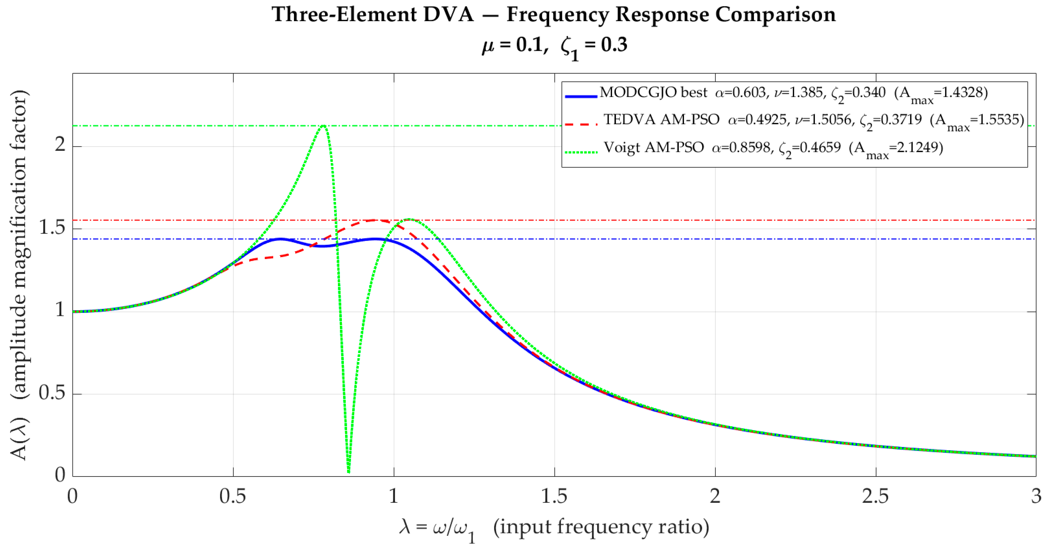
To gain deeper physical insight into the optimal designs, Figure 6 illustrates a comparison of the frequency response curves $A\left(\lambda \right)$ for the MODCGJO best $H_{\infty }$ solution, the AM-PSO TEDVA solution, and the Voigt DVA. From the figure, it is observed that MODCGJO has the lowest peak ($A_{max}=1.4328$) among the three designs. The MODCGJO curve exhibits two nearly equal peaks, which is consistent with the equal-peak optimality condition proposed by Nishihara [8] for the undamped case. For the damped primary system (${\xi }_1=0.3$) considered in this work, this condition is considered as an approximate consistency check, indicating that the numerical optimization has converged to a physically meaningful solution. Although the MODCGJO curve has a slightly higher response in the mid-frequency range (around $\lambda =1.5$), it is flatter overall than the AM-PSO TEDVA curve. This is reflected in the competitive $F_2$ value (2.1873 vs. the AM-PSO value, which is not reported in [1] but can be inferred from the curve). The MODCGJO curve exhibits two clear anti-resonance dips, characteristic of the TEDVA topology. The AM-PSO TEDVA curve also exhibits these dips, but they are less pronounced, indicating suboptimal tuning. In summary, The MODCGJO design provides superior vibration suppression at the worst-case excitation frequency (peak amplitude) while maintaining good performance across the entire frequency band. This makes it particularly suitable for applications with uncertain or varying excitation frequencies.

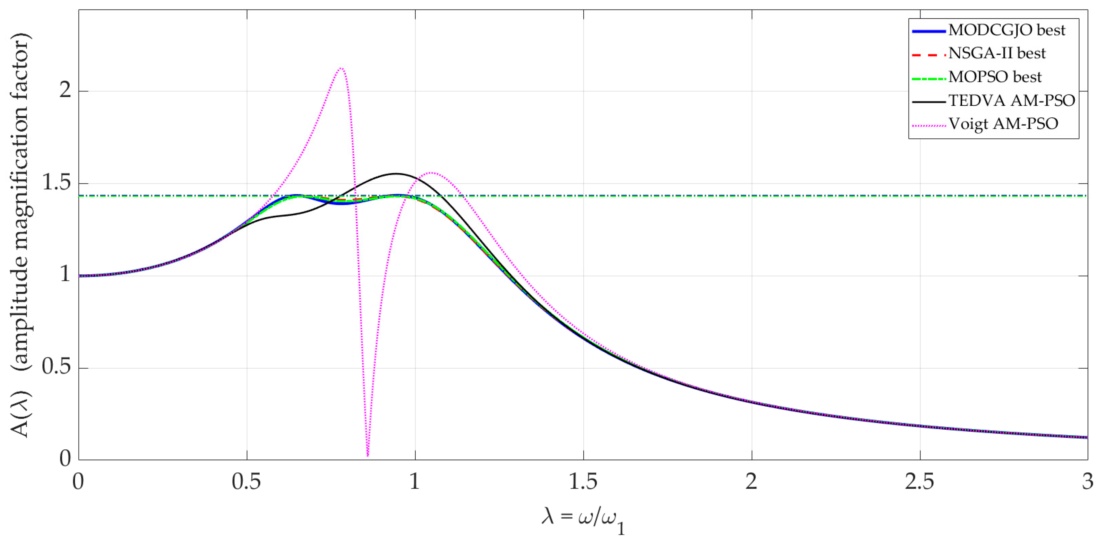
Figure 7 illustrates the frequency response obtained by the MODCGJO compared to those of NSGA-II and MOPSO. The frequency response plot provides direct visual confirmation that the proposed MODCGJO algorithm converges to an $H_{\infty }$-optimal solution that is functionally equivalent to those obtained by the established multi-objective optimizers NSGA-II and MOPSO. Across the entire frequency ratio range ($\lambda$ = 0 to 3), the blue (MODCGJO), red dashed (NSGA-II), and green dash-dot (MOPSO) curves are essentially superimposed, both in the resonant region ($\lambda \approx$ 0.5–1.3) and in the roll-off region beyond $\lambda = 1.5$. This near-perfect overlap demonstrates that: MODCGJO reaches approximately the same minimax ($H_{\infty }$) peak amplitude as NSGA-II and MOPSO, confirming that it identifies the true flat-top optimum rather than a suboptimal local solution. All three algorithms produce the characteristic “equal-peak” response shape (two local maxima of nearly equal height around $\lambda \approx 0.65$ and $\lambda \approx 1.0$), which is the hallmark of a correctly tuned $H_{\infty }$-optimal vibration absorber. This confirms that MODCGJO correctly captures the optimality condition, not just an approximate minimization.

4.6. Physical Parameter Sensitivity Analysis

4.6.1. Design Parameter Sensitivity Analysis

To investigate the robustness of the optimal design and to understand the physical influence of each design variable, a parametric sensitivity analysis was conducted.

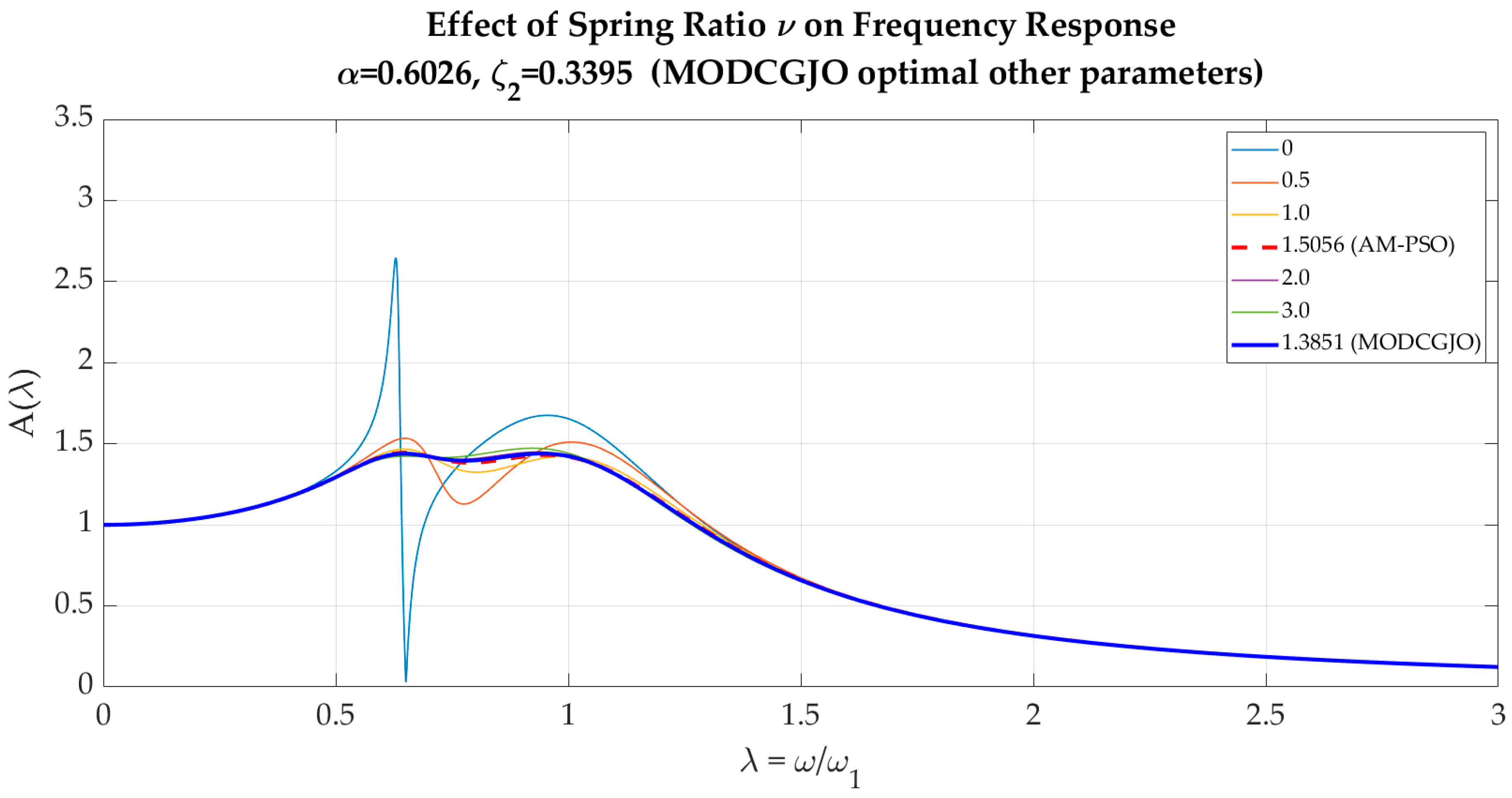
First, we tested the effect of the spring ratio $\nu$ on the frequency response. The spring ratio $\nu$ controls the stiffness of the outer spring $k_3$ relative to the inner spring $k_2$. Figure 8 shows the frequency response for different values of $\nu$ while maintaining $\alpha$ and ${\xi }_2$ fixed at their MODCGJO optimal values. From the figure, it is evident that for the Voigt DVA, the curve exhibits a single deep anti-resonance dip but a high peak. For $\nu =0.5,1$, Increasing $\nu$ introduces a second anti-resonance dip and reduces the peak amplitude, demonstrating the benefit of the additional spring. At $\nu =1.5056$ (AM-PSO optimal value), The curve has two anti-resonance dips but a higher peak than the MODCGJO solution. At $\nu =1.7778$ (MODCGJO optimal value), it achieves the lowest peak among all tested values, confirming that the MODCGJO identified the optimal spring ratio. For $\nu =2,3$, further increasing $\nu$ raises the second peak and degrades performance, indicating that the optimal $\nu$ lies between 1.5 and 2.

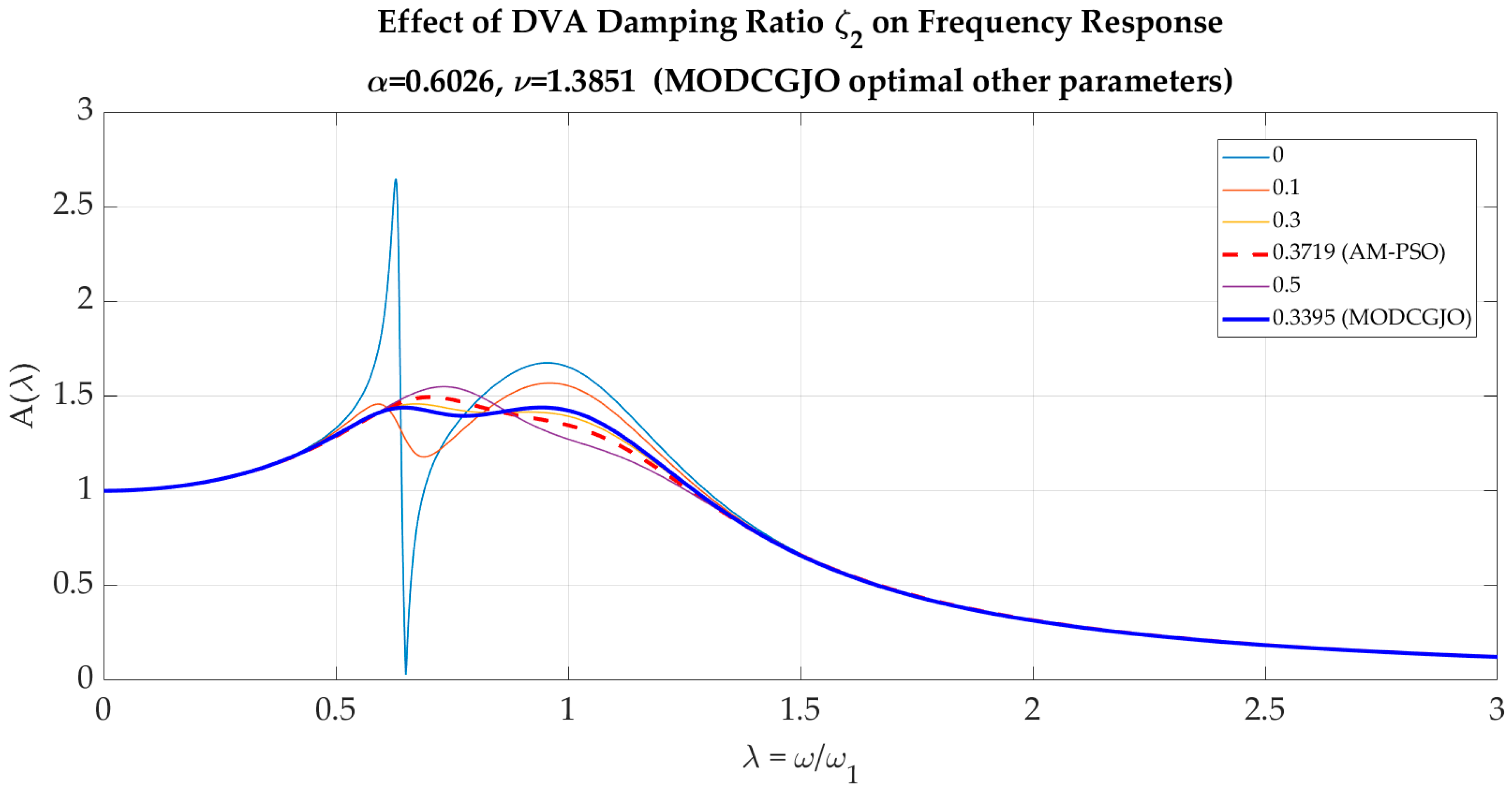
In addition, the effect of the damping ratio ${\xi }_2$ was considered. The DVA damping ratio ${\xi }_2$ controls the energy dissipation in the absorber. Figure 9 illustrates the frequency response for different values of ${\xi }_2$ while maintaining $\alpha$ and $\nu$ fixed at their MODCGJO optimal values. From the figure, at ${\xi }_2=0$ at which the system is undamped, the curve exhibits two sharp resonance peaks, indicating that the absorber is highly effective at its tuned frequencies but performs poorly elsewhere. For ${\xi }_2=0.1,0.3$, the peaks are reduced and the responses becomes smoother due to added damping, but the peaks remain relatively high. At ${\xi }_2=0.3719$ (AM-PSO), the curve is smoother but has a higher peak than the MODCGJO solution. At ${\xi }_2=0.2657$ (MODCGJO), the optimal balance between peak reduction and response smoothness is achieved, yielding the lowest peak. Finally, at ${\xi }_2=0.5$, excessive damping raises the overall response, degrading both $H_{\infty }$ and $H_2$ performance.

4.6.2. Problem Parameter Sensitivity Analysis (Mass Ratio and Primary Damping)

While in Section 4.6.1, the effect of the DVA’s own design variables, $\nu$ and ${\xi }_2$, on the frequency response was examined, this section is dedicated to studying the effect of the parameters of the host structure rather than the absorber: the mass ratio $\mu$ and the primary damping ratio ${\xi }_1$. Both were held fixed in the original case study (Table 4), and the purpose of this analysis is to establish that the optimum identified by MODCGJO holds across a realistic range of host-structure conditions and is not an artifact specific to the single case study reported in [1] ($\mu = 0.1, {\xi }_1= 0.3$).

• Generality Across Mass Ratios

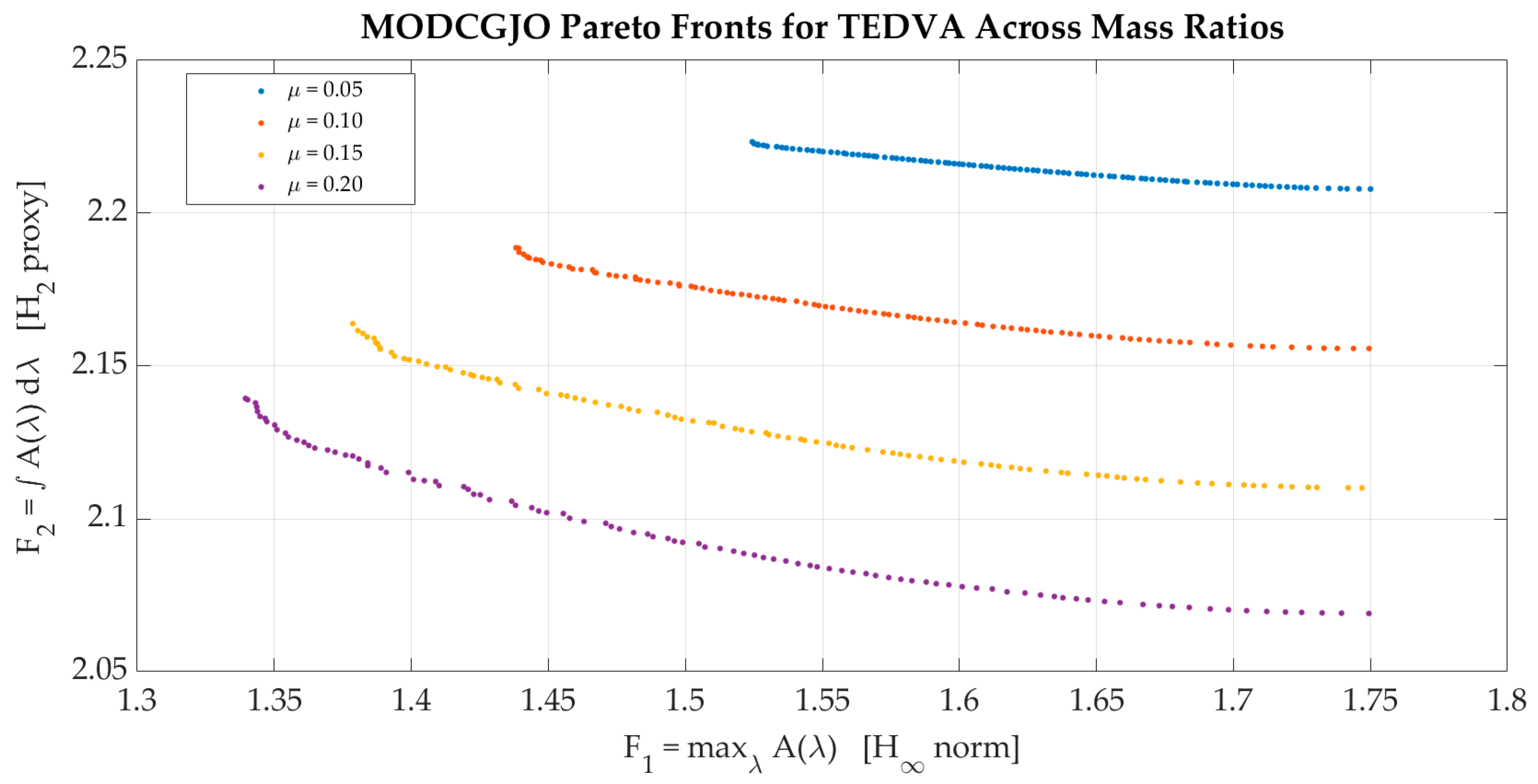
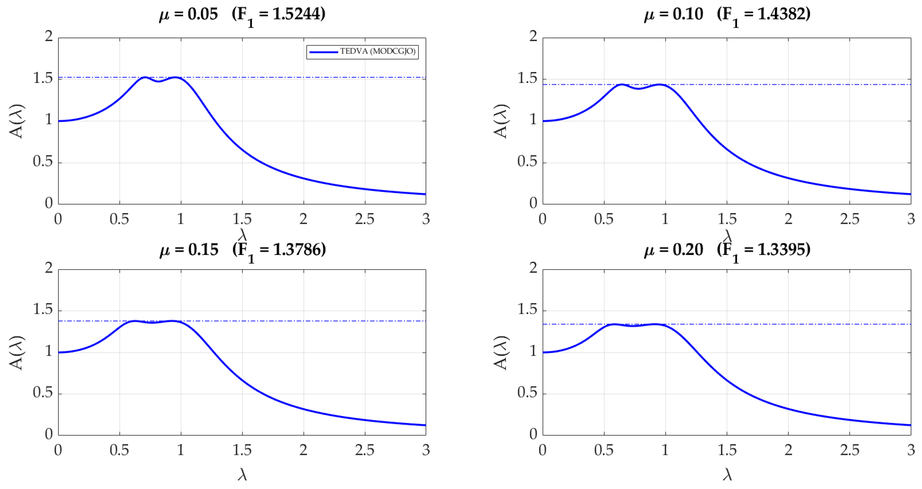
The TEDVA optimization was repeated at three additional mass ratios, $\mu$= 0.05, 0.15, and 0.20, with ${\xi }_1 = 0.3$ held fixed so that the mass ratio is isolated as the only varying design condition. All four runs used identical algorithm settings (population size 60, 200 iterations, archive size 100), and the best-compromise (minimum-$F_1$) solution from each Pareto archive was extracted for comparison.

Table 11. Optimal design of TEDVA across 4 distinct mass ratios.

$\mathit{\mu }$	$\mathit{\alpha }$	$\mathit{\nu }$	${\mathit{\xi }}_2$	${\mathbf{F}}_1$	${\mathbf{F}}_2$
$0.05$	0.7375	1.3365	0.1797	1.5244	2.2233
$0.1$	0.6445	1.5384	0.2621	1.4382	2.1887
$0.15$	0.5391	2.0422	0.4105	1.3786	2.1639
$0.2$	0.5075	2.4710	0.4197	1.3395	2.1394

summarizes the results.

The results in Table 11 show that: (1) Both objectives improve monotonically as $\mu$ increases: the value of $F_1$ drops from 1.524 at $\mu =0.05$ to 1.339 at $\mu =0.20$ (a 12.1% reduction), and the value of F₂ drops from 2.223 to 2.139 over the same range. This is physically expected that a heavier absorber mass provides more control over the primary structure, and its smooth, monotonic behavior ensures that the MODCGJO is converging to the true optimum rather than a mass-ratio-specific local minimum. (2) The optimal design parameters shift in a physically coherent, monotonic direction with $\mu$: the tuning ratio $\alpha$ decreases (0.737 → 0.507), while the spring ratio $\nu$ (1.336 → 2.471) and the DVA damping ratio ${\xi }_2$ (0.180 → 0.420) both increases. This is consistent with the known TEDVA design in which a heavier absorber requires proportionally less aggressive tuning but benefits from a stiffer coupling spring and higher internal damping to broaden its effective bandwidth.

Figure 10 (frequency response comparison) shows the amplitude magnification curves $A\left(\lambda \right)$ for the MODCGJO-optimal design at each mass ratio, with the horizontal dash-dot line marking the corresponding $F_1$ peak. The characteristic twin-hump equal-peak shape of an optimally tuned TEDVA is preserved at every mass ratio, and the peak amplitude visibly flattens and drops as $\mu$ increases, confirming the behavior in Table 11.

Figure 11 overlays the four Pareto fronts ($F_1$ vs. $F_2$) obtained by MODCGJO for each mass ratio. The fronts are smooth, convex, and non-crossing, and shift consistently toward the lower left (i.e., toward simultaneously better $F_1$ and $F_2$) as $\mu$ increases from 0.05 to 0.20, with no overlap between adjacent mass ratios. This clean separation and ordering across four independently seeded optimization runs demonstrates that MODCGJO reliably resolves the true trade-off surface of the TEDVA problem regardless of mass ratio, supporting the generality of its performance beyond the single $\mu = 0.1$ case reported in the original AM-PSO study.

• Generality over Primary Damping Ratio

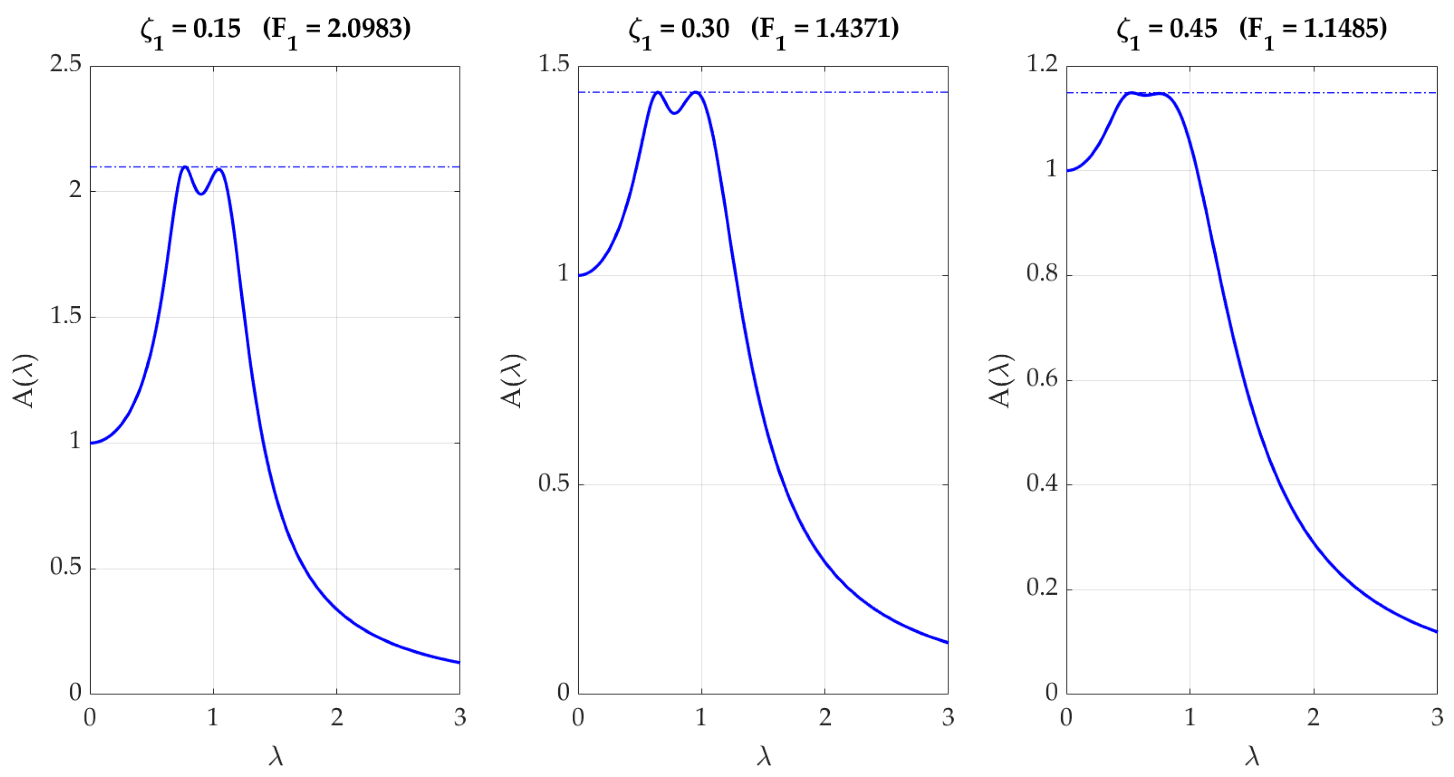
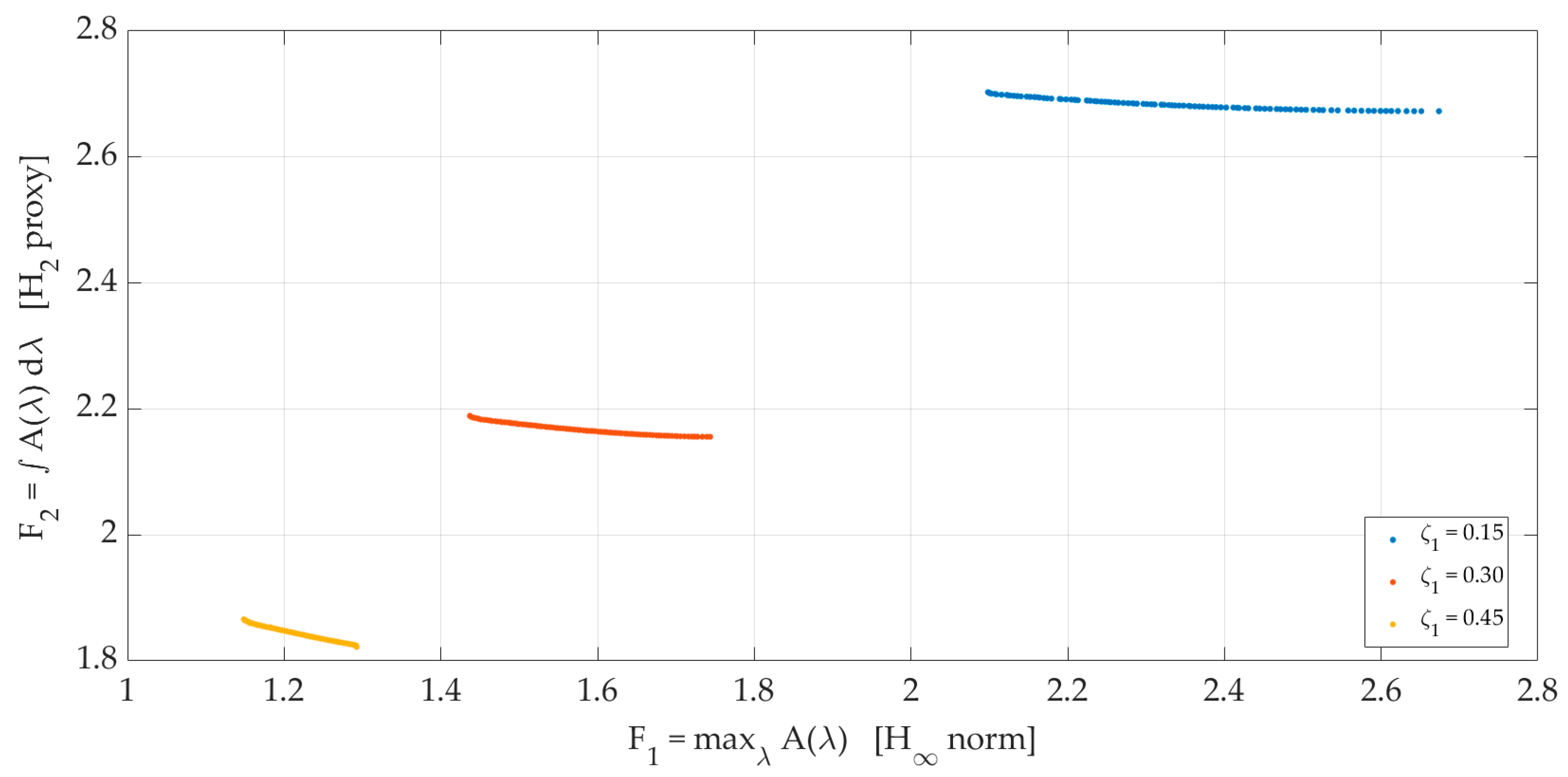
The same procedure has been conducted on the TEDVA problem at three primary damping ratios ${\xi }_1=0.15,0.3$ and $0.45$ with the mass ratio held fixed at $\mu =0.1$.

Table 12. Optimal design of TEDVA across 3 distinct primary damping ratios.

${\mathit{\xi }}_1$	$\mathit{\alpha }$	$\mathit{\nu }$	${\mathit{\xi }}_2$	${\mathbf{F}}_1$	${\mathbf{F}}_2$
$0.15$	0.7507	1.3275	0.2538	2.1022	2.7008
$0.3$	0.6451	1.6840	0.2687	1.4381	2.1878
$0.45$	0.4247	2.1068	0.4610	1.1472	1.8679

summarizes the results.

The results in Table 12 show that the effect of the primary damping ratio is stronger than that of the mass ratio concluded in Table 11. $F_1$ drops from 2.1022 at ${\xi }_1$ = 0.15 to 1.1472 at ${\xi }_1$ = 0.45, a 45.4% reduction, while $F_2$ drops by 30.8% over the same range. This is physically intuitive as the primary structure dissipates more energy on its own, less is left for the absorber to remove, so the achievable peak response falls regardless of how the DVA is tuned. Figure 12 shows the frequency-response curves at each ${\xi }_1$. In addition, Figure 13 overlays the three Pareto fronts.

4.7. Algorithmic Parameter Sensitivity Analysis

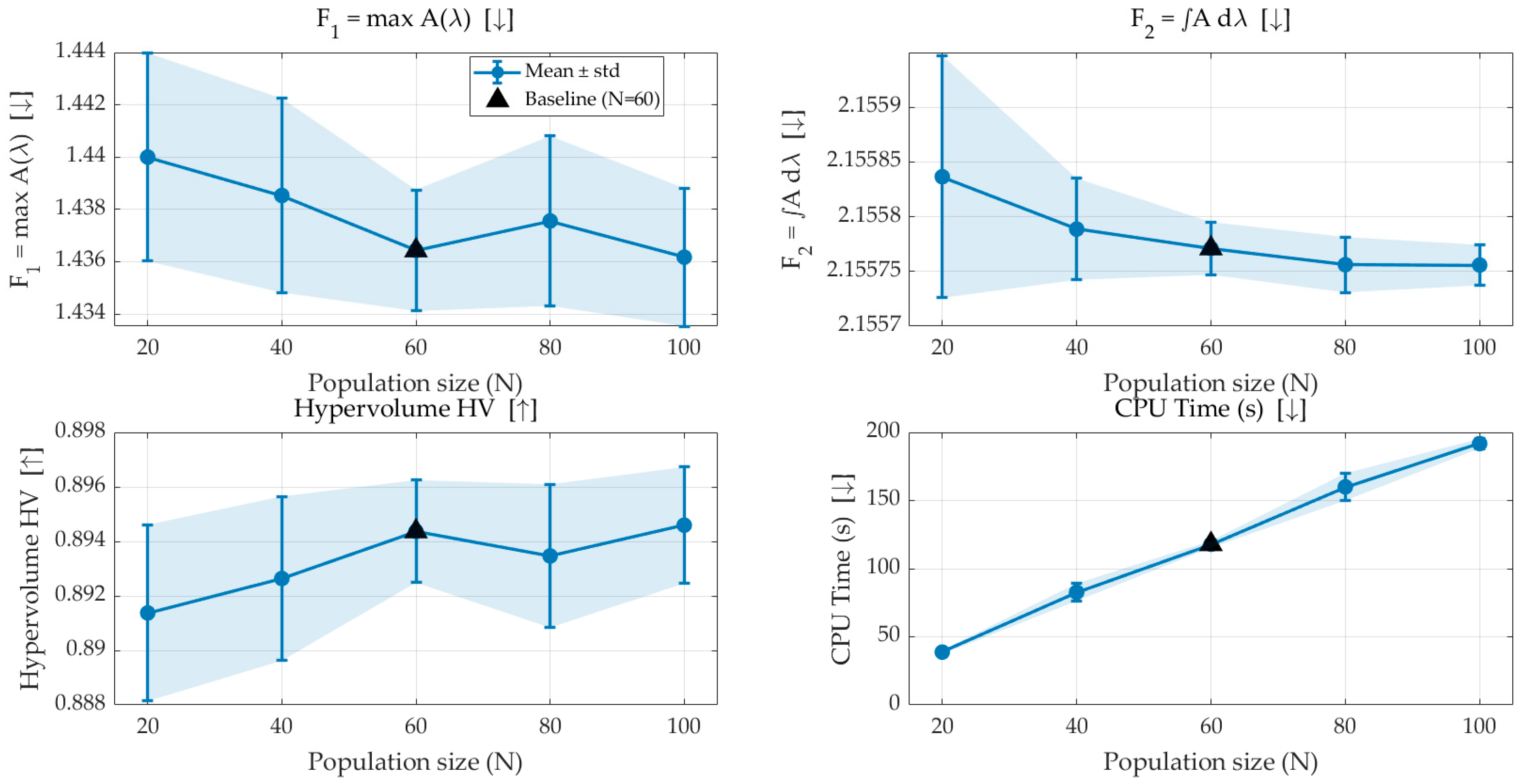
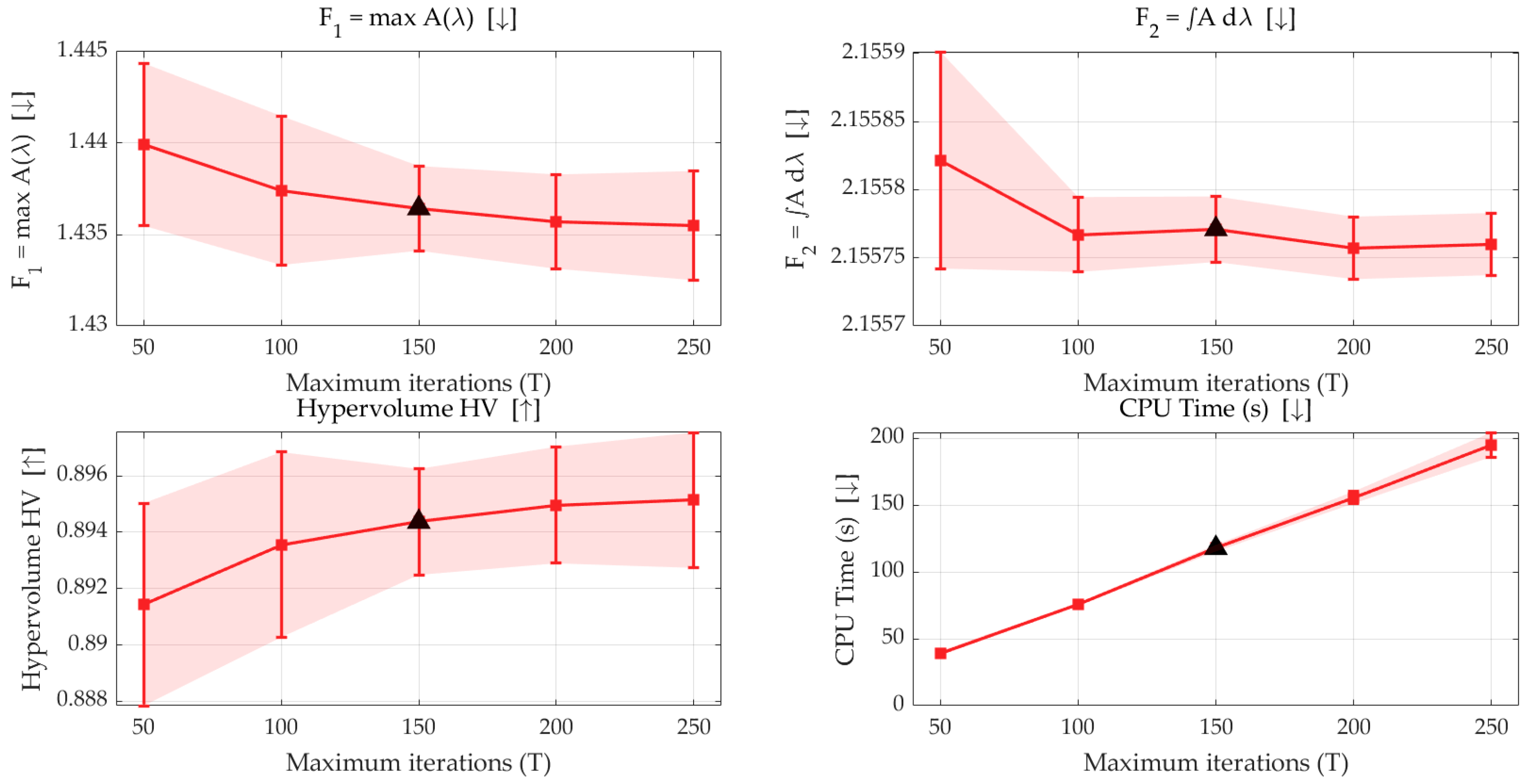
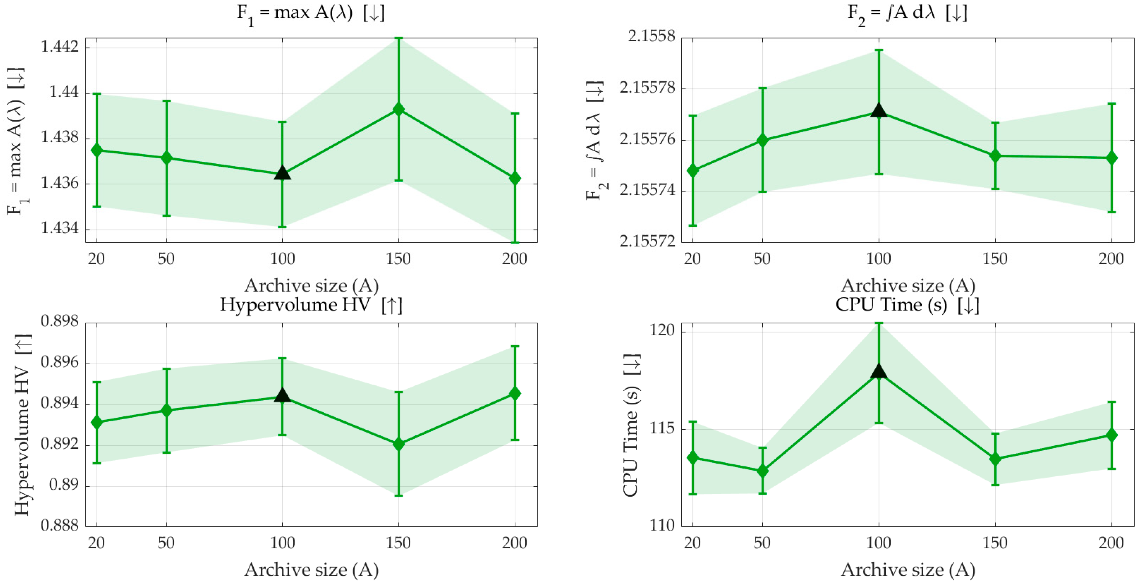
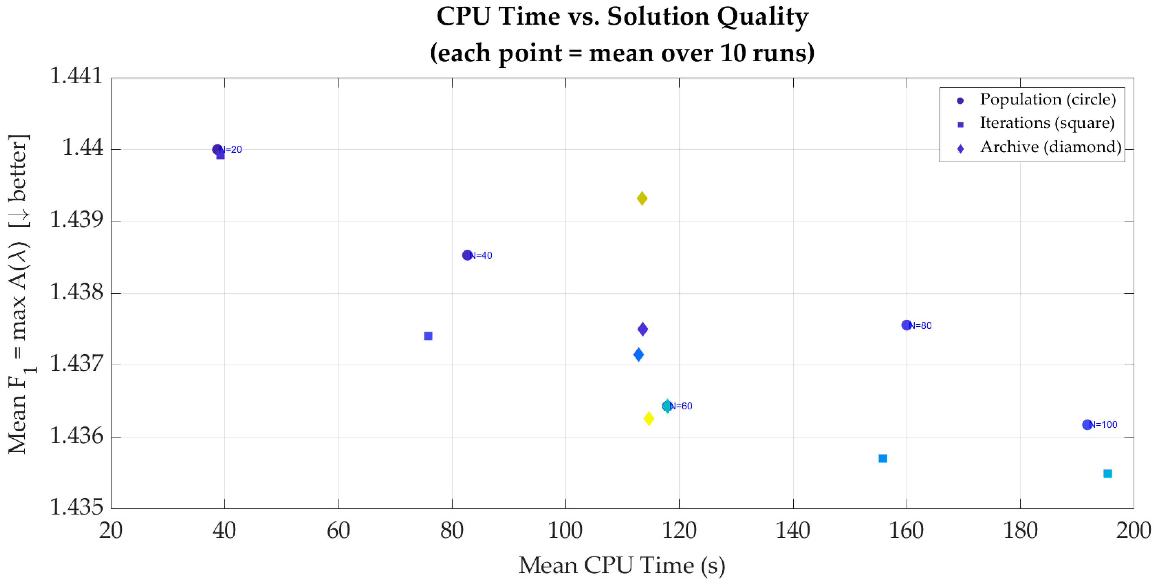
In addition to the physical parameter sensitivity discussed in Section 4.6, the robustness of MODCGJO to its own control parameters—population size ($N$), maximum number of iterations ($T$), and archive size ($A_{\mathrm{m}\mathrm{a}\mathrm{x}}$)—was investigated. A one-at-a-time (OAT) design was used, in which each parameter was varied individually while the other two were held fixed at their baseline values ($N=60, T=150, A_{\mathrm{m}\mathrm{a}\mathrm{x}}=100$). The baseline value of T = 150 was selected as the central, evenly spaced pivot for the iteration sweep (T = 50, 100, 150, 200, 250), allowing symmetric exploration both below and above this point. The number of runs reported in Section 4.1 and Table 5 used T = 200, informed in part by the diminishing-returns trend identified in this sensitivity analysis, which showed that solution quality improves only marginally beyond T ≈ 150–200 while CPU time continues to scale linearly. A slightly higher iteration count (T = 200) was therefore retained for the main results as a conservative margin to ensure full convergence, even though the sensitivity analysis itself confirms this choice is not critical to solution quality. For every configuration, 10 independent runs were performed with different random seeds, and the mean and standard deviation of the peak amplitude ($F_1$), integrated response ($F_2$), Pareto-front size, hypervolume (HV), and CPU time were recorded. The results are summarized in

Table 13. Sensitivity of MODCGJO to algorithm control parameters (10 independent runs per configuration).

Factor	Level	${\mathit{F}}_1$ Mean $\pm$ Std	${\mathit{F}}_2$ Mean $\pm$ Std	PF Size	HV Mean $\pm$ Std	CPU (s) Mean $\pm$ Std
Population	20	1.4400 ± 0.0040	2.1558 ± 0.0001	100	0.8914 ± 0.0032	38.7 ± 1.4
Population	40	1.4385 ± 0.0037	2.1558 ± 0.0001	100	0.8926 ± 0.0030	82.7 ± 6.4
Population	60	1.4364 ± 0.0023	2.1558 ± 0.0000	100	0.8944 ± 0.0019	117.9 ± 2.6
Population	80	1.4376 ± 0.0032	2.1558 ± 0.0000	100	0.8935 ± 0.0026	160.0 ± 10.0
Population	100	1.4362 ± 0.0026	2.1558 ± 0.0000	100	0.8946 ± 0.0021	191.8 ± 3.5
Iteration	50	1.4399 ± 0.0044	2.1558 ± 0.0001	100	0.8914 ± 0.0036	39.3 ± 1.8
Iteration	100	1.4374 ± 0.0041	2.1558 ± 0.0000	100	0.8936 ± 0.0033	75.9 ± 1.2
Iteration	200	1.4357 ± 0.0026	2.1558 ± 0.0000	100	0.8950 ± 0.0021	155.8 ± 4.5
Iteration	250	1.4355 ± 0.0030	2.1558 ± 0.0000	100	0.8951 ± 0.0024	195.3 ± 9.2
Archive	20	1.4375 ± 0.0025	2.1557 ± 0.0000	20	0.8931 ± 0.0020	113.5 ± 1.9
Archive	50	1.4371 ± 0.0025	2.1558 ± 0.0000	50	0.8937 ± 0.0021	112.9 ± 1.2
Archive	150	1.4393 ± 0.0031	2.1558 ± 0.0000	150	0.8921 ± 0.0025	113.5 ± 1.3
Archive	200	1.4363 ± 0.0028	2.1558 ± 0.0000	200	0.8945 ± 0.0023	114.7 ± 1.7

and Figure 14, Figure 15, Figure 16, Figure 17 and Figure 18.

Population size. Figure 14 shows the effect of varying $N$ from 20 to 100 ($T=150, A_{\mathrm{m}\mathrm{a}\mathrm{x}}=100$ fixed). $F_1$ improves from a mean of 1.4400 at $N=20$ to 1.4364 at the baseline $N=60$, with only marginal further improvement at $N=80$ and $N=100$ (1.4376 and 1.4362, respectively). $F_2$ and Pareto-front size remain essentially unchanged across the sweep. CPU time, in contrast, scales approximately linearly with $N$, rising from 38.7 s at $N=20$ to 191.8 s at $N=100$. This indicates diminishing returns in solution quality beyond $N=60$, making it a reasonable efficiency–quality trade-off.

Maximum iterations. Figure 15 shows the corresponding sweep over $T=$ 50–250 ($N=60, A_{\mathrm{m}\mathrm{a}\mathrm{x}}=100$ fixed). $F_1$ decreases monotonically with more iterations, from 1.4399 at $T=50$ to 1.4355 at $T=250$, with the largest gains occurring between $T=50$ and $T=150$ and only marginal improvement thereafter. As with population size, CPU time scales linearly with T (39.3 s at T=50 to 195.3 s at T = 250), while $F_2$ and Pareto-front size remain stable.

Archive size. Figure 16 (archive sweep) shows $F_1$, $F_2$, HV, and CPU time for $A_{\mathrm{m}\mathrm{a}\mathrm{x}}=$ 20−200 ($N=60, T=150$ fixed). Unlike population and iteration count, archive size has negligible effect on CPU time (113–115 s across all values), since it governs only the non-dominated solution storage, not the search cost. $F_1$ shows a mild non-monotonic variation (1.4363–1.4393), attributable to run-to-run noise rather than a systematic trend, and the Pareto-front size scales directly with $A_{\mathrm{m}\mathrm{a}\mathrm{x}},$ as expected, since it caps the number of retained solutions.

CPU time vs. solution quality. Figure 17 (Mean $F_1$ vs. Mean CPU Time) visualizes the trade-off across all three sweeps simultaneously. Population and iteration sweeps show the clearest trade-off pattern, with quality improving steadily as CPU time increases, before flattening out. Archive-size variation, by contrast, clusters tightly around a fixed CPU cost (~113–115 s) with only minor quality variation, confirming that archive size is primarily a memory/diversity parameter rather than a computational-cost driver.

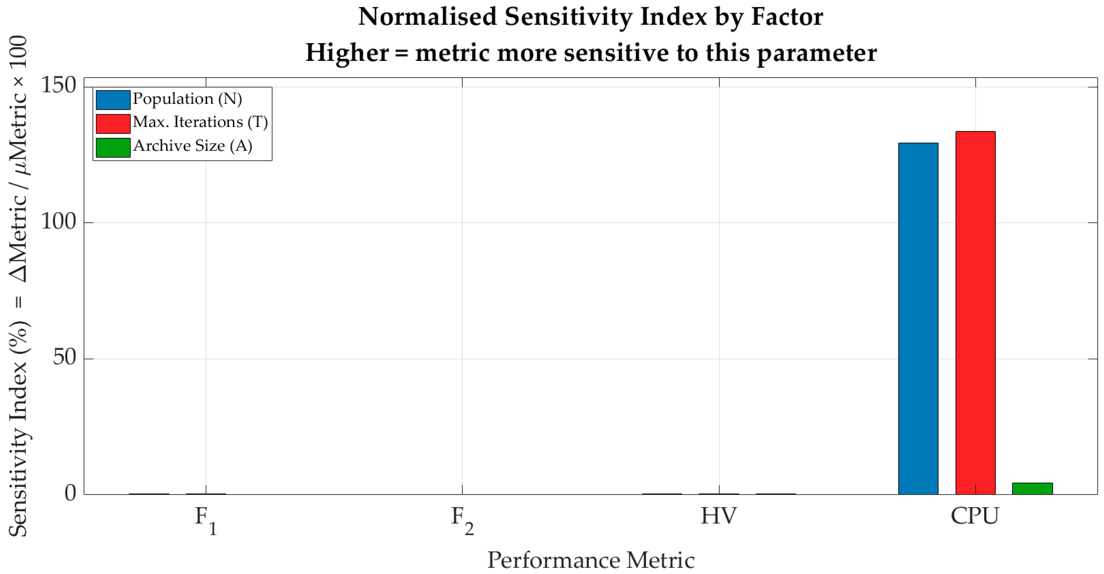
Normalized sensitivity index. Figure 18 quantifies the relative sensitivity of each performance metric to each control parameter, computed as $\Delta Metric/\mu Metric \times 100$. $F_1$, $F_2$, and HV all show sensitivity indices that are below roughly 1% for all three parameters, confirming that solution quality is essentially insensitive to the choice of $N, T$, or $A_{\mathrm{m}\mathrm{a}\mathrm{x}}$ within the tested ranges. CPU time, by contrast, shows a high sensitivity to both population size (≈131%) and maximum iterations (≈135%), and a much smaller sensitivity to archive size (≈5%), consistent with the linear-vs-flat CPU trends observed in Figure 14, Figure 15 and Figure 16.

HV in Table 13 is computed using a fixed reference point [2.5, 3.0], independent of each run’s own Pareto front, and is not normalized—unlike the HV reported in Table 10, which uses an adaptive reference point (1.1 × nadir) normalized to the ideal–reference box. The two are not on the same numerical scale and should not be compared directly; HV in this table is included only to illustrate its relative trend across parameter settings, which remains flat and consistent with the $F_1$/$F_2$/PF-size findings above.

Overall, these results indicate that MODCGJO’s solution quality is robust to the choice of population size, iteration count, and archive size across the ranges tested, while computational cost scales predictably with population size and iteration count and is largely insensitive to archive size. This supports the parameter values adopted for the main experiments (Section 4.1) as a reasonable balance between solution quality and computational cost.

5. Discussion

The superior performance of MODCGJO over the single-objective AM-PSO, together with its competitive performance against the established multi-objective algorithms NSGA-II and MOPSO, can be attributed to several algorithmic innovations:

• Chaotic Initialization: By replacing random initialization with chaotic maps, MODCGJO ensures that the initial population is more uniformly distributed across the search space. This reduces the risk of premature convergence and allows the algorithm to explore promising regions more effectively.
• Pareto Archive with Crowding Distance: The archive mechanism preserves a diverse set of non-dominated solutions, preventing the algorithm from converging to a single point. This is particularly important for multi-objective problems, where maintaining diversity is essential for obtaining a well-distributed Pareto front.
• Crowding-Distance Leader Selection: By selecting leaders from sparse regions of the Pareto front, MODCGJO actively explores under-represented areas. This contrasts with AM-PSO, which is single-objective and focuses only on the best solution.
• DE Mutation with Pareto Acceptance: The DE mutation operator introduces additional diversity, helping the algorithm escape local optima. The Pareto-acceptance criterion ensures that only quality improvements are accepted, maintaining convergence.

Beyond the comparisons against AM-PSO, NSGA-II, and MOPSO, the sensitivity analyses in Section 4.6 and Section 4.7 provide two further layers of confidence in the reported optimum. At the system level, repeating the optimization across four mass ratios ($\mu = 0.05–0.20$) and three primary damping ratios (${\xi }_1 = 0.15–0.45$) shows that both objectives improve monotonically as either parameter increases—$F_1$ falls by 12.1% over the tested mass-ratio range and by 45.4% over the tested damping-ratio range—while the optimal design variables ($\alpha , \nu , {\xi }_2$) shift in a physically coherent, monotonic direction. This confirms that the reported optimum is not an artifact of the single ($\mu = 0.1, {\xi }_1= 0.3$) case study adopted from Song et al. [1] but generalizes across realistic host-structure conditions. At the algorithmic level, varying MODCGJO’s own control parameters—population size, iteration count, and archive size—over wide ranges changes solution quality ($F_1, F_2,$ hypervolume) by less than 1%, while computational cost scales predictably with population size and iteration count and is nearly insensitive to archive size. This indicates that MODCGJO’s performance does not depend on delicate parameter tuning, and that the settings adopted for the main experiments ($N = 60, T = 200, A_{max} = 100$) represent a reasonable, non-critical point on the quality–cost trade-off curve.

The Pareto front generated by MODCGJO provides engineers with flexible design choices. Depending on the application requirements, one can select:

• A low-peak design (left side of the front) for applications where worst-case vibration is critical (e.g., precision machinery, sensitive equipment).
• A low-energy design (right side of the front) for applications where broadband vibration is more important (e.g., comfort in vehicles, noise reduction).
• A balanced design (middle of the front) for general-purpose applications.
• This flexibility is a key advantage over single-objective methods, which provide only a single solution.

The value of MODCGJO to a practicing engineer lies not in a single optimized design point, but in the Pareto front itself, which converts the $H_{\infty }$/$H_2$ trade-off into an explicit design decision. We outline both the application workflow and the physical realization of a selected design.

Application workflow: (1) The primary structure’s mass $m_1$, stiffness $k_1$, and damping ratio ${\zeta }_1$ are obtained from modal testing or design specifications of the structure to be protected (e.g., a machine base, building floor, or vehicle subframe). (2) The absorber mass ratio $\mu$ is fixed according to the maximum added mass the application can tolerate—small for weight-sensitive applications (aerospace, precision instruments), and larger for civil structures. (3) MODCGJO is run with $m_1$, $k_1$, ${\zeta }_1$, $\mu$ fixed, returning a set of non-dominated $\left(\alpha ,\nu ,{\zeta }_2\right)$ designs spanning the peak-amplitude ($F_1$) vs. broadband-energy ($F_2$) trade-off. (4) The engineer selects an operating point based on the excitation environment: near-resonance/narrowband excitation (e.g., rotating machinery at fixed speed) favors an $F_1$-optimal design, while broadband/random excitation (e.g., road- or wind-induced vibration) favors an $F_2$-optimal design—a judgment call the front informs but does not make automatically. (5) The selected design is converted to physical components and validated experimentally.

Given the primary structure’s known properties, any selected point on the front converts directly to physical component values via $k_2=\mu {\alpha }^2{k}_1$, $k_3=\nu k_2$, $c_2=2{\zeta }_2\mu \alpha \sqrt{k_1{m}_1}$—the same conversion applies regardless of which point on the front is chosen, so the multi-objective output does not complicate the realization step, only the selection step.

Engineering challenges: (i) The idealized massless internal node $x_3$ requires the physical linkage between $k_3$ and $c_2$ to have negligible mass relative to $m_1,m_2$; a non-negligible linkage mass introduces a parasitic high-frequency resonance not captured by the present model. (ii) Real components exhibit amplitude, temperature, and frequency-dependent stiffness and damping—particularly for elastomeric realizations—which can mistune the absorber from its optimized point, motivating the robustness checks already performed across mass ratio and primary damping in Section 4.6, though component-level manufacturing tolerance was not modeled directly. (iii) The absorber mass fraction ($\mu =0.1$ in the case study) represents a real added-weight constraint in weight-sensitive applications. (iv) Achieving the precise, continuously tunable damping required is nontrivial with standard passive dampers; a semi-active realization of $c_2$ using a magnetorheological or electrorheological damper would allow post-installation retuning to compensate for manufacturing variance or drift, at added cost and complexity.

The 7.3% reduction in peak amplitude achieved by MODCGJO translates to:

• Improved reliability: Reduced vibration amplitudes extend the fatigue life of structural components.
• Enhanced performance: Lower peak response improves the accuracy of precision systems.
• Cost savings: Passive absorbers are simpler and cheaper than active control systems; optimizing their design maximizes their effectiveness.

Beyond these single-objective gains, the close agreement between MODCGJO, NSGA-II, and MOPSO (Section 4.3) indicates that a practicing engineer can adopt MODCGJO’s Pareto front with confidence that it reflects the true trade-off surface, rather than an artifact of a single algorithm’s search bias.

While MODCGJO demonstrates excellent performance, it has some limitations:

• Computational cost: The archive management (non-dominated sorting and crowding distance) adds computational overhead compared to single-objective GJO and DE mutation steps introduce additional fitness evaluations per iteration (Section 3.2.6). As derived in Section 3.2.6, MODCGJO’s per-iteration cost is comparable to NSGA-II’s in the dominant fitness-evaluation term, but its repeated re-computation of crowding-distance truncation is less efficient than NSGA-II’s one-shot computation, which may become a bottleneck for large archive sizes ($A\gg A_{max}$). However, for the TEDVA problem (500 frequency points, 60 agents, 200 iterations), the total runtime is approximately 157 s, which is acceptable for engineering design and consistent with the results of the algorithm’s sensitivity analysis conducted in Table 13, but has not been benchmarked for real-time or embedded use.
• Parameter tuning: MODCGJO introduces additional parameters ($p_{DE}$, $F$, $CR$, $A_{\mathrm{m}\mathrm{a}\mathrm{x}}$). While these were set based on literature recommendations, a systematic parameter sensitivity study could further optimize performance.
• Generalization: While Section 4.6.2 confirms that the optimum generalizes across a realistic range of mass ratios and primary damping values, the present study is still limited to the TEDVA topology itself. Future work could extend the approach to other DVA topologies (e.g., with inerter or negative stiffness) or other engineering optimization problems like [2,29,30].

6. Conclusions

This paper has presented a comprehensive investigation into the multi-objective optimization of the three-element dynamic vibration absorber (TEDVA) using the proposed Multi-Objective Chaotic Golden Jackal Optimization (MODCGJO). A robust mathematical model was developed using a direct matrix formulation of the TEDVA frequency response by solving the full 3 × 3 complex dynamic stiffness system, avoiding the numerical cancelation and normalization errors that plague closed-form polynomial expressions. The MODCGJO algorithm was proposed by extending the standard Golden Jackal Optimization with four key innovations: dynamic chaotic map-based initialization, a Pareto-dominance archive with crowding-distance truncation, crowding-distance-based leader selection, and a self-adaptive differential evolution mutation operator with Pareto-acceptance. Applied to the TEDVA problem with fixed parameters $\mu = 0.1$ and ${\xi }_1 = 0.3$, MODCGJO successfully generated a high-quality Pareto front of 100 non-dominated solutions. The best $H_{\infty }$ solution ($\alpha = 0.6487, \nu = 1.7778, {\xi }_2= 0.2657$) achieved a peak amplitude of $F_1 = 1.4395$, representing a 7.3% reduction compared to the state-of-the-art AM-PSO TEDVA solution (F₁ = 1.5535) and a 32.3% reduction compared to the Voigt DVA (F₁ = 2.1249), while maintaining a competitive $H_2$ performance ($F_2 = 2.1873$). Benchmarking against the established multi-objective algorithms NSGA-II and MOPSO under identical conditions produced nearly overlapping Pareto fronts (differences within 0.3%), confirming that MODCGJO is a competitive, well-validated multi-objective optimizer rather than an artifact of a single algorithm’s search bias. Pareto quality metrics confirmed the excellence of the obtained front: normalized Hypervolume (0.9717), Generational Distance ($1.69 \times {10}^{-4}$), Inverted Generational Distance ($1.06 \times {10}^{-3}$), Spacing ($9.48 \times {10}^{-4}$), and Spread (0.253). Sensitivity analyses revealed that the optimal spring ratio ($\nu = 1.7778$) and damping ratio (${\xi }_2 = 0.2657$) provide the best balance between the two anti-resonance dips, effectively flattening the frequency response. System-level sensitivity analysis further confirmed that this optimum generalizes across a realistic range of host-structure conditions, with both objectives improving monotonically as mass ratio (12.1% reduction in $F_1$ over $\mu = 0.05-0.20$) and primary damping (45.4% reduction in $F_1$ over ${\xi }_1 = 0.15-0.45$) increase, while the optimal design parameters shift in a physically coherent manner. Algorithmic sensitivity analysis showed that MODCGJO’s solution quality is robust (less than 1% variation) to its own control parameters—population size, iteration count, and archive size—confirming that the algorithm does not require delicate tuning to perform reliably. The Pareto front provides engineers with flexible design options, enabling them to select the optimal trade-off between peak suppression and broadband energy reduction based on specific application requirements. Future work will extend the approach to other DVA topologies (e.g., with an inerter or negative stiffness), investigate real-time or embedded-hardware feasibility, and pursue experimental validation of the optimal designs.

References

1. Song, Q.H.; Xiao, L.J.; Song, Q.J.; Jiang, H.Y.; Liu, X.J. Adaptive multiswarm particle swarm optimization for tuning the parameter optimization of a three-element dynamic vibration absorber. Mech. Sci. 2022, 13, 505–517. [Google Scholar] [CrossRef] [Scilit]
2. Frahm, H. Device for Damping Vibrations of Bodies. U.S. Patent No. 989,958, 18 April 1911. [Google Scholar]
3. Gao, T.; Li, J.; Zhu, S.; Yang, X.; Zhao, H. H∞ optimization of three-element-type dynamic vibration absorber with inerter and negative stiffness based on the particle swarm algorithm. Entropy 2023, 25, 1048. [Google Scholar] [CrossRef] [Scilit] [PubMed]
4. Ormondroyd, J.; Den Hartog, J.P. The theory of the dynamic vibration absorber. Trans. ASME 1928, 49, 021007. [Google Scholar] [CrossRef] [Scilit]
5. Asami, T.; Nishihara, O. Analytical and experimental evaluation of an air damped dynamic vibration absorber: Design optimizations of the three-element type model. J. Vib. Acoust. 1999, 121, 334–342. [Google Scholar] [CrossRef] [Scilit]
6. Asami, T.; Nishihara, O. H2 optimization of the three-element type dynamic vibration absorbers. J. Vib. Acoust. 2002, 124, 583–592. [Google Scholar] [CrossRef] [Scilit]
7. Den Hartog, J.P. Mechanical Vibrations; Courier Corporation: North Chelmsford, MA, USA, 1985. [Google Scholar]
8. Nishihara, O. Exact optimization of a three-element dynamic vibration absorber: Minimization of the maximum amplitude magnification factor. J. Vib. Acoust. 2019, 141, 011001. [Google Scholar] [CrossRef] [Scilit]
9. Esen, I.; Koç, M.A. Optimization of a passive vibration absorber for a barrel using the genetic algorithm. Expert Syst. Appl. 2015, 42, 894–905. [Google Scholar] [CrossRef] [Scilit]
10. Xie, S.; Li, P.; Zhang, X.; Yan, B. Vibration suppression of structure with electromagnetic shunt damping absorber. Int. J. Appl. Electromagn. Mech. 2014, 45, 395–402. [Google Scholar] [CrossRef] [Scilit]
11. Liu, M.; Gu, F.; Huang, J.; Wang, C.; Cao, M. Integration design and optimization control of a dynamic vibration absorber for electric wheels with in-wheel motor. Energies 2017, 10, 2069. [Google Scholar] [CrossRef] [Scilit]
12. Cui, Y.; Li, J.; Yu, Y.; Jiang, R. Vibration control and parameter optimization of a dynamic vibration absorber with inerter and negative stiffness. J. Phys. Conf. Ser. 2025, 3145, 012036. [Google Scholar] [CrossRef] [Scilit]
13. Costa, P.D.O.B.D.; Miguel, L.F. Optimization of inerter-based dynamic vibration absorbers for vibration control in buildings subjected to seismic excitations. Shock Vib. 2025, 2025, 5280674. [Google Scholar] [CrossRef] [Scilit]
14. Cui, Y.; Li, J.; Zhu, S.; Gao, T. Performance analysis and parameter optimization of an inerter-based vibration absorber with negative stiffness and parallel configuration. J. Nonlinear Math. Phys. 2026, 33, 17. [Google Scholar] [CrossRef] [Scilit]
15. Shamseldin, A.; Abido, M.A.; Alofi, A. AI-driven optimization of dynamic vibration absorbers with hydraulic amplifier and mechanical inerter integration. Front. Mech. Eng. 2024, 10, 1464692. [Google Scholar] [CrossRef] [Scilit]
16. Zhang, K.; Wang, S.; Wu, J.; Zheng, C.; Bi, C. Robust optimization of dynamic vibration absorber array for vibration attenuation of mistuned bladed disk. J. Vib. Acoust. 2026, 148, 011002. [Google Scholar] [CrossRef] [Scilit]
17. Snowdon, J.C. Dynamic vibration absorbers that have increased effectiveness. J. Eng. Ind. 1974, 96, 940–945. [Google Scholar] [CrossRef] [Scilit]
18. Chopra, N.; Ansari, M.M. Golden jackal optimization: A novel nature-inspired optimizer for engineering applications. Expert Syst. Appl. 2022, 198, 116924. [Google Scholar] [CrossRef] [Scilit]
19. Rizk-Allah, R.M.; Hassanien, A.E.; Bhattacharyya, S. Chaotic crow search algorithm for fractional optimization problems. Appl. Soft Comput. 2018, 71, 1161–1175. [Google Scholar] [CrossRef] [Scilit]
20. El-henawy, I.; Abdel-Raouf, O.; Abdelbaset, M. Improved harmony search algorithm with chaos for solving definite integral. Int. J. Oper. Res. 2014, 21, 252–261. [Google Scholar] [CrossRef] [Scilit]
21. Chuang, L.Y.; Tsai, S.W.; Yang, C.H. Chaotic catfish particle swarm optimization for solving global numerical optimization problems. Appl. Math. Comput. 2011, 217, 6900–6916. [Google Scholar] [CrossRef] [Scilit]
22. Caponetto, R.; Fortuna, L.; Fazzino, S.; Xibilia, M.G. Chaotic sequences to improve the performance of evolutionary algorithms. IEEE Trans. Evol. Comput. 2003, 7, 289–304. [Google Scholar] [CrossRef] [Scilit]
23. Kuang, F.; Jin, Z.; Xu, W.; Zhang, S. A novel chaotic artificial bee colony algorithm based on tent map. In Proceedings of the 2014 IEEE Congress on Evolutionary Computation (CEC), Beijing, China, 6–11 July 2014; pp. 235–241. [Google Scholar] [CrossRef] [Scilit]
24. Metwalli, M.; Abdel-baset, M.; Hezam, I. A modified flower pollination algorithm for fractional programming problems. Int. J. Intell. Syst. Appl. Eng. 2015, 3, 116–123. [Google Scholar] [CrossRef] [Scilit]
25. Deb, K.; Pratap, A.; Agarwal, S.; Meyarivan, T. A fast and elitist multiobjective genetic algorithm: NSGA-II. IEEE Trans. Evol. Comput. 2002, 6, 182–197. [Google Scholar] [CrossRef] [Scilit]
26. Storn, R.; Price, K. Differential evolution—A simple and efficient heuristic for global optimization over continuous spaces. J. Glob. Optim. 1997, 11, 341–359. [Google Scholar] [CrossRef] [Scilit]
27. Coello, C.A.C.; Pulido, G.T.; Lechuga, M.S. Handling multiple objectives with particle swarm optimization. IEEE Trans. Evol. Comput. 2004, 8, 256–279. [Google Scholar] [CrossRef] [Scilit]
28. Mirjalili, S.; Saremi, S.; Mirjalili, S.M.; Coelho, L.D.S. Multi-objective grey wolf optimizer: A novel algorithm for multi-criterion optimization. Expert Syst. Appl. 2016, 47, 106–119. [Google Scholar] [CrossRef] [Scilit]
29. Li, J.; Sun, Y.; Liu, X.; Zhang, Y. Tuning Mechanism and Parameter Optimization of a Dynamic Vibration Absorber with Inerter and Negative Stiffness under Delayed FOPID. Mathematics 2025, 13, 2124. [Google Scholar] [CrossRef] [Scilit]
30. Chen, Y.; Li, J.; Zhu, S.; Zhao, H. Further optimization of Maxwell-type dynamic vibration absorber with inerter and negative stiffness spring using particle swarm algorithm. Mathematics 2023, 11, 1904. [Google Scholar] [CrossRef] [Scilit]
Figure 1. The main structure of Voigt DVA and TEDVA.
Mca 31 00149 g001
Figure 2. Free body diagram of the TEDVA system.
Mca 31 00149 g002
Figure 3. MODCGJO flow chart.
Mca 31 00149 g003
Figure 4. TEDVA pareto front obtained by MODCGJO vs. single-objective results of AM-PSO.
Mca 31 00149 g004
Figure 5. TEDVA pareto front H vs. H 2 for MODCGJO vs. NSGA-II vs. MOPSO.
Mca 31 00149 g005
Figure 6. Frequency response comparison between MODCGJO vs. AM-PSO.
Mca 31 00149 g006
Figure 7. Frequency response comparison of the best H -optimal solutions obtained by MODCGJO, NSGA-II, MOPSO.
Mca 31 00149 g007
Figure 8. Effect of spring ratio on frequency response.
Mca 31 00149 g008
Figure 9. Effect of damping ratio on frequency response.
Mca 31 00149 g009
Figure 10. Frequency response comparison for distinct four mass ratio values.
Mca 31 00149 g010
Figure 11. Pareto frontiers obtained for distinct four mass ratio values.
Mca 31 00149 g011
Figure 12. Frequency response comparison for three distinct primary damping ratios.
Mca 31 00149 g012
Figure 13. Pareto frontiers obtained across distinct three primary damping ratios.
Mca 31 00149 g013
Figure 14. Effect of population size (N) on F1, F2, hypervolume, and CPU time.
Mca 31 00149 g014
Figure 15. Effect of number of iterations (T) on F1, F2, hypervolume, and CPU time.
Mca 31 00149 g015
Figure 16. Effect of archive size (A) on F1, F2, hypervolume, and CPU time.
Mca 31 00149 g016
Figure 17. Mean F1 versus mean CPU time across all population, iteration, and archive-size configurations.
Mca 31 00149 g017
Figure 18. Normalized sensitivity index.
Mca 31 00149 g018