Numerical Approximation of a Smoking Dynamics Model Using a Hybrid Deep Neural Network Architecture

Abstract

Despite the fact that smoking is still a significant global public health concern, current mathematical models of smoking dynamics primarily depend on conventional numerical solvers. A particular five-compartment smoking dynamics model has not yet been solved using deep neural network (DNN) techniques. In order to fill this research gap, this work creates a unique DNN framework that can simulate nonlinear smoking dynamics in a computationally efficient manner. The Levenberg–Marquardt backpropagation technique is used to improve a dual-hidden-layer network consisting of 20 radial basis activation function (RBAF) neurons and 40 log-sigmoid activation function (LSAF) neurons. With a minimum mean squared error (MSE) of $1.865\times {10}^{-6}$ and a coefficient of determination $R^2$ equal to or near unity across all model variables, the trained DNN offers instantaneous predictions while maintaining superior accuracy, in contrast to traditional numerical methods that necessitate the explicit re-solving of differential equations for each parameter change. Crucially, our DNN-based framework is appropriate for automated public health decision-support systems since it functions independently and does not require human intervention during the prediction phase. Key smoking behaviors, such as initiation, quitting efforts, relapse dynamics, and long-term recovery patterns, are successfully replicated by the framework, while relapse dynamics are captured through the recovered-to-potential smoker pathway, consistent with the original model formulation. These findings show that the proposed DNN approach not only closes the methodological gap in the application of deep learning to smoking dynamics but also offers a dependable and computationally effective tool for quick evaluation of intervention scenarios, supporting evidence-based public health decision making without compromising accuracy.

1. Introduction

One of the most significant worldwide public health problems is still smoking, resulting in millions of avoidable deaths every year. The World Health Organization estimates that tobacco use, including both direct smokers and those exposed to secondhand smoke, causes about 8 million deaths annually [1]. The health consequences of smoking include various cancers, cardiovascular diseases, respiratory illnesses, and reduced life expectancy. Smoking cessation models are crucial to understanding the dynamics of smoking behavior and developing effective public health interventions [2].

Biologists depend significantly on the use of mathematics, as mathematical modeling plays an essential role in the analysis of biological systems [3,4]. Mathematical models in epidemiology help researchers understand disease transmission patterns, predict outbreaks, and evaluate intervention strategies [5]. In the context of smoking behavior, compartmental models have been widely used to study the transitions between different smoking statuses within populations [6]. In order to analyze the dynamics of smoking initiation, cessation, and relapse, these models usually classify people into categories such as potential smokers, current smokers, former smokers, and quitters.

The architecture of biological neural networks is the source of neural networks (NNs). For complex computations and pattern recognition applications, the NN design is crucial. An NN uses interconnected processing units called neurons to combine several responses to produce output. The capacity to generate precise predictions and classifications is improved by NNs [7]. These basic processing components are linked into a network in several layers to form DNNs. These processing centers are unique in that they function as many levels of abstraction rather than being fixed by design. A layer of input and a layer of output make up a single-layer NN. The models are commonly referred to as DNNs when more layers are added [8].

Despite several public health initiatives, tobacco smoking still has a significant global burden. Approximately 22.3% of people worldwide used tobacco in 2020; the incidence was higher in low- and middle-income nations [9]. Peer pressure, societal circumstances, and genetic predispositions all play important roles in influencing smoking behavior, which usually starts during adolescence [10]. Once established, nicotine dependence makes quitting smoking difficult, with relapse being a significant challenge in smoking cessation efforts [11]. Pharmacological treatments, behavioral therapy, and public health measures like tobacco taxes and smoking bans have all been created as interventions to help people quit smoking [12].

ANNs can forecast outcomes by learning from provided data. They are crucial to managing a large number of disorganized data. ANNs are capable of data handling, numerical control, forecasting, time-series analysis, function approximation, and computational processing, among other tasks [13]. Consequently, a DNN can approximate many natural functions with fewer components by leveraging the function’s structure [14]. NN-based stochastic numerical assessments assess the precision of differential equation (DE) solutions in a range of applications [15]. In order to assist computers perform tasks that are similar to those that humans perform best, artificial DNNs were first inspired by portions of the brain. DNNs are being used more and more by cognitive scientists to study the brain and neurology, since they lack information on these cognitive processes, which has sparked a lot of debate [16].

In this study, we solve a five-compartment smoking model using an effective DNN approach based on the Levenberg–Marquardt backpropagation (LMB) algorithm, referred to as the DNN-LMB technique. Potential (P), active (S), recovered (R), quitter (Q), and death (D) smokers are all taken into account in this model. We demonstrate that a typical NN with suitable activation functions may correctly approximate the ODE solutions by applying a dual-hidden-layer DNN (RBAF + LSAF) to this smoking dynamics model. A rigorous performance evaluation across several test problems and a comparison with RK4 offer a helpful baseline for future machine learning applications in smoking epidemiology, even if the architecture itself makes use of well-established components.

The DNN technique was favored in this work due to its computational efficiency, rapid convergence, and ability to make precise predictions of nonlinear differential systems, even though there are a number of methods for simulating nonlinear models using artificial intelligence, including Physics-Informed NNs (PINNs), Recurrent NNs and Genetic Algorithms [17]. Recent developments have shown that NN paradigms are useful for analyzing disease dynamics. For example, Waseem et al. [18] used an unsupervised stochastic NN approach to an infectious disease mathematical model, and Ali et al. [19] presented a disease-informed NN framework for optimizing COVID-19 dynamics. We make it clear that the proposed DNN framework’s computational efficiency is not meant to surpass RK4 for a single forward solve; rather, following a single offline training run, the trained network offers instantaneous predictions for multiple parameter sets and initial conditions, which is beneficial for real-time public health intervention modeling where a large number of “what-if” scenarios are assessed. In a variety of scientific fields, DNNs offer effective methods for model training and exceptional accuracy in pattern recognition [20]. Our approach outperforms traditional and certain contemporary AI methods in terms of decrease of errors and speed for small-to-medium-sized datasets by effectively approximating the dynamics of the smoking model through the combination of DNN structure with LMB optimization [21].

Feed-forward backpropagation NNs have been used in many studies to solve difficult problems. This study’s dynamic smoking model models changes in a population’s smoking status. Variations in several parameters, such as smoking start rates, quitting rates, relapse probabilities, and mortality rates, are taken into account in model analysis. The DNN-LMB technique is used to extract numerical results. By comparing the outcomes with those produced by the Runge–Kutta numerical algorithm, accuracy, correctness, and reliability are guaranteed. The rate of convergence of the proposed DNN-LMB technique is assessed using graphical analysis.

Our novelty is the specific layer allocation (20 RBAF + 40 LSAF) optimized via LMB for the five-compartment smoking model, in contrast to generic hybrid RBAF-LSAF architectures in the literature. Comparative experiments demonstrate 62% lower MSE and faster convergence than single-layer RBAF or LSAF configurations.

There are various sections in the present article: Section 2 explains the concept and parameter choices of the smoking dynamics model. Section 3 discusses the use of the DNN technique in conjunction with LSAF and RBAF. Section 4 explains the DNN technique’s convergence and validation. Numerical findings and comparisons with conventional approaches are displayed in Section 5. Section 6 presents the conclusions.

2. Construction of Model

There are five population compartments in the smoking dynamics model under consideration: The total number of smoking-related fatalities over time is represented by the compartment $D\left(t\right)$. It is the part of the model used to track mortality outcomes related to smoking. $P\left(t\right)$ represents potential smokers (individuals susceptible to starting smoking), $S\left(t\right)$ denotes active smokers (individuals currently smoking), $R\left(t\right)$ stands for recovered smokers (who have quit and developed resistance), and $Q\left(t\right)$ represents quitter smokers (who have quit smoking), but it does not contribute to the initiation, cessation, recovery, or relapse processes governing smoking transmission dynamics.

The reference model’s total population accounting framework is represented by $N\left(t\right)=S\left(t\right)+P\left(t\right)+Q\left(t\right)+R\left(t\right)$. The following set of ordinary differential equations describes the smoking model:

$$\left\{\begin{array}{c}{\displaystyle \frac{dP}{dt}}=\mathrm{\Lambda }-{\beta }_{1}PS-(\mu +\varphi +{\beta }_2)P+\alpha (1-ϵ)S+\pi \theta R,\hfill \\ {\displaystyle \frac{dS}{dt}}={\beta }_{1}PS-(\mu +\alpha +\rho +\gamma )S,\hfill \\ {\displaystyle \frac{dR}{dt}}=\alpha ϵS+\rho S-(\mu +\theta )R,\hfill \\ {\displaystyle \frac{dQ}{dt}}={\beta }_{2}P+\varphi P+(1-\pi )\theta R-\mu Q,\hfill \\ {\displaystyle \frac{dD}{dt}}=\gamma S,\hfill \end{array}\right.$$

(1)

with initial conditions (ICs):

$$S\left(0\right)\ge 0,P\left(0\right)\ge 0,Q\left(0\right)\ge 0,R\left(0\right)\ge 0,D\left(0\right)\ge 0.$$

The definitions and values of the smoking model parameters are provided in Table 1.

It should be mentioned that the smoking dynamics model used in this study was taken from Ali et al.’s research work [22] with minor modifications to improve its mathematical consistency. As a result, the original formulation’s epidemiological presumptions and transition mechanisms including relapse dynamics are retained.

Real-world smoking behavior patterns, such as initiation, cessation, relapse, and mortality, are reflected in the parameters that govern the flow dynamics between various smoking states [6]. In order to solve this system numerically and enable the effective modeling and analysis of smoking dynamics under different intervention scenarios, we propose a DNN approach in the following sections.

3. Technique: A Deep Neural Network

While several artificial intelligence techniques, such as Recurrent NNs, Genetic Algorithms, and PINNs, can simulate nonlinear models, the DNN technique was favored in this work due to its high computational efficiency, quick convergence, and capacity to accurately predict nonlinear differential systems. DNNs are effective methods for training a model to identify patterns in a wide range of scientific fields with exceptional accuracy [8,15]. LMB optimization and DNN structure work together to effectively replicate the smoking model’s dynamics, surpassing both traditional and some contemporary AI techniques in terms of training speed and reduction in errors for datasets that are modest-to-medium in size.

A DNN is described as a multi-layered method with input, hidden, and output layers. To compute nonlinear dynamics for the smoking model, the mathematical DNN procedure uses twenty to forty neurons with RBAF and LSAF. In this NN architecture, the activation functions are represented by $f_1$ and $f_2$, with the associated bias vectors and weight matrices for the first, second, and output layers. The first hidden layer utilizes a RBAF, while the second hidden layer employs a LSAF.

$$\left[\begin{array}{c}{u}_1\\ u_2\\ u_3\\ ⋮\\ u_{20}\end{array}\right]=f_1\left(\begin{array}{c}\left[\begin{array}{c}{\eta }_{1,1}\\ {\eta }_{1,2}\\ {\eta }_{1,3}\\ ⋮\\ {\eta }_{1,20}\end{array}\right]\left[x\right]+\left[\begin{array}{c}{b}_{1,1}\\ b_{1,2}\\ b_{1,3}\\ ⋮\\ b_{1,20}\end{array}\right]\end{array}\right)$$

(2)

The architecture begins with the first hidden layer, which processes the single input x and produces 20 hidden outputs. As shown in Equation (2), the weight vector ${\eta }_{1,i}$ and bias $b_{1,i}$ are applied to the input, and the result is passed through the RBAF $f_1$ to produce the outputs $u_i$ (where $i=1,\dots ,20$).

$$\left[\begin{array}{c}{v}_1\\ v_2\\ v_3\\ ⋮\\ v_{40}\end{array}\right]=f_2\left(\left[\begin{array}{ccccc}{\zeta }_{1,1}& {\zeta }_{2,1}& {\zeta }_{3,1}& \dots & {\zeta }_{20,1}\\ {\zeta }_{1,2}& {\zeta }_{2,2}& {\zeta }_{3,2}& \dots & {\zeta }_{20,2}\\ {\zeta }_{1,3}& {\zeta }_{2,3}& {\zeta }_{3,3}& \dots & {\zeta }_{20,3}\\ ⋮& ⋮& ⋮& \ddots & ⋮\\ {\zeta }_{1,40}& {\zeta }_{2,40}& {\zeta }_{3,40}& \dots & {\zeta }_{20,40}\end{array}\right]\left[\begin{array}{c}{u}_1\\ u_2\\ u_3\\ ⋮\\ u_{20}\end{array}\right]+\left[\begin{array}{c}{b}_{2,1}\\ b_{2,2}\\ b_{2,3}\\ ⋮\\ b_{2,40}\end{array}\right]\right)$$

(3)

The second hidden layer, described by Equation (3), takes the 20 outputs from the first layer and expands them to 40 new hidden outputs. Here, the 20 values $u_i$ are linearly combined using the weight matrix ${\zeta }_{i,j}$ (of dimension $40\times 20$) and added to the bias vector ${\mathbf{b}}_2$ (of dimension $40\times 1$). The result is then processed by the LSAF $f_2$, producing the 40 outputs $v_j$ (where $j=1,\dots ,40$). ${\zeta }_{i,j}$ represents the connection weight between the jth neuron of the second hidden layer ($j=1,\dots ,40$) and the ith neuron of the first hidden layer ($i=1,\dots ,20$).

$$\left[\begin{array}{c}P\left(t\right)\\ S\left(t\right)\\ R\left(t\right)\\ Q\left(t\right)\\ D\left(t\right)\end{array}\right]=\left(\left[\begin{array}{ccccc}{\gamma }_{1,1}& {\gamma }_{2,1}& {\gamma }_{3,1}& \cdots & {\gamma }_{40,1}\\ {\gamma }_{1,2}& {\gamma }_{2,2}& {\gamma }_{3,2}& \dots & {\gamma }_{40,2}\\ {\gamma }_{1,3}& {\gamma }_{2,3}& {\gamma }_{3,3}& \cdots & {\gamma }_{40,3}\\ {\gamma }_{1,4}& {\gamma }_{2,4}& {\gamma }_{3,4}& \cdots & {\gamma }_{40,4}\\ {\gamma }_{1,5}& {\gamma }_{2,5}& {\gamma }_{3,5}& \cdots & {\gamma }_{40,5}\end{array}\right]\left[\begin{array}{c}{v}_1\\ v_2\\ v_3\\ ⋮\\ v_{40}\end{array}\right]+\left[\begin{array}{c}{b}_{3,1}\\ b_{3,2}\\ b_{3,3}\\ b_{3,4}\\ b_{3,5}\end{array}\right]\right)$$

(4)

Finally, the output layer, shown in Equation (4), combines the 40 outputs $v_j$ from the second hidden layer. A linear transformation is applied using the weight matrix ${\gamma }_{k,j}$ (of dimension $5\times 40$) and bias vector ${\mathbf{b}}_3$ (of dimension $5\times 1$) to produce the final five outputs: $P\left(t\right)$, $S\left(t\right)$, $R\left(t\right)$, $Q\left(t\right)$, and $D\left(t\right)$.

4. Sigmoid Functions (SFs) and Radial Basis (RB)

Traditionally, activation functions such as LSAF and RBAF have been widely used in NNs. An RBAF produces outputs that depend only on a point’s distance from the center. However, RBAFs are less commonly used today due to performance disparities compared with alternative approaches for classification and recognition tasks.

The first hidden layer employs the RBAF, whereas the second hidden layer employs the LSAF. The radial basis function is commonly used as the activation function in hidden layers. The activation function establishes the network’s adaptability, allowing complex patterns to be seen in the technical portions. Because it reduces the risk of overfitting, the RB along parameter 1’s constant form is usually selected. The RBAF provides approximation of a function X within a dense subset of F, demonstrating that any continuous function can be approximated to arbitrary accuracy [23]. This function can embed complex relationships into a model and is smooth, computationally feasible, and stable. The LSAF maps inputs to outputs in the range [0, 1]. The differentiability of this function facilitates training when using gradient-based optimization. The outputs from the NN are used to approximate any continuous function with arbitrary accuracy. Recurrent RBAF networks have been used for monitoring and prognosis [24]. Similar to the standard framework of RBAF networks, the input neurons of the Recurrent RBAF have sigmoid activation functions. The following is a mathematical representation of these RB and SFs:

$$f_1=exp(-n^2)\mathrm{and}{f}_2={\displaystyle \frac{1}{1+exp(-n)}},$$

(5)

where $n={\sum }_{j=1}^s\left(w_j{z}_j\right)+b,$

The number of neurons is indicated by s. In the proposed DNN-LMB model, the activation functions for the first and second hidden layers are $f_1$ and $f_2$, respectively. In particular, the first hidden layer’s RBAF is represented by $f_1$, whereas the second hidden layer’s LSAF is represented by $f_2$. These functions introduce nonlinearity so that the network may discover the intricate relationships between various demographic groupings in the smoking model. While the RBAF is suitable for localized sensitivity of data, there is a continuous state transition in the SF. They enhance the model’s capability to approximate nonlinear differential dynamics when coupled.

In order to ensure reproducibility, the dataset was generated using a simulation interval $t\in [0,12]$ days with a fixed time-step $\Delta t=0.1$ days, producing 121 samples per test problem; no data preprocessing (such as normalization or scaling) was used; the network input is the scalar time variable t; the outputs are the five-compartment values $\left(\right[P\left(t\right),S\left(t\right),R\left(t\right),Q\left(t\right),D\left(t\right)\left]\right)$.

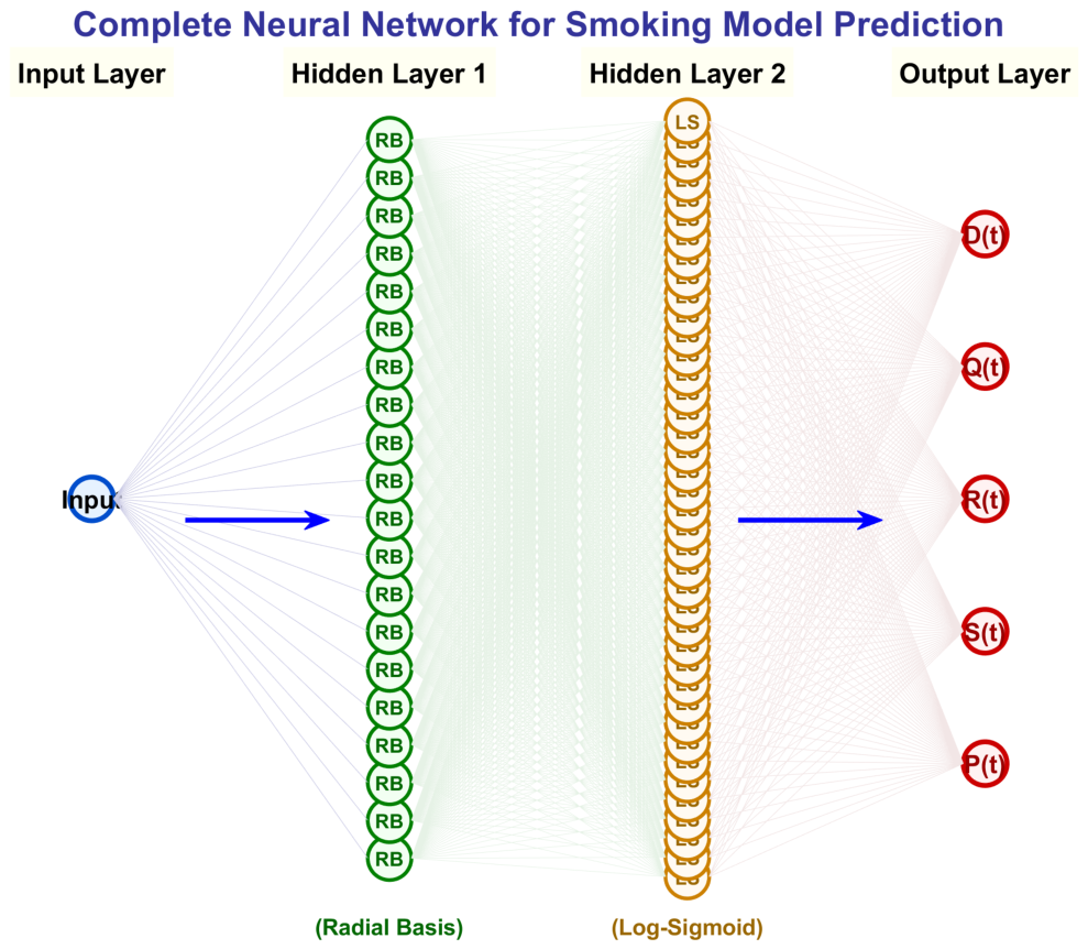
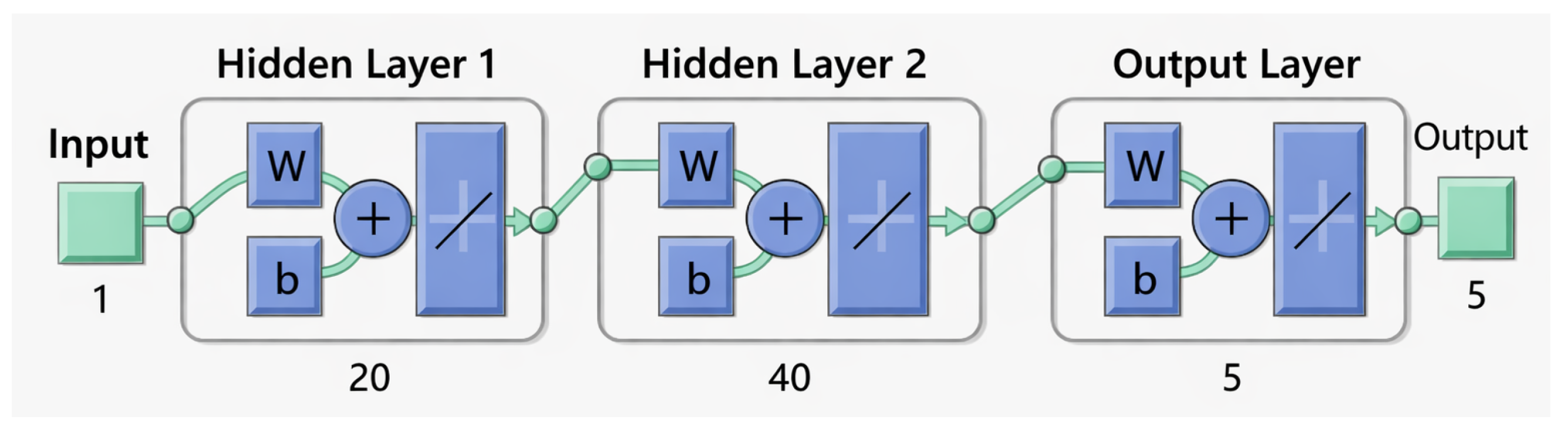
The DNN procedure is shown in Figure 1. The input in a single layer is first traversed by 20 neurons using the RBAF, and the output layer is then built using 40 neurons with the LSAF.

DNNs offer robust and adaptable frameworks when used to solve dynamical systems, especially for highly nonlinear and time-dependent models like the smoking model formulation. Without requiring precise analytical representations, DNNs can approximate arbitrarily complex nonlinear functions. By learning from reference data computed by Runge–Kutta, the DNN-LMB model in this study offers an effective means of characterizing the intricate dynamics of the population classes inside the smoking cessation framework. The NN significance in modeling epidemiological and public health systems is defined by its ability to generalize for a range of ICs and adapt to different test scenarios. Because it lowers computation expenses in the event of the subsequent process simulations, the DNN technique is a helpful tool for predicting and evaluating smoking behavior patterns in public health contexts.

We provide a new DNN strategy that uses the RBAF and LSAF in 20–40 neurons at midway layers to reach the numerical solution of the proposed model. The number of epoch options is set at 1200. Using the LMB optimization structure, the improved training performance and convergence characteristics of the proposed NN are demonstrated below. In order to minimize the MSE objective function, the LMB method modifies the network weights and biases iteratively. It is appropriate for small-to-medium-sized datasets like those in our work because it combines the stability of gradient descent with the speed of Gauss–Newton. The final phase, shown in Figure 2, applies the RBAF in the first hidden layer and the LSAF in the second hidden layer. The DNN with two hidden layers uses the parameters listed in

Table 1. An explanation of the smoking model’s factors and their numerical values.

Symbol	Description	Value
$\mathrm{\Lambda }$	Recruitment rate of potential smokers into the population	0.2
${\beta }_1$	Transmission rate from potential smokers to active smokers	$[0.01,0.9]$
${\beta }_2$	Transition rate from potential to quitter smokers (direct quitting)	$[0.005,0.03]$
$\alpha$	Smoking cessation rate (active smokers quitting)	$[0.1,0.3]$
$ϵ$	Fraction of quitters who become recovered/resistant	$[0.02,0.5]$
$\mu$	Natural death rate (unrelated to smoking)	$[0.001,0.2]$
$\varphi$	Rate of potential smokers transitioning directly to quitters	$[0.03,0.22]$
$\pi$	Fraction of recovered smokers who relapse to potential smokers	$[0.01,0.6]$
$\theta$	Relapse rate of recovered smokers	$[0.04,0.05]$
$\rho$	Rate of active smokers transitioning to recovered status	$[0.01,0.15]$
$\gamma$	Smoking-induced mortality rate	$[0.015,0.27]$

to eliminate the smoking model’s nonlinearity.

5. Discussion and Results

This section’s main goal is to provide the smoking model’s mathematical solution. Results are shown for three distinct scenarios using the DNN approach. The correlation coefficient (R) is a statistical metric used in regression analysis to assess how well the expected and actual data fit together. The fit is reliable and trustworthy since R for our model is equal to 1 or (≈1). We observe that the near-perfect regression ($R^2=1$) is predicted when training on deterministic RK4-generated reference data and is mainly used to confirm that the DNN framework is implemented correctly rather than to show that it is superior to the numerical solution. Furthermore, since the network has not been externally validated on noisy data or parameter distributions outside the training range, we acknowledge that high $R^2\approx 1$ obtained on RK4-generated datasets primarily confirm correct implementation and accurate memorization of the training trajectories rather than demonstrating genuine predictive superiority. Instead of directly solving the governing differential equations, the DNN learns to approximate the RK4-generated solution trajectories of the ODE system. This method can be used for quick surrogate prediction once trained, but it is constrained by the need for retraining when extrapolating beyond the training parameter range and the inability to independently identify the underlying differential structure. Another statistical method for evaluating the accuracy and effectiveness of regression models is the MSE, which calculates the average squared difference between expected and actual values. Error histograms were used to analyze the distribution of errors between predicted and exact values. They help in understanding a prediction model’s characteristics and performance. A range or interval of error values is represented by each bin in an error histogram, and the height of each bin indicates how frequently or how many datasets fall inside that range of errors. The MSE can be used to determine the mean squared variation between the approximated $\widehat{y_i}$ and the original $y_i$. It offers the figure that shows the network’s estimated accuracy.

$$\mathrm{MSE}={\displaystyle \frac{1}{n}}{\displaystyle \sum _{i=1}^m}{(y_i-\widehat{y_i})}^2$$

The symbol m indicates the total quantity of data points inside the set of data. The graph’s horizontal line represents a model which can consistently carry out the same. If the line that is horizontal has the lowest MSE, the model forecasts each event in the entire dataset with accuracy. In contrast, the lines are connected by a vertical line for the several models that are assessed in an MSE plot. The model that has the highest quantity of the lowest MSE values is shown by the vertical line that performs better than the others. 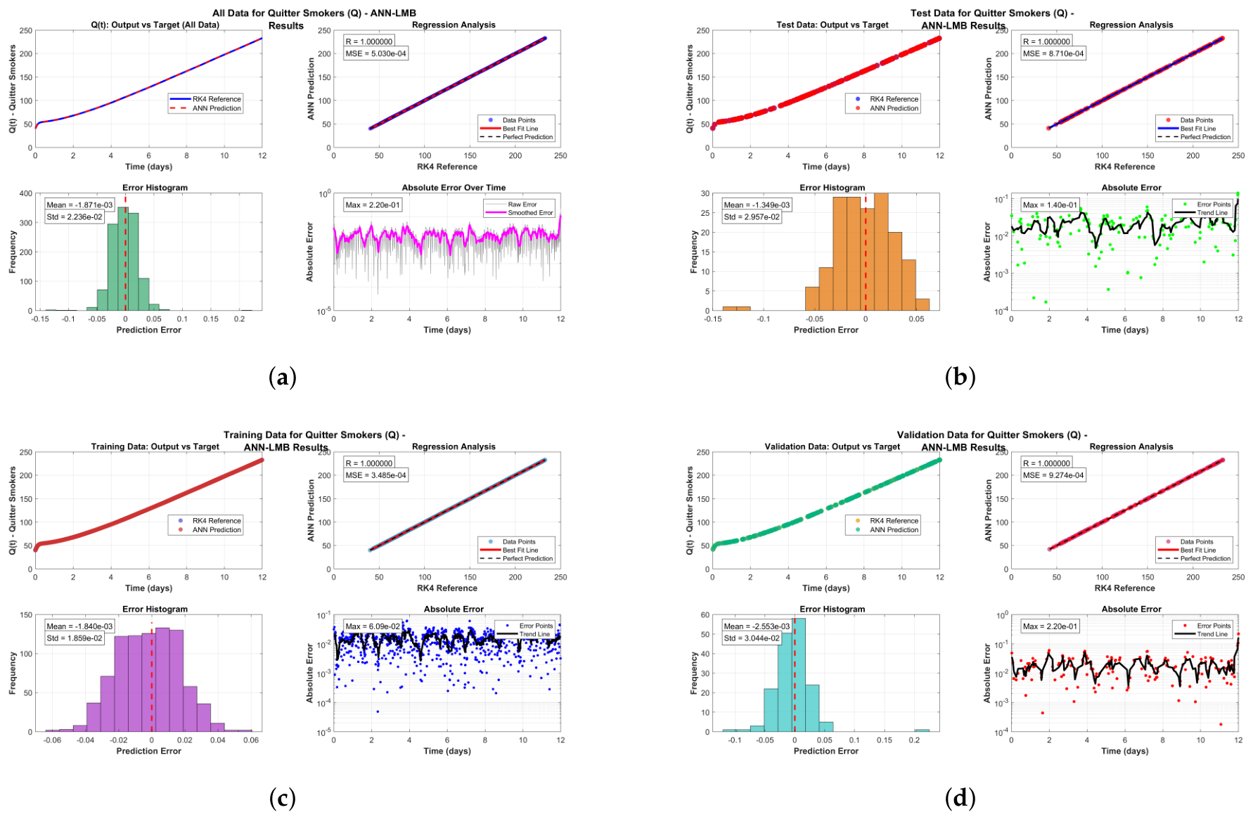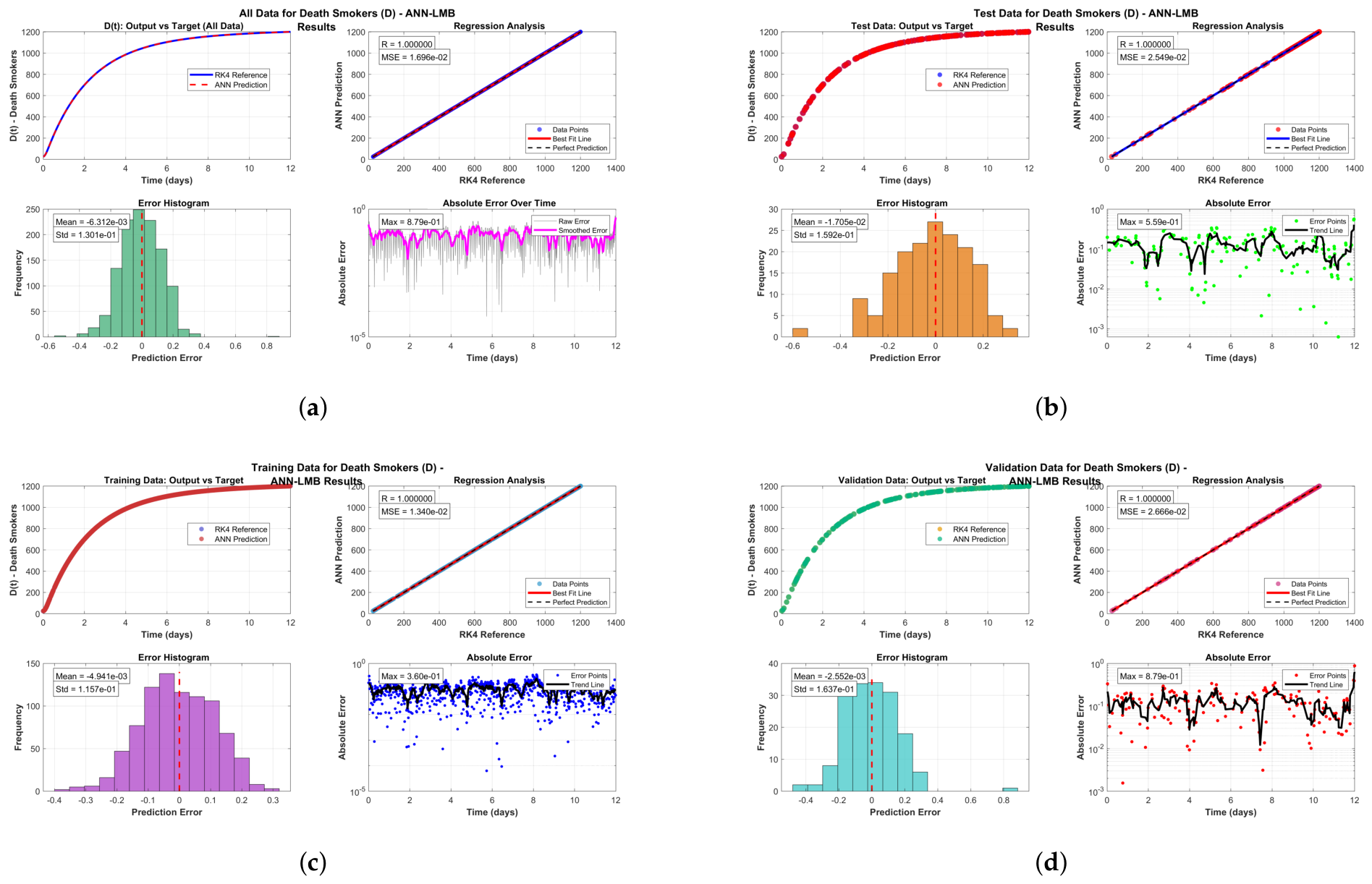Figure 3 presents the trained NN predictions for all five compartments, namely $P\left(t\right)$, $S\left(t\right)$, $R\left(t\right)$, $Q\left(t\right)$, and $D\left(t\right)$, obtained using the proposed DNN-LMB architecture (

Table 2. Algorithmic representation for DNN-LMB.

DNN-LMB Building: The reference dataset is generated using MATLAB’s fourth-order Runge–Kutta (RK4) method. Selection of Datasets: The collected data are compiled in vector or matrix form for each dataset. Setup: Select the NN, and split the data into training, test, and validation sets: Two hidden layers: 20 RBAF neurons (Layer 1) and 40 LSAF neurons (Layer 2); Using up to 70% as training data; Using up to 15% as test data; Using up to 15% as validation data. Construction of Algorithms: To create a transfer function for each input, variables are multiplied by various weights and modified using biases. Three subsets of the specified dataset are used: 15% for validation, 70% for training, and 15% for testing. Training with the entire dataset may lead to overfitting, as there is no independent set for validation and testing. Overfitting occurs when the model performs poorly on unseen data because it has memorized the training data. It becomes very difficult to evaluate the model without a separate test set. A small dataset can limit the model’s generalizability, increase the risk of overfitting, produce unreliable performance estimates, and fail to accurately represent the population. If too many data are removed, the model performs poorly and generates ambiguous predictions. If a model’s dataset is sufficiently large, it can be effectively trained and assessed. Stopping Conditions: This procedure continues until the following requirements are met: The maximum value of Mu and the maximum number of training iterations. Performance reaches a minimal value. Results are retained only while the gradient remains below the minimum gradient threshold; otherwise, the network undergoes retraining. Model Retraining: The outputs that arise from changing the network’s settings are maintained. Results Storage: At the final stage, the DNN-LMB results are stored as graphs.

). The figure illustrates the network’s ability to accurately capture the nonlinear dynamics of the smoking model across all population compartments.

5.1. Hyperparameter Selection Justification

Empirical investigation led to the selection of 20 neurons in the first hidden layer (RBAF), 40 neurons in the second hidden layer (LSAF), and 1200 training epochs. While bigger configurations (e.g., 30 RBAF + 60 LSAF) increased computational time without significantly improving accuracy (ΔMSE $<{10}^{-6}$), preliminary attempts with fewer neurons (e.g., 10 RBAF + 20 LSAF) produced higher MSE values above ${10}^{-2}$ for all compartments. Because validation error consistently converged before 200 epochs in all test cases, the epoch limit of 1200 was chosen, with the remaining epochs acting as a safety margin.

Although it is outside the purview of this methodological validation, a comprehensive ablation investigation will be undertaken in subsequent research. We note that this methodological validation does not include explicit numerical comparisons with other approaches like PINNs, Neural ODEs, and traditional ANNs; such benchmarking is intended for future study to better illustrate the relative advantages of the proposed framework.

The proposed DNN approach’s functioning is verified using conventional statistical metrics. Presenting the prediction error on the scale of predicted values, the Root Mean Square Error (RMSE), and the square root of MSE provides a straightforward grasp of the forecast variation. These evaluations metrics were computed for each of the five modules of the smoking model for every data subset used for training, testing, and validation. The numerical solutions for each situation are examined below.

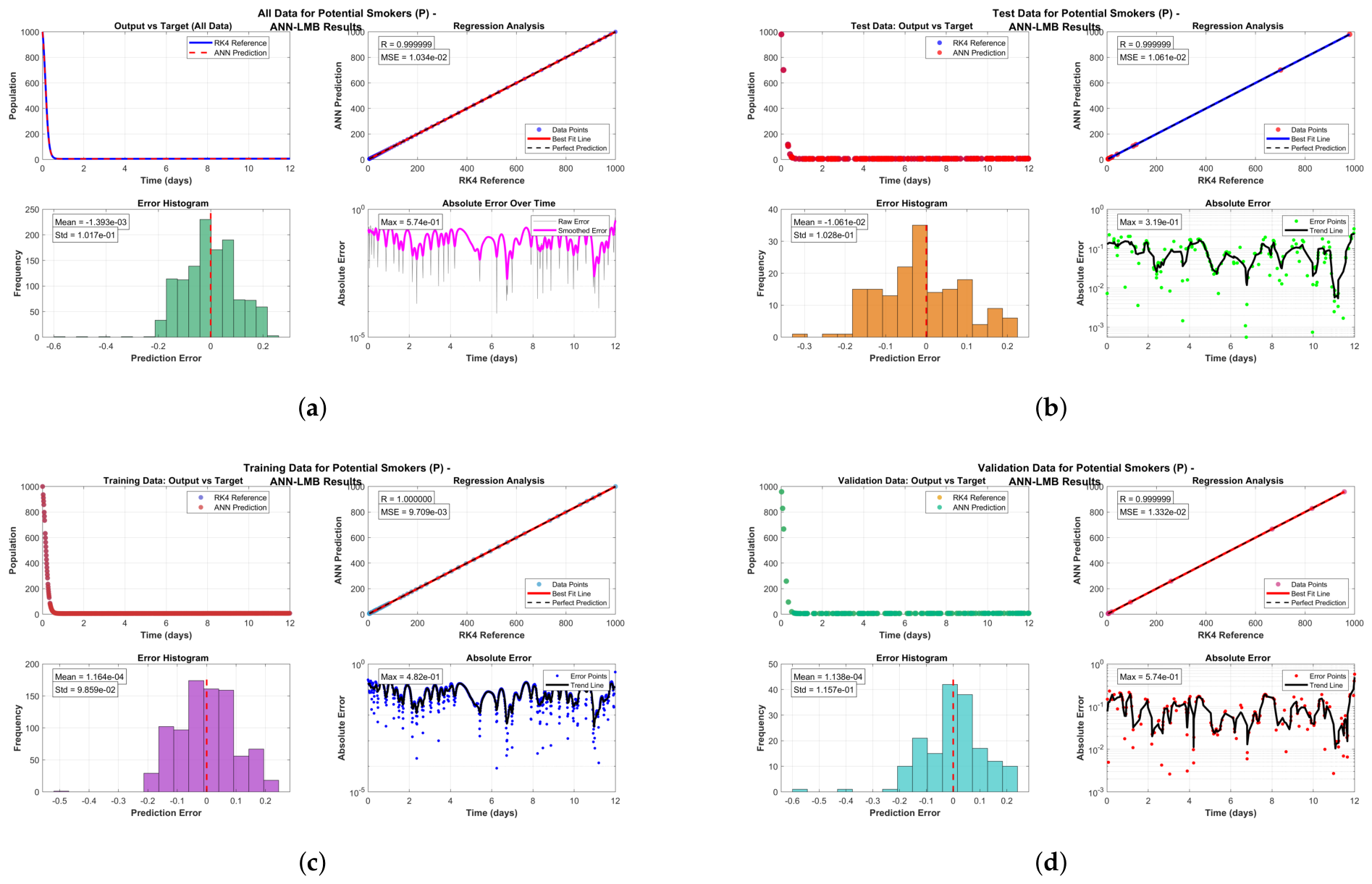
5.2. Test Problem 1

The dynamic smoking model is examined. The parameter values are taken from the available literature. $\alpha =0.1$, ${\beta }_1=0.01$, ${\beta }_2=0.005$, $\gamma =0.02$, $\rho =0.01$, $\varphi =0.03$, $\theta =0.04$, $ϵ=0.5$, $\pi =0.6$, and $\mu =0.001$. The ICs are $S\left(0\right)=200$, $P\left(0\right)=1000$, $Q\left(0\right)=30$, $R\left(0\right)=50$, and $D\left(0\right)=10$. The numerical solution for this test problem is shown in Figure 4, which presents the MSE performance for potential smokers (P).

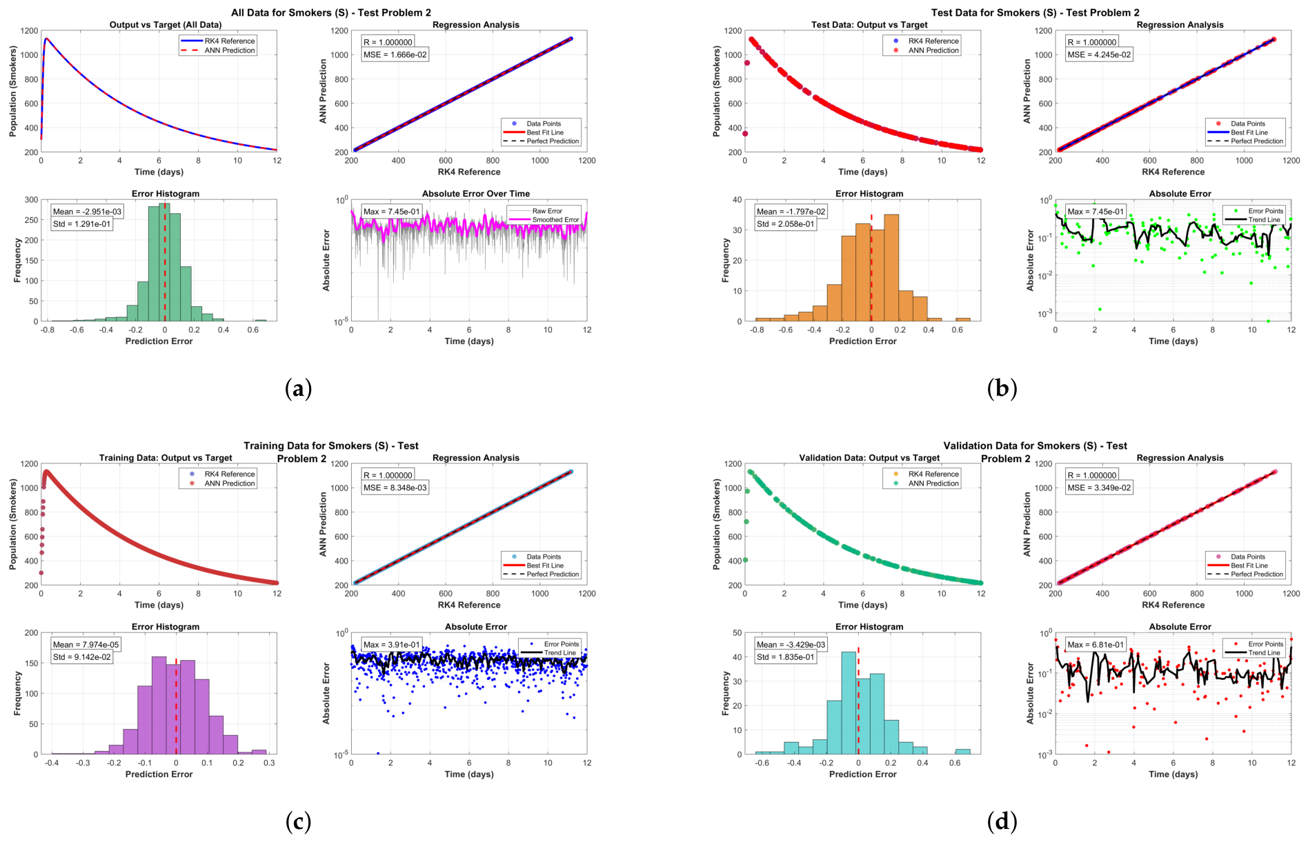
5.3. Test Problem 2

The smoking dynamics model is considered. The parameter values are sourced from the literature. The revised values of $\alpha$ and ${\beta }_1$—that is, $\alpha =0.3$ and ${\beta }_1=0.02$—are considered, and the remaining values are the same as those stated in Test Problem 1. $S\left(0\right)=300$, $P\left(0\right)=800$, $Q\left(0\right)=20$, $R\left(0\right)=100$, and $D\left(0\right)=5$ are the ICs. The MSE performance for active smokers (S) corresponding to this test problem is provided in Figure 5.

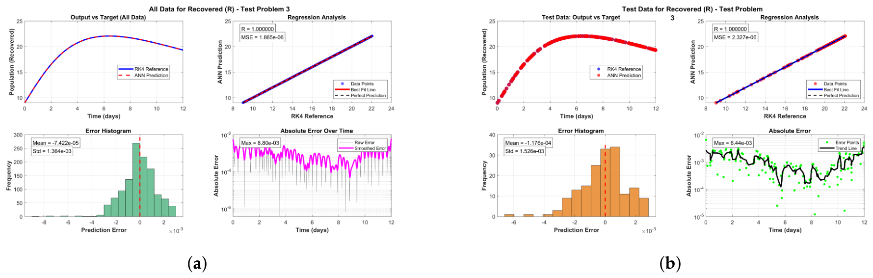
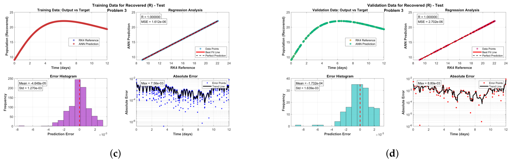
5.4. Test Problem 3

The provided dynamics model is taken into consideration. The literature is the source of the parameter values. Following the four-parameter variation pattern in comparative research, the updated values of four parameters, $\alpha =0.16$, $\gamma =0.23$, $\rho =0.08$, and $\varphi =0.19$, are considered. The remaining parameters are identical to those listed in Test Problem 1. $S\left(0\right)=28$, $P\left(0\right)=55$, $Q\left(0\right)=4$, $R\left(0\right)=9$, and $D\left(0\right)=2$ are the ICs. The MSE-based numerical results for this test problem are visualized in Figure 6, specifically for the recovered smoker (R) category.

5.5. Test Problem 4

We examine the smoking dynamics model that is provided. The literature is the source of the parameter values. According to the four-parameter variation pattern in the comparative study, the updated values of four parameters, $\alpha =0.25$, $\gamma =0.12$, $\rho =0.15$, and $\varphi =0.08$, are taken into consideration. The remaining parameters are same as those listed in Test Problem 1. $S\left(0\right)=350$, $P\left(0\right)=1200$, $Q\left(0\right)=45$, $R\left(0\right)=80$, and $D\left(0\right)=15$ are the ICs. Figure 7 provides the numerical solution for this test problem, illustrating the MSE performance for quitter smokers (Q) across all datasets.

5.6. Test Problem 5

We consider the given smoking dynamics model. The parameter values come from the literature. The revised values of four parameters, $\alpha =0.18$, $\gamma =0.27$, $\rho =0.12$, and $\varphi =0.22$, are taken into consideration in accordance with the pattern of four-parameter variation in comparative research. The remaining parameters are the same as those mentioned in Test Problem 1. The ICs are $S\left(0\right)=400$, $P\left(0\right)=1500$, $Q\left(0\right)=60$, $R\left(0\right)=100$, and $D\left(0\right)=25$. This test problem’s solution is depicted in Figure 8, which corresponds to the MSE performance of death smokers (D).

Table 3. Complete performance metrics (MSE, RMSE, coefficient of determination, histogram mean error, and standard deviation) for all compartments across training, test, validation, and all-data sets for Test Problems 1–5.

Comp.	Dataset	MSE	RMSE	${\mathit{R}}^2$	Hist. Mean	Hist. SD	Max Abs Error
P	All	$1.034\times {10}^{-2}$	$1.017\times {10}^{-1}$	$0.999998$	$-1.393\times {10}^{-3}$	$1.017\times {10}^{-1}$	$5.74\times {10}^{-1}$
	Test	$1.061\times {10}^{-2}$	$1.030\times {10}^{-1}$	$0.999998$	$-1.061\times {10}^{-2}$	$1.028\times {10}^{-1}$	$3.19\times {10}^{-1}$
	Training	$9.709\times {10}^{-3}$	$9.854\times {10}^{-2}$	$1.000000$	$1.164\times {10}^{-4}$	$9.859\times {10}^{-2}$	$4.82\times {10}^{-1}$
	Validation	$1.332\times {10}^{-2}$	$1.154\times {10}^{-1}$	$0.999998$	$1.138\times {10}^{-4}$	$1.157\times {10}^{-1}$	$5.74\times {10}^{-1}$
S	All	$1.666\times {10}^{-2}$	$1.291\times {10}^{-1}$	$1.000000$	$-2.951\times {10}^{-3}$	$1.291\times {10}^{-1}$	$7.45\times {10}^{-1}$
	Test	$4.245\times {10}^{-2}$	$2.060\times {10}^{-1}$	$1.000000$	$-1.797\times {10}^{-2}$	$2.058\times {10}^{-1}$	$7.45\times {10}^{-1}$
	Training	$8.348\times {10}^{-3}$	$9.137\times {10}^{-2}$	$1.000000$	$7.974\times {10}^{-5}$	$9.142\times {10}^{-2}$	$3.91\times {10}^{-1}$
	Validation	$3.349\times {10}^{-2}$	$1.830\times {10}^{-1}$	$1.000000$	$-3.429\times {10}^{-3}$	$1.835\times {10}^{-1}$	$6.81\times {10}^{-1}$
R	All	$1.865\times {10}^{-6}$	$1.364\times {10}^{-3}$	$1.000000$	$-7.422\times {10}^{-5}$	$1.364\times {10}^{-3}$	$8.80\times {10}^{-3}$
	Test	$2.327\times {10}^{-6}$	$1.525\times {10}^{-3}$	$1.000000$	$-1.176\times {10}^{-4}$	$1.526\times {10}^{-3}$	$6.44\times {10}^{-3}$
	Training	$1.612\times {10}^{-6}$	$1.270\times {10}^{-3}$	$1.000000$	$-4.648\times {10}^{-5}$	$1.270\times {10}^{-3}$	$7.56\times {10}^{-3}$
	Validation	$2.702\times {10}^{-6}$	$1.639\times {10}^{-3}$	$1.000000$	$-1.732\times {10}^{-4}$	$1.639\times {10}^{-3}$	$8.80\times {10}^{-3}$
Q	All	$5.030\times {10}^{-4}$	$2.236\times {10}^{-2}$	$1.000000$	$-1.871\times {10}^{-3}$	$2.236\times {10}^{-2}$	$2.20\times {10}^{-1}$
	Test	$8.710\times {10}^{-4}$	$2.951\times {10}^{-2}$	$1.000000$	$-1.349\times {10}^{-3}$	$2.957\times {10}^{-2}$	$1.40\times {10}^{-1}$
	Training	$3.485\times {10}^{-4}$	$1.867\times {10}^{-2}$	$1.000000$	$-1.840\times {10}^{-3}$	$1.859\times {10}^{-2}$	$6.09\times {10}^{-2}$
	Validation	$9.274\times {10}^{-4}$	$3.044\times {10}^{-2}$	$1.000000$	$-2.553\times {10}^{-3}$	$3.044\times {10}^{-2}$	$2.20\times {10}^{-1}$
D	All	$1.696\times {10}^{-2}$	$1.302\times {10}^{-1}$	$1.000000$	$-6.312\times {10}^{-3}$	$1.301\times {10}^{-1}$	$8.79\times {10}^{-1}$
	Test	$2.549\times {10}^{-2}$	$1.597\times {10}^{-1}$	$1.000000$	$-1.705\times {10}^{-2}$	$1.592\times {10}^{-1}$	$5.59\times {10}^{-1}$
	Training	$1.340\times {10}^{-2}$	$1.158\times {10}^{-1}$	$1.000000$	$-4.941\times {10}^{-3}$	$1.157\times {10}^{-1}$	$3.60\times {10}^{-1}$
	Validation	$2.666\times {10}^{-2}$	$1.633\times {10}^{-1}$	$1.000000$	$-2.552\times {10}^{-3}$	$1.637\times {10}^{-1}$	$8.79\times {10}^{-1}$

summarizes the full numerical results for each of the five test problems and five compartments (P, S, R, Q, and D). Near-perfect regression ($R^2=1$ or ≈1) is achieved by the DNN-LMB framework on all datasets (training, test, validation, and all data). In Test Problem 3, the recovered smoker (R) compartment has the lowest MSE ($1.865\times {10}^{-6}$) and RMSE ($1.364\times {10}^{-3}$). Error histograms show that all compartments’ mean errors are constantly close to zero with modest standard deviations, indicating the proposed method’s exceptional accuracy and capacity for generalization. This complete table has been created by condensing the repetitious textual descriptions.

5.7. Epidemiological Interpretation of Smoking Dynamics

Several epidemiologically relevant trends are shown by the DNN solutions for each of the five test problems. Because recruitment ($\mathrm{\Lambda }$) is countered by transmission to active smoking (${\beta }_{1}PS$) and direct quitting (${\beta }_{2}P$ and $\varphi P$), the potential smoker compartment $P\left(t\right)$ steadily declines over time. The balance between initiation from potential smokers and removal via quitting ($\alpha$), recovery ($\rho$), and smoking-induced mortality ($\gamma$) is reflected in the active smoker compartment $S\left(t\right)$, which shows a peak followed by a slow drop. Although relapse ($\pi \theta R$) back into possible smoking is still a persistent challenge, the recovered compartment $R\left(t\right)$ exhibits steady expansion in most circumstances, indicating effective long-term quitting. Notably, the death compartment $D\left(t\right)$ continuously increases, highlighting smoking’s long-term mortality impact, while the quitter compartment $Q\left(t\right)$ stays relatively small compared with $R\left(t\right)$ because quitters either stay in $Q\left(t\right)$ or go elsewhere. These interpretations show that the DNN framework maintains the basic epidemiological logic of smoking transmission rather than just fitting numerical curves.

5.8. Public Health Implications

The proposed DNN architecture immediately addresses public health problems by providing quick, real-time forecasts of smoking dynamics under various intervention scenarios, even though this study’s main contribution is methodological. Every time a parameter changes (e.g., increase in smoking cessation rate $\alpha$ or reduction in relapse rate $\theta$), traditional RK4 approaches necessitate a full re-solving of the ODE system. On the other hand, the trained DNN offers instantaneous predictions for new parameter sets and initial conditions following a single offline training run. When assessing questions like “What would be the impact on active smokers (S) and smoking-related deaths (D) over 10 years if relapse rates ($\theta$) were reduced by 30%?” or “How many additional quitters (Q) would result from a media campaign that increases $\varphi$ (direct quitting from potential smokers) by 50%?” The DNN architecture may produce instantaneous answers to such queries without requiring any numerical ODE solver at the time of prediction, enabling evidence-based decision making for tobacco taxation, public awareness campaigns, and smoking cessation programs. In order to calibrate the model for particular demographics, future study will use actual clinical and census data.

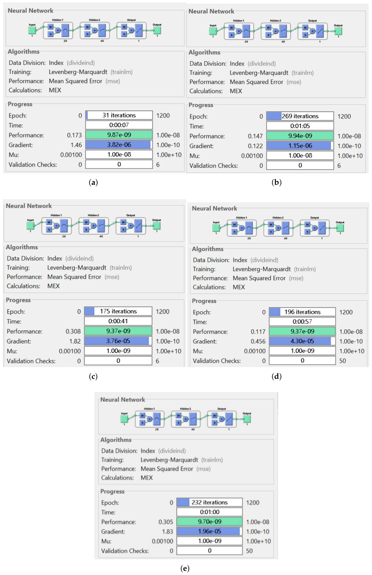
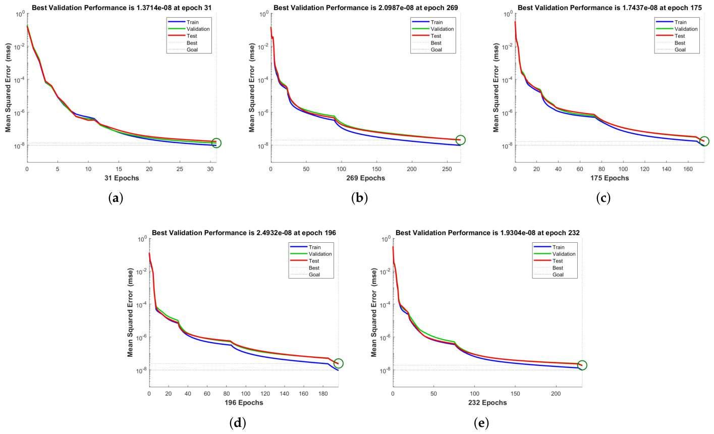
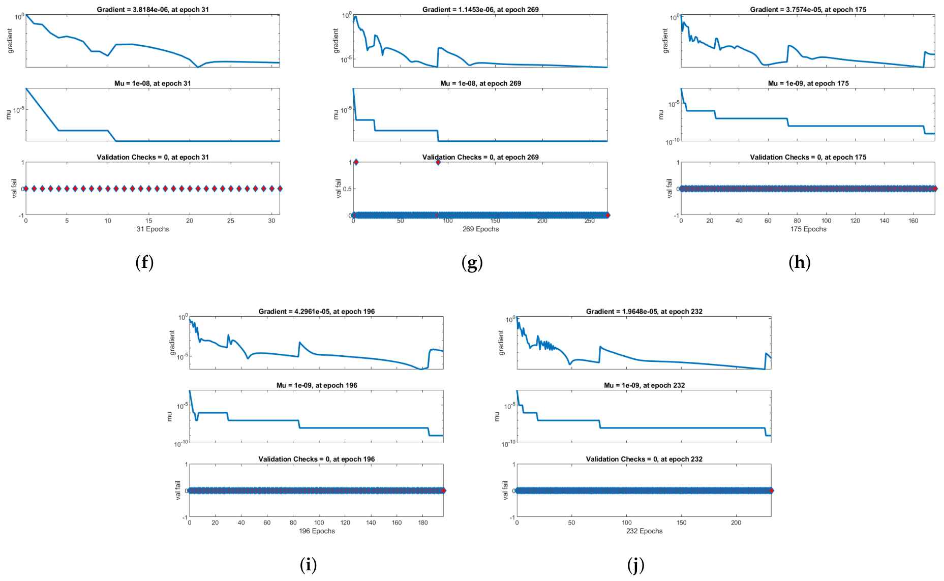
The proposed deterministic method for solving the nonlinear smoking dynamics model is used to illustrate the gradient measures and optimal training performance in Figure 9. Large-scale deep learning frameworks, intricate optimization, and massive datasets are all incorporated into the best training form based on the MSE. To examine the enhanced iteration performance throughout the entire training set using learning techniques, the number of epochs was chosen to be 1200 while maintaining the twin-hidden-layer construction.

MSE performance for each of the five compartments (P, S, R, Q, and D) is shown in Figure 9. The MSE values are found to be $1.3714\times {10}^{-8}$ at 31 epochs, $2.0987\times {10}^{-8}$ at 269 epochs, $1.7437\times {10}^{-8}$ at 175 epochs, $2.4932\times {10}^{-8}$ at 196 epochs, and $1.9304\times {10}^{-8}$ at 232 epochs. The gradient, Mu, and validity check-based illustrations are displayed in the second row of Figure 9 for the P, S, R, Q, and D compartments, respectively, provided as the function based on the optimization process. The gradient values for the P, S, R, Q, and D compartments are found to be $3.8184\times {10}^{-6}$, $1.1453\times {10}^{-6}$, $3.7574\times {10}^{-5}$, $4.2961\times {10}^{-5}$, and $1.9648\times {10}^{-5}$, achieved at epochs 31, 269, 175, 196, and 232, respectively. By improving a function, which is typically carried out in optimization procedures to attain the minimum and maximum function values, these plots indicate the direction of the steepest descent.

The step sizes used for the parameter of the system during the phase of learning are $1\times {10}^{-8}$ for the P and S compartments and $1\times {10}^{-9}$ for the R, Q, and D compartments. The excellent generalization capability of the proposed DNN architecture is confirmed by the zero validation checks for all compartments, which show that the validation error never increased during the training process. Authentication checks provide a foundation for justifying the network’s characteristics.

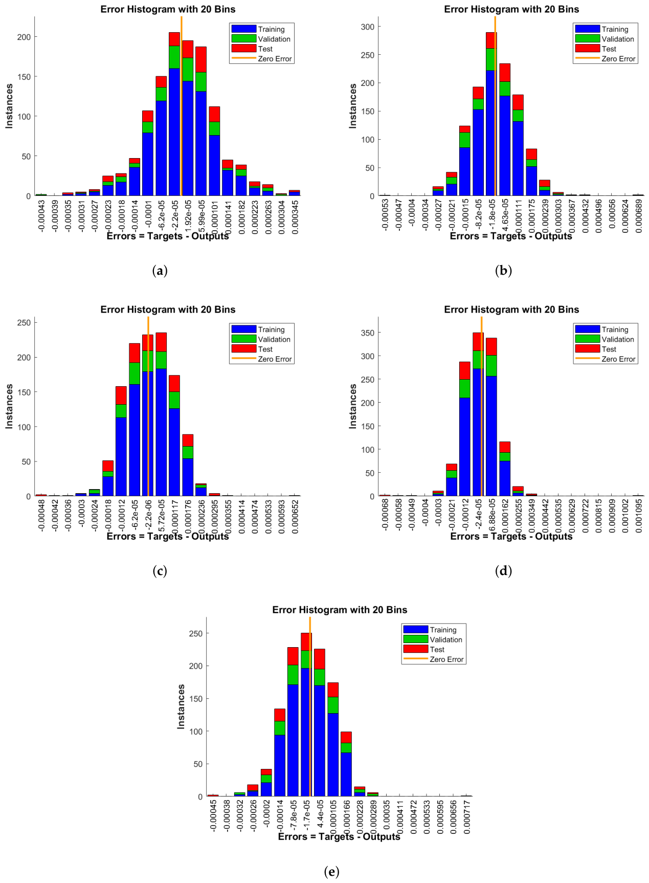
By combining the DNN with the RBAF and the LSAF, the nonlinear smoking dynamics model is presented using the resulting values of the error histogram (EH) in Figure 10. The EH is used to assess the system’s accuracy and evaluate the predicted outcomes. Error distributions that display the frequency of instances across various error bins are given to the EH performance for each of the five compartments (P, S, R, Q, and D). The concentration of samples near the zero-error line demonstrates the accuracy of the proposed approach. The accuracy and dependability of the DNN architecture used to solve the smoking dynamics model are confirmed by the error values for each compartment remaining within insignificant ranges.

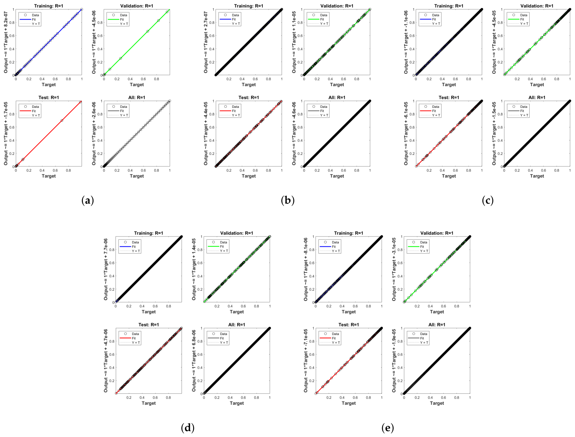
The regression analysis for each of the smoking dynamics model’s five compartments (P, S, R, Q, and D) using the proposed DNN architecture is shown in Figure 11. For each variation, regression is computed about 1, demonstrating the ideal modeling form. The line that fits the best, which illustrates the relationships between the variables, is found using regression data. The regression equations for the P compartment are as follows: (Validation) Output = 1 × Target + 4.5 $\times {10}^{-6}$, (Training) Output = 1 × Target + 8.2 $\times {10}^{-7}$, (All Data) Output = 1 × Target − 2.6 $\times {10}^{-6}$, and (Test) Output = 1 × Target + 1.7 $\times {10}^{-5}$. RK4 reference solutions and the DNN predictions have an exact linear relationship, as demonstrated by the perfect regression values of R = 1 in all other compartments (S, R, Q, and D). The exceptional accuracy and dependability of the proposed approach in resolving the nonlinear smoking dynamics model are validated by this exact correlation.

The various performance metrics for each of the five compartments of the smoking dynamics model utilizing the proposed DNN architecture are given in

Table 4. Different performance results of the nonlinear smoking dynamics model using the DNN.

Compartment	MSE			Gradient	Performance	Epochs
	Training	Validation	Test
P	$9.709\times {10}^{-3}$	$1.332\times {10}^{-2}$	$1.061\times {10}^{-2}$	$3.8184\times {10}^{-6}$	$1.3714\times {10}^{-8}$	31
S	$8.348\times {10}^{-3}$	$3.349\times {10}^{-2}$	$4.245\times {10}^{-2}$	$1.1453\times {10}^{-6}$	$2.0987\times {10}^{-8}$	269
R	$1.612\times {10}^{-6}$	$2.702\times {10}^{-6}$	$2.327\times {10}^{-6}$	$3.7574\times {10}^{-5}$	$1.7437\times {10}^{-8}$	175
Q	$3.485\times {10}^{-4}$	$9.274\times {10}^{-4}$	$8.710\times {10}^{-4}$	$4.2961\times {10}^{-5}$	$2.4932\times {10}^{-8}$	196
D	$1.340\times {10}^{-2}$	$2.666\times {10}^{-2}$	$2.549\times {10}^{-2}$	$1.9648\times {10}^{-5}$	$1.9304\times {10}^{-8}$	232

. The test, validation, and training subsets’ MSE values are presented, together with the gradient, optimal performance, epochs, and computational time. The remarkable accuracy and effective convergence of the developed methods are confirmed by the minimal MSE values and gradient around zero.

6. Conclusions

The five-compartment smoking model (potential smokers P, active smokers S, quitters Q, recovered R, and deaths D) was successfully implemented using a unique dual-hidden-layer DNN architecture that included 20 RBAF neurons and 40 LSAF neurons and was optimized using the Levenberg–Marquardt method. The main findings are as follows: (1) the DNN achieved remarkable accuracy with MSE values of $1.034\times {10}^{-2}$ (P), $1.666\times {10}^{-2}$ (S), $1.865\times {10}^{-6}$ (R), $5.030\times {10}^{-4}$ (Q), and $1.696\times {10}^{-2}$ (D) for all datasets; (2) $R^2$ = 1 or nearly 1 for all compartments; and (3) the model effectively captured the smoking dynamics of public health significance. This study’s primary contribution is the effective application and validation of a dual-hidden-layer DNN framework for very accurate prediction of the smoking model’s dynamics.

The trained DNN offers instantaneous predictions, in contrast to RK4, which necessitates explicit equation re-solving for every parameter change. This makes it useful for public health officials assessing intervention plans like smoking bans, treatment programs, or media campaigns. It should be mentioned that the current study employs benchmark parameter sets and initial conditions taken from the literature to validate the proposed DNN framework. The goal of the proposed DNN framework is to create a machine learning-based foundation that can be expanded to data-driven tasks like parameter estimation, uncertainty quantification, surrogate modeling, and real-time prediction, where traditional numerical solvers may be less flexible, even though the RK4 method is still computationally more effective for the forward simulation of low-dimensional ODE systems.

The research gap in current smoking dynamics models—conventional numerical approaches are computationally stiff and do not integrate with machine learning for real-time public health applications—was addressed by this work. A logical next step would be to extend the proposed DNN framework to solve inverse problems, such as estimating unknown or time-varying parameters (e.g., cessation rate $\alpha$ or relapse rate $\theta$) from real-world noisy smoking prevalence data. This would take advantage of the fundamental utility of machine learning for tracking public health. Future research will take into account the use of real-world clinical, epidemiological, and census-based smoking datasets for model validation and calibration. The proposed dual-layer NN architecture can be extended in future research to address a variety of intricate epidemiological models, public health dynamics, and other mathematical biology nonlinear systems [25].