


Abstract
In this work, we propose an inertial proximal splitting algorithm for the split variational inclusion problem in real Hilbert space, in which a new stepsize rule is provided for avoiding the case that the original stepsize equals to zero, It also helps enlarge the value range of the stepsize parameter. A weak and strong convergence theorem is established under mild conditions. Additionally, our obtained result is extended to split feasibility problems and split minimization problems. Finally, some numerical experiments are conducted to illustrate and compare.
Keywords:
split variational inclusion problem; splitting algorithm; inertial technique; strong convergence MSC:
47J20; 65K05; 65K10; 47J25
1. Introduction
Let X be a real Hilbert space with induced norm and inner product . Let be a maximally monotone multi-valued operator. It is known that the classical split variational inclusion problem [1] (SVIP) is stated as
where and are both real Hilbert spaces, and are both monotone operators, and is a bounded linear operator. The solution set of SVIP is denoted by
The SVIP has many applications such as split variational inequalities, image restoration, Generative Adversarial Networks (GANs) and so on (see [2,3,4,5,6,7,8]). Some problems are usually used as a model in image recovery [9,10] and signal recovery [8], in which the signal recovery can be transformed to its special case; that is, the split feasibility problem (SFP) [11] is expressed as
in which C and Q are nonempty, closed, and convex subsets of and , respectively.
1.1. Related Algorithms
Due to its wide applications, many existing methods are used to deal with SVIP and its nonlinear programming problems (see the concrete introductions of [2,3,4,5,6,7,12,13,14] for reference). Additionally, a well-known approach to deal with the SVIP is Byrne’s algorithm [15], whose frame is the following:
where is defined in Section 2, is a parameter, is a fixed stepsize, and is a adjoint operator of A. With the help of the fixed stepsize , the weak convergence of the above algorithm was obtained. However, Byrne’s algorithm is the first to calculate the norm in each iteration, which is somewhat difficult, if A is a dense matrix in practice. Regarding this consideration, this is usually avoided by an Armijo-linear search rule. Based on the rule, there are many proximal splitting algorithms emerging for solving the SVIP (detailed information can be found in [2,4,5,6,13,14] for reference). Since the Armijo-linear search rule generally makes the algorithm produce the inner iterations, the algorithm efficiency is affected. To overcome this, Lopéz [16] proposed a self-adaptive stepsize strategy below:
with and and and can be expressed as the corresponding projections onto Q. For more details on this self-adaptive stepsize strategy, see [17,18,19,20]. Follow by this, the inertial extrapolation technique has received much more attention, and which is popularly used to increase the convergence (see, for instance, [21,22,23,24,25,26,27,28]). Among them, Nesterov [28] used the inertial technique to speed up the heavy ball method [18] in the following.
where and . The term is the so-called inertial term. Recently, Thong [29] proposed a self-adaptive inertial subgradient extragradient method for solving non-monotone variational inequalities, and he obtained its weak convergence in real Hilbert space. Its iterative scheme is of the following form:
where the stepsize is updated by
where , is a sequence of nonnegative real numbers that satisfies , , , , and , is a uniformly continuous mapping on X. Based on Lopéz’s stepsize thought [16], Cholamjiak et al. [30] suggested a linearized splitting algorithm for solving the SVIP, with the scheme
where the stepsize is given by
Here, both and its gradient are defined in Section 3. and and satisfies . Under these conditions, it is shown that the sequence created by the algorithm converges weakly to a point in Very recently, Xu et al. [31] introduced an inertial viscosity-type projection and contraction algorithm for addressing quasimonotone variational inequalities. The iterative form is described as follows:
where the stepsizes and are respectively defined as
where , , , , , for some , , and and are the inertial parameters. is a Lipschitz continuous and quasimonotone mapping, is a contraction mapping with constant and The strong convergence of the algorithm (8) is discussed in real Hilbert spaces.
1.2. Motivation and Contributions
For the existing proximal gradient methods, e.g., Byrne’s algorithm (4), the new iterative algorithms [5,32,33], and the inertial proximal algorithm [2,4,6,34,35,36], their convergence holds under assumptions on the inverse strongly monotonicity of and this condition brings a small stepsize , which may consume more computational time. On the other hand, it may produce many iterative numbers when the Armijo-linear search in [21] aims to find a proper stepsize in the iterative process. Additionally, we observe that when the stepsize in Algorithm (7). These above considerations may affect the convergent rate of our listed algorithms. However, the weak and strong convergence of Algorithm (7) with the new stepsizes has yet to be investigated.
From these factors, we need to further improve the numerical results of Algorithm (7). Our contributions in this paper are the following.
- −
- To design a new stepsize for avoiding the case that the original stepsize is equal to zero under This helps enhance the numerical efficiency of Algorithm (7).
- −
- To modify the iterative term to be a proximal point, which is suggested in [37]. This enlarges from to , respectively, which helps improve the numerical results of Algorithm (7).
- −
- To discuss a strong convergence theorem of our proposed algorithm by introducing the viscosity algorithm described in [31].
- −
- To provide a theoretical application to split minimization problems and split feasibility problems, numerical experiments are conducted to demonstrate and compare.
1.3. Organization
This work is constructed as follows. Several theory results are stated in Section 2. We firstly introduce our algorithm and discuss its weak convergence in Section 3. The strong convergence analysis is presented in Section 4. In Section 5, we present an application. Some experiments are conducted to demonstrate the advantages of all compared algorithms in Section 6. Finally, we present a conclusion and discussion, respectively.
2. Preliminaries
Definition 1
([4]). Let X be a real Hilbert space. A single-value mapping is named
(a) nonexpansive if
(b) firmly-nonexpansive if
Let be a set-value maximal monotone operator. The resolvent operator related to Y is defined by
where On the other hand, , the domain of is defined by , and the fixed point set of is denoted by ; that is,
Lemma 1.
Let , for all . Then
(a) ,
(b) .
Lemma 2
([8]). Let and be real Hilbert spaces, be a bounded linear operator with its adjoint , and . Let be a set-valued maximal monotone mapping. Define a mapping by for all . Then, the following statements hold:
(a) ;
(b) .
Lemma 3
(Demiclosedness principle [32]). Assume that is a nonexpansive mapping. Then we obtain the following:
where C is described in (3).
Lemma 4
([38,39]). Let be a set-valued maximal monotone mapping and . Then the following properties hold:
(a) is a single-valued and firmly nonexpansive mapping;
(b) and ;
(c) for all and ;
(d) is a firmly nonexpansive mapping.
(e) For , one has , and
Lemma 5
([8]). Let and be the two real Hilbert spaces, and be a bounded linear operator with its adjoint operator . Let , , and be set-valued maximal monotone mappings. For any , the following results hold:
(a) Suppose that is a solution of the SVIP. Then .
(b) If and the solution set of the SVIP is nonempty, then is a solution of the SVIP.
Lemma 6
([40]). Let be a sequence of nonnegative numbers fulfilling
where and are sequences of nonnegative numbers such that , and . Then exists.
Lemma 7
([30]). Let be a non-empty set, and be a sequence in X that fulfills the conditions below:
(a) exists for all ;
(b) every sequential weak limit sequence of is in C.
Then converges weakly to a point in C.
Lemma 8
([30]). Let and be real positive sequences such that
If and , then exists.
Lemma 9
([30]). Let and be real positive sequences such that
Then where . Additionally, if , then is bounded.
Let C be a nonempty closed and convex subset of X. Then the orthogonal projection of p onto C is defined by
Lemma 10
([19]). Let C be a nonempty closed convex subset of a real Hilbert space X and let be the metric projection from X onto C. Then the following statements hold:
(a)
(b)
(c)
Lemma 11
([41]). Suppose that is a sequence of nonnegative real numbers, such that , and let be a sequence of real numbers. Let
In addition, suppose that for any subsequence of integers fulfilling it holds that Then it is verified that
3. Weak Convergence
In this section, we propose an inertial proximal algorithm for solving Problem (1), and establish its weak convergence. First, we introduce the following assumptions for the convergence analysis before presenting our algorithmic frame.
(T1) Let the solution set of the split variational inclusion problem be nonempty, that is,
(T2) Let and be real Hilbert spaces, and let be a bounded linear operator with its adjoint Let and be set-valued maximal monotone operators.
(T3) Suppose that both and are real Hilbert spaces, and let be a bounded linear operator with its adjoint Now we define the following function
As shown in [23,42], its gradient is the following.
As described in [43], the gradient is an inverse strongly monotone operator, so it is Lipschitzian.
Now, our proposed algorithm reads as follows (Algorithm 1).
| Algorithm 1: An inertial splitting algorithm for solving the SVIP |
Step 0: Given , , Initialize , , satisfying Lemma 6. Iterative steps: Update via Step 1: Given , satisfy Step 2: Compute Step 3: Update Step 4: Update the stepsize via Step 5: Set and go to Step 1. |
Next, we illustrate that our given stepsize rule is well-defined.
Lemma 12.
Let the sequence be created by Algorithm 1. Then we attain , , where is an initial stepsize.
Proof.
Since the mapping is firmly nonexpansive, if we suppose that , we obtain
After that arrangement, we see that
which further implies that
This together with and (12), we obtain
By induction, the sequence is of a lower bound . Using (12) again, we directly arrive at . From Lemma 6 with , the limit exists and we denote by . Since , then . □
According to Lemma 12, we discuss the following weak convergence of our proposed algorithm.
Theorem 1.
Suppose that Assumptions (T1–T3) holds. Then the sequence created by Algorithm 1 converges weakly to a solution .
Proof.
Let . Then and . Therefore, we attain . By Lemma 2(a), we see that
Now, from (11) and , we have
Using (12) and (14), we see that
Since
where and . Thus, , , . Thereby, ,
By a similar analysis of (14), we directly obtain
By applying (17), we show that
This, working with (15), (16), (18) and Lemma 1(a), yields that ,
By (19), , and the inertial step (10), we further have
From Lemma 9, it yields that
where . Combining and Lemma 9, we deduce that the sequence is bounded. Thus, . Since , and by Lemma 8 and (20) again, we show that exists. From the definition of the inertial step (10), we obtain
After arrangement by substituting (22) into (19), it follows that ,
Since exists, , and by (23), one has
Since , and , we further show that
Since , it follows from (24) that
Since , and , we have
By , and , it easily obtains
Since , we have , by the definition of , we have , we further obtain
Using (26) and (27), we also see that
Combining (24) and (26), one has
This, combining with (26), (28) and (29), deduces that
Combining this with (27), it yields that
Using (25) and (27), we see that
From (27) and (31), one sees that
Let be a weak cluster point of the sequence . That is, there is a subsequence of such that . We know that A is a bounded linear operator, so we obtain . Using (32) and (33), Lemma 3 and Lemma 4(b), we show that . Using Lemma 7 again, we see that .□
4. Strong Convergence
In this section, we propose a viscosity-type inertial splitting algorithm for solving the SVIP, and we establish its strong convergence in real Hilbert space. Now, we present the following assumptions for the convergence analysis.
is a contraction mapping with constant
, , , and Our strongly convergent algorithm is summarized in the following.
Remark 1.
In Algorithm 2, the inertial parameter is selected as
Remark 2.
By Algorithm 2, it is verified that Indeed, we derive for all , which, together with , yields that
Theorem 2.
Assume that Conditions – hold. Then the sequence created by Algorithm 2 converges strongly to a point , where .
| Algorithm 2: An inertial viscosity-type splitting algorithm for solving the SVIP |
Step 0: Given , , Initialize , , satisfying Lemma 6. Iterative steps: Update via Step 1: Given , satisfy Step 2: Compute Step 3: Update Step 4: Update the stepsize via Step 5: Set and go to Step 1. |
Proof.
According to the expression (19), we directly obtain
By the definition of the inertial step , one has
According to Remark 2, there is a constant such that
Combining (38), (39) and (40), we show that
This verifies that
This result shows that the sequence is bounded. It is also shown that the sequences and are bounded. Additionally, we have
for some this, together with (19), further verifies that
On the other hand, by the inertial step , we have
where This shows that ,
Next, we mainly prove that the sequence converges to zero. Actually, by Lemma 11, it suffices to verify that for every subsequence of such that
Since in (46), we have
After arrangement of the inequality (47) by the above result, one has
Combining (44) and (48), we know that
Since , and we further know that
That is,
Since , we have , and by the inertial step , one has
Combining (50) and (51), it is verified that
where Since again, it follows that
Since the sequence is bounded, we suppose that , and thereby . According to (26), (27), (29) and Lemma 11, we know that . It needs to be shown that We now use Lemma 11 to (46) and we derive that . □
5. Theoretical Application
This section mainly extends Algorithm 1 to solve split minimization problems.
5.1. Split Minimization Problem
We present the following split minimization problem (SMP):
where and are proper, lower semi-continuous convex functions (lsc). We also use S denote the solution set of the SMP. In a real Hilbert space X, we define the proximal operator of by
Recall that
where is the subdifferential of given by
The reference [23] suggests that is a maximal monotone operator and is firmly nonexpansive.
Based on the above theory, we obtain the following corollary.
Corollary 1.
Suppose that , , , , satisfies (9). The sequence satisfies Lemma 6. Let and be a sequence generated by
where the stepsize is the following:
then, the iterative sequence converges weakly to .
5.2. Split Feasibility Problem (SFP)
Let C and Q be non-empty closed convex subsets of real Hilbert spaces and , respectively. Let be a bounded linear operator. The split feasibility problem (SFP) is the following:
and its solution set is denoted by S. For the study of the problem (SFP), many related results can be found in existing references. Here, the reader can refer to [44,45] for more detail about it. Let be a proper lower semi-continuous (lsc) convex function. Then the subdifferential of is defined by
Let C be non-empty closed convex subset of an infinite dimensional real Hilbert space X, and let be the indicator function of C, namely,
In addition, we define the normal cone of C at by
Since is a proper, lsc and convex function on X, the subdifferential of becomes a maximal monotone operator. Hence, we define the resolvent operator of for an arbitrary by
We further see that for all ,
Thereby, for all , we have
By Theorem 1, we obtain the corollary as follows.
Corollary 2.
Suppose that , , , , satisfies (9). The sequence satisfies Lemma 6. Let and be a sequence generated by
where the stepsize is the following:
then, the iterative sequence converges weakly to .
6. Numerical Experiments
The following numerical experiments are provided for illustrating the performance of Algorithm 1 for solving the SVIP (1). We compare Algorithm 1 with some weakly convergent algorithm such as Kesornprom et al.’s Algorithm 3.1 (henceforth referred to as Algorithm 3.1 [8]), Cholamjiak et al.’s Algorithm 1 (Algorithm 1 [30]) and Suantai et al.’s Algorithm 3.1 (Algorithm 3.1 [46]). Our experiments are conducted by using MATLAB R2018a installed on a PC Desktop Intel(R) Core(TM) i7-6700 CPU @ 3.40 GHZ computer with 8GB RAM.
Example 1
([6,23]). Let and both be matrices, and satisfy a normal distribution with unit variance and mean zero. Let be defined by and , respectively. We mainly seek a point such that and . In fact, . Let and the stopping criterion satisfies . We take and for all algorithms.
For Algorithm 1 [30], we adopt , , and
where , which is suggested in [30].
As in [8], we set , , the inertial parameter , where ρ is the parameter in the linear search rule for Algorithm 3.1 [8].
For Algorithm 1, we select , , , and . Additionally, is taken as that in Algorithm 1 [30].
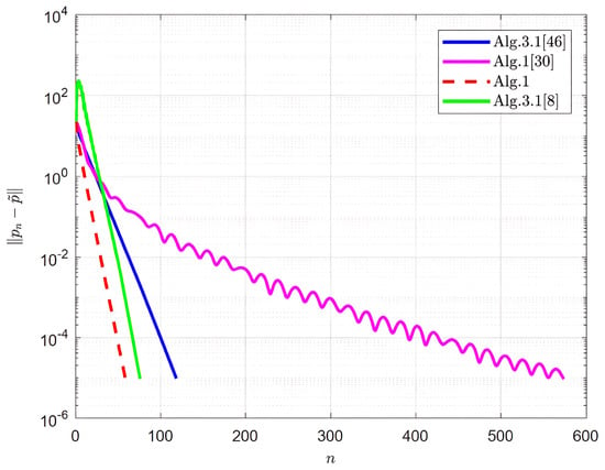
For Algorithm 3.1 [46], we take , , , and The corresponding results are reported in Table 1 and Figure 1, Figure 2 and Figure 3.
Table 1.
Comparison of Algorithm 3.1 [8], Algorithm 1 [30], Algorithm 3.1 [46] and Algorithm 1 for Example 1.
Figure 1.
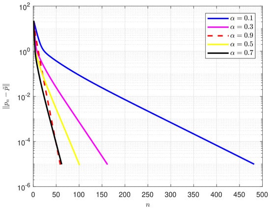
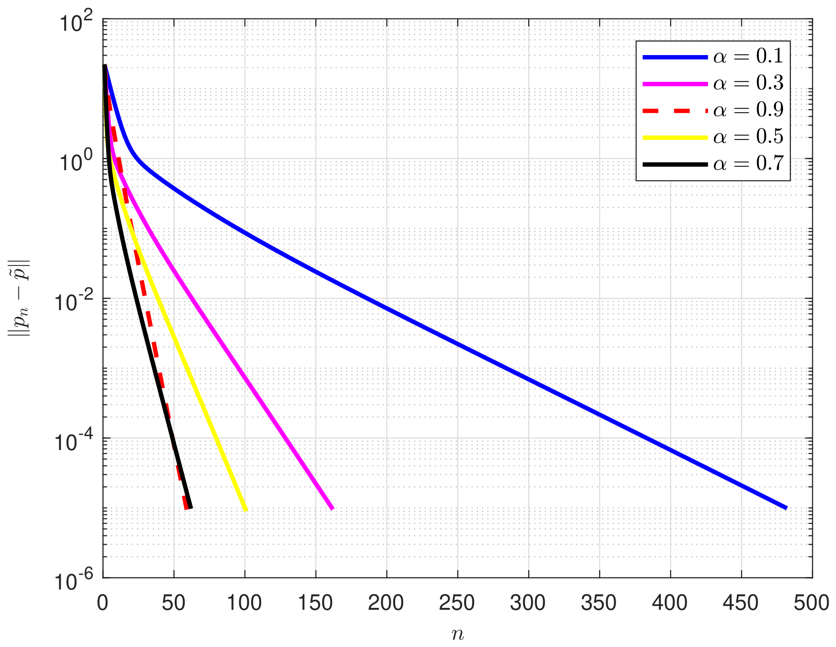
The sensitivity analysis of for Algorithm 1 and number of iterations for Example 1.
Figure 2.
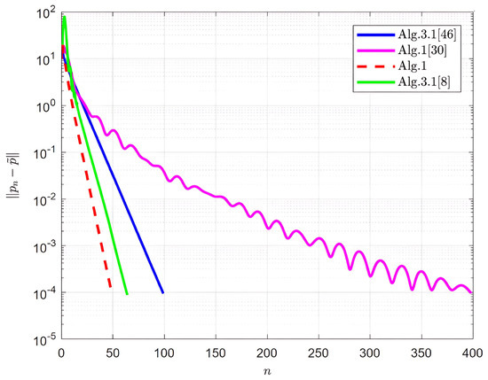
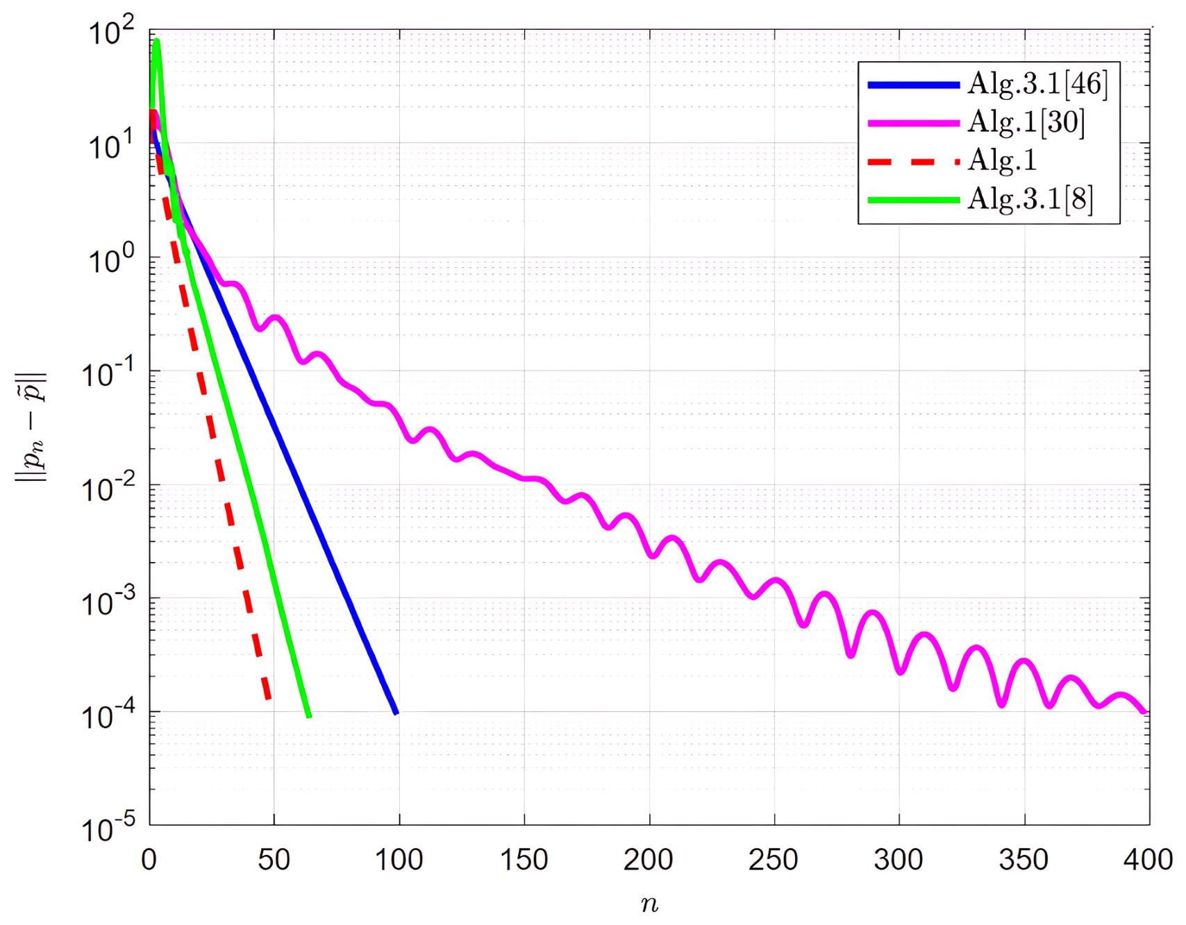
Number of iterations for Example 1 (, ).
Figure 3.
Number of iterations for Example 1 (, ).
Remark 3.
In Figure 1, we take the case , to test the effectiveness of Algorithm 1 by using different α. We obviously observe that the parameter α of our proposed algorithm (Algorithm 1) has an important impact on the numerical results. More specifically, the number of iterations is the lowest when Additionally, when , our proposed algorithm behaves well.
Remark 4.
As shown in Table 1, as well as Figure 2 and Figure 3, Algorithm 1, Algorithm 3.1 [8], Algorithm 1 [30] and Algorithm 3.1 [46] are Alg.1, Alg.3.1 [8], Alg.1 [30] and Alg.3.1 [46], respectively. All algorithms have a fast convergence rate. Especially, our proposed algorithm (Algorithm 1) needs fewer iterative numbers and less time than Algorithm 3.1 [8], Algorithm 1 [30] and Algorithm 3.1 [46] under different m and ε.
Example 2.
LASSO problem [7,23]. In this example, we introduce the following LASSO problem.
where , and This problem is devoted to finding a sparse solution of the SFP. The sampling matrice A is produced by a standard normal distribution with mean zero and unit variance. The truly sparse signal is built by distributing W nonzero elements uniformly at random in the interval while the rest is kept zero. The sample data .
In consideration of the SFP, we define and . We suggest the subgradient projection, because of the fact there has no closed-form expression for the projection of a closed convex set C. Let and
where . Additionally, the orthogonal projection of a point onto can be achieved by
The subdifferential at is
Additionally, we initialize the algorithms at the original and define
We test all methods under the same iteration error for different and limit the number of iterations to 5000, and the corresponding results are reported in Table 2.
Table 2.
Comparison of Algorithm 3.1 [8], Algorithm 1 [30], Algorithm 3.1 [46], and Algorithm 1 for Example 2.
The second problem is the recovery of the signal when , matrix A is randomly obtained with independent samples of standard Gaussian distribution. The original signal contains 150 randomly placed spikes. The initial point , we adopt the following mean square error for measuring the restoration accuracy:
For Algorithm 1 [30], we adopt , , and
where , which is suggested in [30].
As in [8], we set , , the inertial parameter , where ρ is the parameter in the linesearch for Algorithm 3.1 [8].
For Algorithm 1, we select , , , and . Additionally, is defined as in Algorithm 1 [30].
For Algorithm 3.1 [46], we take , , , and .
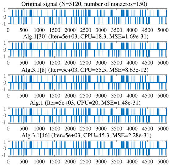
The corresponding results are reported in Table 2 and Figure 4, and Figure 4 provides numerical results we achieved for the original signal, MSE, and CPU time.
Figure 4.
Comparison of signal processing.
Remark 5.
In Figure 4, Algorithm 1, Algorithm 3.1 [8], Algorithm 1 [30] and Algorithm 3.1 [46] are Alg.1, Alg.3.1 [8], Alg.1 [30] and Alg.3.1 [46], respectively. From Table 2 and Figure 4, we see that all algorithms solve LASSO problems efficiently. In detail, our proposed algorithm (Algorithm 1) shows that the value of is smaller than the other compared algorithms. For the running time of all algorithms, Algorithm 1 behaves better than Algorithm 3.1 [8] and Algorithm 3.1 [46]; however, its time somewhat runs longer than Algorithm 1 [30] by testing the different cases.
7. Conclusions
We combine the inertial technique, new stepsize rules, the viscosity algorithm with linearized splitting algorithm for solving split variational inclusion problems, and we obtain its weak and strong convergence in real Hilbert spaces. Further, we extend our obtained results to split minimization problems and split feasibility problems. Finally, we make several experiments, which shows the advantages of our given algorithm.
8. Discussion
Compared with the linear splitting method in [30], our work has three important improvements. First, the new adaptive stepsize avoids zero-value stagnation and guarantees a positive lower bound. Second, the modified proximal term expands the feasible range of parameters from to for better numerical stability. Third, we introduce the viscosity algorithm to discuss the strong convergence in real Hilbert space. Further, we try to apply our proposed algorithm to the large-scale engineering optimization.
Author Contributions
Conceptualization, Q.Z.; methodology, Q.Z. and X.M.; software, Q.Z. and X.M.; formal analysis, Q.Z. and X.M.; investigation, Q.Z.; resources, Q.Z.; data curation, Q.Z.; writing—original draft preparation, Q.Z.; writing—review and editing, Q.Z. and X.M.; supervision, Q.Z. and X.M.; funding acquisition, Q.Z. and X.M. All authors have read and agreed to the published version of the manuscript.
Funding
The first author was supported by Qing Lan Project, and Suqian Sci Tech Program (No. M202206), the second author was supported by the National Natural Science Foundation of China (No. 12172266) and the Fundamental Research Program of Shanxi Province, China (No. 202303021222208).
Data Availability Statement
Data is contained within the article.
Conflicts of Interest
The authors declare no conflicts of interest.
References
- Moudafi, A. Split monotone variational inclusions. J. Optim. Theory Appl. 2011, 150, 275–283. [Google Scholar] [CrossRef] [Scilit]
- Kazmi, K.R.; Rizvi, S.H. An iterative method for split variational inclusion problem and fixed point problem for a nonexpansive mapping. Optim. Lett. 2014, 8, 1113–1124. [Google Scholar] [CrossRef] [Scilit]
- Arfat, Y.; Iyiola, O.; Wickramasinghe, M.; Kumam, P.; Khan, M.A.A. An inertia based viscosity type regularized splitting scheme for finding common solutions of split monotone variational inclusion and fixed point problems. Ann. Oper. Res. 2026. [Google Scholar] [CrossRef] [Scilit]
- Chuang, C.S. Hybrid inertial proximal algorithm for the split variational inclusion problem in Hilbert spaces with applications. Optimization 2017, 66, 777–792. [Google Scholar] [CrossRef] [Scilit]
- Sitthithakerngkiet, K.; Deepho, J.; Martinez-Moreno, J.; Kuman, P. Convergence analysis of a general iterative algorithm for finding a common solution of split variational inclusion and optimization problems. Numer. Algorithms 2018, 79, 801–824. [Google Scholar] [CrossRef] [Scilit]
- Thong, D.; Dung, V.; Cho, Y. A new strong convergence for solving split variational inclusion problems. Numer. Algorithms 2020, 86, 565–591. [Google Scholar] [CrossRef] [Scilit]
- Tibshirani, R. Regression shrinkage and selection via the Lasso. J. R. Stat. Soc. Ser. B 1996, 58, 267–288. [Google Scholar] [CrossRef] [Scilit]
- Kesornprom, S.; Cholamjiak, P. Proximal type algorithms involving linesearch and inertial technique for split variational inclusion problem in hilbert spaces with applications. Optimization 2019, 68, 2369–2395. [Google Scholar] [CrossRef] [Scilit]
- Censor, Y.; Bortfeld, T.; Martin, B.; Trofmov, A. A unifed approach for inversion problems in intensity-modulated radiation therapy. Phys. Med. Biol. 2006, 51, 2353–2365. [Google Scholar] [CrossRef] [Scilit] [PubMed]
- Combettes, P.L. The convex feasibility problem in image recovery. In Advances in Imaging and Electron Physics; Hawkes, P., Ed.; Academic Press: New York, NY, USA, 1996; pp. 155–270. [Google Scholar]
- Censor, Y.; Elfving, T. A multiprojection algorithm using Bregman projection in a product space. Numer. Algorithms 1994, 8, 221–239. [Google Scholar] [CrossRef] [Scilit]
- Wang, Z.; Lei, Z.; Long, X.; Chen, Z. A modified Tseng splitting method with double inertial steps for solving monotone inclusion problems. J. Sci. Comput. 2023, 96, 92. [Google Scholar] [CrossRef] [Scilit]
- Zhao, Y.; Tian, P.; Wu, D. An iterative method for solving split variational inclusion problem and variational inequality problem constrained by a common fixed point problem. J. Inequal. Appl. 2026, 2026, 71. [Google Scholar] [CrossRef] [Scilit]
- Arfat, Y.; Grad, S.; Tammer, C.; Kumam, P.; Khan, M.A.A. Solving split monotone variational inclusion problems via a relaxed-inertial self-adaptive regularized splitting algorithm. Numer. Algorithms 2026. [Google Scholar] [CrossRef] [Scilit]
- Byrne, C.; Censor, Y.; Gibali, A. Weak and strong convergence of algorithms for the split common null point problem. J. Nonlinear Convex Anal. 2011, 13, 759–775. [Google Scholar]
- López, G.; Martin, V.; Wang, F.; Xu, H.K. Solving the split feasibility problem without prior knowledge of matrix norms. Inverse Probl. 2012, 28, 085004. [Google Scholar] [CrossRef] [Scilit]
- Alvarez, F. Weak convergence of a relaxed and inertial hybrid projection-proximal point algorithm for maximal monotone operators in Hilbert spaces. SIAM J. Optim. 2004, 14, 773–782. [Google Scholar] [CrossRef] [Scilit]
- Polyak, B.T. Some methods of speeding up the convergence of iteration methods. USSR Comput. Math. Math. Phys. 1964, 4, 1–17. [Google Scholar] [CrossRef] [Scilit]
- Ma, X.; Liu, H.; Li, X. The iterative method for solving the proximal split feasibility problem with an application to LASSO problem. Comp. Appl. Math. 2022, 41, 5. [Google Scholar]
- Khairoowala, M.U.; Husain, S.; Furkan, M. An iterative algorithm for split variational inclusion, a system of variational inequalities and fixed point problems. J. Anal. 2025, 33, 3027–3049. [Google Scholar] [CrossRef] [Scilit]
- Li, H.; Wang, X.; Wang, F. Projection and contraction method with double inertial steps for quasi-monotone variational inequalities. Optimization 2025, 74, 1643–1674. [Google Scholar] [CrossRef] [Scilit]
- Yao, Y.; Iyiola, O.S.; Shehu, Y. Subgradient extragradient method with double inertial steps for variational inequalities. J. Sci. Comput. 2022, 90, 71. [Google Scholar] [CrossRef] [Scilit]
- Ma, X.; Liu, H.; Li, X. Two optimization approaches for solving split variational inclusion problems with applications. J. Sci. Comput. 2022, 91, 58. [Google Scholar] [CrossRef] [Scilit]
- Chang, X.; Yang, J. A golden ratio primal-dual algorithm for structured convex optimization. J. Sci. Comput. 2021, 87, 47. [Google Scholar] [CrossRef] [Scilit]
- Chang, X.; Yang, J.; Zhang, H. Golden ratio primal-dual algorithm with linesearch. SIAM J. Optim. 2022, 32, 1584–1613. [Google Scholar] [CrossRef] [Scilit]
- Rao, N.; Farid, M.; Jha, N.K. Szász-integral operators linking general-Appell polynomials and approximation. AIMS Math. 2025, 10, 13836–13854. [Google Scholar] [CrossRef] [Scilit]
- Dong, Q.L.; Cho, Y.J.; Rassias, T.M. General inertial Mann algorithms and their convergence analysis for nonexpansive mappings. Appl. Nonlinear Anal. 2018, 134, 175–191. [Google Scholar] [CrossRef] [Scilit]
- Nesterov, Y. A method for solving the convex programming problem with convergence rate O(1/k2). Dokl. Akad. Nauk. SSSR 1983, 269, 543–547. [Google Scholar]
- Thong, D.V. Convergence analysis of a self-adaptive inertial subgradient extragradient method for non-monotone variational inequalities with non-Lipschitz continuous mappings. Numer. Algorithms 2026. [Google Scholar] [CrossRef] [Scilit]
- Cholamjiak, P.; Suantai, S.; Kesornprom, S. Linearized splitting algorithm with inertial extrapolation for solving split variational inclusion problem and applications. Optimization 2025, 75, 1007–1029. [Google Scholar] [CrossRef] [Scilit]
- Xu, S.; Li, S.; Yao, J.C. Four double inertial algorithms for variational inequalities with fixed point constraints: Theory and signal processing applications. Numer. Algorithms 2026. [Google Scholar] [CrossRef] [Scilit]
- Wen, D.; Li, Q.; Zhang, H. A new proximal-type regularization algorithm for split monotone variational inclusions with applications. Comp. Appl. Math. 2026, 45, 373. [Google Scholar] [CrossRef] [Scilit]
- Dey, S.; Izuchukwu, C.; Taiwo, A.; Reich, S. New iterative algorithms for solving split variational inclusions. J. Glob. Optim. 2025, 91, 587–609. [Google Scholar] [CrossRef] [Scilit]
- Chai, Z.; Li, Y.; Han, Y.; Zhu, S. Recommendation System Based on Singular Value Decomposition and Multi-Objective Immune Optimization. IEEE Access 2019, 7, 6060–6071. [Google Scholar] [CrossRef] [Scilit]
- Tian, C.; Chen, Y. image segmentation and denoising algorithm based on partial differential equations. IEEE Sens. J. 2020, 20, 11935–11942. [Google Scholar] [CrossRef] [Scilit]
- Tian, C.; Chang, K.; Chen, J. Application of hyperbolic partial differential equations in global optimal scheduling of UAV. Alex. Eng. 2020, 59, 2283–2289. [Google Scholar] [CrossRef] [Scilit]
- Oikonomidis, K.A.; Bodard, A.; Laude, E.; Patrinos, P. Global convergence analysis of the power proximal point and augmented Lagrangian method. Comput. Optim. Appl. 2025, 93, 617–649. [Google Scholar] [CrossRef] [Scilit]
- Marino, G.; Xu, H.K. Convergence of generalized proximal point algorithm. Commun. Pure Appl. Anal. 2004, 3, 791–808. [Google Scholar] [CrossRef] [Scilit]
- Takahashi, W. Nonlinear Functional Analysis-Fixed Point Theory and Its Applications; Yokohama Publishers: Yokohama, Japan, 2000. [Google Scholar]
- Osilike, M.O.; Aniagbosor, S.C. Weak and strong convergence theorems for fixed points of asymptotically nonexpansive mappings. Math. Comput. Model. 2000, 32, 1181–1191. [Google Scholar] [CrossRef] [Scilit]
- Saejung, S.; Yotkaew, P. Approximation of zeros of inverse strongly monotone operators in Banach spaces. Nonlinear Anal. Theory Methods Appl. 2012, 75, 742–750. [Google Scholar] [CrossRef] [Scilit]
- Tang, Y.; Gibali, A. New self-adaptive step size algorithms for solving split variational inclusion problems and its applications. Numer. Algorithms 2020, 83, 305–331. [Google Scholar] [CrossRef] [Scilit]
- Takahashi, W.; Xu, H.K.; Yao, J.C. Iterative methods for generalized split feasibility problem in Hilbert spaces. Set. Valued Var. Anal. 2015, 23, 205–221. [Google Scholar] [CrossRef] [Scilit]
- Ceng, L.; Ansari, Q.; Yao, J. An extragradient method for solving split feasibility and fixed point problems. Comput. Math. Appl. 2012, 64, 633–642. [Google Scholar] [CrossRef] [Scilit]
- Long, L.; Thong, D.; Dng, V. New algorithms for the split variational inclusion problems and application to split feasibility problems. Optimization 2019, 68, 2339–2367. [Google Scholar] [CrossRef] [Scilit]
- Suantai, S.; Cholamjiak, P.; Inkrong, P.; Kesornprom, S. A fast contraction algorithm using two inertial extrapolations for variational inclusion problem and data classification. Carpath. J. Math. 2024, 40, 737–752. [Google Scholar] [CrossRef] [Scilit]

Disclaimer/Publisher’s Note: The statements, opinions and data contained in all publications are solely those of the individual author(s) and contributor(s) and not of MDPI and/or the editor(s). MDPI and/or the editor(s) disclaim responsibility for any injury to people or property resulting from any ideas, methods, instructions or products referred to in the content. |
© 2026 by the authors. Licensee MDPI, Basel, Switzerland. This article is an open access article distributed under the terms and conditions of the Creative Commons Attribution (CC BY) license.