A Novel Shrinkage Class for the Negative Binomial Regression Model: Theory, Simulation, and Healthcare Application in Saudi Arabia

Abstract

Count data are widely encountered in many scientific fields, particularly in healthcare and epidemiology. One of the most commonly used approaches for analyzing such data is the negative binomial regression model (NBRM), due to its simplicity and effectiveness in modeling event frequencies. Despite its popularity, the presence of severe multicollinearity among explanatory variables can substantially inflate the variance of parameter estimates and reduce the reliability of statistical inference. To address this issue, this study proposes an improved shrinkage estimator for the NBRM, referred to as a novel class of negative binomial Liu-type estimator. The proposed estimator combines the advantages of ridge regression and the Liu estimator, aiming to reduce estimation variance while maintaining stable parameter estimates under conditions of multicollinearity. The proposed estimator is compared with the traditional maximum likelihood estimator, as well as existing ridge and Liu-type estimators, using performance measures such as mean squared error. Its performance is evaluated through extensive Monte Carlo simulation experiments under different levels of multicollinearity and sample sizes. The simulation results demonstrate that the proposed estimator provides more accurate and stable estimates than the competing methods, particularly in the presence of high multicollinearity. To illustrate the practical applicability of the proposed approach, the method is applied to a real-world healthcare dataset related to COVID-19 cases in the Kingdom of Saudi Arabia. The empirical results confirm the effectiveness of the proposed estimator in improving estimation accuracy and model stability when modeling multivariate healthcare count data. Overall, the proposed estimator offers a useful alternative for modeling multicollinear healthcare count data and enhances the reliability of statistical analysis in applied health research.

1. Introduction

Count data, recorded as non-negative integers, often exhibit high right skewness. When this occurs, it violates the assumption of normality that classical linear regression relies upon. Due to this absence of normality, the application of these models is unjustified and will likely yield biased or inefficient estimates. Hence, multiple regression methods have been created specifically to handle the regression of count data. Some of the most common methods for this are Poisson regression, negative binomial regression model (NBRM), and extensions of these that handle many zero outcomes, such as hurdle, zero-inflated, and zero-truncated models [1,2]. The primary issue with these models is known as overdispersion, which occurs when the variance of the data set exceeds the mean. This creates problems for the Poisson model because one of its foundational assumptions no longer holds, and as a result, standard errors are likely to be underestimated, and many erroneous conclusions may be drawn [3].

The NBRM provides a viable alternative for overdispersed count data. In contrast with regression models built on the Poisson distribution, NBRM assumes the response variable is count data and follows a negative binomial distribution. It connects the log of the mean count with a linear combination of the independent variables. Because the model accommodates additional levels of variation, NBRM is valuable in a number of fields, including econometrics, biostatistics, healthcare, actuarial science, and education. NBRM is advantageous in instances where empirical count data demonstrate chronic overdispersion. In these cases, other models provide limited utility. The NBRM refines estimation and improves the quality of prediction by accounting for overdispersion in count data [4,5].

Individually assessing parameter estimates under a multiple regression analysis can be difficult due to multicollinearity, which describes the interconnectedness of the explanatory variables [6,7,8]. The detrimental impact of multicollinearity becomes apparent when estimating unknown parameters of a regression model and makes the process of applying MLE to NBRMs exceptionally difficult. Månsson and Shukur [9] suggest that the detrimental impact of multicollinearity on MLE means that the constraints on the analysis increase. The effects of multicollinearity on the analysis of regression models include inflated variances and increased standard errors (SE) of the regression parameters. These effects can result in parameter estimates that are inconsistent with the underlying theory. Furthermore, when multicollinearity is pronounced, several essential statistics of the classic theory (t-ratios, F-statistics, etc.) may even lose their significance, which impacts the overall hypothesis testing. This compromises the findings of a multivariate regression analysis.

Hoerl and Kennard [10] introduced the ridge regression estimator to tackle the multicollinearity issue in the multiple linear regression framework by adding a positive constant to the variance–covariance matrix, which was known as the ridge parameter. Extensive research has been conducted on how to choose the ridge parameter (see, e.g., Alkhamisi and Shukur [11], Alkhamisi et al. [12], Kibria [13], Algamal [14], Khalaf and Shukur [15], and Muniz and Kibria [16]), and it has been proven efficient through numerous simulation studies. Liu proposed another multicollinearity estimator [17], which is different from the ridge regression estimator in the sense that the Liu estimator uses a shrinkage parameter (d) in its linear structure. Since then, numerous estimators have been developed, which include the Liu-type estimator [18], Özkale and Kaciranlar’s estimator [19], the adjusted Liu estimator [20], Dawoud and Kibria’s estimator [21], the modified ridge-type estimator [22], the Kibria–Lukman estimator [23], and recently a hybrid-type estimator [24]. Works have also been carried out to extend Liu-type estimators under various regression models. Kurnaz and Akay [25] derived an extended family of Liu-type estimators under a linear regression model. Their study was later extended to generalized linear models (GLMs). Kurnaz and Akay [26] used the idea of Liu-type estimators under logistic regression, while Ertan et al. [27] extended it to the Bell regression model. Very recently, Alghamdi et al. [28] extended the same to the Poisson–inverse Gaussian regression model, while Almulhim et al. [29] extended it to the Conway–Maxwell–Poisson regression model.

In the case of the NBRM, several biased estimators have been introduced. Mansson [30,31] was the first to consider the ridge and Liu estimators in the NBRM. Later on, Asar [32] derived a Liu-type estimator for the model. Further contributions were made by Kandemir Çetinkaya and Kaçıranlar [33], who proposed the Özkale–Kaçıranlar estimator as an alternative shrinkage approach. Building on these developments, Jabur et al. [34] introduced a jackknifed Liu-type estimator to enhance estimation accuracy. More recently, Tuba and Haydar [35] presented the Kibria–Lukman estimator along with its jackknife variant, Ismael and Algamal [36] developed a new shrinkage estimator, Rashad [37] presented a generalized ridge estimator, and Alobaidi et al. [38] defined a new ridge estimator.

Despite existing studies, the need for a more flexible estimator to handle multicollinearity, particularly in the context of the NBRM, necessitates further research. This paper presents a novel class of Liu-type estimators designed to address the multicollinearity problem within the context of the NBRM, providing greater parameter stability and reducing both MSE and SE. We refer to this as a new class of negative binomial Liu-type estimators. In order to illustrate the benefits of our proposed estimator, we carry out a theoretical analysis in which we compare our proposed estimator with existing ones using MMSE and SMSE. Moreover, we perform Monte Carlo simulations in which we consider SMSE and bias as the primary evaluation criteria. We also consider the applicability of the estimator by working with two real-life datasets, one of which contains COVID-19 data from Saudi Arabia. Our findings indicate the superiority of the proposed estimator compared to classical approaches in the presence of multicollinearity.

The rest of this paper is organized as follows: Section 2 presents the building blocks of the NBRM and a discussion of its methodological paradigm. In Section 3, we propose a set of biased estimators for the NBRM and provide a thorough mathematical exposition for each estimator, along with a theoretical assessment of each based on the MMSE and the SMSE. Section 4 presents a description of the design of the Monte Carlo simulation and reports the principal outcomes of the study. In Section 5, we present several case studies to demonstrate the estimator of interest. Finally, in Section 6, we provide a synthesis of the findings, highlight some shortcomings, and map out some possible future research avenues.

2. Methodology

The NBRM can be described as a versatile and strong statistical tool used in the modeling of count data, especially if $y_i$ takes on non-negative integers. NBRM assumes that $y_i$ is distributed as a negative binomial random variable, such that $y_i\sim \mathrm{NB}({\mu }_i,{\mu }_i+\vartheta {\mu }_i^2)$, where ${\mu }_i$ is the mean parameter and ${\mu }_i=exp\left(x_i^{\prime }\beta \right)$. Here, $x_i$ stands for the i-th row of the design matrix X of size $n\times p$, which includes an intercept as well as $(p-1)$ regressors, and $\beta$ stands for the associated regression parameters. The probability mass function of $y_i$ can be described as

$$\begin{array}{c}\hfill P\left(y_i\right|x_i)={\displaystyle \frac{\mathrm{\Gamma }({\vartheta }^{-1}+y_i)}{\mathrm{\Gamma }\left({\vartheta }^{-1}\right)\mathrm{\Gamma }(1+y_i)}}{\left({\displaystyle \frac{{\vartheta }^{-1}}{{\vartheta }^{-1}+{\mu }_i}}\right)}^{{\vartheta }^{-1}}{\left({\displaystyle \frac{{\mu }_i}{{\vartheta }^{-1}+{\mu }_i}}\right)}^{y_i},\end{array}$$

(1)

where $\vartheta =1/\delta$ is a dispersion parameter that governs the extent of overdispersion. Under this formulation, the conditional mean and variance of the response are expressed as

$$E\left(y_i\right|x_i)={\mu }_i,V\left(y_i\right|x_i)={\mu }_i(1+\vartheta {\mu }_i).$$

Estimation of the model parameters is typically carried out via maximum likelihood (MLE). The log-likelihood function, which incorporates the identity $log\left({\displaystyle \frac{\mathrm{\Gamma }({\vartheta }^{-1}+y_i)}{\mathrm{\Gamma }\left({\vartheta }^{-1}\right)}}\right)={\sum }_{j=0}^{y_i-1}log(j+{\vartheta }^{-1})$ [33], takes the form

$$\begin{array}{c}\hfill l(\vartheta ;\beta )={\displaystyle \sum _{i=1}^n}\left\{{\displaystyle \sum _{j=0}^{y_i-1}}log(j+{\vartheta }^{-1})-log(y_i!)-(y_i+{\vartheta }^{-1})log\left(1+\vartheta exp\left(x_i^{\prime }\beta \right)\right)+y_{i}log\left(\vartheta \right)+y_i{x}_i^{\prime }\beta \right\}.\end{array}$$

(2)

Differentiating this log-likelihood with respect to $\beta$ yields the score function

$$\begin{array}{c}\hfill S\left(\beta \right)={\displaystyle \frac{\partial l(\vartheta ;\beta )}{\partial \beta }}={\displaystyle \sum _{i=1}^n}{\displaystyle \frac{(y_i-exp\left(x_i^{\prime }\beta \right))}{1+\vartheta exp\left(x_i^{\prime }\beta \right)}}{x}_i.\end{array}$$

(3)

Since this equation is nonlinear in $\beta$, an iterative procedure such as the Newton–Raphson or Fisher scoring algorithm is employed. The updating scheme at iteration m is given by

$$\begin{array}{c}\hfill {\beta }^{\left(m\right)}={\beta }^{(m-1)}+I^{-1}\left({\beta }^{(m-1)}\right)S\left({\beta }^{(m-1)}\right),\end{array}$$

(4)

where $I\left({\beta }^{(m-1)}\right)$ denotes the Fisher information matrix, defined as

$$\begin{array}{c}\hfill I\left({\beta }^{(m-1)}\right)=X^{\prime }U\left({\beta }^{(m-1)}\right)X,U\left({\beta }^{(m-1)}\right)=\mathrm{diag}\left({\displaystyle \frac{{\mu }_i}{1+\vartheta {\mu }_i}}\right).\end{array}$$

(5)

This iterative process can be reformulated as a weighted least squares problem,

$$\begin{array}{c}\hfill X^{\prime }U\left({\beta }^{(m-1)}\right)X{\beta }^{\left(m\right)}=X^{\prime }U\left({\beta }^{(m-1)}\right)z\left({\beta }^{(m-1)}\right),\end{array}$$

(6)

where the adjusted dependent variable $z\left({\beta }^{(m-1)}\right)$ is defined as $z\left({\beta }^{(m-1)}\right)=log\left({\mu }_i\left({\beta }^{(m-1)}\right)\right)+{\displaystyle \frac{y_i-{\mu }_i\left({\beta }^{(m-1)}\right)}{{\mu }_i\left({\beta }^{(m-1)}\right)}}$. Upon convergence, the negative binomial maximum likelihood estimator (NBMLE) of $\beta$ is obtained as

$$\begin{array}{c}\hfill {\widehat{\beta }}_{\mathrm{NBMLE}}=W^{-1}{X}^{\prime }\widehat{U}\widehat{z}.\end{array}$$

(7)

where $W=X^{\prime }\widehat{U}X$. The asymptotic variance–covariance matrix of the NBMLE is given by the inverse of the Fisher information matrix,

$$\begin{array}{c}\hfill \mathrm{Cov}\left({\widehat{\beta }}_{\mathrm{NBMLE}}\right)=W^{-1}.\end{array}$$

(8)

To evaluate the estimator’s precision, the MMSE and the SMSE are commonly employed. These measures are defined as

$$\begin{array}{c}\hfill \mathrm{MMSE}\left({\widehat{\beta }}_{\mathrm{NBMLE}}\right)=\mathrm{\Gamma }{\mathrm{\Psi }}^{-1}{\mathrm{\Gamma }}^{\prime },\end{array}$$

(9)

$$\mathrm{SMSE}\left({\widehat{\beta }}_{\mathrm{NBMLE}}\right)=\mathrm{tr}\left(\mathrm{MMSE}({\widehat{\beta }}_{\mathrm{NBMLE}})\right)={\displaystyle \sum _{j=1}^p}{\displaystyle \frac{1}{{\psi }_j}},$$

(10)

where $\mathrm{tr}(·)$ denotes the trace operator. The matrix $\mathrm{\Psi }=\mathrm{\Gamma }W{\mathrm{\Gamma }}^{\prime }=\mathrm{diag}({\psi }_1,{\psi }_2,\dots ,{\psi }_p)$ contains the eigenvalues of W, and $\mathrm{\Gamma }$ is an orthogonal matrix whose columns are the corresponding eigenvectors. The quantity ${\psi }_j$ represents the j-th eigenvalue associated with the matrix W. Severe multicollinearity among the predictor variables results in an ill-conditioned weighted matrix. As a consequence, the variance of the NBMLE is substantially inflated, leading to estimated regression coefficients that are unstable, overly large in magnitude, and problematic for meaningful interpretation.

To mitigate the adverse effects of multicollinearity in NBRM, several biased estimators have been developed, each introducing shrinkage parameters to stabilize the estimates. Månsson [30] pioneered this line of research by proposing the negative binomial ridge regression estimator (NBRRE), which is defined as

$${\widehat{\beta }}_{\mathrm{NBRRE}}={(W+kI)}^{-1}W{\widehat{\beta }}_{\mathrm{NBMLE}},k>0,$$

(11)

where the ridge parameter k controls the degree of shrinkage and I is the identity matrix. This estimator reduces to the NBMLE when $k\to 0$.

Building upon this foundation, Månsson [31] introduced the negative binomial Liu regression estimator (NBLRE), which incorporates a different shrinkage mechanism,

$${\widehat{\beta }}_{\mathrm{NBLRE}}={(W+I)}^{-1}(W+dI){\widehat{\beta }}_{\mathrm{NBMLE}},0<d<1,$$

(12)

with the Liu parameter d typically constrained to the unit interval. Setting $d\to 1$ yields the NBMLE as a special case.

Asar [32] contributed a more flexible two-parameter approach, termed the negative binomial Liu-type estimator (NBLTE), expressed as

$${\widehat{\beta }}_{\mathrm{NBLTE}}={(W+kI)}^{-1}(W-dI){\widehat{\beta }}_{\mathrm{NBMLE}},-\infty <d<\infty ,k>0,$$

(13)

where k and d are the Liu-type parameters. This formulation encompasses the NBRRE when $d\to 0$ and reduces to the NBMLE when both shrinkage parameters are set to zero.

In a similar vein, Kandemir Çetinkaya and Kaçıranlar [33] adapted the estimator originally proposed by Özkale and Kaciranlar [19] to the negative binomial context, resulting in the negative binomial Özkale Kaciranlar estimator (NBOKE):

$${\widehat{\beta }}_{\mathrm{NBOKE}}={(W+kI)}^{-1}(W+kdI){\widehat{\beta }}_{\mathrm{NBMLE}},0<d<1,k>0,$$

(14)

where k and d are the Özkale Kaciranlar parameters. This estimator demonstrates notable flexibility: it simplifies to the NBLRE when $k\to 1$, to the NBRRE when $d\to 0$, and to the NBMLE when both parameters are zero.

For each of the estimators introduced in the preceding section, the associated MMSE and SMSE are provided below.

$$\begin{array}{c}\hfill \begin{array}{c}\hfill \mathrm{MMSE}\left({\widehat{\beta }}_{\mathrm{NBRRE}}\right)=\mathrm{\Gamma }{\mathrm{\Psi }}_k^{-1}\mathrm{\Psi }{\mathrm{\Psi }}_k^{-1}{\mathrm{\Gamma }}^{\prime }+k^2\mathrm{\Gamma }{\mathrm{\Psi }}_k^{-1}\delta {\delta }^{\prime }{\mathrm{\Psi }}_k^{-1}{\mathrm{\Gamma }}^{\prime },\end{array}\end{array}$$

(15)

$$\begin{array}{c}\hfill \begin{array}{c}\hfill \mathrm{SMSE}\left({\widehat{\beta }}_{\mathrm{NBRRE}}\right)={\displaystyle \sum _{j=1}^p}{\displaystyle \frac{{\psi }_j}{{({\psi }_j+k)}^2}}+k^2{\displaystyle \sum _{j=1}^p}{\displaystyle \frac{{\delta }_j^2}{{({\psi }_j+k)}^2}},\end{array}\end{array}$$

(16)

$$\mathrm{MMSE}\left({\widehat{\beta }}_{\mathrm{NBLRE}}\right)=\mathrm{\Gamma }{\mathrm{\Psi }}_1^{-1}{\mathrm{\Psi }}_d{\mathrm{\Psi }}^{-1}{\mathrm{\Psi }}_d{\mathrm{\Psi }}_1^{-1}{\mathrm{\Gamma }}^{\prime }+{(d-1)}^2\mathrm{\Gamma }{\mathrm{\Psi }}_1^{-1}\delta {\delta }^{\prime }{\mathrm{\Psi }}_1^{-1}{\mathrm{\Gamma }}^{\prime },$$

(17)

$$\begin{array}{c}\hfill \begin{array}{c}\hfill \mathrm{SMSE}\left({\widehat{\beta }}_{\mathrm{NBLRE}}\right)={\displaystyle \sum _{j=1}^p}{\displaystyle \frac{{(\psi }_j{+d)}^2}{{\psi }_j{({\psi }_j+1)}^2}}+{(d-1)}^2{\displaystyle \sum _{j=1}^p}{\displaystyle \frac{{\delta }_j^2}{{({\psi }_j+1)}^2}},\end{array}\end{array}$$

(18)

$$\mathrm{MMSE}\left({\widehat{\beta }}_{\mathrm{NBLTE}}\right)=\mathrm{\Gamma }{\mathrm{\Psi }}_k^{-1}{\mathrm{\Psi }}_{d_0}{\mathrm{\Psi }}^{-1}{\mathrm{\Psi }}_{d_0}{\mathrm{\Psi }}_k^{-1}{\mathrm{\Gamma }}^{\prime }+{(d+k)}^2\mathrm{\Gamma }{\mathrm{\Psi }}_k^{-1}\delta {\delta }^{\prime }{\mathrm{\Psi }}_k^{-1}{\mathrm{\Gamma }}^{\prime },$$

(19)

$$\begin{array}{c}\hfill \begin{array}{c}\hfill \mathrm{SMSE}\left({\widehat{\beta }}_{\mathrm{NBLTE}}\right)={\displaystyle \sum _{j=1}^p}{\displaystyle \frac{{(\psi }_j{-d)}^2}{{\psi }_j{({\psi }_j+k)}^2}}+{(d+k)}^2{\displaystyle \sum _{j=1}^p}{\displaystyle \frac{{\delta }_j^2}{{({\psi }_j+k)}^2}},\end{array}\end{array}$$

(20)

$$\mathrm{MMSE}\left({\widehat{\beta }}_{\mathrm{NBOKE}}\right)=\mathrm{\Gamma }{\mathrm{\Psi }}_k^{-1}{\mathrm{\Psi }}_{kd}{\mathrm{\Psi }}^{-1}{\mathrm{\Psi }}_{kd}{\mathrm{\Psi }}_k^{-1}{\mathrm{\Gamma }}^{\prime }+k^2{(d-1)}^2\mathrm{\Gamma }{\mathrm{\Psi }}_k^{-1}\delta {\delta }^{\prime }{\mathrm{\Psi }}_k^{-1}{\mathrm{\Gamma }}^{\prime },$$

(21)

$$\begin{array}{c}\hfill \begin{array}{c}\hfill \mathrm{SMSE}\left({\widehat{\beta }}_{\mathrm{NBOKE}}\right)={\displaystyle \sum _{j=1}^p}{\displaystyle \frac{{(\psi }_j{+kd)}^2}{{\psi }_j{({\psi }_j+k)}^2}}+k^2{(d-1)}^2{\displaystyle \sum _{j=1}^p}{\displaystyle \frac{{\delta }_j^2}{{({\psi }_j+k)}^2}},\end{array}\end{array}$$

(22)

where ${\mathrm{\Psi }}_k=\mathrm{diag}({\psi }_1+k,{\psi }_2+k,\dots ,{\psi }_p+k)$, ${\mathrm{\Psi }}_1=\mathrm{diag}({\psi }_1+1,{\psi }_2+1,\dots ,{\psi }_p+1)$, ${\mathrm{\Psi }}_d=\mathrm{diag}({\psi }_1+d,{\psi }_2+d,\dots ,{\psi }_p+d)$, ${\mathrm{\Psi }}_{d_0}=\mathrm{diag}({\psi }_1-d,{\psi }_2-d,\dots ,{\psi }_p-d)$, ${\mathrm{\Psi }}_{kd}=\mathrm{diag}({\psi }_1+kd,{\psi }_2+kd,\dots ,{\psi }_p+kd)$, and $\delta ={\mathrm{\Gamma }}^{\prime }{\widehat{\beta }}_{\mathrm{NBMLE}}$.

3. Proposed Estimator

This section proposes a new estimator for the NBRM with its statistical properties, demonstrates its superiority over conventional estimators in terms of efficiency, and discusses the selection of appropriate biasing parameters for the biasing estimator.

3.1. Negative Binomial Class of Liu-Type Estimator

Multicollinearity in the NBRMs remains inadequately addressed by existing single-parameter shrinkage estimators. The NBRRE stabilizes coefficient estimates by shrinking toward zero along a single parameter k, but its bias increases monotonically with k, forcing an unfavorable trade-off between variance reduction and bias inflation, particularly under severe collinearity. The NBLRE, by contrast, uses a bounded parameter $d\in (0,1)$ that controls shrinkage more conservatively, but this bounded range limits its capacity to handle cases where collinearity is extreme, and a larger shrinkage magnitude is required for stability. The NBLTE and the NBOKE both rely on two parameters, k and d, to balance the bias-variance trade-off; however, because d enters each estimator through a fixed functional form, neither is guaranteed to yield the optimal bias-variance balance across all degrees of multicollinearity. In other words, having two parameters increases flexibility relative to the single-parameter estimators, but the rigid relationship imposed between k and d in each case still restricts the estimator to a narrow subset of possible shrinkage behaviors, which may not correspond to the optimal solution for a given collinearity structure.

In this paper, we propose the negative binomial class of Liu-type estimators (NBCLTE), which offers greater efficiency than the existing estimators in addressing multicollinearity and achieves a lower SMSE by allowing the bias-correction term to vary continuously with the shrinkage parameter, rather than being fixed to a single predetermined form. The proposed estimator can be defined as follows:

$${\widehat{\beta }}_{\mathrm{NBCLTE}}={(W+kI)}^{-1}(W+f\left(k\right)I){\widehat{\beta }}^{*},k>0,$$

(23)

where k serves as a shrinkage parameter governing the estimator’s properties and ${\widehat{\beta }}^{*}$ denotes any consistent estimator of the coefficient vector $\beta$. The function $f\left(k\right)$ is assumed to be continuous with respect to k, offering flexibility in defining various estimator subclasses [25]. By specifying $f\left(k\right)$ as a linear function of the form $f\left(k\right)=ak+b$, where a and b are real constants, the proposed estimator in Equation (23) encompasses several well-known biased estimators as special cases. When ${\widehat{\beta }}^{*}$ is taken to be the NBMLE ${\widehat{\beta }}_{\mathrm{NBMLE}}$, the following special cases emerge:

• Setting $f\left(k\right)=k$ (i.e., $a=1,b=0$) yields the NBMLE: ${\widehat{\beta }}_{\mathrm{NBCLTE}}={\widehat{\beta }}_{\mathrm{NBMLE}}$.
• Choosing $f\left(k\right)=0$ (i.e., $a=0,b=0$) produces the NBRRE: ${\widehat{\beta }}_{\mathrm{NBCLTE}}={\widehat{\beta }}_{\mathrm{NBRRE}}$.
• With $f\left(1\right)=d$ (i.e., $a=-1,b=1+d$), the estimator reduces to the NBLRE: ${\widehat{\beta }}_{\mathrm{NBCLTE}}={\widehat{\beta }}_{\mathrm{NBLRE}}$.
• When $f\left(k\right)=dk$, (i.e., $a=d,b=0$) yields the NBOKE: ${\widehat{\beta }}_{\mathrm{NBCLTE}}={\widehat{\beta }}_{\mathrm{NBOKE}}$.
• When $f\left(1\right)=-k+b$, where the linear expression corresponds to the biasing parameter $-d$, the estimator simplifies to the NBLTR: ${\widehat{\beta }}_{\mathrm{NBCLTE}}={\widehat{\beta }}_{\mathrm{NBLTE}}$.

From these specializations, it is evident that the estimator defined in Equation (23) represents a broader class than the Liu-type estimator introduced earlier. In fact, the conventional Liu-type estimator can be regarded as a particular instance of this unified framework.

To facilitate theoretical comparisons, we derive the bias vector and variance–covariance matrix of the proposed estimator. These expressions are given by

$$\mathrm{Bias}\left({\widehat{\beta }}_{\mathrm{NBCLTE}}\right)=E\left({\widehat{\beta }}_{\mathrm{NBCLTE}}\right)-\beta =(f\left(k\right)-k)\mathrm{\Gamma }{\mathrm{\Psi }}_k^{-1}\delta ,$$

(24)

$$\begin{array}{c}\hfill \begin{array}{cc}\hfill \mathrm{Cov}\left({\widehat{\beta }}_{\mathrm{NBCLTE}}\right)& =E\left(\left[{\widehat{\beta }}_{\mathrm{NBCLTE}}-E\left({\widehat{\beta }}_{\mathrm{NBCLTE}}\right)\right]{\left[{\widehat{\beta }}_{\mathrm{NBCLTE}}-E\left({\widehat{\beta }}_{\mathrm{NBCLTE}}\right)\right]}^{\prime }\right)\hfill \\ \hfill & =\mathrm{\Gamma }{\mathrm{\Psi }}_k^{-1}{\mathrm{\Psi }}_{f\left(k\right)}{\mathrm{\Psi }}^{-1}{\mathrm{\Psi }}_{f\left(k\right)}{\mathrm{\Psi }}_k^{-1}{\mathrm{\Gamma }}^{\prime }.\hfill \end{array}\end{array}$$

(25)

Using these components, the MMSE and SMSE of ${\widehat{\beta }}_{\mathrm{NBCLTE}}$ are obtained as

$$\begin{array}{c}\hfill \begin{array}{cc}\hfill \mathrm{MSEM}\left({\widehat{\beta }}_{\mathrm{NBCLTE}}\right)& =\mathrm{Cov}\left({\widehat{\beta }}_{\mathrm{NBCLTE}}\right)+\mathrm{Bias}\left({\widehat{\beta }}_{\mathrm{NBCLTE}}\right)\mathrm{Bias}{\left({\widehat{\beta }}_{\mathrm{NBCLTE}}\right)}^{\prime }\hfill \\ \hfill & =\mathrm{\Gamma }{\mathrm{\Psi }}_k^{-1}{\mathrm{\Psi }}_{f\left(k\right)}{\mathrm{\Psi }}^{-1}{\mathrm{\Psi }}_{f\left(k\right)}{\mathrm{\Psi }}_k^{-1}{\mathrm{\Gamma }}^{\prime }+{(f\left(k\right)-k)}^2\mathrm{\Gamma }{\mathrm{\Psi }}_k^{-1}\delta {\delta }^{\prime }{\mathrm{\Psi }}_k^{-1}{\mathrm{\Gamma }}^{\prime },\hfill \end{array}\end{array}$$

(26)

$$\begin{array}{c}\hfill \begin{array}{cc}\hfill \mathrm{SMSE}\left({\widehat{\beta }}_{\mathrm{NBCLTE}}\right)& =\mathrm{tr}\left(\mathrm{MMSE}\left({\widehat{\beta }}_{\mathrm{NBCLTE}}\right)\right)\hfill \\ \hfill & ={\displaystyle \sum _{j=1}^p}{\displaystyle \frac{{({\psi }_j+f\left(k\right))}^2}{{\psi }_j{({\psi }_j+k)}^2}}+{(f\left(k\right)-k)}^2{\displaystyle \sum _{j=1}^p}{\displaystyle \frac{{\delta }_j^2}{{({\psi }_j+k)}^2}},\hfill \end{array}\end{array}$$

(27)

where ${\mathrm{\Psi }}_{f\left(k\right)}=\mathrm{diag}({\psi }_1+f\left(k\right),{\psi }_2+f\left(k\right),\dots ,{\psi }_p+f\left(k\right))$, and $\mathrm{tr}(·)$ denotes the trace operator. In Equation (27), the first term represents the asymptotic variance contribution, while the second term captures the squared bias introduced by the shrinkage procedure.

3.2. The Superiority of the Proposed Estimator

The theoretical derivations presented in this section rely on the following lemma, which establishes a fundamental condition for the positive definiteness of a matrix difference.

Lemma 1. 

Let B be a positive definite matrix, c a positive scalar, and γ a non-zero constant vector. Then the matrix $cB-\gamma {\gamma }^{\prime }$ is positive definite if and only if (iff) ${\gamma }^{\prime }{B}^{-1}\gamma <c$ [39].

Theorem 1. 

Let $R=\mathit{Bias}\left({\widehat{\beta }}_{\mathit{NBCLTE}}\right)$, the proposed estimator ${\widehat{\beta }}_{\mathit{NBCLTE}}$ outperforms ${\widehat{\beta }}_{\mathit{NBMLE}}$ iff $\mathit{MMSE}\left({\widehat{\beta }}_{\mathit{NBMLE}}\right)-\mathit{MMSE}\left({\widehat{\beta }}_{\mathit{NBCLTE}}\right)>0$, which holds under the sufficient assumptions $k>f\left(k\right)$ and $k>0$.

Proof. 

To establish the dominance condition, we first consider the difference between the MMSEs of the two estimators. Utilizing the expressions given in Equation (9) for the NBMLE and Equation (26) for the proposed estimator, this difference takes the form

$$\mathrm{MMSE}\left({\widehat{\beta }}_{\mathrm{NBMLE}}\right)-\mathrm{MMSE}\left({\widehat{\beta }}_{\mathrm{NBCLTE}}\right)=\mathrm{\Gamma }({\mathrm{\Psi }}^{-1}-{\mathrm{\Psi }}_k^{-1}{\mathrm{\Psi }}_{f\left(k\right)}{\mathrm{\Psi }}^{-1}{\mathrm{\Psi }}_{f\left(k\right)}{\mathrm{\Psi }}_k^{-1}){\mathrm{\Gamma }}^{\prime }-R{R}^{\prime }.$$

(28)

An equivalent expression in terms of SMSE can be written as

$$\mathrm{SMSE}\left({\widehat{\beta }}_{\mathrm{NBMLE}}\right)-\mathrm{SMSE}\left({\widehat{\beta }}_{\mathrm{NBCLTE}}\right)=\mathrm{\Gamma }\mathrm{diag}\left({\displaystyle \frac{1}{{\psi }_j}}-{\displaystyle \frac{{({\psi }_j+f\left(k\right))}^2}{{\psi }_j{({\psi }_j+k)}^2}}\right){\mathrm{\Gamma }}^{\prime }-R{R}^{\prime }.$$

(29)

For the matrix difference in (28) to be positive definite, it is sufficient that the diagonal matrix $({\mathrm{\Psi }}^{-1}-{\mathrm{\Psi }}_k^{-1}{\mathrm{\Psi }}_{f\left(k\right)}{\mathrm{\Psi }}^{-1}{\mathrm{\Psi }}_{f\left(k\right)}{\mathrm{\Psi }}_k^{-1})$ be positive definite. This condition holds when each diagonal element satisfies: ${({\psi }_j+k)}^2-{({\psi }_j+f\left(k\right))}^2>0$ or equivalently: $(k-f\left(k\right))(2{\psi }_j+k+f\left(k\right))>0$. Given the parameter constraints $k>f\left(k\right)$, the inequality above is satisfied for all j. The proof is then completed by applying Lemma 1.    □

Theorem 2. 

Let $R_1=\mathit{Bias}\left({\widehat{\beta }}_{\mathit{NBRRE}}\right)$ and $R=\mathit{Bias}\left({\widehat{\beta }}_{\mathit{NBCLTE}}\right)$, the proposed estimator ${\widehat{\beta }}_{\mathit{NBCLTE}}$ outperforms ${\widehat{\beta }}_{\mathit{NBRRE}}$ iff $\mathit{MMSE}\left({\widehat{\beta }}_{\mathit{NBRRE}}\right)-\mathit{MMSE}\left({\widehat{\beta }}_{\mathit{NBCLTE}}\right)>0$, which holds under the sufficient assumptions $-2{\psi }_j<f\left(k\right)<0$ and $k>0$.

Proof. 

To establish the dominance condition, we first consider the difference between the MMSEs of the two estimators. Utilizing the expressions given in Equation (15) for the NBRRE and Equation (26) for the proposed estimator, this difference takes the form

$$\mathrm{MMSE}\left({\widehat{\beta }}_{\mathrm{NBRRE}}\right)-\mathrm{MMSE}\left({\widehat{\beta }}_{\mathrm{NBCLTE}}\right)=\mathrm{\Gamma }({\mathrm{\Psi }}_k^{-1}\mathrm{\Psi }{\mathrm{\Psi }}_k^{-1}-{\mathrm{\Psi }}_k^{-1}{\mathrm{\Psi }}_{f\left(k\right)}{\mathrm{\Psi }}^{-1}{\mathrm{\Psi }}_{f\left(k\right)}{\mathrm{\Psi }}_k^{-1}){\mathrm{\Gamma }}^{\prime }+R_1{R}_1^{\prime }-R{R}^{\prime }.$$

(30)

An equivalent expression in terms of SMSE can be written as

$$\begin{array}{c}\hfill \begin{array}{cc}\hfill \mathrm{SMSE}\left({\widehat{\beta }}_{\mathrm{NBRRE}}\right)-\mathrm{SMSE}\left({\widehat{\beta }}_{\mathrm{NBCLTE}}\right)=& \mathrm{\Gamma }\mathrm{diag}\left({\displaystyle \frac{{\psi }_j}{{({\psi }_j+k)}^2}}-{\displaystyle \frac{{({\psi }_j+f\left(k\right))}^2}{{\psi }_j{({\psi }_j+k)}^2}}\right){\mathrm{\Gamma }}^{\prime }+R_1{R}_1^{\prime }-R{R}^{\prime }.\hfill \end{array}\end{array}$$

(31)

For the matrix difference in (30) to be positive definite, it is sufficient that the diagonal matrix $({\mathrm{\Psi }}_k^{-1}\mathrm{\Psi }{\mathrm{\Psi }}_k^{-1}-{\mathrm{\Psi }}_k^{-1}{\mathrm{\Psi }}_{f\left(k\right)}{\mathrm{\Psi }}^{-1}{\mathrm{\Psi }}_{f\left(k\right)}{\mathrm{\Psi }}_k^{-1})$ be positive definite. This condition holds when each diagonal element satisfies: ${\psi }_j^2-{({\psi }_j+f\left(k\right))}^2>0$ or equivalently $-2{\psi }_j<f\left(k\right)<0$. Given the parameter constraints $k>0$, the inequality above is satisfied for all j. The proof is then completed by applying Lemma 1.    □

Theorem 3. 

Let $R=\mathit{Bias}\left({\widehat{\beta }}_{\mathit{NBCLTE}}\right)$ and $R_2=\mathit{Bias}\left({\widehat{\beta }}_{\mathit{NBLRE}}\right)$, the proposed estimator ${\widehat{\beta }}_{\mathit{NBCLTE}}$ outperforms ${\widehat{\beta }}_{\mathit{NBLRE}}$ iff $\mathit{MMSE}\left({\widehat{\beta }}_{\mathit{NBLRE}}\right)-\mathit{MMSE}\left({\widehat{\beta }}_{\mathit{NBCLTE}}\right)>0$, which holds under the sufficient assumptions $-{\displaystyle \frac{{\psi }_j(k+d+1)+dk}{{\psi }_j+1}}<f\left(k\right)<{\displaystyle \frac{{\psi }_j(k+d-1)+dk}{{\psi }_j+1}}$, $k>0$, and $0<d<1$.

Proof. 

To establish the dominance condition, we first consider the difference between the MMSEs of the two estimators. Utilizing the expressions given in Equation (17) for the NBLRE and Equation (26) for the proposed estimator, this difference takes the form

$$\begin{array}{cc}\hfill \mathrm{MMSE}\left({\widehat{\beta }}_{\mathrm{NBLRE}}\right)-\mathrm{MMSE}\left({\widehat{\beta }}_{\mathrm{NBCLTE}}\right)=& \mathrm{\Gamma }({\mathrm{\Psi }}_1^{-1}{\mathrm{\Psi }}_d{\mathrm{\Psi }}^{-1}{\mathrm{\Psi }}_d{\mathrm{\Psi }}_1^{-1}-{\mathrm{\Psi }}_k^{-1}{\mathrm{\Psi }}_{f\left(k\right)}{\mathrm{\Psi }}^{-1}{\mathrm{\Psi }}_{f\left(k\right)}{\mathrm{\Psi }}_k^{-1}){\mathrm{\Gamma }}^{\prime }\hfill \\ & +R_2{R}_2^{\prime }-R{R}^{\prime }.\hfill \end{array}$$

(32)

An equivalent expression in terms of SMSE can be written as

$$\begin{array}{c}\hfill \begin{array}{cc}\hfill \mathrm{SMSE}\left({\widehat{\beta }}_{\mathrm{NBLRE}}\right)-\mathrm{SMSE}\left({\widehat{\beta }}_{\mathrm{NBCLTE}}\right)=& \mathrm{\Gamma }\mathrm{diag}\left({\displaystyle \frac{{(\psi }_j{+d)}^2}{{\psi }_j{({\psi }_j+1)}^2}}-{\displaystyle \frac{{({\psi }_j+f\left(k\right))}^2}{{\psi }_j{({\psi }_j+k)}^2}}\right){\mathrm{\Gamma }}^{\prime }+R_2{R}_2^{\prime }-R{R}^{\prime }.\hfill \end{array}\end{array}$$

(33)

For the matrix difference in (32) to be positive definite, it is sufficient that the diagonal matrix $({\mathrm{\Psi }}_1^{-1}{\mathrm{\Psi }}_d{\mathrm{\Psi }}^{-1}{\mathrm{\Psi }}_d{\mathrm{\Psi }}_1^{-1}-{\mathrm{\Psi }}_k^{-1}{\mathrm{\Psi }}_{f\left(k\right)}{\mathrm{\Psi }}^{-1}{\mathrm{\Psi }}_{f\left(k\right)}{\mathrm{\Psi }}_k^{-1})$ be positive definite. This condition holds when each diagonal element satisfies ${(\psi }_j{+d)}^2{({\psi }_j+k)}^2-{({\psi }_j+f\left(k\right))}^2{({\psi }_j+1)}^2>0$ or equivalently $-{\displaystyle \frac{{\psi }_j(k+d+1)+dk}{{\psi }_j+1}}<f\left(k\right)<{\displaystyle \frac{{\psi }_j(k+d-1)+dk}{{\psi }_j+1}}$. Given the parameter constraints $k>0$ and $0<d<1$, the inequality above is satisfied for all j. The proof is then completed by applying Lemma 1.    □

Theorem 4. 

Let $R=\mathit{Bias}\left({\widehat{\beta }}_{\mathit{NBCLTE}}\right)$ and $R_3=\mathit{Bias}\left({\widehat{\beta }}_{\mathit{NBLTE}}\right)$, the proposed estimator ${\widehat{\beta }}_{\mathit{NBCLTE}}$ outperforms ${\widehat{\beta }}_{\mathit{NBLTE}}$ iff $\mathit{MMSE}\left({\widehat{\beta }}_{\mathit{NBLTE}}\right)-\mathit{MMSE}\left({\widehat{\beta }}_{\mathit{NBCLTE}}\right)>0$, which holds under the sufficient assumptions $d-2{\psi }_j<f\left(k\right)<-d$, $k>0$, and  $-\infty <d<\infty$.

Proof. 

To establish the dominance condition, we first consider the difference between the MMSEs of the two estimators. Utilizing the expressions given in Equation (9) for the NBLTE and Equation (26) for the proposed estimator, this difference takes the form

$$\begin{array}{c}\hfill \begin{array}{cc}\hfill \mathrm{MMSE}\left({\widehat{\beta }}_{\mathrm{NBLTE}}\right)-\mathrm{MMSE}\left({\widehat{\beta }}_{\mathrm{NBCLTE}}\right)=& \mathrm{\Gamma }({\mathrm{\Psi }}_k^{-1}{\mathrm{\Psi }}_{d_0}{\mathrm{\Psi }}^{-1}{\mathrm{\Psi }}_{d_0}{\mathrm{\Psi }}_k^{-1}-{\mathrm{\Psi }}_k^{-1}{\mathrm{\Psi }}_{f\left(k\right)}{\mathrm{\Psi }}^{-1}{\mathrm{\Psi }}_{f\left(k\right)}{\mathrm{\Psi }}_k^{-1}){\mathrm{\Gamma }}^{\prime }\hfill \\ & +R_3{R}_3^{\prime }-R{R}^{\prime }.\hfill \end{array}\end{array}$$

(34)

An equivalent expression in terms of SMSE can be written as

$$\begin{array}{c}\hfill \begin{array}{cc}\hfill \mathrm{SMSE}\left({\widehat{\beta }}_{\mathrm{NBLTE}}\right)-\mathrm{SMSE}\left({\widehat{\beta }}_{\mathrm{NBCLTE}}\right)=& \mathrm{\Gamma }\mathrm{diag}\left({\displaystyle \frac{{(\psi }_j{-d)}^2}{{\psi }_j{({\psi }_j+k)}^2}}-{\displaystyle \frac{{({\psi }_j+f\left(k\right))}^2}{{\psi }_j{({\psi }_j+k)}^2}}\right){\mathrm{\Gamma }}^{\prime }+R_3{R}_3^{\prime }-R{R}^{\prime }.\hfill \end{array}\end{array}$$

(35)

For the matrix difference in Equation (34) to be positive definite, it is sufficient that the diagonal matrix $({\mathrm{\Psi }}_k^{-1}{\mathrm{\Psi }}_{d_0}{\mathrm{\Psi }}^{-1}{\mathrm{\Psi }}_{d_0}{\mathrm{\Psi }}_k^{-1}-{\mathrm{\Psi }}_k^{-1}{\mathrm{\Psi }}_{f\left(k\right)}{\mathrm{\Psi }}^{-1}{\mathrm{\Psi }}_{f\left(k\right)}{\mathrm{\Psi }}_k^{-1})$ be positive definite. This condition holds when each diagonal element satisfies: ${(\psi }_j{-d)}^2-{({\psi }_j+f\left(k\right))}^2>0$ or equivalently: $d-2{\psi }_j<f\left(k\right)<-d$. Given the parameter constraints $k>0$ and $-\infty <d<\infty$, the inequality above is satisfied for all j. The proof is then completed by applying Lemma 1.    □

Theorem 5. 

Let $R=\mathit{Bias}\left({\widehat{\beta }}_{\mathit{NBCLTE}}\right)$ and $R_4=\mathit{Bias}\left({\widehat{\beta }}_{\mathit{NBOKE}}\right)$, the proposed estimator ${\widehat{\beta }}_{\mathit{NBCLTE}}$ outperforms ${\widehat{\beta }}_{\mathit{NBOKE}}$ iff $\mathit{MMSE}\left({\widehat{\beta }}_{\mathit{NBOKE}}\right)-\mathit{MMSE}\left({\widehat{\beta }}_{\mathit{NBCLTE}}\right)>0$, which holds under the sufficient assumptions $-2{\psi }_j-kd<f\left(k\right)<kd$, $k>0$, and  $0<d<1$.

Proof. 

To establish the dominance condition, we first consider the difference between the MMSEs of the two estimators. Utilizing the expressions given in Equation (21) for the NBOKE and Equation (26) for the proposed estimator, this difference takes the form

$$\begin{array}{c}\hfill \begin{array}{cc}\hfill \mathrm{MMSE}\left({\widehat{\beta }}_{\mathrm{NBOKE}}\right)-\mathrm{MMSE}\left({\widehat{\beta }}_{\mathrm{NBCLTE}}\right)=& \mathrm{\Gamma }({\mathrm{\Psi }}_k^{-1}{\mathrm{\Psi }}_{kd}{\mathrm{\Psi }}^{-1}{\mathrm{\Psi }}_{kd}{\mathrm{\Psi }}_k^{-1}-{\mathrm{\Psi }}_k^{-1}{\mathrm{\Psi }}_{f\left(k\right)}{\mathrm{\Psi }}^{-1}{\mathrm{\Psi }}_{f\left(k\right)}{\mathrm{\Psi }}_k^{-1}){\mathrm{\Gamma }}^{\prime }\hfill \\ & +R_4{R}_4^{\prime }-R{R}^{\prime }.\hfill \end{array}\end{array}$$

(36)

An equivalent expression in terms of SMSE can be written as

$$\begin{array}{c}\hfill \begin{array}{cc}\hfill \mathrm{SMSE}\left({\widehat{\beta }}_{\mathrm{NBOKE}}\right)-\mathrm{SMSE}\left({\widehat{\beta }}_{\mathrm{NBCLTE}}\right)=& \mathrm{\Gamma }\mathrm{diag}\left({\displaystyle \frac{{(\psi }_j{+kd)}^2}{{\psi }_j{({\psi }_j+k)}^2}}-{\displaystyle \frac{{({\psi }_j+f\left(k\right))}^2}{{\psi }_j{({\psi }_j+k)}^2}}\right){\mathrm{\Gamma }}^{\prime }+R_4{R}_4^{\prime }-R{R}^{\prime }.\hfill \end{array}\end{array}$$

(37)

For the matrix difference in (36) to be positive definite, it is sufficient that the diagonal matrix $({\mathrm{\Psi }}_k^{-1}{\mathrm{\Psi }}_{kd}{\mathrm{\Psi }}^{-1}{\mathrm{\Psi }}_{kd}{\mathrm{\Psi }}_k^{-1}-{\mathrm{\Psi }}_k^{-1}{\mathrm{\Psi }}_{f\left(k\right)}{\mathrm{\Psi }}^{-1}{\mathrm{\Psi }}_{f\left(k\right)}{\mathrm{\Psi }}_k^{-1})$ be positive definite. This condition holds when each diagonal element satisfies the following: ${(\psi }_j{+kd)}^2-{({\psi }_j+f\left(k\right))}^2>0$ or equivalently: $-2{\psi }_j-kd<f\left(k\right)<kd$. Given the parameter constraints $k>0$ and $0<d<1$, the inequality above is satisfied for all j. The proof is then completed by applying Lemma 1.    □

3.3. Selection of Biasing Parameters

The main goal when picking the shrinkage parameters k and d is to make the SMSE as small as possible. Over the years, many researchers have suggested good values for these parameters based on studies and simulations. In this paper, we follow what has already been tested and proven in the literature. We use the same values for k and d that earlier studies found to work well. We also follow the method of Kandemir and Kaçıranlar [33] to estimate the error variance, which is:

$${\widehat{\sigma }}^2={\displaystyle \frac{{\sum }_{j=1}^p{(y_i-{\widehat{\mu }}_i)}^2}{n-p-1}}.$$

This approach is helpful for two reasons. First, it keeps our work consistent with well-known methods. Second, it saves time and avoids the problems that can come from guessing the parameter values on our own. By using trusted values from past research, we make our results more reliable.

In this study, we select the shrinkage parameters k and d for the competing estimators based on well-established choices reported in the literature. Specifically, for the NBRRE proposed by Månsson [30], we select

$$\begin{array}{c}\hfill \widehat{k}={\displaystyle \frac{1}{{\sum }_{j=1}^p{\widehat{\delta }}_j^2}}.\end{array}$$

(38)

For the NBLRE introduced by Månsson [31], we select

$$\begin{array}{c}\hfill \widehat{d}=max\left(0,min\left({\displaystyle \frac{{\widehat{\delta }}_j^2-1}{\frac{1}{{\psi }_j}+{\widehat{\delta }}_j^2}}\right)\right).\end{array}$$

(39)

For the NBLTE proposed by Asar [32], we select

$$\begin{array}{c}\hfill \widehat{k}=min\left({\displaystyle \frac{{\psi }_j-d(1-{\psi }_j{\widehat{\delta }}_j^2)}{{\psi }_j{\widehat{\delta }}_j^2}}\right),\widehat{d}=max\left(0,min\left({\displaystyle \frac{{\widehat{\delta }}_j^2}{\frac{1}{{\psi }_j}+{\widehat{\delta }}_j^2}}\right)\right).\end{array}$$

(40)

Finally, for the NBOKE estimator of Kandemir Çetinkaya and Kaçıranlar [33], we select

$$\begin{array}{c}\hfill \widehat{k}={\displaystyle \frac{p{\widehat{\sigma }}^2}{{\sum }_{j=1}^p\left({\widehat{\delta }}_j^2-d\left({\widehat{\delta }}_j^2+\frac{{\widehat{\sigma }}^2}{{\psi }_j}\right)\right)}},\widehat{d}={\displaystyle \frac{{\sum }_{j=1}^p\frac{k{\widehat{\delta }}_j^2-{\widehat{\sigma }}^2}{{({\psi }_j+k)}^2}}{{\sum }_{j=1}^p\frac{k({\widehat{\delta }}_j^2{\psi }_j+{\widehat{\sigma }}^2)}{{\psi }_j{({\psi }_j+k)}^2}}}.\end{array}$$

(41)

For the proposed NBCLTE, the optimal shrinkage parameters are derived by differentiating the SMSE function in Equation (27) with respect to k and setting the derivative to zero. So, writing $h\left(k\right)=\mathrm{SMSE}$, then we find $h^{\prime }\left(k\right)$ as follows differentiating $h\left(k\right)$ with respect to k,

$$h^{\prime }\left(k\right)={\displaystyle \sum _{i=1}^p}{\displaystyle \frac{\left[({\psi }_j+f\left(k\right))+{\psi }_j(f\left(k\right)-k){\delta }_j^2\right]\left[f^{\prime }\left(k\right)({\psi }_j+k)-({\psi }_j+f\left(k\right))\right]}{{\psi }_j{({\psi }_j+k)}^3}}.$$

(42)

When it is accepted $h^{\prime }\left(k\right)=0$, we have two different situations as follows:

Fact 1: Solving $f^{\prime }\left(k\right)({\psi }_j+k)-(f\left(k\right)+{\psi }_j)=0$ leads to the linear form $f\left(k\right)=c_{1}k+(c_1-1){\psi }_j$, where $c_1$ is the constant of integration.

Fact 2: Solving $({\psi }_j+f\left(k\right))+{\psi }_j{\widehat{\delta }}_j^2(f\left(k\right)-k)=0$ results in $f\left(k\right)={\displaystyle \frac{{\psi }_j{\widehat{\delta }}_j^2}{1+{\psi }_j{\widehat{\delta }}_j^2}}k-{\displaystyle \frac{{\psi }_j}{1+{\psi }_j{\widehat{\delta }}_j^2}}$.

Selecting $f\left(k\right)$ as a linear function of the form $f\left(k\right)=ak+b$, where $a,b\in \mathbb{R}$, proves to be an effective strategy for approximately minimizing the MSE. Following the work of Kurnaz and Akay [25], Alghamdi et al. [28], and Ertan and Akay [26], we first compute an initial value for the biasing parameter k as

$$\begin{array}{c}\hfill \widehat{k}={\displaystyle \frac{1}{{\sum }_{j=1}^p{\widehat{\delta }}_j^2}}.\end{array}$$

(43)

Using this initial k, the values of the function $f\left(k\right)$ are then calculated as

$$\begin{array}{c}\hfill f\left(k\right)=min\left({\displaystyle \frac{{\psi }_j{\widehat{\delta }}_j^2}{1+{\psi }_j{\widehat{\delta }}_j^2}}\right){\displaystyle \frac{\widehat{k}}{p}}-min\left({\displaystyle \frac{{\psi }_j}{1+{\psi }_j{\widehat{\delta }}_j^2}}\right).\end{array}$$

(44)

This systematic approach ensures that the proposed estimator achieves near-optimal SMSE performance while maintaining consistency with established methodological frameworks.

4. Monte Carlo Simulation

We evaluate the finite-sample performance of the proposed estimator against existing alternatives through a Monte Carlo simulation study. The response variable for the NBRM is drawn from a negative binomial distribution, $\mathrm{NB}({\mu }_i,{\mu }_i+\vartheta {\mu }_i^2)$, with mean parameter

$$\begin{array}{c}\hfill {\mu }_i=exp({\beta }_0+{\beta }_1{x}_{i1}+\dots +{\beta }_p{x}_{ip}),i=1,2,\dots ,n.\end{array}$$

(45)

As in [40], we set ${\sum }_{j=1}^p{\beta }_j^2=1$ and ${\beta }_0={\beta }_1=\dots ={\beta }_{p-1}$ so that coefficients are comparable across settings.

Multicollinearity among the predictors is introduced through

$$\begin{array}{c}\hfill x_{ij}=\sqrt{1-{\rho }^2}{o}_{ij}+\rho o_{i(p+1)},i=1,2,\dots ,n,j=1,2,\dots ,p,\end{array}$$

(46)

where $o_{ij}$ are independent standard normal draws and $\rho$ controls the pairwise correlation between predictors; higher $\rho$ gives stronger collinearity.

We compare estimators using the estimated mean squared error (EMSE) and estimated mean absolute error (EMAE):

$$\begin{array}{c}\hfill \mathrm{EMSE}={\displaystyle \frac{1}{R}}{\displaystyle \sum _{i=1}^R}{({\widehat{\beta }}_i-\beta )}^{\prime }({\widehat{\beta }}_i-\beta ),\end{array}$$

(47)

$$\mathrm{EMAE}\left(\widehat{\beta }\right)={\displaystyle \frac{1}{R}}{\displaystyle \sum _{i=1}^R}{\displaystyle \sum _{j=1}^p}\left|{\widehat{\beta }}_{ij}-{\beta }_j\right|,$$

(48)

where ${\widehat{\beta }}_i$ is the estimated coefficient vector from the i-th replicate, $\beta$ is the true parameter vector, and R is the number of replications. EMSE penalizes larger deviations more heavily, while EMAE weights all deviations linearly; using both gives a fuller picture than either alone. Algorithm 1 details the full procedure.

The design varies in sample size, number of predictors, dispersion level, and correlation strength. Table 1 lists the specific levels used for each factor.

Algorithm 1 Simulation steps for the proposed and existing estimators in the NBRM

1: Start   2: Load the required libraries and set the random seed to ensure reproducibility of results.   3: Specify the simulation factors: sample size $\left(n\right)$, number of explanatory variables $\left(p\right)$, dispersion parameter $\left(\vartheta \right)$, correlation level $\left(\rho \right)$, and true coefficient vector $\left(\beta \right)$, subject to ${\sum }_{j=1}^p{\beta }_j^2=1$.   4: Generate correlated explanatory variables using: $$x_{ij}=\sqrt{1-{\rho }^2}{o}_{ij}+\rho o_{i(p+1)},i=1,\dots ,n;j=1,\dots ,p,$$   5: Compute the mean response according to the log-linear predictor: $${\mu }_i=exp\left({\beta }_0+{\beta }_1{x}_{i1}+\dots +{\beta }_p{x}_{ip}\right),i=1,\dots ,n.$$   6: Generate the response variable from the negative binomial distribution: $$y_i\sim \mathrm{NB}\left({\mu }_i,{\mu }_i+\vartheta {\mu }_i^2\right).$$   7: Fit the NBRM to the generated data to obtain the MLE ${\widehat{\beta }}_{\mathrm{NBMLE}}$ and its estimated covariance matrix.   8: Obtain the spectral decomposition of the information matrix W to extract the eigenvalues ${\psi }_j$ and eigenvectors, and compute the estimated dispersion parameter.   9: Compute the biasing (shrinkage) parameters required by each estimator, namely k for the NBRRE, d for the NBLRE, $(k,d)$ for the NBLTE and NBOKE, and $f\left(k\right)$ for the proposed NBCLTE, following the expressions given in Section 3. 10: Compute each estimator $\widehat{\beta }$ (NBMLE, NBRRE, NBLRE, NBLTE, NBOKE, and NBCLTE) using its corresponding shrinkage formula. 11: Compute, for each estimator, the squared error and absolute error relative to the true parameter vector: $$D_{\mathrm{SE}}={\left(\widehat{\beta }-\beta \right)}^{\prime }\left(\widehat{\beta }-\beta \right),D_{\mathrm{AE}}={\displaystyle \sum _{j=1}^p}\left|{\widehat{\beta }}_j-{\beta }_j\right|.$$ 12: Repeat Steps 6–10 for $R=5000$ replications. 13: Compute the estimated mean squared error and estimated mean absolute error for each estimator: $$\mathrm{EMSE}\left(\widehat{\beta }\right)={\displaystyle \frac{1}{R}}{\displaystyle \sum _{i=1}^R}{\left({\widehat{\beta }}_i-\beta \right)}^{\prime }\left({\widehat{\beta }}_i-\beta \right),\mathrm{EMAE}\left(\widehat{\beta }\right)={\displaystyle \frac{1}{R}}{\displaystyle \sum _{i=1}^R}{\displaystyle \sum _{j=1}^p}\left|{\widehat{\beta }}_{ij}-{\beta }_j\right|.$$ 14: Repeat Steps 3–13 for all combinations of n, p, $\vartheta$, and $\rho$ specified in the design. 15: Stop

Table 1. Summary of factors and their levels used in the NBRM simulation study.

Factor	Symbol	Design Levels
Sample size	n	30, 75, 150, 200, 300, 400
Correlation level	$\rho$	0.80, 0.85, 0.90, 0.95, 0.99
Dispersion parameter	$\vartheta$	1, 2
Number of explanatory variables	p	3, 6, 9
Number of replicates	R	5000

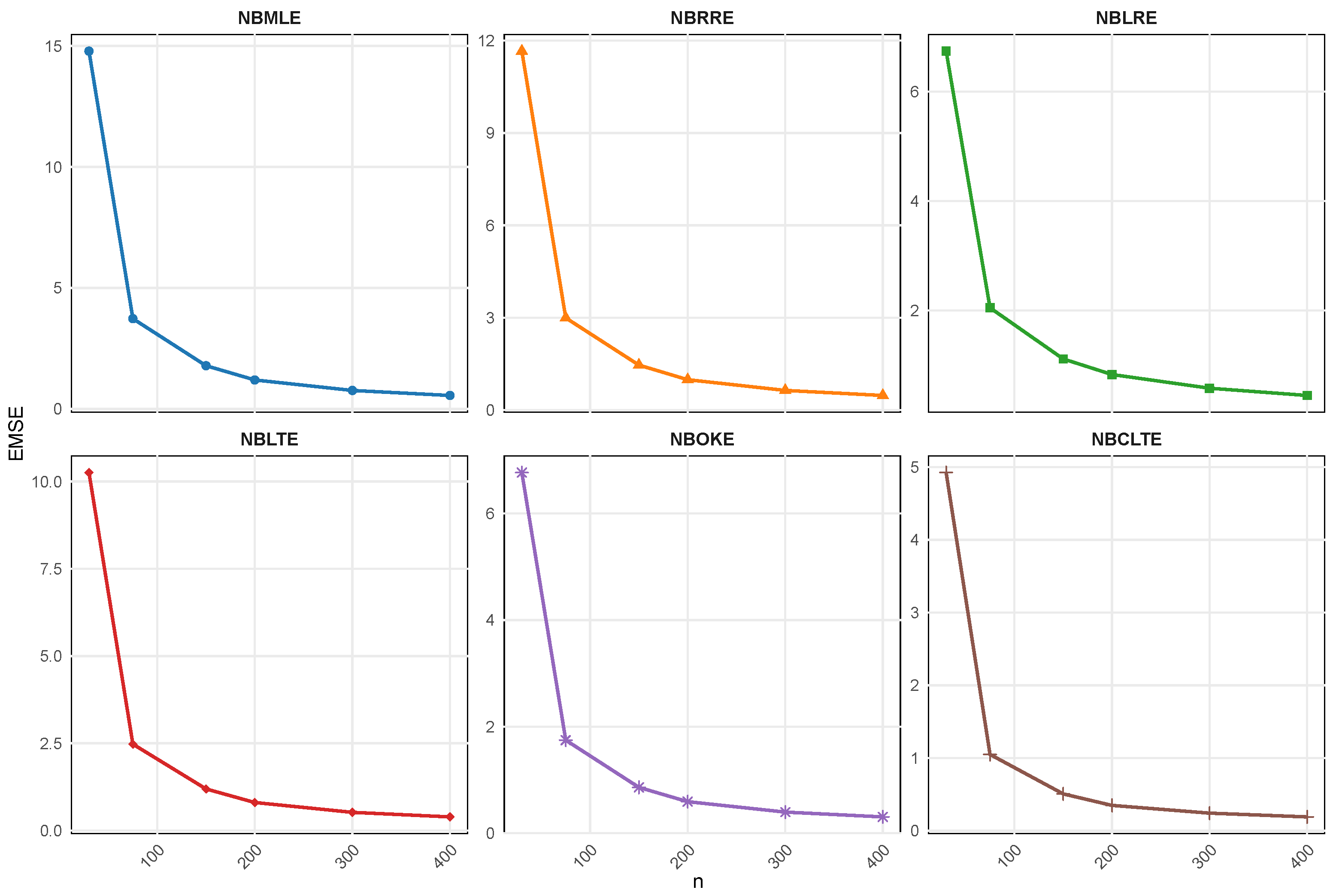
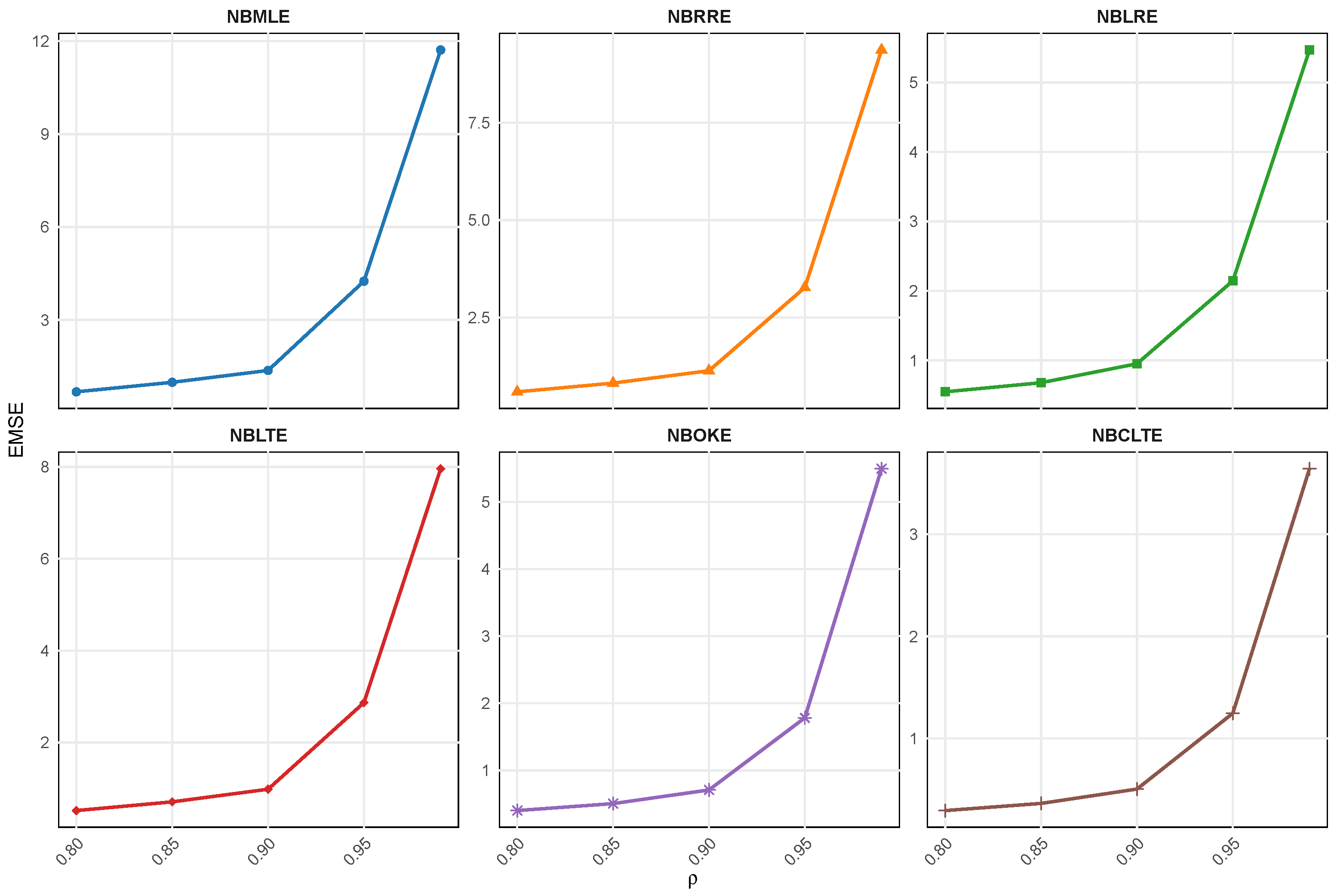
The simulation results show the performance of the proposed NBCLTE compared to five known estimators of the NBRM. Table 2, Table 3, Table 4, Table 5, Table 6 and Table 7 and Figure 1, Figure 2, Figure 3 and Figure 4 present the EMSE and EMAE of the NBMLE, NBRRE, NBLRE, NBLTE, NBOKE, and NBCLTE for various combinations of the parameters n, p, $\vartheta$, and $\rho$.

Table 2. EMSE and EMAE values for different estimators in the NBRM when p = 3 and $\vartheta$ = 1.

		EMSE						EMAE
$\mathit{\rho }$	$\mathit{n}$	NBMLE	NBRRE	NBLRE	NBLTE	NBOKE	NBCLTE	NBMLE	NBRRE	NBLRE	NBLTE	NBOKE	NBCLTE
		-	$\widehat{\mathit{k}}$	$\widehat{\mathit{d}}$	$\widehat{\mathit{k}}$ ,  $\widehat{\mathit{d}}$	$\widehat{\mathit{k}}$ ,  $\widehat{\mathit{d}}$	$\widehat{\mathit{f}\left(\mathit{k}\right)}$	-	$\widehat{\mathit{k}}$	$\widehat{\mathit{d}}$	$\widehat{\mathit{k}}$ ,  $\widehat{\mathit{d}}$	$\widehat{\mathit{k}}$ ,  $\widehat{\mathit{d}}$	$\widehat{\mathit{f}\left(\mathit{k}\right)}$
0.80	30	1.21588	0.91920	0.94930	0.76010	0.48219	0.29219	1.69001	1.45378	1.49972	1.30563	1.03846	0.75331
	75	0.33207	0.28718	0.30630	0.26351	0.19563	0.14439	0.90356	0.83963	0.86753	0.80955	0.69338	0.59870
	150	0.15266	0.14075	0.14748	0.13683	0.11226	0.10152	0.60973	0.58613	0.59939	0.57958	0.52572	0.50240
	200	0.10836	0.10161	0.10540	0.10001	0.08462	0.07979	0.51119	0.49535	0.50406	0.49234	0.45325	0.44090
	300	0.07467	0.07105	0.07336	0.07033	0.06155	0.05957	0.42558	0.41566	0.42182	0.41403	0.38847	0.38252
	400	0.05481	0.05290	0.05415	0.05264	0.04768	0.04695	0.36478	0.35853	0.36247	0.35781	0.34095	0.33813
0.85	30	1.19866	0.91999	0.94563	0.78560	0.50833	0.34334	1.64936	1.42839	1.47285	1.29944	1.04456	0.81758
	75	0.47945	0.39761	0.43004	0.34710	0.24446	0.16089	1.06329	0.96456	1.00666	0.90536	0.75473	0.60405
	150	0.18994	0.17104	0.18097	0.16367	0.12831	0.11000	0.66790	0.63415	0.65196	0.62333	0.55120	0.51357
	200	0.14440	0.13151	0.13866	0.12762	0.10120	0.09050	0.58381	0.55766	0.57193	0.55104	0.49135	0.46614
	300	0.08587	0.08101	0.08407	0.08004	0.06831	0.06579	0.45015	0.43763	0.44527	0.43554	0.40352	0.39590
	400	0.06402	0.06116	0.06302	0.06069	0.05349	0.05223	0.39028	0.38190	0.38714	0.38072	0.35863	0.35428
0.90	30	2.74639	1.81368	1.71278	1.59333	0.81229	0.62358	2.36930	1.85637	1.88383	1.67678	1.20362	1.00189
	75	0.75147	0.57374	0.62530	0.46476	0.29312	0.15700	1.30913	1.13237	1.19312	1.01520	0.79996	0.53032
	150	0.27849	0.24037	0.25861	0.22186	0.16100	0.12038	0.80925	0.75227	0.77986	0.72796	0.61948	0.54165
	200	0.18376	0.16424	0.17527	0.15644	0.11939	0.10166	0.65075	0.61589	0.63538	0.60426	0.52889	0.49072
	300	0.11450	0.10591	0.11107	0.10383	0.08443	0.07909	0.52042	0.50120	0.51245	0.49721	0.45010	0.43586
	400	0.09668	0.09019	0.09422	0.08878	0.07365	0.06993	0.47488	0.45922	0.46867	0.45639	0.41710	0.40658
0.95	30	3.11513	2.14694	2.00343	1.83456	0.95169	0.67472	2.59959	2.07195	2.07805	1.84264	1.31705	1.02195
	75	1.10198	0.81066	0.87133	0.64757	0.39064	0.22183	1.56473	1.31572	1.38479	1.15240	0.89121	0.59259
	150	0.49351	0.38919	0.42809	0.32773	0.21172	0.11723	1.05642	0.93309	0.98351	0.86219	0.68529	0.48637
	200	0.42605	0.34977	0.38630	0.30249	0.20256	0.12626	0.96963	0.87499	0.92234	0.82021	0.66618	0.51616
	300	0.26150	0.22568	0.24553	0.20795	0.14826	0.11318	0.76124	0.70670	0.73694	0.68370	0.57575	0.50561
	400	0.16803	0.14952	0.16064	0.14291	0.10668	0.09187	0.61427	0.57989	0.60032	0.56961	0.49315	0.45946
0.99	30	22.76233	13.89376	9.83011	12.64932	5.39419	3.95505	6.80020	4.88595	4.34744	4.55536	2.72464	2.16447
	75	5.12777	3.15156	2.69971	2.71296	1.19288	0.75839	3.27984	2.40860	2.33443	2.14210	1.35766	0.95357
	150	2.60623	1.70276	1.73734	1.38423	0.63704	0.41806	2.31652	1.78133	1.86288	1.53167	1.01622	0.72575
	200	1.68368	1.09996	1.20497	0.84661	0.38374	0.23411	1.87989	1.46504	1.57509	1.22803	0.82554	0.56401
	300	1.29189	0.89730	0.99243	0.70054	0.35255	0.21311	1.62314	1.30997	1.40701	1.11828	0.79014	0.51746
	400	0.86487	0.63135	0.71322	0.49330	0.27436	0.14645	1.33466	1.11565	1.20456	0.97045	0.71273	0.40361

Table 3. EMSE and EMAE values for different estimators in the NBRM when p = 3 and $\vartheta$ = 2.

		EMSE						EMAE
$\mathit{\rho }$	$\mathit{n}$	NBMLE	NBRRE	NBLRE	NBLTE	NBOKE	NBCLTE	NBMLE	NBRRE	NBLRE	NBLTE	NBOKE	NBCLTE
		-	$\widehat{\mathit{k}}$	$\widehat{\mathit{d}}$	$\widehat{\mathit{k}}$,  $\widehat{\mathit{d}}$	$\widehat{\mathit{k}}$ ,  $\widehat{\mathit{d}}$	$\widehat{\mathit{f}\left(\mathit{k}\right)}$	-	$\widehat{\mathit{k}}$	$\widehat{\mathit{d}}$	$\widehat{\mathit{k}}$ ,  $\widehat{\mathit{d}}$	$\widehat{\mathit{k}}$, $\widehat{\mathit{d}}$	$\widehat{\mathit{f}\left(\mathit{k}\right)}$
0.80	30	0.71421	0.56984	0.60383	0.48308	0.32797	0.20287	1.29275	1.14544	1.19007	1.05214	0.86052	0.63832
	75	0.18567	0.16745	0.17647	0.16100	0.12664	0.10955	0.67306	0.63891	0.65559	0.62878	0.55555	0.51879
	150	0.09430	0.08926	0.09230	0.08823	0.07621	0.07315	0.48042	0.46784	0.47526	0.46565	0.43359	0.42512
	200	0.06876	0.06585	0.06757	0.06546	0.05814	0.05663	0.41552	0.40697	0.41187	0.40597	0.38337	0.37841
	300	0.04831	0.04677	0.04774	0.04659	0.04255	0.04190	0.34429	0.33902	0.34226	0.33850	0.32419	0.32176
	400	0.03318	0.03242	0.03292	0.03236	0.03029	0.03008	0.28518	0.28199	0.28401	0.28176	0.27285	0.27171
0.85	30	0.65081	0.52202	0.55696	0.45068	0.31522	0.21448	1.23359	1.09927	1.14396	1.01942	0.84669	0.67527
	75	0.28002	0.24340	0.26109	0.22497	0.16564	0.13034	0.80292	0.74792	0.77483	0.72357	0.61946	0.54882
	150	0.11233	0.10475	0.10899	0.10290	0.08595	0.08041	0.52086	0.50343	0.51298	0.50004	0.45801	0.44436
	200	0.10134	0.09494	0.09866	0.09354	0.07871	0.07450	0.49493	0.47972	0.48844	0.47696	0.43887	0.42795
	300	0.05377	0.05180	0.05306	0.05154	0.04641	0.04559	0.35953	0.35322	0.35713	0.35252	0.33538	0.33229
	400	0.03944	0.03829	0.03904	0.03817	0.03510	0.03467	0.31175	0.30739	0.31013	0.30701	0.29502	0.29317
0.90	30	1.78766	1.16641	1.20143	0.98353	0.50371	0.35441	1.94902	1.53671	1.60307	1.36677	0.99454	0.80161
	75	0.49815	0.41042	0.44545	0.35850	0.24594	0.16015	1.06098	0.95852	1.00259	0.90042	0.73768	0.57718
	150	0.15091	0.13587	0.14366	0.13146	0.10176	0.08869	0.59756	0.56743	0.58290	0.56000	0.49272	0.46176
	200	0.11483	0.10649	0.11153	0.10426	0.08561	0.07997	0.52184	0.50310	0.51422	0.49897	0.45315	0.43887
	300	0.07175	0.06827	0.07047	0.06770	0.05897	0.05732	0.41287	0.40308	0.40905	0.40173	0.37589	0.37046
	400	0.06098	0.05829	0.05999	0.05792	0.05109	0.04980	0.38085	0.37267	0.37769	0.37173	0.34987	0.34547
0.95	30	1.95106	1.35103	1.33637	1.11167	0.61250	0.39727	2.04114	1.64535	1.68746	1.43498	1.06250	0.76192
	75	0.68117	0.52999	0.57627	0.43932	0.28080	0.15760	1.22990	1.07368	1.12869	0.97770	0.77482	0.53119
	150	0.32463	0.27313	0.29560	0.24696	0.17261	0.11857	0.85098	0.77897	0.81177	0.74687	0.61987	0.51410
	200	0.23991	0.20547	0.22393	0.19010	0.13345	0.10097	0.73525	0.68054	0.71003	0.65920	0.55167	0.48313
	300	0.16248	0.14596	0.15586	0.14032	0.10678	0.09406	0.60473	0.57340	0.59183	0.56458	0.49304	0.46371
	400	0.09579	0.08850	0.09312	0.08692	0.07043	0.06578	0.47370	0.45602	0.46693	0.45274	0.40922	0.39579
0.99	30	15.01545	9.23075	6.58046	8.47348	3.74164	2.70233	5.46879	3.96132	3.53921	3.69252	2.24798	1.73463
	75	3.49074	2.23118	2.05784	1.88305	0.86320	0.55270	2.69306	2.04298	2.03898	1.79203	1.17989	0.84412
	150	1.56454	1.06472	1.14028	0.84133	0.42134	0.26640	1.77948	1.40740	1.50107	1.19358	0.83443	0.57885
	200	1.05452	0.73800	0.83038	0.56759	0.29907	0.16504	1.47880	1.20556	1.30249	1.02907	0.74199	0.44723
	300	0.80485	0.58745	0.65859	0.46388	0.26602	0.12593	1.30109	1.09176	1.17135	0.95948	0.71520	0.39511
	400	0.48639	0.37366	0.42514	0.30660	0.18206	0.09180	1.00659	0.87285	0.93698	0.79645	0.60443	0.39265

Table 4. EMSE and EMAE values for different estimators in the NBRM when p = 6 and $\vartheta$ = 1.

		EMSE						EMAE
$\mathit{\rho }$	$\mathit{n}$	NBMLE	NBRRE	NBLRE	NBLTE	NBOKE	NBCLTE	NBMLE	NBRRE	NBLRE	NBLTE	NBOKE	NBCLTE
		-	$\widehat{\mathit{k}}$	$\widehat{\mathit{d}}$	$\widehat{\mathit{k}}$,  $\widehat{\mathit{d}}$	$\widehat{\mathit{k}}$,  $\widehat{\mathit{d}}$	$\widehat{\mathit{f}\left(\mathit{k}\right)}$	-	$\widehat{\mathit{k}}$	$\widehat{\mathit{d}}$	$\widehat{\mathit{k}}$,  $\widehat{\mathit{d}}$	$\widehat{\mathit{k}}$, $\widehat{\mathit{d}}$	$\widehat{\mathit{f}\left(\mathit{k}\right)}$
0.80	30	2.63003	2.18652	1.96445	1.84036	1.41482	0.84668	3.30570	2.99032	2.86983	2.69926	2.36407	1.71835
	75	0.89701	0.77869	0.78254	0.67576	0.54386	0.33556	1.95859	1.81754	1.82853	1.69698	1.50573	1.17109
	150	0.36628	0.33495	0.34407	0.31844	0.26201	0.21450	1.25718	1.20145	1.21834	1.17537	1.06100	0.96578
	200	0.27161	0.25279	0.25909	0.24530	0.20676	0.18183	1.08603	1.04759	1.06068	1.03410	0.94729	0.89228
	300	0.16523	0.15740	0.16050	0.15548	0.13692	0.12911	0.84262	0.82248	0.83037	0.81821	0.76750	0.74650
	400	0.12412	0.11952	0.12147	0.11867	0.10713	0.10309	0.73116	0.71766	0.72327	0.71549	0.67994	0.66780
0.85	30	3.92006	3.03212	2.49850	2.54822	1.77365	1.12075	3.94051	3.42732	3.17472	3.07798	2.57954	1.98398
	75	1.12942	0.97428	0.96735	0.82469	0.66697	0.37574	2.17962	2.01466	2.01608	1.85581	1.64845	1.20605
	150	0.41897	0.38122	0.39099	0.36011	0.29487	0.23434	1.35035	1.28675	1.30394	1.25473	1.12875	1.01187
	200	0.32900	0.30319	0.31080	0.29130	0.24192	0.20472	1.19315	1.14513	1.15989	1.12552	1.02222	0.94575
	300	0.24709	0.23177	0.23756	0.22645	0.19321	0.17465	1.03127	0.99879	1.01100	0.98866	0.91220	0.86977
	400	0.16571	0.15799	0.16109	0.15612	0.13778	0.12994	0.85425	0.83424	0.84217	0.82994	0.77939	0.75814
0.90	30	6.37041	5.07611	3.82539	4.32008	3.07094	1.92400	5.05282	4.44973	3.93985	4.00995	3.37578	2.52031
	75	1.33415	1.13374	1.11703	0.92734	0.75272	0.37614	2.36800	2.17310	2.16718	1.96502	1.75228	1.18819
	150	0.66441	0.58771	0.59949	0.52790	0.42293	0.27873	1.68690	1.58329	1.60131	1.50753	1.33736	1.09172
	200	0.53504	0.47952	0.49185	0.44192	0.35629	0.25868	1.50529	1.42352	1.44304	1.37251	1.22464	1.05078
	300	0.33781	0.30943	0.31824	0.29625	0.24243	0.20182	1.19740	1.14586	1.16209	1.12418	1.01442	0.93081
	400	0.25677	0.23966	0.24591	0.23311	0.19719	0.17510	1.04006	1.00465	1.01758	0.99274	0.91118	0.86215
0.95	30	16.51785	12.73662	7.28520	10.86071	7.29296	4.40318	8.04377	6.89851	5.29436	6.19966	4.99589	3.55969
	75	2.45678	2.00045	1.80725	1.58284	1.21770	0.59402	3.19659	2.85800	2.73855	2.50289	2.18634	1.38222
	150	1.29579	1.07496	1.04638	0.86028	0.67300	0.28919	2.32686	2.10642	2.08961	1.88251	1.64515	1.00966
	200	1.01792	0.86359	0.86335	0.71304	0.56455	0.26614	2.05580	1.88611	1.89183	1.72238	1.51398	1.02525
	300	0.62938	0.55394	0.56579	0.49662	0.39314	0.25265	1.62526	1.52221	1.54117	1.44970	1.27813	1.03552
	400	0.49249	0.44333	0.45487	0.41198	0.33149	0.24728	1.42552	1.34992	1.36901	1.30690	1.16233	1.01136
0.99	30	44.80318	35.55034	18.62933	30.78139	21.57773	14.25979	13.05713	11.35420	8.12325	10.37617	8.45602	6.43349
	75	17.93101	13.32314	7.21648	10.90893	7.09275	3.75270	8.39360	7.07233	5.22704	6.25824	4.95227	3.33644
	150	6.53238	5.00505	3.58273	3.92526	2.73519	1.26162	5.07115	4.34780	3.71211	3.74294	3.08327	1.84272
	200	5.33522	4.10967	3.05546	3.21803	2.26863	1.02447	4.61203	3.97504	3.46336	3.41858	2.84665	1.68073
	300	3.46068	2.68770	2.24058	2.03878	1.47898	0.62555	3.70552	3.21581	2.96542	2.72710	2.31652	1.31487
	400	2.35312	1.87770	1.70066	1.41669	1.08477	0.42459	3.04306	2.68303	2.57371	2.28936	1.98500	1.03231

Table 5. EMSE and EMAE values for different estimators in the NBRM when p = 6 and $\vartheta$ = 2.

		EMSE						EMAE
$\mathit{\rho }$	$\mathit{n}$	NBMLE	NBRRE	NBLRE	NBLTE	NBOKE	NBCLTE	NBMLE	NBRRE	NBLRE	NBLTE	NBOKE	NBCLTE
		-	$\widehat{\mathit{k}}$	$\widehat{\mathit{d}}$	$\widehat{\mathit{k}}$, $\widehat{\mathit{d}}$	$\widehat{\mathit{k}}$, $\widehat{\mathit{d}}$	$\widehat{\mathit{f}\left(\mathit{k}\right)}$	-	$\widehat{\mathit{k}}$	$\widehat{\mathit{d}}$	$\widehat{\mathit{k}}$, $\widehat{\mathit{d}}$	$\widehat{\mathit{k}}$, $\widehat{\mathit{d}}$	$\widehat{\mathit{f}\left(\mathit{k}\right)}$
0.80	30	1.49956	1.26104	1.21541	1.06071	0.83118	0.48070	2.50486	2.28825	2.26254	2.08856	1.84028	1.34205
	75	0.53969	0.48194	0.49247	0.44240	0.36000	0.26235	1.52336	1.43799	1.45535	1.38273	1.23919	1.06262
	150	0.22871	0.21484	0.22005	0.21030	0.18025	0.16394	0.99782	0.96710	0.97862	0.95809	0.88588	0.84690
	200	0.17817	0.16972	0.17317	0.16754	0.14770	0.13886	0.88309	0.86189	0.87040	0.85702	0.80413	0.78093
	300	0.10648	0.10316	0.10461	0.10264	0.09406	0.09134	0.68306	0.67239	0.67693	0.67093	0.64227	0.63335
	400	0.07567	0.07387	0.07469	0.07367	0.06885	0.06758	0.57586	0.56907	0.57208	0.56841	0.54962	0.54473
0.85	30	2.41819	1.83938	1.60237	1.50720	1.05737	0.61785	3.11754	2.70107	2.57408	2.40685	2.02742	1.50029
	75	0.69913	0.62149	0.63038	0.56189	0.45563	0.31512	1.73152	1.62817	1.64410	1.55347	1.38439	1.14889
	150	0.26915	0.25221	0.25799	0.24587	0.21011	0.18846	1.08302	1.04841	1.06027	1.03684	0.95696	0.90937
	200	0.20060	0.18963	0.19378	0.18640	0.16166	0.14944	0.92882	0.90351	0.91303	0.89702	0.83541	0.80573
	300	0.15443	0.14782	0.15061	0.14634	0.13024	0.12401	0.82018	0.80264	0.80993	0.79917	0.75409	0.73686
	400	0.09454	0.09165	0.09292	0.09124	0.08370	0.08145	0.64750	0.63766	0.64186	0.63644	0.60984	0.60194
0.90	30	3.66020	2.91621	2.47885	2.41069	1.76052	1.04487	3.84261	3.38313	3.16022	3.00444	2.56621	1.86494
	75	0.77145	0.67742	0.68826	0.59860	0.48368	0.30799	1.79389	1.67607	1.69385	1.58156	1.40560	1.11617
	150	0.38530	0.35249	0.36159	0.33618	0.27602	0.22683	1.29308	1.23599	1.25216	1.21011	1.09219	0.99447
	200	0.32267	0.29857	0.30662	0.28781	0.24007	0.20685	1.16290	1.11842	1.13358	1.10072	1.00274	0.93481
	300	0.22033	0.20732	0.21241	0.20320	0.17426	0.15944	0.96825	0.93929	0.95053	0.93113	0.86154	0.82618
	400	0.15872	0.15136	0.15448	0.14967	0.13202	0.12483	0.82479	0.80577	0.81368	0.80182	0.75349	0.73395
0.95	30	10.59322	7.94576	4.93874	6.68081	4.34274	2.53630	6.37495	5.40143	4.32135	4.81440	3.83953	2.67743
	75	1.49072	1.24781	1.20581	1.01431	0.80569	0.40052	2.48271	2.25622	2.23022	2.02710	1.78576	1.18176
	150	0.80473	0.69666	0.70638	0.60235	0.47722	0.27247	1.82592	1.69256	1.70879	1.58256	1.39044	1.04883
	200	0.63499	0.56056	0.57146	0.50581	0.40129	0.26570	1.62403	1.52304	1.54061	1.45383	1.28399	1.05187
	300	0.35248	0.32013	0.32955	0.30486	0.24531	0.19897	1.22149	1.16389	1.18102	1.13927	1.01883	0.92349
	400	0.28065	0.26032	0.26726	0.25264	0.21053	0.18446	1.08913	1.04894	1.06271	1.03525	0.94362	0.88690
0.99	30	27.51237	21.59452	12.06825	18.53346	12.90753	8.28110	10.26888	8.87630	6.65396	8.06159	6.58750	4.94556
	75	11.50274	8.65407	5.24714	7.13711	4.77559	2.65365	6.62239	5.59621	4.41048	4.94542	3.95942	2.67624
	150	3.89111	3.02375	2.48310	2.30355	1.67581	0.71901	3.94714	3.42856	3.13518	2.91814	2.47960	1.44177
	200	3.13555	2.46484	2.11250	1.88125	1.40215	0.62134	3.50095	3.05160	2.85156	2.59219	2.22223	1.29012
	300	2.05165	1.64570	1.51725	1.26226	0.96861	0.39311	2.85800	2.52915	2.44880	2.18168	1.89129	1.03732
	400	1.39678	1.14499	1.11760	0.88669	0.69303	0.24918	2.38056	2.14200	2.12606	1.88199	1.64457	0.90393

Table 6. EMSE and EMAE values for different estimators in the NBRM when p = 9 and $\vartheta$ = 1.

		EMSE						EMAE
$\mathit{\rho }$	$\mathit{n}$	NBMLE	NBRRE	NBLRE	NBLTE	NBOKE	NBCLTE	NBMLE	NBRRE	NBLRE	NBLTE	NBOKE	NBCLTE
		-	$\widehat{\mathit{k}}$	$\widehat{\mathit{d}}$	$\widehat{\mathit{k}}$, $\widehat{\mathit{d}}$	$\widehat{\mathit{k}}$, $\widehat{\mathit{d}}$	$\widehat{\mathit{f}\left(\mathit{k}\right)}$	-	$\widehat{\mathit{k}}$	$\widehat{\mathit{d}}$	$\widehat{\mathit{k}}$, $\widehat{\mathit{d}}$	$\widehat{\mathit{k}}$, $\widehat{\mathit{d}}$	$\widehat{\mathit{f}\left(\mathit{k}\right)}$
0.80	30	5.43981	4.62139	3.71600	3.94766	2.89301	2.06108	5.69171	5.22001	4.73499	4.75300	4.07756	3.31755
	75	1.77752	1.57671	1.50374	1.34172	1.06955	0.69839	3.28110	3.07889	3.01948	2.83027	2.50561	1.97465
	150	0.66201	0.61372	0.61907	0.57591	0.46678	0.39426	2.03649	1.95867	1.96871	1.90145	1.70164	1.57010
	200	0.43089	0.40490	0.41031	0.39103	0.32222	0.29643	1.64437	1.59338	1.60452	1.56837	1.41938	1.36646
	300	0.26781	0.25565	0.25911	0.25152	0.21463	0.20814	1.30157	1.27160	1.28019	1.26228	1.16485	1.14917
	400	0.21094	0.20329	0.20579	0.20122	0.17661	0.17398	1.14819	1.12724	1.13405	1.12208	1.05090	1.04437
0.85	30	9.60142	7.72119	5.09112	6.59785	4.28050	2.99849	7.43828	6.62724	5.49807	6.02053	4.88442	4.00280
	75	1.82776	1.61776	1.53848	1.36399	1.09090	0.69763	3.32381	3.11389	3.04929	2.84737	2.52402	1.95966
	150	0.81750	0.74822	0.74975	0.68445	0.54789	0.42593	2.25156	2.15149	2.15610	2.06370	1.83369	1.62555
	200	0.54459	0.50551	0.51087	0.47909	0.38633	0.33544	1.82627	1.75892	1.76940	1.71729	1.53574	1.44108
	300	0.37241	0.35089	0.35593	0.34082	0.28166	0.26336	1.52330	1.47833	1.48914	1.45901	1.32330	1.28379
	400	0.26015	0.24821	0.25162	0.24431	0.20795	0.20195	1.27440	1.24479	1.25327	1.23593	1.13934	1.12469
0.90	30	11.48996	9.54995	6.47016	8.32702	5.77434	4.38982	8.13538	7.34097	6.12752	6.73973	5.60378	4.75803
	75	2.56616	2.23635	2.02099	1.81571	1.43380	0.82436	3.96593	3.68870	3.52554	3.29883	2.91823	2.10183
	150	1.17767	1.05658	1.03918	0.91763	0.72629	0.47455	2.68317	2.53561	2.51956	2.36945	2.08636	1.68507
	200	0.82449	0.75228	0.75257	0.68577	0.54362	0.41592	2.24459	2.14192	2.14530	2.05183	1.81435	1.59759
	300	0.56179	0.52071	0.52635	0.49272	0.39518	0.34072	1.84736	1.77691	1.78754	1.73246	1.54352	1.44100
	400	0.40256	0.37817	0.38321	0.36635	0.30008	0.27833	1.57667	1.52774	1.53825	1.50585	1.35984	1.31408
0.95	30	54.60220	41.17663	22.55550	37.39081	21.28112	16.93196	16.49239	14.20974	10.58930	13.22432	10.15449	8.83453
	75	5.23686	4.47960	3.57573	3.61304	2.78029	1.67019	5.58292	5.12769	4.60841	4.52652	3.96149	2.89976
	150	2.50443	2.16324	1.95126	1.71044	1.35242	0.70554	3.88921	3.59542	3.43011	3.17271	2.79687	1.89895
	200	1.83216	1.59564	1.50624	1.27508	1.01407	0.51760	3.31143	3.08009	3.00205	2.75229	2.42939	1.67825
	300	1.00408	0.90150	0.89217	0.79424	0.61919	0.41945	2.46503	2.33152	2.32344	2.19723	1.92123	1.59277
	400	0.76528	0.69623	0.69770	0.63693	0.49763	0.38228	2.14219	2.04040	2.04486	1.95764	1.71732	1.51622
0.99	30	91.81773	80.15670	37.85913	71.77189	53.23354	42.03483	22.57904	20.87948	14.15278	19.49013	16.55927	14.12122
	75	26.94717	22.68956	11.29648	18.70539	13.50892	8.46640	12.52055	11.37479	8.00026	10.17201	8.54322	6.42068
	150	15.23318	12.54446	6.78603	9.99250	7.06364	3.94861	9.37876	8.41518	6.20682	7.36004	6.12437	4.21602
	200	8.73772	7.20605	4.64177	5.61542	3.99590	2.03413	7.19606	6.47242	5.20501	5.62063	4.69796	3.11319
	300	5.33112	4.42826	3.31430	3.31834	2.48165	1.12599	5.62306	5.08409	4.41989	4.31499	3.72111	2.27391
	400	4.13225	3.46839	2.79052	2.60104	1.99194	0.88988	4.93825	4.49189	4.04804	3.82518	3.33167	1.98844

Table 7. EMSE and EMAE values for different estimators in the NBRM when p = 9 and $\vartheta$ = 2.

		EMSE						EMAE
$\mathit{\rho }$	$\mathit{n}$	NBMLE	NBRRE	NBLRE	NBLTE	NBOKE	NBCLTE	NBMLE	NBRRE	NBLRE	NBLTE	NBOKE	NBCLTE
		-	$\widehat{\mathit{k}}$	$\widehat{\mathit{d}}$	$\widehat{\mathit{k}}$, $\widehat{\mathit{d}}$	$\widehat{\mathit{k}}$, $\widehat{\mathit{d}}$	$\widehat{\mathit{f}\left(\mathit{k}\right)}$	-	$\widehat{\mathit{k}}$	$\widehat{\mathit{d}}$	$\widehat{\mathit{k}}$, $\widehat{\mathit{d}}$	$\widehat{\mathit{k}}$, $\widehat{\mathit{d}}$	$\widehat{\mathit{f}\left(\mathit{k}\right)}$
0.80	30	3.54472	2.99025	2.55070	2.53104	1.84146	1.27625	4.56441	4.17278	3.89764	3.78683	3.24110	2.62238
	75	1.08778	0.97803	0.96815	0.86101	0.68792	0.48532	2.60489	2.46557	2.45794	2.31862	2.05582	1.72297
	150	0.37314	0.35341	0.35835	0.34436	0.28898	0.27283	1.53169	1.49015	1.50070	1.47256	1.34586	1.31086
	200	0.25595	0.24536	0.24866	0.24186	0.20925	0.20399	1.26565	1.23891	1.24724	1.23086	1.14313	1.13051
	300	0.16554	0.16058	0.16233	0.15955	0.14286	0.14207	1.02011	1.00476	1.01008	1.00183	0.94790	0.94587
	400	0.12496	0.12201	0.12312	0.12154	0.11122	0.11118	0.89033	0.87980	0.88371	0.87827	0.84017	0.84035
0.85	30	6.51557	5.01055	3.43343	4.20240	2.57675	1.72820	6.01880	5.24137	4.45359	4.69568	3.73501	3.01378
	75	1.03858	0.94062	0.93416	0.83854	0.67389	0.49273	2.52751	2.39986	2.39653	2.27113	2.01749	1.72321
	150	0.45775	0.42794	0.43336	0.41090	0.33525	0.30278	1.69510	1.63821	1.64918	1.60817	1.44744	1.38096
	200	0.30823	0.29238	0.29664	0.28628	0.24037	0.23003	1.38606	1.34981	1.35968	1.33692	1.22316	1.19904
	300	0.21241	0.20414	0.20680	0.20184	0.17565	0.17260	1.15123	1.12859	1.13581	1.12286	1.04682	1.03903
	400	0.16013	0.15532	0.15703	0.15433	0.13816	0.13740	0.99914	0.98407	0.98935	0.98124	0.92824	0.92637
0.90	30	7.20481	5.88679	4.29791	5.00714	3.42916	2.47721	6.52165	5.84005	5.06723	5.28641	4.37429	3.62651
	75	1.45529	1.29627	1.25447	1.10630	0.88274	0.56309	2.97550	2.80263	2.76690	2.59250	2.29615	1.80556
	150	0.74253	0.68582	0.68961	0.63796	0.51545	0.42254	2.14026	2.05479	2.06208	1.98707	1.77502	1.61656
	200	0.46694	0.43646	0.44224	0.41912	0.34091	0.30817	1.70263	1.64570	1.65711	1.61576	1.45305	1.38762
	300	0.32483	0.30759	0.31207	0.30071	0.25091	0.23910	1.41701	1.37885	1.38884	1.36472	1.24532	1.21848
	400	0.24160	0.23152	0.23461	0.22846	0.19699	0.19262	1.21784	1.19224	1.20003	1.18514	1.10000	1.08937
0.95	30	34.58263	25.15887	13.46730	22.66071	12.21084	9.37304	13.25790	11.17452	8.34437	10.36318	7.70037	6.63280
	75	3.20252	2.77888	2.45246	2.25179	1.77647	1.04972	4.35472	4.04147	3.81840	3.60427	3.19538	2.34481
	150	1.52886	1.35100	1.30055	1.13210	0.89298	0.53178	3.01872	2.82805	2.78280	2.59018	2.27667	1.73206
	200	1.13465	1.01211	0.99640	0.87813	0.68659	0.44862	2.59967	2.45209	2.43833	2.29235	2.01063	1.62795
	300	0.58828	0.54270	0.54756	0.51128	0.40589	0.34478	1.88307	1.80706	1.81675	1.75851	1.55827	1.44519
	400	0.45624	0.42548	0.43129	0.40880	0.32931	0.29778	1.66330	1.60564	1.61710	1.57655	1.41095	1.34731
0.99	30	47.72015	40.80833	20.55342	35.59106	25.79282	19.17111	16.37054	14.97045	10.58023	13.78527	11.57954	9.60508
	75	15.00254	12.49746	7.26682	10.22116	7.34148	4.58909	9.37359	8.45803	6.45020	7.50161	6.29201	4.69714
	150	9.16543	7.60296	4.90214	6.03154	4.31758	2.37085	7.34966	6.63492	5.35096	5.80614	4.88226	3.37940
	200	5.18818	4.34924	3.31613	3.34434	2.50451	1.24099	5.52182	5.01758	4.40364	4.32426	3.72807	2.42258
	300	3.29737	2.79986	2.38793	2.12786	1.65336	0.75161	4.39099	4.02654	3.73523	3.47410	3.04877	1.87800
	400	2.46740	2.11679	1.90695	1.62556	1.28231	0.57432	3.78708	3.48801	3.32479	3.03537	2.66847	1.63490

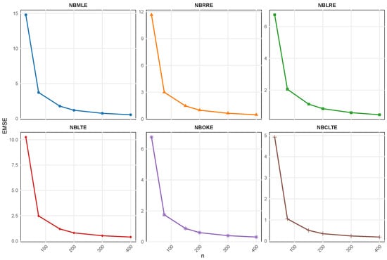
Figure 1. EMSE values for different estimators in the NBRM by sample size.

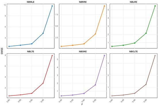
Figure 2. EMSE values for different estimators in the NBRM by multicollinearity level.

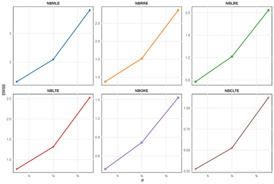
Figure 3. EMSE values for different estimators in the NBRM by the number of explanatory variables.

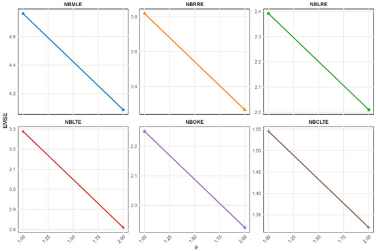
Figure 4. EMSE values for different estimators in the NBRM by dispersion parameter.

Under all the scenarios simulated, the proposed NBCLTE gives the lowest EMSE and EMAE, and the higher performance is especially noticeable for small sample sizes and severe multicollinearity. For example, when $p=3$, $\vartheta =1$, $\rho =0.99$, and $n=30$ (Table 2), the EMSE of the NBMLE is 22.762, compared to 3.955 for the NBCLTE.

The relative advantage of the NBCLTE over the other shrinkage estimators tends to get larger as the multicollinearity gets larger. For example, the difference between the NBCLTE and the next-best estimator (usually the NBOKE) is relatively small for $\rho =0.80$, but is quite large for most sample sizes at $\rho =0.99$. This seems to be the case when we consider the flexibility of the NBCLTE in the context that is most compelling for the use of biased estimators in the first place.

As one would expect, the EMSE decreases with increasing sample size for all of the estimators, as the MLE itself increases in its ability to be well-behaved asymptotically and the relative advantage of shrinkage fades. As such, the gap between NBCLTE and its competitors becomes smaller as n increases, while NBCLTE is still the best one. For example, when $p=6$, $\vartheta =2$, $\rho =0.95$ (Table 5), the EMSE gap between the NBMLE (0.281) and the NBCLTE (0.184) at $n=400$ is far smaller in relative terms than the corresponding gap at $n=30$ (10.593 vs. 2.536). That this shrinks with the sample size is as expected and as usual with shrinkage estimators, whose advantage over the NBMLE is a finite sample one.

The dispersion parameter $\vartheta$ also impacts performance: Table 2 and Table 3 show that with $\vartheta =1$ vs. $\vartheta =2$, $p=3$), the EMSE of all estimators increases with increasing response dispersion, as the variance of $\widehat{\beta }$ is inflated by higher response variability, regardless of the shrinkage mechanism applied.

As the number of predictors grows, the estimators get worse, namely, EMSE gets worse, and as the number of predictors increases, the relative gain in performance of the NBCLTE grows as seen at $p=9$ (Table 6 and Table 7) but not at $p=3$. For example, at $p=9$, $\vartheta =1$, $\rho =0.99$, $n=400$ (Table 6), the NBCLTE attains an EMSE of 0.890 versus 4.132 for the NBMLE.

The figures shown in Figure 1, Figure 2, Figure 3 and Figure 4 confirm the same patterns as Table 2, Table 3, Table 4, Table 5, Table 6 and Table 7 but are not meant to be new findings; rather, they are presented to visually show the numerical patterns at a glance over the entire range of simulation factors. It is observed from Figure 1 that all the estimators have decreasing EMSE with the increase of the sample size, and the curve of NBCLTE is the lowest. As shown in Figure 2, the difference between the NBCLTE and the competing estimators increases with the increase of the multicollinearity. As shown in Figure 3, the relative advantage of the NBCLTE increases with the number of explanatory variables. The results from this experiment can be seen in Figure 4, and it can be seen that while higher dispersion levels cause higher EMSE for all the estimators, the relative position of the estimators doesn’t change. If put together, those numbers confirm the continuity of the NBCLTE’s performance advantage on all the simulation factors included.

The rank of the four existing shrinkage estimators is more or less the same in almost all settings, with the NBOKE typically being second best after the NBLTE, followed by the NBRRE and NBLRE, and the NBMLE having the largest EMSE almost always. The ordering is consistent with the theoretical relationship between the estimators derived in Section 3 in that the two-parameter estimators (NBLTE and NBOKE) generally perform better than the single-parameter estimators (NBRRE and NBLRE) as the additional parameter gives more freedom in balancing the bias and variance. The results of the lowest EMSE and EMAE values in every simulated scenario are a direct result of the construction of the NBCLTE and not a statistical guarantee. The parameter space of the NBCLTE also includes the choices of the parameters used by each of the competing estimators as boundary points because all four of the NBRRE, NBLRE, NBLTE, and NBOKE are sub-cases of the NBCLTE (Section 3).

The simulation results indicate that the accuracy of the estimator has improved in the NBCLTE. The NBCLTE demonstrates clear progress over all estimators, particularly in challenging situations, which may be defined as cases of large multicollinearity, small sample size, or a large number of predictors. This makes the NBCLTE a good estimator for overdispersed count data.

5. Real Data Application

In order to illustrate the realism of the proposed NBCLTE estimator, we perform an application of it to a genuine data set that deals with the COVID-19 pandemic in the Kingdom of Saudi Arabia. This data set includes daily COVID-19 cases and other metrics. A data set consists of 149 observations. In this analysis, mortality represents the response variable, a count outcome that is suitable for the NBRM. The variables of the explanatory model are the confirmed cases of COVID-19 ($x_1$), recovered cases ($x_2$), active cases ($x_3$), and the calculated records ($x_4$). These variables represent various facets of the pandemic trajectory, and it is expected that these variables may be correlated, causing multicollinearity issues for the regression analysis. These predictors may be multicollinear, and this may cause the variance of the maximum likelihood estimates to be overestimated, justifying the adoption of shrinkage methods, like the proposed NBCLTE.

The descriptive statistics show strong overdispersion in the response variable, with the variance (26,194.48) much larger than the mean (41.92), corresponding to a variance-to-mean ratio of 624.88. This is confirmed by the Pearson dispersion statistic value, which is much greater than 1, the latter being the expected value under the assumption of equidispersion in the Poisson distribution, and it equals 43.80 in this instance.

To determine the best model for the COVID-19 mortality data, we ran the three models for the data, the Poisson regression model (PRM), NBRM, and the Poisson-inverse Gaussian regression model (PIGRM), and compared them with standard fit criteria. The findings show that there is a significant improvement in fit from the PRM to the overdispersed alternatives. The PRM produced a log-likelihood of −2444.649, with AIC and BIC values of 4899.298 and 4914.318, respectively. This indicates that the model was not well-suited, as it failed to satisfy the equidispersion assumption. The NBRM and the PIGRM both performed much better, however. The NBRM had a log-likelihood of −411.258, an AIC of 834.516, and a BIC of 852.540. The PIGRM had a log-likelihood of −421.844, an AIC of 855.687, and a BIC of 873.711. Both overdispersed models produce a good fit of the data structure, but the NBRM has a slightly better fit in all respects. This result supports the idea that there is notable overdispersion in the number of deaths due to COVID-19, which suggests that the negative binomial distribution should be used for further analysis.

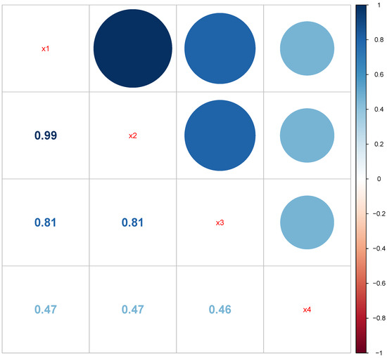
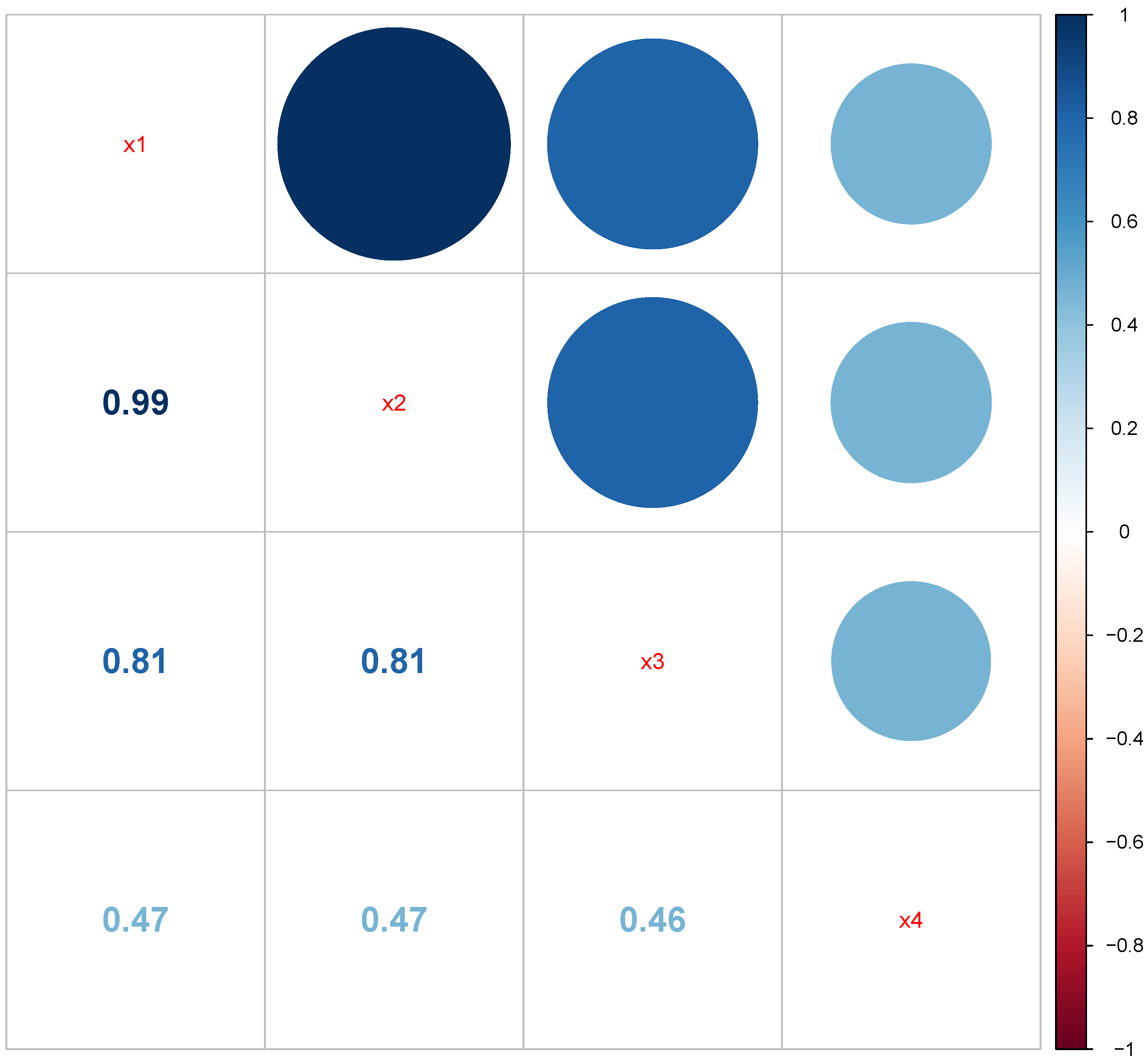
This multicollinearity of the explanatory variables was initially indicated on the correlation plot of Figure 5 and confirmed by formal diagnostic tests. The condition number (CN), calculated as the ratio of the largest eigenvalue to the smallest one, was 16,456.09, which is very high and shows that the matrix is ill-conditioned. Also, the variance inflation factors (VIFs) for the predictors were very high: 13,044.12, 12,976.75, 4.18, and 1.41, the first two being well above the recommended values. These results validate the high correlation among the predictor variables, which may result in high variances and questionable inferences in ordinary regression.

Figure 5. Correlation matrix between explanatory variables in COVID-19 mortality data.

We apply several estimators for the NBRM on the data regarding deaths due to the COVID-19 pandemic in Saudi Arabia. These provide support and insights about some of the conclusions obtained in our simulation study. Table 8 provides estimates of regression coefficients with their standard errors, 95% confidence intervals, and SMSE for each estimator.

Table 8. Parameter estimates, standard errors (in parentheses), 95% confidence intervals (in brackets), and MSE for various estimators in the NBRM applied to the COVID-19 mortality data.

Estimator	${\mathit{\beta }}_0$	${\mathit{\beta }}_1$	${\mathit{\beta }}_2$	${\mathit{\beta }}_3$	${\mathit{\beta }}_4$	SMSE
NBMLE	−0.33726	0.01347	−0.01355	−0.01248	0.01011	0.08585
	(0.29276)	(0.00249)	(0.00254)	(0.01123)	(0.00141)
	[−0.91106, 0.23654]	[0.0086, 0.01834]	[−0.01853, −0.00857]	[−0.03448, 0.00953]	[0.00735, 0.01287]
NBRRE	−0.19278	0.01334	−0.01341	−0.01301	0.00959	0.04902
	(0.16734)	(0.00248)	(0.00253)	(0.01118)	(0.00112)
	[−0.52077, 0.13521]	[0.00849, 0.01819]	[−0.01837, −0.00845]	[−0.03491, 0.0089]	[0.0074, 0.01179]
NBLRE	−0.31063	0.01345	−0.01352	−0.01257	0.01002	0.07356
	(0.26965)	(0.00248)	(0.00254)	(0.01122)	(0.00135)
	[−0.83913, 0.21787]	[0.00858, 0.01831]	[−0.0185, −0.00855]	[−0.03456, 0.00941]	[0.00737, 0.01266]
NBLTE	−0.19233	0.01334	−0.01341	−0.01301	0.00959	0.04902
	(0.16696)	(0.00248)	(0.00253)	(0.01118)	(0.00112)
	[−0.51956, 0.1349]	[0.00849, 0.01819]	[−0.01837, −0.00845]	[−0.03492, 0.0089]	[0.0074, 0.01178]
NBOKE	−0.18938	0.01172	−0.01177	−0.00789	0.00925	0.04899
	(0.16441)	(0.00218)	(0.00223)	(0.00741)	(0.00104)
	[−0.51161, 0.13285]	[0.00746, 0.01598]	[−0.01613, −0.0074]	[−0.02241, 0.00662]	[0.00721, 0.0113]
NBCLTE	−0.12641	0.01328	−0.01335	−0.01325	0.00936	0.01828
	(0.10974)	(0.00247)	(0.00253)	(0.01116)	(0.00102)
	[−0.3415, 0.08867]	[0.00843, 0.01813]	[−0.0183, −0.0084]	[−0.03513, 0.00863]	[0.00735, 0.01136]

As one might expect based on results from our simulation study, SMSE values yield an identical ordering for these estimators, validating the internal consistency of our simulation-based approach. Specifically, we observe that the proposed NBCLTE yields the smallest SMSE value (SMSE = 0.01828), which dwarfs both the SMSE of the second-best-performing estimator, the NBOKE (SMSE = 0.04899), and that of the NBMLE (SMSE = 0.08585); indeed, it also eclipses those of the other competitors, such as the NBRRE and NBLTE, whose performances were very close to that of the NBOKE with SMSEs of 0.04902 and 0.07356, respectively. Thus, there can be no reason why the performance of the NBCLTE could fail to equate or exceed that of the best-performing of the four nested estimators under consideration, provided this latter estimator is most appropriate given the specifics of the dataset’s collinearity structure, a point formally demonstrated in Section 3 in general terms.

Estimated coefficients indicate that multicollinearity indeed leads to very unstable results when estimating ${\beta }_0$ and ${\beta }_3$ using the NBMLE method, which produces an intercept coefficient (${\beta }_0=-0.33726$, $SE=0.29276$) and active cases coefficient (${\beta }_3=-0.01248$, $SE=0.01123$). In particular, these values are associated with much greater SEs compared to those resulting from the shrinkage estimators. Interestingly, the NBCLTE model also provides similar point estimates for these two parameters (intercept: ${\beta }_0$ = −0.12641; active cases: ${\beta }_3$ = −0.01325) but much smaller standard errors, such as a near threefold decrease in the standard error for the intercept. This suggests that most of the imprecision in the NBMLE estimator comes from the inflationary effect of collinearity rather than from the absence of information regarding the baseline mortality rate.

The degree of precision afforded by the NBCLTE estimator may further be appreciated if we consider the widths of these respective estimates’ corresponding confidence intervals. In particular, the NBCLTE provides us with a 95% confidence interval for ${\beta }_0$ of $[-0.3415,0.08867]$, compared to those delivered by the NBMLE of $[-0.91106,0.23654]$. Such reductions in the widths of our confidence bounds have substantial ramifications on both the substance of our estimable parameters and the subsequent implications of such parameterization. Specifically, because the widths of the confidence interval estimates generated through the use of the NBMLE are so large, any attempt to glean meaningful information regarding the directionality or magnitudes of the estimate’s underlying distribution is rendered impossible, in stark contrast to those yielded via the NBCLTE estimator.

Notably, we observe that the direction of association (i.e., sign) of the estimated coefficients for each of our predictors was consistent across all 6 estimators; both ${\beta }_1$ (confirmed cases) and ${\beta }_4$ (recorded cases) were positively associated with mortality, while both ${\beta }_2$ (recovered cases) and ${\beta }_3$ (active cases) were negatively associated. This consistency in signs of our estimators provides analytical justification for their robustness. Specifically, as previously noted, if the primary gain from using a shrinkage estimator such as the NBCLTE over NBMLE is simply reducing SMSE at the cost of reversing or altering the directionality of some effects, then such an estimator would be largely without benefit despite improvements in precision. We observe that the use of NBCLTE did provide additional precision relative to NBMLE while retaining the sign and approximately correct magnitude for each estimated parameter. Thus, the improved bias-variance trade-off is consistent with the observed collinearity structure of this dataset rather than achieved through indiscriminant shrinkage.

These results confirm that the practical advantages observed for the NBCLTE in our simulation experiment have direct relevance in applications involving real-world data sets affected by serious multicollinearity issues. Together with our empirical analysis, we demonstrate the consistency of the rankings derived from both simulations and actual epidemiological data on which we based this comparison. We also conclude that it does deliver clear interpretive gains when used within applied research contexts characterized by high levels of collinearity among predictors, e.g., the modeling of cumulative epidemiological counts.

6. Conclusions

The NBRM provides a flexible framework for modeling count data exhibiting overdispersion. However, high correlation among predictor variables induces multicollinearity, which inflates the variance of the conventional MLE and yields unstable and difficult-to-interpret coefficient estimates. Although numerous biased estimators have been proposed to address this problem, a gap remains in the literature regarding estimators that adapt to the data’s specific collinearity structure rather than imposing a fixed shrinkage rule. This paper introduces the NBCLTE, a new class of estimators for the NBRM that addresses multicollinearity by allowing the bias-correction function to vary continuously with the shrinkage parameter. The proposed estimator achieves a favorable bias–variance trade-off, offering a substantial improvement over previously existing methods. The NBCLTE was evaluated through both theoretical and empirical analyses. The theoretical comparisons, conducted within the MMSE framework, demonstrated that the NBCLTE dominates a broad range of existing estimators, namely the NBMLE, NBRRE, NBLRE, NBLTE, and NBOKE, under the stated sufficient conditions. These theoretical findings were corroborated by an extensive Monte Carlo simulation, in which the proposed estimator consistently achieved the lowest EMSE and EMAE across all simulation settings considered. The practical relevance of the NBCLTE was further illustrated through an application to COVID-19 mortality data from Saudi Arabia, where it produced the most stable coefficient estimates, the narrowest confidence intervals, and the lowest SMSE among all estimators considered, confirming its practical applicability under real-world collinearity conditions. Despite these advantages, several limitations of the present work should be acknowledged. First, the performance of the NBCLTE is sensitive to the estimated dispersion parameter, which suggests that further studies exploring alternative specifications of k and $f\left(k\right)$ would be valuable. Second, the proposed estimator addresses multicollinearity only and does not account for outliers or influential observations; it was evaluated on a single, highly correlated dataset from the health sciences domain, and its performance under high-dimensional settings remains unexamined. Third, the current formulation is developed specifically for the standard NBRM and has not been extended to alternative count-data frameworks such as zero-inflated or hurdle models. These limitations open several promising directions for future research, including the development of a robust extension of the NBCLTE capable of simultaneously addressing multicollinearity and outliers, its evaluation on a broader range of datasets, and the investigation of its performance beyond the standard NBRM framework, including zero-inflated and hurdle regression models.

References

- Cameron, A.C.; Trivedi, P.K. Regression Analysis of Count Data; Cambridge University Press: Cambridge, UK, 2013; Volume 53. [Google Scholar]
- Hilbe, J.M. Modeling Count Data; Cambridge University Press: Cambridge, UK, 2014. [Google Scholar]
- Pittman, B.; Buta, E.; Krishnan-Sarin, S.; O’Malley, S.S.; Liss, T.; Gueorguieva, R. Models for analyzing zero-inflated and overdispersed count data: An application to cigarette and marijuana use. Nicotine Tob. Res. 2020, 22, 1390–1398. [Google Scholar] [CrossRef] [Scilit]
- Bogale, B.; Tiruneh, G.T.; Belete, N.; Hunegnaw, B.M.; Fesseha, N.; Zergaw, T.S.; Tadesse, H.; Yeshiwas, T.; Meseret, H.; Emaway, D. Risk factors associated with zero-dose and under-immunized children, and the number of vaccination doses received by children in Ethiopia: A negative binomial regression analysis. BMC Public Health 2025, 25, 1693. [Google Scholar] [CrossRef] [Scilit] [PubMed]
- Alghamdi, F.M.; Abd-Elmougod, G.A.; El-Qurashi, M.A.; Almetwally, E.M.; Gemeay, A.M.; Hammad, A.T. A Bias-Reduced Estimator for Negative Binomial Regression with an Application to CO2 Emissions Data. Chiang Mai J. Sci. 2025, 52, e2025085. [Google Scholar] [CrossRef] [Scilit]
- Pitsha, P.; Chiruka, R.T.; Marange, C.S. A Comparison of the Robust Zero-Inflated and Hurdle Models with an Application to Maternal Mortality. Math. Comput. Appl. 2025, 30, 95. [Google Scholar] [CrossRef] [Scilit]
- Rashad, N.K.; Hammood, N.M.; Algamal, Z.Y. Restricted ridge estimator in the negative binomial regression model. Math. Stat. Eng. Appl. 2022, 71, 303–311. [Google Scholar]
- AL-Salami, R.A.A.; Khedir, K.R.; Eissa, M.; Algamal, Z.Y. A new ridge-type estimator for the negative binomial regression model. In Proceedings of the AIP Conference Proceedings; AIP Publishing LLC: Melville, NY, USA, 2025; Volume 3318, p. 070001. [Google Scholar]
- Månsson, K.; Shukur, G. A Poisson ridge regression estimator. Econ. Model. 2011, 28, 1475–1481. [Google Scholar] [CrossRef] [Scilit]
- Hoerl, A.E.; Kennard, R.W. Ridge regression: Biased estimation for nonorthogonal problems. Technometrics 1970, 12, 55–67. [Google Scholar] [CrossRef]
- Alkhamisi, M.A.; Shukur, G. Developing ridge parameters for SUR model. Commun. Stat. Methods 2008, 37, 544–564. [Google Scholar] [CrossRef] [Scilit]
- Alkhamisi, M.; Khalaf, G.; Shukur, G. Some modifications for choosing ridge parameters. Commun. Stat.-Theory Methods 2006, 35, 2005–2020. [Google Scholar] [CrossRef] [Scilit]
- Kibria, B.M.G. Performance of some new ridge regression estimators. Commun. Stat.-Simul. Comput. 2003, 32, 419–435. [Google Scholar] [CrossRef] [Scilit]
- Algamal, Z.Y. A new method for choosing the biasing parameter in ridge estimator for generalized linear model. Chemom. Intell. Lab. Syst. 2018, 183, 96–101. [Google Scholar] [CrossRef] [Scilit]
- Khalaf, G.; Shukur, G. Choosing ridge parameter for regression problems. Commun. Stat.-Theory Methods 2005, 34, 1177–1182. [Google Scholar] [CrossRef] [Scilit]
- Muniz, G.; Kibria, B.M.G. On some ridge regression estimators: An empirical comparisons. Commun. Stat. Comput. 2009, 38, 621–630. [Google Scholar] [CrossRef] [Scilit]
- Kejian, L. A new class of biased estimate in linear regression. Commun. Stat.-Theory Methods 1993, 22, 393–402. [Google Scholar] [CrossRef] [Scilit]
- Liu, K. Using Liu-type estimator to combat collinearity. Commun. Stat.-Theory Methods 2003, 32, 1009–1020. [Google Scholar] [CrossRef] [Scilit]
- Özkale, M.R.; Kaciranlar, S. The restricted and unrestricted two-parameter estimators. Commun. Stat. Methods 2007, 36, 2707–2725. [Google Scholar] [CrossRef] [Scilit]
- Lukman, A.F.; Kibria, B.M.G.; Ayinde, K.; Jegede, S.L. Modified one-parameter Liu estimator for the linear regression model. Model. Simul. Eng. 2020, 2020, 9574304. [Google Scholar] [CrossRef] [Scilit]
- Dawoud, I.; Kibria, B.M.G. A new biased estimator to combat the multicollinearity of the Gaussian linear regression model. Stats 2020, 3, 526–541. [Google Scholar] [CrossRef] [Scilit]
- Lukman, A.F.; Ayinde, K.; Binuomote, S.; Clement, O.A. Modified ridge-type estimator to combat multicollinearity: Application to chemical data. J. Chemom. 2019, 33, e3125. [Google Scholar] [CrossRef] [Scilit]
- Kibria, B.M.G.; Lukman, A.F. A new ridge-type estimator for the linear regression model: Simulations and applications. Scientifica 2020, 2020, 9758378. [Google Scholar] [CrossRef] [Scilit] [PubMed]
- Shewa, G.A.; Ugwuowo, F.I. A new hybrid estimator for linear regression model analysis: Computations and simulations. Sci. Afr. 2023, 19, e01441. [Google Scholar] [CrossRef] [Scilit]
- Kurnaz, F.S.; Akay, K.U. A new Liu-type estimator. Stat. Pap. 2015, 56, 495–517. [Google Scholar]
- Ertan, E.; Akay, K.U. A new Liu-type estimator in binary logistic regression models. Commun. Stat.-Theory Methods 2022, 51, 4370–4394. [Google Scholar] [CrossRef] [Scilit]
- Ertan, E.; Akay, K.U. A new class of Poisson Ridge-type estimator. Sci. Rep. 2023, 13, 4968. [Google Scholar] [CrossRef] [Scilit] [PubMed]
- Alghamdi, F.M.; Gemeay, A.M.; Abd-Elmougod, G.A.; Abd El-Raouf, M.M.; Habineza, A.; Hammad, A.T. A new class of Poisson-inverse Gaussian Liu-type regression estimator. J. Nonlinear Math. Phys. 2025, 32, 48. [Google Scholar] [CrossRef] [Scilit]
- Almulhim, F.A.; Hammad, A.T.A.; Riad, F.H.; El-Qurashi, M.A. A New Class of Conway–Maxwell–Poisson Liu-Type Regression Estimators for Effectively Modeling Multicollinear Count Data. Mathematics 2026, 14, 2234. [Google Scholar] [CrossRef] [Scilit]
- Månsson, K. On ridge estimators for the negative binomial regression model. Econ. Model. 2012, 29, 178–184. [Google Scholar] [CrossRef] [Scilit]
- Månsson, K. Developing a Liu estimator for the negative binomial regression model: Method and application. J. Stat. Comput. Simul. 2013, 83, 1773–1780. [Google Scholar] [CrossRef] [Scilit]
- Asar, Y. Liu-type negative binomial regression: A comparison of recent estimators and applications. In Proceedings of the Trends and Perspectives in Linear Statistical Inference: Proceedings of the LINSTAT2016 Meeting Held 22–25 August 2016 in Istanbul, Turkey; Springer: Berlin/Heidelberg, Germany, 2018; pp. 23–39. [Google Scholar]
- Kandemir Çetinkaya, M.; Kaçıranlar, S. Improved two-parameter estimators for the negative binomial and Poisson regression models. J. Stat. Comput. Simul. 2019, 89, 2645–2660. [Google Scholar] [CrossRef] [Scilit]
- Jabur, D.M.; Rashad, N.K.; Algamal, Z.Y. Jackknifed Liu-type estimator in the negative binomial regression model. Int. J. Nonlinear Anal. Appl. 2022, 13, 2675–2684. [Google Scholar]
- Koç, T.; Koç, H. A New Effective Jackknifing Estimator in the Negative Binomial Regression Model. Symmetry 2023, 15, 2107. [Google Scholar] [CrossRef] [Scilit]
- Ismael, H.A.; Algamal, Z.Y. A new shrinkage estimator in negative binomial regression model. Electron. J. Appl. Stat. Anal. 2025, 18, 213–224. [Google Scholar]
- Rashad, N.K.; Hammood, N.M.; Algamal, Z.Y. Generalized ridge estimator in negative binomial regression model. In Proceedings of the Journal of Physics: Conference Series; IOP Publishing: Bristol, UK, 2021; Volume 1897, p. 012019. [Google Scholar]
- Alobaidi, N.N.; Shamany, R.E.; Algamal, Z.Y. A new ridge estimator for the negative binomial regression model. Thail. Stat. 2021, 19, 115–124. [Google Scholar]
- Farebrother, R.W. Further results on the mean square error of ridge regression. J. R. Stat. Soc. Ser. B (Methodol.) 1976, 38, 248–250. [Google Scholar] [CrossRef] [Scilit]
- Alhassan, A.J.; Ahmed, S.E.; Aydin, D.; Yilmaz, E. Penalty Strategies in Semiparametric Regression Models. Math. Comput. Appl. 2025, 30, 54. [Google Scholar] [CrossRef] [Scilit]
Disclaimer/Publisher’s Note: The statements, opinions and data contained in all publications are solely those of the individual author(s) and contributor(s) and not of MDPI and/or the editor(s). MDPI and/or the editor(s) disclaim responsibility for any injury to people or property resulting from any ideas, methods, instructions or products referred to in the content. |
© 2026 by the authors. Licensee MDPI, Basel, Switzerland. This article is an open access article distributed under the terms and conditions of the Creative Commons Attribution (CC BY) license.