Statistical Properties and Actuarial Measures of Exponentiated Type II Topp-Leone-G Family of Distributions with Insurance Applications

Abstract

In this work, a type II Topp-Leone-G family of distributions is parametrically transformed to create a new flexible family of continuous probability distributions called exponentiated type II Topp-Leone-G distribution through exponentiation. A variety of density shapes and hazard rate behaviors, such as increasing, decreasing, bathtub, inverted bathtub-shaped, and unimodal forms, can be captured by the proposed family, which generalizes several current lifetime models. In addition to discussing significant special cases that correspond to well-known distributions, explicit expressions for the cumulative distribution function, probability density function, survival function, hazard rate function, quantile function, actuarial measures, and linear representation of the probability density function are derived. The maximum likelihood approach is used for parameter estimation, and the simulation study provides a brief discussion of the estimator’s asymptotic characteristics. Kolmogorov–Smirnov and Cramer–Von Mises goodness-of-fit metrics and their p-values, along with information criteria like Akaike Information Criterion, Bayesian Information Criterion, Consistent Akaike Information Criterion, and Hannan–Quinn Information Criterion, are used to evaluate the appropriateness of the model. Furthermore, to visually assess model performance, graphical diagnostic techniques, such as density and distribution function overlays, quantile–quantile plots, and probability–probability plots, are used. Real-life datasets are analyzed to show the applicability of the exponentiated type II Topp-Leone-G family using Weibull distribution as the baseline, and its performance is compared with some other competing distributions. The findings demonstrate the potential utility of the proposed model in the areas of insurance and related applied domains by showing that it fits better than the competing models considered.

1. Introduction

A key component of contemporary actuarial science and risk management is the precise modeling of loss severity and frequency. To determine fair premiums, forecast possible liabilities, and make sure solvency capital requirements are satisfied, insurance companies rely on strong statistical distributions [1]. Classical distributions like the Weibull, Gamma, and exponential have been used extensively in the past. However, real-world insurance data frequently displays features that these conventional models are unable to sufficiently capture, such as heavy tails, high skewness, and complex forms, especially in domains like property-casualty and reinsurance [2].

This shortcoming has prompted a great deal of study into creating probability distributions that are more adaptable and broadly applicable. There are many techniques for creating new families of distributions in the literature, most of which involve enhancing the flexibility of a baseline distribution by adding one or more shape factors. The exponentiated generalized family, the T-X method, and other compounding techniques are recent examples that have effectively generated models that can fit intricate actuarial and financial datasets [3,4]. Because a better fit to the underlying loss distribution immediately results in more trustworthy risk indicators, these new families are essential. For example, some of the new families of distributions recently proposed are power Topp-Leone by [5], exponential T-X by [6], type I half-logistic exponentiated-G family by [7], inverse Lomax-G family by [8], Topp-Leone Kumaraswamy Marshall-Olkin generated family of distributions by [9], power Topp-Leone exponential negative family by [10], two-parameter family of distributions by [11], extended odd Inverse Weibull-G family of distributions by [12], truncated inverse Lomax generated family by [13], Topp-Leone exponentiated-G family by [14], Topp-Leone Kumaraswamy-G family by [15], exponentiated Pareto-G family by [16] and Topp-Leone-G family by [17], which have been developed to better fit the real-life datasets.

Quantitative risk measures are also highly valued in the regulatory environment, especially in frameworks such as Solvency II. Of these, value at risk (VaR) and tail value at risk (TVaR) are important. VaR is a quantile-based metric that estimates the maximum expected loss at a given confidence level over a certain time horizon. TVaR, sometimes referred to as conditional VaR or expected shortfall, is a more logical risk metric that captures the severity of losses in the tail of the distribution by quantifying the expected loss given that the loss surpasses the VaR threshold [18]. The distributional assumption of the underlying loss data directly affects how accurate these actuarial measures are.

The lack of a single, generally optimal model that can concurrently account for the varied and frequently severe properties of different insurance loss datasets continues to be a persistent difficulty in actuarial science, notwithstanding the recent growth of generalized distributions. Even though they are better than classical distributions, several current models still have drawbacks like:

• The incapacity to accurately model both heavy and light tails.
• Inadequate adaptability to capture the different levels of kurtosis and skewness found in claims data.
• Inadequate performance when modeling complex geometries or data with various modes.

This research is significant as both theoretical and practical actuarial situations can benefit from this research work. The suggested family of distributions enhances the current statistical literature from a theoretical standpoint by providing a more adaptable framework that may represent a variety of risk behaviors. The analytical tractability of the model is improved by the derivation of explicit actuarial metrics. Practically speaking, the findings offer actuaries and insurance professionals a different modeling tool that can enhance capital allocation, risk assessment, and premium computation. The suggested model enhances decision-making in insurance pricing, reserving, and solvency management by providing better fit and more precise tail risk measurements.

This work specifically addresses the issue that current probability distributions frequently fall short of offering sufficient and economical fit to a particular class of insurance loss data, resulting in potentially erroneous actuarial measurements and less than ideal risk management choices. In order to get beyond these constraints, this study suggests a new family of distributions that offers a more precise and trustworthy framework for computing crucial actuarial variables.

2. Materials and Methods

The reference [19] proposed a type II Topp-Leone-G (TIITLG) family of distributions with three new special models and studied some mathematical properties of the family with explicit expressions for the properties. The TIITLG family can change the baseline distribution’s shape, but it frequently has little effect on tail behavior. The baseline model is still largely responsible for the tail features. As a result, actuarial measures, like VaR and TVaR, might not be sufficiently sensitive to catastrophic events, upper-tail probability might be underestimated, and extreme losses might not be sufficiently captured.

The cumulative distribution function (CDF) and probability density function (PDF) of the TIITLG family of distributions are respectively given as:

$$G(x;\alpha ,\xi )=1-{\left[1-{[H(x;\xi )]}^2\right]}^{\alpha }$$

(1)

and

$$g(x;\alpha ,\xi )=2ah(x;\xi )H(x;\xi ){\left[1-{[H(x;\xi )]}^2\right]}^{\alpha -1}$$

(2)

where $x\ge 0$, $\alpha >0$ is the shape parameter and $\xi >0$ is the parameter vector for any baseline distribution chosen. Also, $h\left(x;\xi \right)$ is the PDF, and $H\left(x;\xi \right)$ is the CDF of the baseline distribution.

Reference [20] defined the exponentiated-G family of distributions with CDF and PDF given respectively as:

$$F(x;\theta ,\xi )={[G(x;\xi )]}^{\theta }$$

(3)

and

$$f(x;\theta ,\xi )=\theta g(x;\xi ){[G(x;\xi )]}^{\theta -1}.$$

(4)

where $G(x;\xi )$ is the CDF and $g(x;\xi )$ is the PDF of the baseline distribution of the exponentiated-G family of distributions.

The exponentiated-G family only adds one additional parameter, which restricts its ability to describe complex hazard-rate structures, heavy-tailed losses, multimodal phenomena, and highly skewed data. The distribution’s body and tail behaviors might not be simultaneously controlled by a single shape parameter.

To the best of our knowledge, however, no study has integrated the Weibull baseline distribution, the type II Topp-Leone generator, and the exponentiated construction into a unified framework.

Using the T-X methodology proposed by [21], the CDF of the exponentiated type II Topp-Leone-G (ETIITL-G) family of distributions is obtained and given as

$$F(x;\theta ,\alpha ,\xi )={\left[1-{\left[1-{[H(x;\xi )]}^2\right]}^{\alpha }\right]}^{\theta }.$$

(5)

To obtain the PDF of the ETIITL-G family of distributions, Equation (5) is differentiated with respect to x, and hence, the PDF is given as

$$f(x;\theta ,\alpha ,\xi )=2\theta \alpha h(x;\xi )H(x;\xi ){\left[1-{[H(x;\xi )]}^2\right]}^{\alpha -1}{\left[1-{\left[1-{[H(x;\xi )]}^2\right]}^{\alpha }\right]}^{\theta -1}.$$

(6)

where $0\le x\le \infty$, $\theta ,\alpha >0$ are the shape parameters for the proposed family of distributions and $\xi >0$ is the parameter vector for any baseline distribution chosen. Also, $h(x;\xi )$ is the PDF, and $H(x;\xi )$ is the CDF of the baseline distribution.

The originality of this research lies in the integration of exponentiated scheme with the TIITLG family resulting in a more flexible distributional framework capable of modeling complex data patterns that standard models fail to capture adequately. Unlike many existing generalized families that only introduce a single shape parameter, the ETIITL-G family of distributions incorporates two additional shape parameters that significantly enrich the distributional structure.

The motivation for deriving the ETIITL-G family is not simply the introduction of additional shape parameters. Rather, the proposed generator is developed to address the persistent challenge of simultaneously modeling diverse hazard rate structures and complex tail behaviors within a single tractable framework. Existing generated families often provide flexibility in either the body or the tail of the distribution but may struggle to accommodate both features simultaneously. The ETIITL-G family combines the strengths of the type II Topp-Leone and exponentiation mechanisms to produce a broader spectrum of density and hazard shapes while retaining mathematical tractability. Consequently, the family offers a unified framework for modeling reliability, survival, and actuarial datasets exhibiting heterogeneous risk patterns.

2.1. Expansion of Density

To enhance analytical flexibility, the CDF and PDF of the new family of distributions can be represented using general binomial expansion, given as

$${(1-Z)}^{\omega }={\displaystyle \sum _{j=0}^{\infty }{(-1)}^j}\left(\begin{array}{c}\omega \\ j\end{array}\right)Z^j.$$

(7)

This expansion is valid whenever $\left|Z\right|<1$ and for $Z=1$ under additional condition $\omega >0$.

Using Equation (7) on Equation (5), the CDF of ETIITL-G can be represented as

$$F(x;\theta ,\alpha ,\xi )={\displaystyle \sum _{n=0}^{\infty }{\displaystyle \sum _{k=0}^{\infty }{(-1)}^{n+k}}}\left(\begin{array}{c}\theta \\ n\end{array}\right)\left(\begin{array}{c}\alpha n\\ k\end{array}\right){[H(x;\xi )]}^{2k}.$$

(8)

Also, using Equation (7) on Equation (6), the PDF of ETIITL-G can be represented as

$$f(x;\theta ,\alpha ,\xi )=2\theta \alpha {\displaystyle \sum _{b=0}^{\infty }{\displaystyle \sum _{t=0}^{\infty }{(-1)}^{b+t}}\left(\begin{array}{c}\theta -1\\ b\end{array}\right)}\left(\begin{array}{c}\alpha (b+1)-1\\ t\end{array}\right)h(x;\xi ){[H(x;\xi )]}^{2t+1}.$$

(9)

Equations (8) and (9) are the linear forms of Equations (5) and (6) and will be used to derive some of the mathematical properties of the ETIITL-G family of distributions.

2.2. Properies of the ETIITL-G Family of Distributions

In this section, some of the properties of the ETIITL-G family of distributions, such as moments, moment generating function, Rényi entropy, reliability and hazard functions, quantile function, order statistics and actuarial measures, are described.

2.2.1. Moments

Moments of a random variable play a crucial role in statistical distribution theory. From the derived moments, other measures such as mean, skewness, kurtosis, and variance can also be derived. The rth moment of X is obtained by

$$E(X^r)={\displaystyle {\int }_{-\infty }^{\infty }{x}^r}f(x)dx.$$

(10)

The moments of the ETIITL-G family of distributions are given as

$$E(X^r)=2\theta \alpha {\displaystyle {\displaystyle \sum _{b=0}^{\infty }}{\displaystyle \sum _{t=0}^{\infty }{\left(-1\right)}^{b+t}}}\left(\begin{array}{c}\theta -1\\ b\end{array}\right)\left(\begin{array}{c}\alpha \left(b+1\right)-1\\ t\end{array}\right){\displaystyle {\int }_0^{\infty }{x}^r}h\left(x;\xi \right){\left[H\left(x;\xi \right)\right]}^{2t+1}dx$$

(11)

The rth moments for ETIITL-G exist whenever $E(X^r)<\infty$. In particular, all moments exist if the density decreases sufficiently rapidly so the integral converges for every $r>0$.

2.2.2. Moment Generating Function (mgf)

The mgf is a strong tool in probability theory used to examine random variables. It turns a random variable into a function that simplifies the calculation of crucial features such as the mean, variance, skewness, and kurtosis. The mgf $M_x(t)=E(e^{tx})$ of a random variable X is defined as:

$$M_x(t)={\displaystyle {\int }_{-\infty }^{\infty }{e}^{tx}}f(x)dx.$$

(12)

The mgf of ETIITL-G is given by

$$M_x(t)=2\theta a{\displaystyle {\displaystyle \sum _{b,t=0}^{\infty }}{\left(-1\right)}^{b+t}}\left(\begin{array}{c}\theta -1\\ b\end{array}\right)\left(\begin{array}{c}\alpha \left(b+1\right)-1\\ t\end{array}\right){\displaystyle {\int }_0^{\infty }{x}^r}h\left(x;\xi \right){\left[H\left(x;\xi \right)\right]}^{2t+1}dx.$$

(13)

The mgf exists when $M_x(t)<\infty$ holds in an open neighborhood of $t=0$. For heavy tailed distributions, the mgf may fail to exist for positive values of $t$ even when several finite moments are available.

2.2.3. Rényi Entropy

According to [22], entropy is a measure of variation or uncertainty of a random variable. Rényi entropy has diverse applications in the field of information and application theory, economics, physics and other complex schemes. The Rényi entropy of a given random variable is given as

$${\mathrm{I}}_R(\mathsf{\Psi })={\displaystyle \frac{1}{1-\mathsf{\Psi }}}\log {\displaystyle {\displaystyle \underset{0}{\overset{1}{\int }}}{[f(x)]}^{\mathsf{\Psi }}}dx,$$

(14)

where $\mathsf{\Psi }>0\mathrm{and}\mathsf{\Psi }\ne 0$.

The Rényi entropy for the ETIITL-G family of distributions is given as

$${\mathrm{I}}_R\left(\mathsf{\Psi }\right)={\displaystyle \frac{1}{1-\mathsf{\Psi }}}{\left(2\theta a{\displaystyle \sum _{b=0}^{\infty }{\displaystyle \sum _{t=0}^{\infty }{\left(-1\right)}^{b+t}}}\left(\begin{array}{c}\theta -1\\ b\end{array}\right)\left(\begin{array}{c}\alpha \left(b+1\right)-1\\ t\end{array}\right)\right)}^{\mathsf{\Psi }}\log {\displaystyle {\displaystyle \underset{0}{\overset{1}{\int }}}{\left(h\left(x;\xi \right){\left[H\left(x;\xi \right)\right]}^{2t+1}\right)}^{\mathsf{\Psi }}dx}$$

(15)

2.2.4. Survival Function (sf)

The sf represents the likelihood that a person or something will live longer than a specific amount of time. It provides a summary of the population’s survival experiences. The sf is mathematically defined as:

$$S(x)=1-F(x).$$

(16)

The sf of ETIITL-G is given as:

$$S(x)=1-{\left[1-{\left[1-{\left[H\left(x\right)\right]}^2\right]}^{\alpha }\right]}^{\theta }.$$

(17)

2.2.5. Hazard Function (hf)

The hf represents the likelihood of the event happening at a specific time, given that the person has survived up to that point. It offers insight into the probability of failure or event occurrence over time and aids in determining times of high or low risk. The mathematical representation of the hf is:

$$T(x)={\displaystyle \frac{f(x)}{S(x)}}.$$

(18)

The hf of ETIITL-G is given as:

$$T(x)={\displaystyle \frac{2\theta h\alpha \left(x\right)H\left(x\right){\left[1-{\left[H\left(x\right)\right]}^2\right]}^{\alpha -1}{\left[1-{\left[1-{\left[H\left(x\right)\right]}^2\right]}^{\alpha }\right]}^{\theta -1}}{1-{\left[1-{\left[1-{\left[H\left(x\right)\right]}^2\right]}^{\alpha }\right]}^{\theta }}}$$

(19)

2.2.6. Quantile Function (qf)

In statistical analysis, the qf of a probability distribution is essential. It is fundamental to statistical modeling and calculates the value in the cdf of a distribution inversely for a given probability. The ETIITL-G family of distributions has a qf given as follows:

$$\begin{array}{c}K(x;\xi )={\left[1-{\left[1-{[H(x;\xi )]}^2\right]}^{\alpha }\right]}^{\theta }=U\\ 1-{\left[1-{\left[H\left(x;\xi \right)\right]}^2\right]}^{\alpha }=U^{{\displaystyle \frac{1}{\theta }}}\\ {\left[1-{\left[H\left(x;\xi \right)\right]}^2\right]}^{\alpha }=1-U^{{\displaystyle \frac{1}{\theta }}}\\ 1-{\left[H\left(x;\xi \right)\right]}^2={\left[1-U^{{\displaystyle \frac{1}{\theta }}}\right]}^{{\displaystyle \frac{1}{\alpha }}}\\ {\left[H\left(x;\xi \right)\right]}^2=1-{\left[1-U^{{\displaystyle \frac{1}{\theta }}}\right]}^{{\displaystyle \frac{1}{\alpha }}}\\ H\left(x;\xi \right)={\left[1-{\left[1-U^{{\displaystyle \frac{1}{\theta }}}\right]}^{{\displaystyle \frac{1}{\alpha }}}\right]}^{{\displaystyle \frac{1}{2}}}\\ x=Q(u)=H^{-1}{\left[1-{\left[1-U^{{\displaystyle \frac{1}{\theta }}}\right]}^{{\displaystyle \frac{1}{\alpha }}}\right]}^{{\displaystyle \frac{1}{2}}}.\end{array}$$

(20)

To obtain the median of ETIITL-G, we set $U=0.5$ in Equation (20).

2.3. Order Statistics

Order statistics are used for numerous reasons, including reliability, outlier detection, quality control, disaster planning, statistical inference, health-related data analysis and goodness-of-fit assessment. Thus, the order statistic of a distribution is given as

$$f_{r:n}(x)={\displaystyle \frac{f(x)}{B(r,n-r+1)}}{\displaystyle \sum _{v=0}^{n-r}{\left(-1\right)}^v\left(\begin{array}{c}n-r\\ v\end{array}\right)}F{(x)}^{v+r-1}.$$

(21)

We substitute Equations (5) and (6) into Equation (21) to obtain the rth order statistic of the ETIITL-G family of distributions, which is given as:

$$\begin{array}{c}{f}_{r:n}(x)={\displaystyle \frac{2\theta \alpha }{B(r,n-r+1)}}{\displaystyle \sum _{b,t=0}^{\infty }{\left(-1\right)}^{b+t}}\left(\begin{array}{c}\theta -1\\ b\end{array}\right)\left(\begin{array}{c}\alpha \left(b+1\right)-1\\ t\end{array}\right)h\left(x;\xi \right){\left[H\left(x;\xi \right)\right]}^{2t+1}\\ \times {\displaystyle \sum _{v=0}^{n-r}{\left(-1\right)}^v\left(\begin{array}{c}n-r\\ v\end{array}\right)}{\left[{\displaystyle \sum _{n,k=0}^{\infty }{\left(-1\right)}^{n+k}}\left(\begin{array}{c}\theta \\ n\end{array}\right)\left(\begin{array}{c}\alpha n\\ k\end{array}\right){\left[H\left(x;\xi \right)\right]}^{2k}\right]}^{v+r-1}\end{array}$$

(22)

The PDF of the minimum order statistic of ETIITL-G is given as

$$\begin{array}{c}{f}_{1:n}(x)=2n\theta \alpha {\displaystyle \sum _{b,t=0}^{\infty }{\left(-1\right)}^{b+t}}\left(\begin{array}{c}\theta -1\\ b\end{array}\right)\left(\begin{array}{c}\alpha \left(b+1\right)-1\\ t\end{array}\right)h\left(x;\xi \right){\left[H\left(x;\xi \right)\right]}^{2t+1}\\ \times {\displaystyle \sum _{v=0}^{n-1}{\left(-1\right)}^v\left(\begin{array}{c}n-1\\ v\end{array}\right)}{\left[{\displaystyle \sum _{n,k=0}^{\infty }{\left(-1\right)}^{n+k}}\left(\begin{array}{c}\theta \\ n\end{array}\right)\left(\begin{array}{c}\alpha n\\ k\end{array}\right){\left[H\left(x;\xi \right)\right]}^{2k}\right]}^v\end{array}$$

(23)

The PDF of the maximum order statistic of ETIITL-G is given as

$$\begin{array}{c}{f}_{n:n}(x)=2n\theta \alpha {\displaystyle \sum _{b,t=0}^{\infty }{\left(-1\right)}^{b+t}}\left(\begin{array}{c}\theta -1\\ b\end{array}\right)\left(\begin{array}{c}\alpha \left(b+1\right)-1\\ t\end{array}\right)h\left(x;\xi \right){\left[H\left(x;\xi \right)\right]}^{2t+1}\\ \times {\left[{\displaystyle \sum _{n,k=0}^{\infty }{\left(-1\right)}^{n+k+v}}\left(\begin{array}{c}\theta \\ n\end{array}\right)\left(\begin{array}{c}\alpha n\\ k\end{array}\right){\left[H\left(x;\xi \right)\right]}^{2k}\right]}^{v+n-1}\end{array}$$

(24)

2.4. Actuarial Measures

This section describes the actuarial measures used to evaluate both exposure to risk and tail behavior in financial and insurance usage.

2.4.1. Value at Risk

Reference [23] described the value at risk (VaR) as the quantile of a probability model and a standard risk measure used to determine the exposure to risk. In the family case of ETIITL-G, the VaR is calculated by substituting (U) with (q) in the quantile function.

$$VaR=H^{-1}{\left[1-{\left[1-q^{{\displaystyle \frac{1}{\theta }}}\right]}^{{\displaystyle \frac{1}{\alpha }}}\right]}^{{\displaystyle \frac{1}{2}}}.$$

(25)

2.4.2. Tail Value at Risk

The tail value at risk (TVaR) as defined in [24] is the expected loss given that the loss exceeds the value at risk (VaR) level $q$. TVaR is frequently treated in the current risk management literature as the same concept as the expected shortfall (ES). The TVaR can be expressed mathematically as

$$TVaR={\displaystyle \frac{1}{1-q}}{\displaystyle {\displaystyle \underset{Va{R}_q}{\overset{\infty }{\int }}}x}f(x;\theta ,\alpha ,\xi )dx.$$

(26)

The TVaR of ETIITL-G is given as

$$TVaR={\displaystyle \frac{2\theta \alpha }{1-q}}{\displaystyle {\displaystyle \sum _{b,t=0}^{\infty }}{(-1)}^{b+t}}\left(\begin{array}{c}\theta -1\\ b\end{array}\right)\left(\begin{array}{c}\alpha \left(b+1\right)-1\\ t\end{array}\right){\displaystyle {\displaystyle \underset{Va{R}_q}{\overset{\infty }{\int }}}x}h(x;\xi ){[H(x;\xi )]}^{2t+1}dx.$$

(27)

2.4.3. Tail Variance

Tail variance (TV), which was first proposed by [25], is the measure of the variation in the losses that fall outside the value at risk (VaR) threshold. A big TV implies a high degree of uncertainty and extreme losses. The ETIITL-G family TV is provided as:

$$TV={\displaystyle \frac{1}{1-q}}{\displaystyle {\displaystyle \underset{Va{R}_q}{\overset{\infty }{\int }}}{x}^2}f(x)dx-{(TVaR)}^2$$

(28)

$$TV={\displaystyle \frac{2\theta \alpha }{1-q}}{\displaystyle {\displaystyle \sum _{b,t=0}^{\infty }}{(-1)}^{b+t}}\left(\begin{array}{c}\theta -1\\ b\end{array}\right)\left(\begin{array}{c}\alpha (b+1)-1\\ t\end{array}\right){\displaystyle {\displaystyle \underset{Va{R}_q}{\overset{\infty }{\int }}}{x}^2}h(x;\xi ){[H(x;\xi )]}^{2t+1}dx-{(TVaR)}^2$$

(29)

2.4.4. Tail Variance Premium

Reference [26] established the tail variance premium (TVP), which is the cost of insurance against extreme risks and explains the cost depending on both the variability and the severity of the risk. Additionally, tail risk is typically captured in insurance pricing. The TVP of the ETIITL-G family is provided by:

$$TVP=TVaR+\lambda TV,$$

(30)

where $0<\lambda <1$.

2.5. Maximum Likelihood Estimation

In this subsection, the unknown parameters of the ETIITL-G family of distributions are estimated using the method of maximum likelihood estimation (mle). Given a random sample of size n, denoted by $x_1,x_2,\dots ,x_n$, where each observation is independently and identically distributed with the ETIITL-G, then the log-likelihood of the ETIITL-G family of distributions is given as:

$$\begin{array}{c}\log (Z)=n\log (2)+n\log (\theta )+n\log (\alpha ){\displaystyle {\displaystyle \sum _{i=1}^n}\log [h(x_i;\xi )]}+{\displaystyle {\displaystyle \sum _{i=1}^n}\log [H(x_i;\xi )]}\\ \times (\alpha -1){\displaystyle {\displaystyle \sum _{i=1}^n}\log \left[1-{[H(x_i;\xi )]}^2\right]}(\theta -1){\displaystyle {\displaystyle \sum _{i=1}^n}\log \left[1-{\left[1-{[H(x_i;\xi )]}^2\right]}^{\alpha }\right]}\end{array}$$

(31)

where $Z$ is the likelihood function of the ETIITL-G. The components of score vector $Z={(Z_{\theta },Z_{\theta },Z_{\xi })}^T$ are given as

$$Z_{\theta }={\displaystyle \frac{n}{\theta }}+{\displaystyle \sum _{i=1}^n\log \left[1-{\left[1-{[H(x_i;\xi )]}^2\right]}^{\alpha }\right]}$$

(32)

$$\begin{array}{l}{Z}_{\alpha }={\displaystyle \frac{n}{\alpha }}+{\displaystyle {\displaystyle \sum _{i=1}^n}\log \left[1-{[H(x_i;\xi )]}^2\right]}(\theta -1){\displaystyle {\displaystyle \sum _{i=1}^n}\frac{{\left[1-{[H(x_i;\xi )]}^2\right]}^{\alpha }\log \left[1-{[H(x_i;\xi )]}^2\right]}{\left[1-{\left[1-{[H(x_i;\xi )]}^2\right]}^{\alpha }\right]},}\end{array}$$

(33)

$$\begin{array}{c}{Z}_H={\displaystyle {\displaystyle \sum _{i=1}^n}\left[\frac{h{(x_i;\xi )}^{\xi }}{h(x_i;\xi )}\right]+}{\displaystyle {\displaystyle \sum _{i=1}^n}\left[\frac{H{(x_i;\xi )}^{\xi }}{H(x_i;\xi )}\right]}2(\alpha -1){\displaystyle {\displaystyle \sum _{i=1}^n}\left[\frac{H(x_i;\xi )H{(x_i;\xi )}^{\xi }}{\left[1-{[H(x_i;\xi )]}^2\right]}\right]}\\ \times (\theta -1){\displaystyle \sum _{i=1}^n\left[\frac{\alpha {\left[1-{[H(x_i;\xi )]}^2\right]}^{\alpha -1}2H(x_i;\xi )H{(x_i;\xi )}^{\xi }}{\left[1-{\left[1-{[H(x_i;\xi )]}^2\right]}^{\alpha }\right]}\right].}\end{array}$$

(34)

The mles are obtained by setting $Z_{\theta },Z_{\alpha },Z_{\xi }$ to zero and solving these equations simultaneously.

R version 4.5.2 [27] will be used to solve the equations numerically using an iterative method because they are nonlinear. The log-likelihood function lacks closed-form solutions and has a nonlinear structure. To ensure stable convergence, initial parameter values were selected, and specifically, the starting values were chosen as 1 for all the parameters. To assess robustness, several alternative starting values were also considered, and the optimization consistently converged to the same solution, indicating numerical stability of the estimation procedure. To guarantee a valid probability distribution and ensure identifiability of the model, all parameters were constrained to be strictly positive as $\kappa ,\alpha ,\theta ,\phi >0$.

The parameters are estimated using numerical optimization. The BFGS algorithm’s R implementation is used to increase convergence stability and impose parameter constraints. Convergence was assessed using gradient norms and Hessian diagnostics, and several beginning values are considered to lessen the likelihood of local maxima. If the Hessian is singular or the method does not converge, go from a gradient-based technique (BFGS) to a derivative-free approach (Nelder–Mead).

Convergence was declared when the relative change in the log-likelihood function and parameter estimates between successive iterations was less than 10⁻⁸. The default convergence tolerance of the R optimization routine was supplemented by monitoring the gradient norm to ensure that a stationary point had been reached. A maximum of 10,000 iterations was allowed for each optimization run. In all analyses reported in this study, convergence was achieved well before reaching the maximum iteration limit.

Following convergence, the observed Hessian matrix was computed numerically at the MLEs.

To address potential non-convergence issues, the optimization was repeated using multiple sets of initial values. If convergence was not achieved, the parameter estimates from the best likelihood value obtained were used as new starting values, and the optimization was restarted. Solutions associated with singular Hessian matrices, boundary estimates, or non-finite likelihood values were discarded. For all datasets analyzed in this study, the algorithm converged successfully and produced a positive-definite Hessian matrix, indicating reliable estimation results.

2.6. Submodels of the ETIITL-G Family of Distributions

In this section, we provide two baseline distributions: Weibull and inverse Weibull distributions. This is to test the flexibility and robustness of the new family of distributions in fitting complex datasets.

2.6.1. Exponentiated Type II Topp-Leone-Weibull (ETIITLW) Distribution

The Weibull distribution proposed by [28] is one of the popular distributions used in survival and reliability analysis. The CDF and PDF of the Weibull distribution with parameters $\kappa$ and $\phi$ as our baseline distribution are given by

$$H(x;\kappa ,\phi )=1-e^{-\kappa x^{\phi }},x>0,\kappa ,\phi >0.$$

(35)

$$h(x;\kappa ,\phi )=\kappa \phi x^{\phi -1}{e}^{-\kappa x^{\phi }},x>0,\kappa ,\phi >0.$$

(36)

Then, the CDF of the ETIITLW distribution is obtained by inserting Equation (35) into Equation (5) as:

$$F(x;\kappa ,\alpha ,\theta ,\phi )={\left[1-{\left[1-{\left[1-e^{-\kappa x^{\phi }}\right]}^2\right]}^{\alpha }\right]}^{\theta },$$

(37)

and the PDF of the ETIITLW distribution is obtained by differentiating Equation (37) with respect to x as:

$$f(x;\kappa ,\alpha ,\theta ,\phi )=2\theta \alpha \kappa \phi x^{\phi -1}{e}^{-\kappa x^{\phi }}{\left[1-{\left[1-e^{-\kappa x^{\phi }}\right]}^2\right]}^{\alpha -1}\left[1-e^{-\kappa x^{\phi }}\right]{\left[1-{\left[1-{\left[1-e^{-\kappa x^{\phi }}\right]}^2\right]}^{\alpha }\right]}^{\theta -1}.$$

(38)

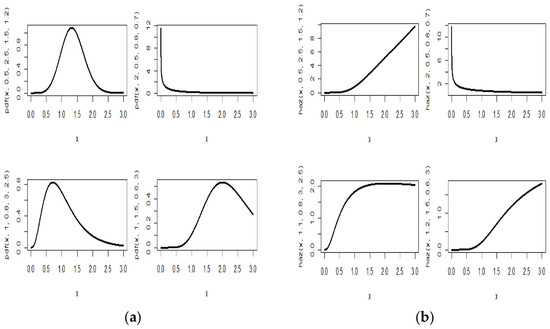
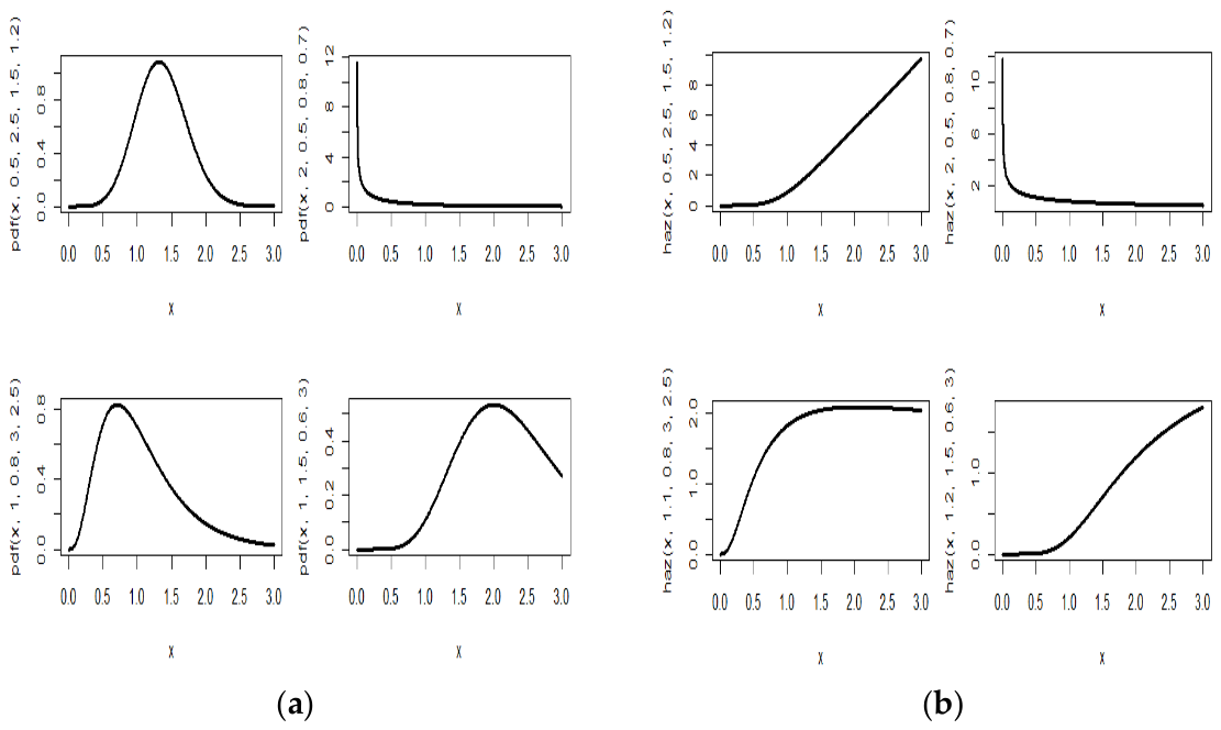
The pdf of the ETIITLW distribution for various parameter combinations is shown in Figure 1a. In showing a range of distributional shapes, the figure shows how flexible the model is. The structure of the curves can be symmetric for $\left(\kappa =0.5,\phi =2.5,\alpha =1.5,\theta =1.2\right)$, L-shape for $\left(\kappa =2.0,\phi =0.5,\alpha =0.8,\theta =0.7\right)$, positively skewed for $\left(\kappa =1.1,\phi =0.8,\alpha =3.0,\theta =2.5\right)$ and negatively skewed for $\left(\kappa =1.2,\phi =1.5,\alpha =0.6,\theta =3.0\right)$. The graphs show that different levels of variability and tail risk can be represented by symmetric, moderately skewed, and substantially right-skewed density functions produced by the ETIITLW distribution. From an actuarial point of view, the heavier-tailed configurations suggest a higher likelihood of extreme losses, which raises estimates of VaR, TVaR, TV, and TVP and, as a result, increases premiums, reserves, and solvency capital requirements. The model’s applicability for capital management, risk assessment, and claim severity modeling is improved by its capacity to handle such varied distributional behaviors within a unified framework.

Figure 1. (a) PDF of the ETIITLW distribution for selected values of the parameters illustrating the flexibility of the model in capturing different degrees of skewness, tail behavior, and peak sharpness; (b) hazard function of the ETIITLW distribution for selected values of the parameters illustrating its ability to capture increasing, decreasing, bathtub and inverted bathtub hazard behavior under different parameter settings.

Figure 1b illustrates a number of hazard functions that are essential to reliability engineering and survival analysis. The hazard functions in this plot can be increasing for $\left(\kappa =0.5,\phi =2.5,\alpha =1.5,\theta =1.2\right)$, decreasing for $\left(\kappa =2.0,\phi =0.5,\alpha =0.8,\theta =0.7\right)$, bathtub for $\left(\kappa =1.1,\phi =0.8,\alpha =3.0,\theta =2.5\right)$ and inverted bathtub hazard shapes for $\left(\kappa =1.2,\phi =1.5,\alpha =0.6,\theta =3.0\right)$. The graphs demonstrate that increasing, decreasing, bathtub and inverted bathtub hazard rate structures can be modeled using the ETIITLW distribution. The various risk mechanisms found in actuarial science and reliability engineering, such as aging effects, early-life failures, and long-term stable risk exposure, are reflected in these hazard behaviors. From an actuarial standpoint, rising hazards indicate rising claim occurrence risk and, as a result, increased premiums, reserves, and solvency capital requirements; on the other hand, falling hazards indicate early exposure risk concentration. The model’s capacity to account for various temporal risk patterns that are pertinent to choices about pricing, reserving, and capital management is what gives the figure its practical value.

Reliability Function

The reliability function of the ETIITLW distribution is given as

$$R(x)=1-{\left[1-{\left[1-{\left[1-e^{-\kappa x^{\phi }}\right]}^2\right]}^{\alpha }\right]}^{\theta }.$$

(39)

Hazard Function

The hazard function of the ETIITLW distribution is given as

$$T(x)=2\theta \alpha \kappa \phi x^{\phi -1}{e}^{-\kappa x^{\phi }}\left[B\right]{\left[1-{\left[1-{\left[B\right]}^2\right]}^{\alpha }\right]}^{\theta -1}{\left[1-{\left[B\right]}^2\right]}^{\alpha -1}{\left\{1-{\left[1-{\left[1-{\left[B\right]}^2\right]}^{\alpha }\right]}^{\theta }\right\}}^{-1},$$

(40)

where $B=1-e^{-\kappa x^{\phi }}$.

Quantile Function

The quantile function of the ETIITLW distribution is given as

$$x=Q\left(u\right)={\left[{\displaystyle \frac{-\log \left[1-{\left[1-{\left[1-u^{\frac{1}{\theta }}\right]}^{\frac{1}{\alpha }}\right]}^{\frac{1}{2}}\right]}{\kappa }}\right]}^{{\displaystyle \frac{1}{\phi }}}.$$

(41)

2.6.2. Exponentiated Type II Topp-Leone-Inverse Weibull (ETIITLIW) Distribution

The inverse Weibull (IW) distribution, another name for the Fréchet distribution, is a particular instance of the generalized extreme value distribution. The distribution of a sample of random variables’ maximum (or minimum) is modeled using this technique. This distribution is especially helpful in disciplines like reliability engineering, economics, and hydrology. According to [29], it is an appropriate model to explain mechanical component deterioration processes.

Reference [30] asserts that the IW distribution fits a number of datasets well, including the durations of an insulating fluid under the influence of a continuous stress. The CDF and PDF of the IW distribution are given as follows:

$$H\left(x;\eta ,\beta \right)=e^{-\eta x^{-\beta }},x>0,\eta ,\beta >0.$$

(42)

$$h\left(x;\eta ,\beta \right)=\eta \beta x^{-\beta -1}{e}^{-\eta x^{-\beta }},x>0,\eta ,\beta >0.$$

(43)

Then, the CDF of the ETIITLIW distribution is obtained by inserting Equation (42) into Equation (5) as:

$$F(x)={\left[1-{\left[1-e^{-2\eta x^{-\beta }}\right]}^{\alpha }\right]}^{\theta }$$

(44)

and the PDF of the ETIITLIW distribution is obtained by differentiating Equation (44) with respect to x as

$$f(x;\theta ,\alpha ,\eta ,\beta )=2\theta \alpha \eta \beta x^{-\beta -1}{\left[1-e^{-2\eta x^{-\beta }}\right]}^{\alpha -1}{e}^{-2\eta x^{-\beta }}{\left[1-{\left[1-e^{-2\eta x^{-\beta }}\right]}^{\alpha }\right]}^{\theta -1}.$$

(45)

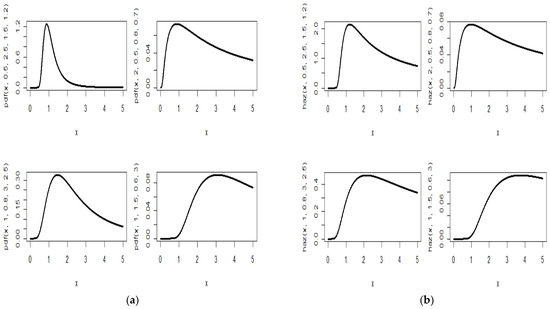
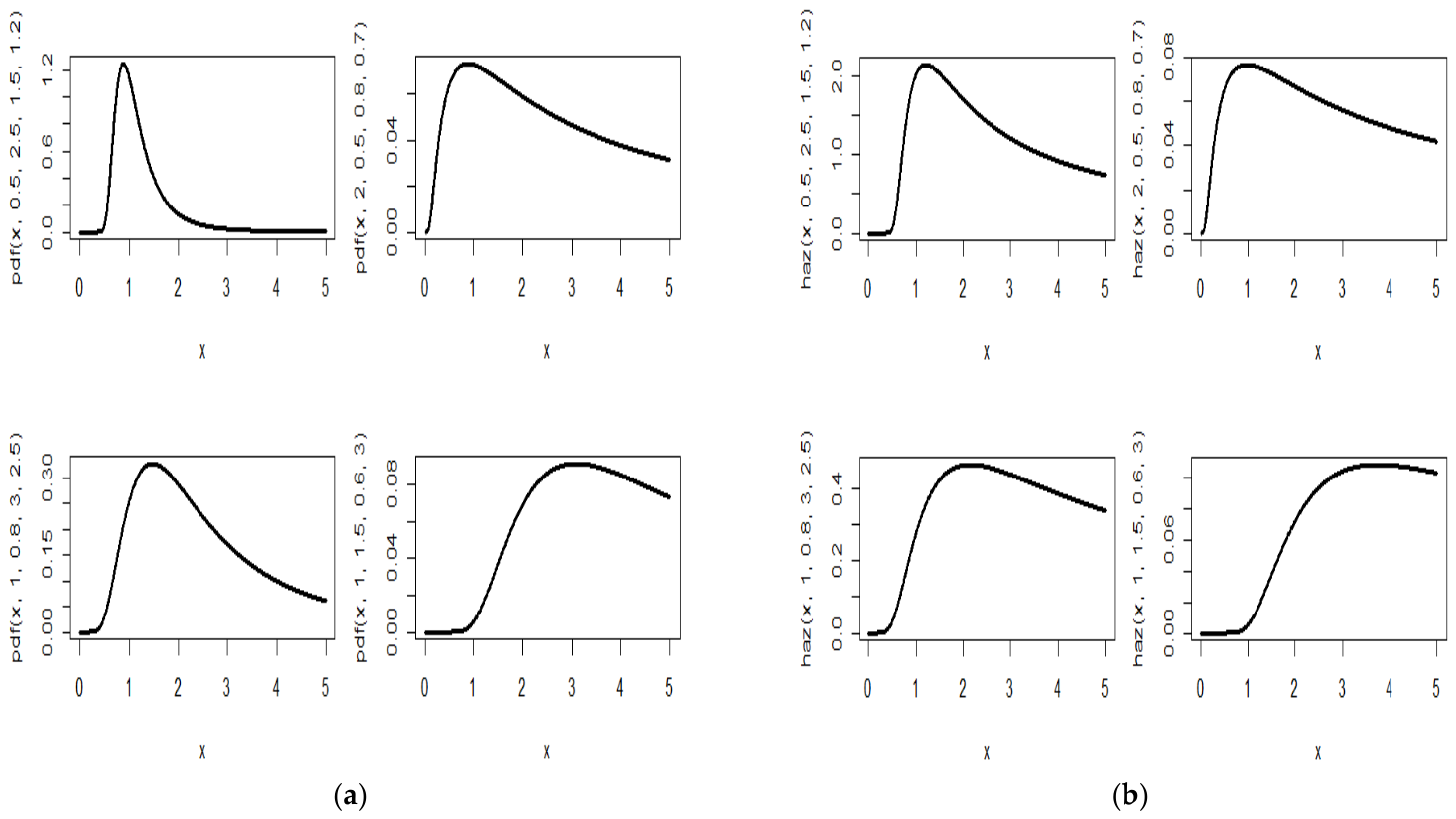
Figure 2a shows the ETIITLIW distribution’s pdf for a variety of parameter combinations, demonstrating the model’s adaptability in capturing various distributional forms. The graphs show that a wide variety of density shapes, from more dispersed and heavy-tailed structures to highly concentrated right-skewed forms, can be accommodated by the ETIITLIW distribution. Since tail behavior directly affects the estimation of extreme-loss probabilities and related risk measures, this flexibility is very useful in actuarial applications. Greater exposure to significant claims is implied by heavier tails, which raise reserve needs, premiums, solvency capital, and economic capital allocation.

Figure 2. (a) Probability density function of the ETIITLIW distribution for selected values of the parameters illustrating the flexibility of the model in capturing different degrees of skewness, tail behavior, and peak sharpness; (b) hazard rate function of the ETIITLIW distribution for selected values of the parameters illustrating its ability to capture non-monotonic (unimodal) hazard behavior under different parameter settings.

The hazard rate function for the ETIITLIW distribution for various parameter combinations is shown in Figure 2b. The plots show that the ETIITLIW distribution accommodates a wide range of non-monotonic hazard behaviors, with varying peak magnitudes and locations. This flexibility is important because it enables the model to capture diverse risk dynamics encountered in reliability, survival, and actuarial applications. From an actuarial perspective, parameter settings associated with higher hazard levels imply greater claim occurrence risk, potentially leading to higher premiums, reserve requirements, and solvency capital. Therefore, the significance of the figure lies not merely in the variety of attainable hazard shapes but in the model’s ability to represent different risk profiles within a unified and tractable framework.

Reliability Function

The reliability function of the ETIITLIW distribution is given as

$$R(x)=1-{\left[1-{\left[1-e^{-2\eta x^{-\beta }}\right]}^{\alpha }\right]}^{\theta }.$$

(46)

Hazard Function

The hazard function of the ETIITLIW distribution is given as

$$T(x)={\displaystyle \frac{2\theta \alpha \eta \beta x^{-\beta -1}{e}^{-2\eta x^{-\beta }}{\left[1-e^{-2\eta x^{-\beta }}\right]}^{\alpha -1}{\left[1-{\left[1-e^{-2\eta x^{-\beta }}\right]}^{\alpha }\right]}^{\theta -1}}{1-{\left[1-{\left[1-e^{-2\eta x^{-\beta }}\right]}^{\alpha }\right]}^{\theta }}}.$$

(47)

Quantile Function

The quantile function of the ETIITLIW distribution is given as

$$x=Q\left(u\right)={\left[{\displaystyle \frac{-1}{2\eta }}\log \left[1-{\left[1-u^{{\displaystyle \frac{1}{\theta }}}\right]}^{{\displaystyle \frac{1}{\alpha }}}\right]\right]}^{{\displaystyle \frac{-1}{\beta }}}.$$

(48)

3. Research Results and Discussions

3.1. Simulation Study

This section compares the mles’s results of the ETIITLW distribution in terms of their biases and mean square errors (MSEs) for various sample sizes. The sample sizes n = 20, 50, 100, 250, 500, and 1000 are considered, and the parameter values $(\theta =1.50,\alpha =0.50,\kappa =0.10,\phi =0.12)$ and $(\theta =2.12,\alpha =0.80,\kappa =0.20,\phi =0.22)$ are employed. The maximum likelihood approach is used to estimate the parameters in each experiment.

For each parameter configuration and sample size, we generated 1000 replications independent Monte Carlo samples. To ensure numerical stability, the optimization procedure was initialized using values close to the true parameter values employed in the data generation process. For robustness, several alternative starting values were also tested, and the resulting estimates converged to the same optimum, indicating that the likelihood surface is reasonably well behaved.

The simulation results in Table 1 provide strong empirical evidence that the maximum likelihood estimators of the ETIITLW distribution are consistent, asymptotically unbiased, and efficient. Although moderate biases are observed for small sample sizes, particularly for $\theta$ and $\phi$, these biases diminish rapidly as the sample size increases. Furthermore, the RMSE values decrease substantially across all parameters, demonstrating improved estimation precision. Consequently, the MLE method appears to be a reliable procedure for estimating the parameters of the ETIITLW distribution, especially for moderate to large sample sizes.

Table 1. Simulation results for the ETIITLW distribution.

		($\mathit{\theta }$ = 1.50, $\mathit{\alpha }$ = 0.50, $\mathit{\kappa }$ = 0.10, $\mathit{\phi }$ = 0.12)			($\mathit{\theta }$ = 2.12, $\mathit{\alpha }$ = 0.80, $\mathit{\kappa }$ = 0.20, $\mathit{\phi }$ = 0.22)
N	Parameters	Estimated Values	Bias	RMSE	Estimated Values	Bias	RMSE
20	$\theta$	1.7905	0.2905	1.9047	2.3199	0.1999	1.3411
	$\alpha$	0.7231	0.2231	0.3814	0.8320	0.0320	0.7462
	$\kappa$	0.1062	0.0062	0.0317	0.2720	0.0720	0.1033
	$\phi$	0.3102	0.1902	0.3190	0.3386	0.1186	0.3836
50	$\theta$	1.6780	0.1780	1.9002	2.1282	0.0082	1.0208
	$\alpha$	0.6373	0.1373	0.3783	0.8236	0.0236	0.6716
	$\kappa$	0.1048	0.0048	0.0272	0.2640	0.0640	0.0879
	$\phi$	0.2301	0.1101	0.3179	0.2675	0.0475	0.2971
100	$\theta$	1.5310	0.0310	1.7479	2.1247	0.0047	0.8230
	$\alpha$	0.5251	0.0251	0.3095	0.8149	0.0149	0.5551
	$\kappa$	0.1035	0.0035	0.0263	0.2556	0.0556	0.0794
	$\phi$	0.1465	0.0265	0.2822	0.2430	0.0230	0.2581
250	$\theta$	1.5104	0.0104	1.4745	2.1244	0.0044	0.4565
	$\alpha$	0.5145	0.0145	0.2826	0.8062	0.0062	0.4886
	$\kappa$	0.1024	0.0024	0.0235	0.2466	0.0466	0.0703
	$\phi$	0.1291	0.0091	0.2316	0.2305	0.0605	0.2417
500	$\theta$	1.5028	0.0025	1.4456	2.1227	0.0027	0.2667
	$\alpha$	0.5037	0.0037	0.2541	0.8026	0.0026	0.4854
	$\kappa$	0.1019	0.0019	0.0214	0.2237	0.0237	0.0642
	$\phi$	0.1211	0.0011	0.1484	0.2216	0.0016	0.1870
1000	$\theta$	1.5005	0.0005	1.3523	2.1213	0.0013	0.1759
	$\alpha$	0.5014	0.0014	0.2399	0.8014	0.0014	0.4840
	$\kappa$	0.1004	0.0004	0.0137	0.2145	0.0145	0.0582
	$\phi$	0.1200	0.0000	0.1208	0.2203	0.0003	0.1136

3.2. Applications

In this section, we check the performance of the ETIITL-G family by fitting the submodel ETIITLW distribution to two real-life datasets. We compare the ETIITLW model with some competitive distributions, including Topp-Leone Weibull (TLW) distribution by [31], Nadarajah–Haghighi (NH) distribution by [32], Kumaraswamy exponential (KE) distribution by [33], Topp-Leone exponentiated Weibull (TLEW) distribution by [34], Half-Logistic Generalized Weibull (HLGW) distribution by [35], exponentiated Fréchet (ExF) distribution by [36], Gompertz (Go) distribution by [37] and Weibull (W) distribution. These model comparators are selected since modification was carried out on the baseline Weibull distribution, and it is nice to consider some models with Weibull distribution as their baseline. We also considered some other models to test the robustness of the generated family.

The goodness-of-fit of the proposed model is evaluated using the Kolmogorov–Smirnov (K–S) and Cramér–von Mises (CvM) statistics, together with information criteria such as Akaike Information Criterion (AIC), Bayesian Information Criterion (BIC), Consistent Akaike Information Criterion (CAIC), and Hannan–Quinn Information Criterion (HQIC). The model parameters were estimated from the same data using maximum likelihood estimation, meaning that the reported K–S p-values should be interpreted as approximate rather than exact. Consequently, the K–S test is used primarily as a descriptive measure of model adequacy and should be interpreted alongside other goodness-of-fit statistics, graphical diagnostics (e.g., probability plots), and information criteria. The overall assessment of model performance is therefore based on the collective evidence from these complementary measures rather than on the K–S p-value alone.

Dataset I represents monthly measures of unemployment insurance. This data comes from the Department of Labor, Licensing, and Regulation of the State of Maryland, USA. The data was reported and used by [38]. The data are: 0.052, 0.033, 0.039, 0.050, 0.029, 0.052, 0.060, 0.032, 0.057, 0.064, 0.061, 0.064, 0.041, 0.036, 0.050, 0.053, 0.061, 0.068, 0.060, 0.050, 0.064, 0.057, 0.061, 0.059, 0.069, 0.070, 0.137, 0.170, 0.100, 0.090, 0.222, 0.109, 0.068, 0.063, 0.056, 0.090, 0.074, 0.095, 0.114, 0.133, 0.066, 0.075, 0.072, 0.054, 0.057, 0.052, 0.066, 0.069, 0.083, 0.044, 0.060, 0.080, 0.058, 0.080, 0.080, 0.052, 0.065, 0.073.

Dataset II is on services related to insurance and finance. The data cover the period from 1974 to 2021 and were reported by [34]. The dataset is presented as follows: 3.3761087, 3.7916736, 1.8623592, 2.5312656, 1.8700584, 2.6127494, 2.2765957, 2.2220998, 2.2375761, 2.3314328, 1.9051169, 4.9536694, 4.3726093, 5.9473222, 4.9426842, 7.0728029, 6.1907114, 5.0430431, 5.6950926, 2.6111077, 3.2495827, 4.6814338, 3.5658858, 2.1803091, 2.1144394, 2.5407750, 0.4822188, 1.4132725, 2.1065506, 2.2378263, 2.0468322, 2.1193183, 2.2995888, 2.0718469, 0.8246948, 10.7223221, 1.9822990, 3.7373134, 4.7968947, 3.7395944, 3.9088539, 24.7991060, 11.3768892, 9.9587088, 5.6085853.

Table 2 presents the mles for the unknown parameters and the negative log-likelihood of the ETIITLW model together with its comparators for dataset I. Also, Table 3 presents the mles for the unknown parameters and the negative log-likelihood of the ETIITLW model together with its comparators for dataset II.

Table 2. Parameter estimates and negative log-likelihood of the ETIITLW model and its comparators for dataset I.

Models	$\widehat{\mathit{\alpha }}$	$\widehat{\mathit{\theta }}$	$\widehat{\mathit{\kappa }}$	$\mathit{\phi }$	$-\mathit{l}\mathit{l}$
ETIITLW	4.7411	109.7998	5.7198	0.4489	−134.5494
NHD	-	0.0703	134.3365	-	−106.6953
KE	33.6797	71.4787	0.5535	-	−133.9225
TLW	0.5265	279.3402	12.7796	-	−134.5004
TLEW	15.3629	0.4141	13.1844	16.3019	−134.5318
W	-	294.9898	2.2498	-	−121.2192
HLGW	0.7891	2.0880	446.8134	-	−122.2323
ExF	2.6605	1.2945	0.0592	-	−133.9878
Go	6.7873	13.4512	-	-	−108.2112

Table 3. Parameter estimates of the ETIITLW model and its comparators for dataset II.

Models	$\widehat{\mathit{\alpha }}$	$\widehat{\mathit{\theta }}$	$\widehat{\mathit{\kappa }}$	$\mathit{\phi }$	$-\mathit{l}\mathit{l}$
ETIITLW	4.0561	15.5834	0.8619	0.3696	99.1804
NHD	-	0.1571	1.3307	-	108.9543
KE	5.8239	1.2389	0.2805	-	100.7332
TLW	0.4506	28.8555	1.1088	-	99.2283
TLEW	7.4552	0.3455	1.9087	5.0137	99.2111
W	-	0.1334	1.3191	-	106.3060
HLGW	0.1960	3.6957	0.4878	-	100.2822
ExF	1.6160	0.2811	0.4716	-	104.9091
Go	0.2284	0.0111	-	-	109.3713

Table 4 uses information criteria and goodness-of-fit (GOF) tests to compare the performance of multiple models (ETIITLW, EW, KE, TLW, TLEW, and W) for dataset I. With AIC = −261.0988, BIC = −252.8571, CAIC = −260.3441, and HQIC = −257.8885, the ETIITLW distribution has the lowest values for all criteria. This suggests that, of all the models, ETIITLW offers the best overall fit for dataset I. As additional support to buttress the information criteria, the goodness-of-fit statistic is employed. The ETIITLW distribution has a K–S value = 0.1185 as the lowest and p-value = 0.3899 as the largest among the competitors. The ETIITLW distribution has a CvM value = 0.1325 as the lowest and p-value = 0.4830 as the largest among the competitors. These results show that the ETIITLW distribution offers better fit for dataset I.

Table 4. Goodness-of-fit of the ETIITLW model and its comparators for dataset I.

Models	AIC	BIC	CAIC	HQIC	K–S	p-Value	CvM	p-Value
ETIITLW	−261.0988	−252.8571	−260.3441	−257.8885	0.1185	0.3899	0.1325	0.4830
NHD	−209.3907	−205.2698	−209.1725	−207.7855	0.3316	5.8 × 10−8	1.6265	7.4 × 10−5
KE	−259.8449	−251.6031	−259.0902	−256.6346	0.1143	0.3850	0.1715	0.3308
TLW	−261.0016	−252.7599	−260.2469	−257.7913	0.1193	0.3806	0.1542	0.3778
TLEW	−261.0635	−252.8218	−260.3089	−257.8532	0.1195	0.3889	0.1424	0.4147
W	−234.4385	−226.1967	−233.6838	−231.2282	0.1781	0.0506	0.6038	0.0216
HLGW	−238.4646	−232.2833	−238.0202	−236.0569	0.1845	0.0385	0.5549	0.0286
ExF	−259.0756	−251.7953	−259.5312	−256.5241	0.1398	0.2071	0.1952	0.2773
Go	−212.4225	−208.3016	−212.2043	−210.8173	0.2630	0.0007	1.1574	0.0010

Also, Table 5 uses information criteria and goodness-of-fit (GOF) tests to compare the performance of multiple models (ETIITLW, EW, KE, TLW, TLEW, and W) for dataset II. With AIC = 206.3608, BIC = 213.5874, CAIC = 207.3608, and HQIC = 209.0558, the ETIITLW distribution has the lowest values for all criteria. This suggests that, of all the models, ETIITLW offers the best overall fit for dataset II. As additional support to buttress the information criteria, the goodness-of-fit statistic is employed. The ETIITLW distribution has a K–S value = 0.1393 as the lowest and p-value = 0.3171 as the largest among the competitors. The ETIITLW distribution has a CvM value = 0.1293 as the lowest and p-value = 0.4964 as the largest among the competitors. These results show that the ETIITLW distribution offers better fit for dataset II.

Table 5. Goodness-of-fit of the ETIITLW model and its comparators for dataset II.

Models	AIC	BIC	CAIC	HQIC	K–S	p-Value	CvM	p-Value
ETIITLW	206.3608	213.5874	207.3608	209.0558	0.1393	0.3171	0.1293	0.4964
NHD	221.9087	225.5220	222.1944	223.2557	0.2677	0.0024	0.5203	0.0349
KE	209.4664	216.6931	210.4664	212.1604	0.1498	0.2396	0.1883	0.2921
TLW	206.4565	213.6832	207.4565	209.1506	0.1402	0.3096	0.1366	0.4344
TLEW	206.4220	213.6488	207.4222	209.1162	0.1387	0.3117	0.1317	0.4518
W	220.6120	227.8387	221.6120	223.3060	0.1947	0.0572	0.3425	0.1028
HLGW	208.6323	214.0523	209.2117	209.6528	0.1478	0.2532	0.1863	0.2962
ExF	215.8183	221.2382	216.4036	217.8388	0.2020	0.0437	0.2675	0.1674
Go	222.7425	226.3559	223.0283	224.0895	0.2826	0.0011	0.5875	0.0236

The correlation matrix of the ETIITLW model parameters for dataset I is displayed in Table 6, and that of dataset II is displayed in Table 7. Since every parameter has a perfect correlation with itself, it is expected that all the diagonal elements are 1.000. The linear relationship between pairs of parameters is measured by the off-diagonal elements. There is little to no linear dependence between the parameters, as all correlations are very near to zero. This is a desirable attribute from the standpoint of modeling, particularly for novel distributions, since it shows that each parameter captures unique features of the data.

Table 6. Correlation matrix of ETIITLW model for dataset I.

	$\alpha$	$\theta$	$\kappa$	$\phi$
$\alpha$	1.0000000	0.0067953	0.0055031	−0.0000223
$\theta$	0.0067953	1.0000000	0.0939122	−0.0003821
$\kappa$	0.0055031	0.0939122	1.0000000	0.0014493
$\phi$	−0.0000223	−0.0003821	0.0014493	1.0000000

Table 7. Correlation matrix of ETIITLW model for dataset II.

	$\alpha$	$\theta$	$\kappa$	$\phi$
$\alpha$	1.0000000	0.0983826	0.0086337	−0.0000211
$\theta$	0.0983826	1.0000000	0.1651603	−0.0004025
$\kappa$	0.0086337	0.1651603	1.0000000	−0.0037506
$\phi$	−0.0000211	−0.0004025	−0.0037506	1.0000000

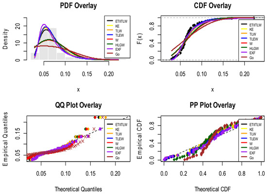
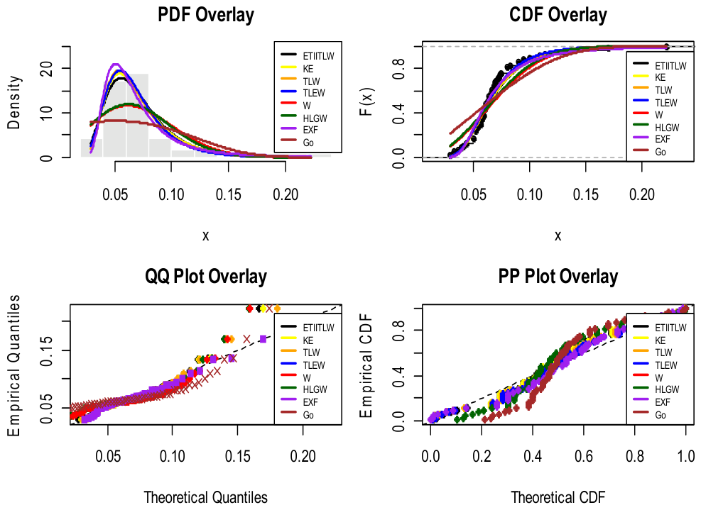
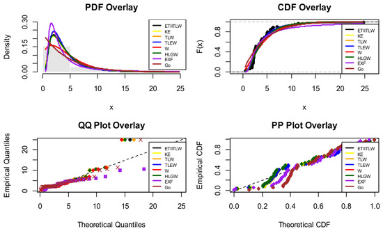
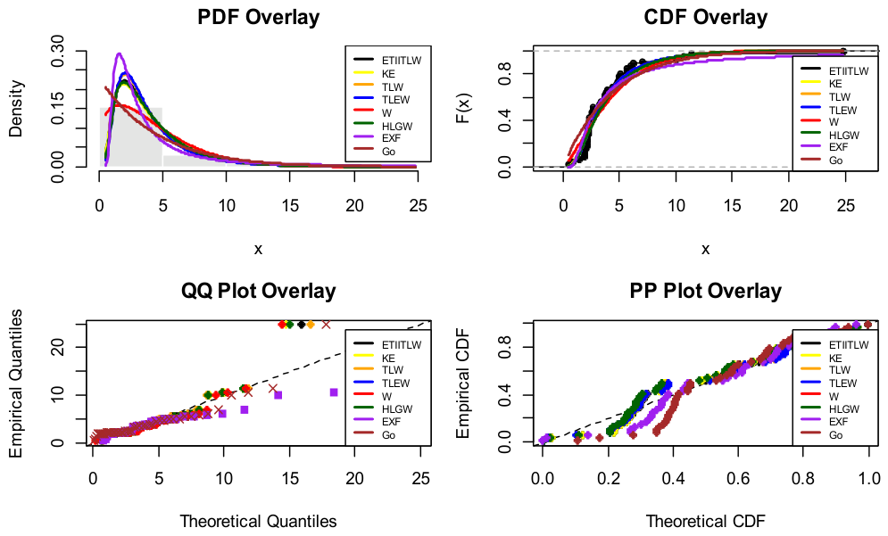
Four typical diagnostic plots are shown in Figure 3 and Figure 4 to evaluate how well a theoretical distribution that has been proposed together with its comparators fits the observed dataset I and dataset II. The empirical density, Q–Q, CDF, and P–P plots collectively demonstrate that the proposed distribution provides an adequate fit to the data, with only minor deviations observed in the upper tail, confirming its suitability for modeling insurance-type data. The PDF overlay demonstrates that the majority of the models accurately represent the main body of the data. However, there are noticeable variations in the right tail. Compared to various rival models, especially the Weibull (W), Go, and HLGW distributions, which fall more quickly, the ETIITLW density shows a heavier and more slowly fading tail. This behavior implies that the ETIITLW model is more appropriate for modeling huge insurance claims since it gives more probability mass to extreme data.

Figure 3. Plots of fitted empirical and theoretical densities, cdf, Q–Q plot and P–P plot for dataset I.

Figure 4. Plots of fitted empirical and theoretical densities, cdf, Q–Q plot and P–P plot for dataset II.

Table 8 and Table 9 show the estimated risk measures for the suggested ETIIITLW distribution and its competing models at confidence levels 90%, 95%, and 99% using the real-life datasets. These metrics, which are frequently employed in actuarial pricing, reserving, reinsurance, and solvency assessment, quantify the size and uncertainty of extreme losses. VaR, TVaR, and TVP all climb as the confidence level goes from 0.90 to 0.99 for all models. This suggests that concentrating on increasingly extreme tail events is likely to result in more severe losses. TVaR is greater than VaR for each model, indicating that the average loss over the VaR threshold is much greater than the threshold. This pattern illustrates the rising capital needs linked to higher confidence levels and is compatible with actuarial risk theory.

Table 8. Estimated risk measures for ETIITLW model and its comparators for dataset I.

Models	Level	VaR	TVaR	TV	TVP
	0.90	0.156700	0.155569	0.002069	0.152866
ETIITLW	0.95	0.165675	0.176113	0.002077	0.169821
	0.99	0.193841	0.298308	0.002803	0.228444
	0.90	0.105950	0.134905	0.001011	0.135006
TLEW	0.95	0.124771	0.155613	0.001151	0.155729
	0.99	0.173325	0.209248	0.001545	0.209402
	0.90	0.107068	0.136571	0.001021	0.136672
TLW	0.95	0.126395	0.157599	0.001140	0.157713
	0.99	0.175732	0.211271	0.001457	0.211417
	0.90	0.110551	0.131685	0.000397	0.131725
HLGW	0.95	0.125826	0.145967	0.000370	0.146005
	0.99	0.158418	0.177131	0.000328	0.177165
	0.90	0.107292	0.132634	0.000636	0.132697
KE	0.95	0.124887	0.150178	0.000635	0.150242
	0.99	0.165594	0.190858	0.000634	0.190921
	0.90	0.105769	0.136212	0.001281	0.136340
ExF	0.95	0.124894	0.158299	0.001559	0.158456
	0.99	0.176392	0.219082	0.002626	0.219345
	0.90	0.127585	0.148150	0.000284	0.148178
Go	0.95	0.143992	0.161151	0.000208	0.161171
	0.99	0.172117	0.184547	0.000118	0.184559
	0.90	0.126926	0.152759	0.000467	0.152806
NHD	0.95	0.147236	0.169281	0.000355	0.169316
	0.99	0.183364	0.199846	0.000211	0.199867
	0.90	0.115660	0.134493	0.000272	0.134520
W	0.95	0.130011	0.146798	0.000224	0.146820
	0.99	0.157391	0.171157	0.000160	0.171173

Table 9. Estimated risk measures for ETIITLW model and its comparators for dataset II.

Models	Level	VaR	TVaR	TV	TVP
	0.90	9.814840	12.738137	22.522626	13.990399
ETIITLW	0.95	12.211397	15.625238	27.904507	17.415689
	0.99	19.045172	24.729216	44.095130	27.1387292
	0.90	7.801744	11.772700	23.633050	14.136010
TLEW	0.95	10.210017	14.703440	29.61270	17.66471
	0.99	17.145739	23.014170	48.016750	27.815850
	0.90	7.8569964	11.766712	21.659747	13.932687
TLW	0.95	10.265356	14.634226	26.401022	17.274328
	0.99	17.060947	22.576292	39.945189	26.570811
	0.90	8.0760896	11.228114	11.143932	12.342507
HLGW	0.95	10.178450	13.455943	12.003307	14.656273
	0.99	15.396645	18.971699	14.051020	20.376802
	0.90	7.7854221	11.053137	20.211231	11.110390
KE	0.95	10.098622	14.965231	25.01302	15.241567
	0.99	17.450170	22.729216	41.295211	23.887291
	0.90	7.7695633	11.850202	21.920680	12.742270
ExF	0.95	10.174289	14.893818	25.846110	16.778429
	0.99	17.300109	23.958192	42.853623	26.643555
	0.90	9.558831	13.339250	13.222220	14.661480
Go	0.95	12.248675	15.92226	12.51101	17.17336
	0.99	18.201410	21.64882	11.06507	22.75533
	0.90	9.2606451	12.613079	10.203504	13.633430
NHD	0.95	11.666261	14.891123	9.5562567	15.846748
	0.99	16.889050	19.891288	8.4385032	20.735138
	0.90	8.6654484	11.308629	6.2015929	11.928789
W	0.95	10.578778	13.094701	5.7244914	13.667150
	0.99	14.655829	16.965747	4.953292	17.461077

In terms of pricing, the ETIITLW distribution gives higher TVP than its comparators, implying higher risk loading, and higher TVaR implies larger reserves for extreme claims. For solvency, higher VaR implies greater capital held against insolvency, and for capital allocation, high TV indicates more uncertainty in catastrophic losses, implying more economic capital allocated to risky portfolios.

4. Conclusions and Recommendations

This research study developed and studied a new family of distributions called the exponentiated type II Topp-Leone-G family of distributions. The family is derived using the T-X methodology. The exponentiated family of distributions as baseline served as the transformer (T), and type II Topp-Leone-G served as the transformed (X). The ETIITL-G extends the TIITL-G by introducing an exponentiation mechanism that enhances the tail behavior and skewness control; provides greater flexibility in the hazard rate structure; and allows diverse density shapes, including right-skewed, symmetric, bathtub, inverted bathtub and non-monotonic hazard functions. This flexibility represents a meaningful advancement over classical models, such as Weibull, exponential, Gamma, inverse Weibull, inverse exponential and many other models whose hazard structures are often restrictive.

The density expansion of the exponentiated type II Topp-Leone-G family of distributions is done from which some of the properties are obtained. The properties of the exponentiated type II Topp-Leone-G family of distributions include moments, moment generating function, quantile function, reliability function, hazard function, order statistics, and Rényi entropy, and actuarial measures are examined as statistical components of the exponentiated type II Topp-Leone-G family of distributions. The maximum likelihood estimation method is used to estimate the unknown parameters of the model. As baseline distributions, two submodels, Weibull and inverse Weibull distributions, are used to illustrate the family’s form and evaluate its fit. The Weibull distribution is used as the baseline distribution in a simulation study to assess the performance of the new distribution. This is to evaluate the effectiveness of the employed maximum likelihood estimation technique. To determine the significance and adaptability of the exponentiated type II Topp-Leone-G family of distributions, two real-world datasets are used. The findings show that the exponentiated type II Topp-Leone Weibull distribution seems to offer better fit than the competing models under consideration for the data analyzed. This suggests that the exponentiated type II Topp-Leone-G family of distributions has added more flexibility to the baseline distribution.

The strength of the empirical validation is reflected through the lower values of the information criterion, such as AIC, BIC, CAIC, and HQIC. The strength of the empirical evidence is also reflected through a better goodness-of-fit statistic, such as K–S and CvM, together with their corresponding p-values and superior graphical fittings. The consistency and efficiency of the maximum likelihood estimators under varying sample sizes further strengthen the credibility of the proposed model.

Although the observed improvements in AIC, BIC, CAIC, HQIC, KS, and CvM statistics are sometimes numerically small, their practical implications should not be underestimated. In many actuarial and reliability applications, decisions depend heavily on accurate estimation of extreme quantiles and tail behavior. Small improvements in overall model fit may lead to noticeable differences in estimated risk measures, survival probabilities, hazard rates, and capital requirements. Therefore, the superiority of the proposed model is not solely reflected in statistical criteria but also in its potential to enhance decision-making in risk-sensitive environments.

The research derived some actuarial measures, such as VaR, TVaR, TV, and TVP, and the value of the measures were computed with standard confidence levels of 90%, 95% and 99% using the real-life datasets. The results were compared with the competing models. The findings from the analysis, which are displayed in Table 8 and Table 9, demonstrated that the proposed ETIIITLW distribution is better at capturing extreme-loss behavior, as seen by its consistently higher VaR, TVaR, TV, and TVP values at high confidence levels. These results show that the model offers a more thorough depiction of tail risk than the competing distributions, which makes it especially appropriate for actuarial applications, including capital allocation, reinsurance design, insurance pricing, and solvency risk management. More reliable and financially sound actuarial decision-making is supported by its capacity to measure the extent and variability of extreme losses.

The computationally tractable representations for VaR and TVaR enhance the practical utility of the model by facilitating the quantification of extreme losses and tail risk. These measures are fundamental tools for insurance pricing, capital allocation, solvency assessment, reserve determination, and enterprise risk management under regulatory frameworks. The model therefore offers a useful framework for evaluating both the frequency and severity of rare but high-impact events, making it suitable for applications involving insurance claims, financial losses, and operational risks. Although the empirical results demonstrate promising performance on the datasets analyzed, further validation using larger and more diverse actuarial datasets would help establish its broader applicability. Future research may extend the proposed distribution to regression settings, multivariate frameworks, Bayesian inference, and machine learning-based risk prediction models, thereby broadening its usefulness for modern actuarial and financial risk management.

References

- Hardy, M.R. An Introduction to Risk Measures for Actuarial Applications, SOA Syllabus Study Note. 2006. Available online: www.soa.org/globalassets/assets/files/edu/c-25-07.pdf (accessed on 2 April 2026).
- Embrechts, P.; Wüthrich, M.V. Recent challenges in actuarial science. Annu. Rev. Stat. Its Appl. 2022, 9, 119–140. [Google Scholar] [CrossRef] [Scilit]
- Ahmad, Z.; Mahmoudi, E.; Dey, S. A new family of heavy tailed distributions with an application to the heavy tailed insurance loss data. Commun. Stat. Simul. Comput. 2022, 51, 4372–4395. [Google Scholar] [CrossRef] [Scilit]
- Zichuan, M.; Hussain, S.; Iftikhar, A.; Ilyas, M.; Ahmad, Z.; Khan, D.M.; Manzoor, S. A New Extended X Family of Distributions: Properties and Applications. Comput Math. Methods Med. 2020, 2020, 4650520. [Google Scholar] [CrossRef] [Scilit] [PubMed] [PubMed Central]
- Atchadé, M.N.; N’bouké, M.; Djibril, A.M.; Shahzadi, S.; Hussam, E.; Aldallal, R.; Alshanbari, H.M.; Gemeay, A.M.; El-Bagoury, A.H. A New Power Topp-Leone distribution with applications to engineering and industry data. PLoS ONE 2023, 18, e0278225. [Google Scholar] [CrossRef] [Scilit] [PubMed] [PubMed Central]
- Ahmad, Z.; Mahmoudi, E.; Alizadeh, M.; Roozegar, R.; Afify, A.Z. The Exponential T-X Family of Distributions: Properties and an Application to Insurance Data. J. Math. 2021, 2021, e3058170. [Google Scholar] [CrossRef] [Scilit]
- Bello, O.A.; Doguwa, S.I.; Yahaya, A.; Haruna, M.J. A Type I Half Logistic Exponentiated –G family of distribution: Properties and applications. Commun. Phys. Sci. 2021, 7, 147–163. [Google Scholar]
- Falgore, J.Y.; Doguwa, S.I. The Inverse Lomax-G Family with application to Breaking Strength Data. Asian J. Probab. Stat. 2020, 8, 49–60. [Google Scholar] [CrossRef] [Scilit]
- Atchadé, M.N.; N’bouké, M.A.G.; Djibril, A.M.; Mutairi, A.A.L.; Mustafa, M.S.; Hussam, E.; Alsuhabi, H.; Nassr, S.G. A new Topp-Leone Kumaraswamy Marshall-Olkin generated family of distributions with applications. Heliyon 2024, 10, e24001. [Google Scholar] [CrossRef] [Scilit] [PubMed]
- Atchadé, M.N.; Otodji, T.; Djibril, A.M.; N’bouké, M. Power Topp–Leone exponential negative family of distributions with numerical illustrations to engineering and biological data. Open Phys. 2023, 21, 20230151. [Google Scholar] [CrossRef] [Scilit]
- Belili, M.C.; Alshangiti, A.M.; Gemeay, A.M.; Zeghdoudi, H.; Karakaya, K.; Bakr, M.E.; Balogun, O.S.; Atchadé, M.N.; Hussam, E. Two-parameter family of distributions: Properties, estimation, and applications. AIP Adv. 2023, 13, 105008. [Google Scholar] [CrossRef] [Scilit]
- Abdelall, Y.Y.; Hassan, A.; Almetwally, E. A new extension of the odd inverse Weibull-g family of distributions: Bayesian and non-Bayesian estimation with engineering applications. Comput. J. Math. Stat. Sci. 2024, 3, 359–388. [Google Scholar] [CrossRef] [Scilit]
- Algarni, A.; Almarashi, A.M.; Jamal, F.; Chesneau, C.; Elgarhy, M. Truncated Inverse Lomax Generated Family of Distributions with Applications to Biomedical Data. J. Med. Imaging Health Inform. 2021, 11, 2425–2439. [Google Scholar] [CrossRef]
- Ibrahim, S.; Doguwa, S.I.; Audu, I.; Jibril, H.M. On the Topp Leone exponentiated-G Family of Distributions: Properties and Applications. Asian J. Probab. Stat. 2020, 7, 1–15. [Google Scholar] [CrossRef] [Scilit]
- Ibrahim, S.; Doguwa, S.I.; Isah, A.; Haruna, J.M. The Topp Leone Kumaraswamy-G Family of Distributions with Applications to Cancer Disease Data. J. Biostat. Epidemiol. 2020, 6, 37–48. [Google Scholar] [CrossRef] [Scilit]
- Sule, I.; Bello, O.A.; Kolawole, I.A. A new Generalized Exponentiated Family of Continuous Distributions with Applications to Environmental Data Sets. Reliab. Theory Appl. 2025, 20, 38–52. [Google Scholar]
- Al-Shomrani, A.; Arif, O.; Shawky, A.; Hanif, S.; Shahbaz, M.Q. Topp-Leone family of distributions: Some properties and application. Pak. J. Stat. Oper. Res. 2016, 12, 443–451. [Google Scholar] [CrossRef] [Scilit]
- Aljohani, H.M.; Bandar, S.A.; Al-Mofleh, H.; Ahmad, Z.; El-Morshedy, M. Correction: A new asymmetric extended family: Properties and estimation methods with actuarial applications. PLoS ONE 2024, 19, e0315953. [Google Scholar] [CrossRef] [Scilit] [PubMed]
- Elgarhy, M.; Arslan Nasir, M.; Jamal, F.; Ozel, G. The Type II Topp-Leone Generated family of distributions: Properties and applications. J. Stat. Manag. Syst. 2018, 21, 1529–1551. [Google Scholar] [CrossRef] [Scilit]
- Gupta, R.C.; Gupta, P.L.; Gupta, R.D. Modeling failure time data by Lehmann alternatives. Commun. Stat. Theory Methods 1998, 27, 887–904. [Google Scholar] [CrossRef] [Scilit]
- Alzaatreh, A.; Lee, C.; Famoye, F. A new method for generating families of continuous distributions. Metron 2013, 71, 63–79. [Google Scholar] [CrossRef] [Scilit]
- Rényi, A. On measures of entropy and information. In Proceedings of the Fourth Berkeley Symposium on Mathematical Statistics and Probability–I; University of California Press: Berkeley, CA, USA, 1961; pp. 547–561. [Google Scholar]
- Artzner, P. Application of coherent risk measures to capital requirements in insurance. N. Am. Actuar. J. 1999, 3, 11–25. [Google Scholar] [CrossRef] [Scilit]
- Klugman, S.A.; Panjer, H.H.; Willmot, G.E. Loss Models: From Data to Decisions, 4th ed.; John Wiley & Sons: Hoboken, NJ, USA, 2012; pp. 42–43. [Google Scholar]
- Landsman, Z. On the tail mean-variance optimal portfolio selection. Insur. Math. Econ. 2010, 46, 547–553. [Google Scholar] [CrossRef] [Scilit]
- Furman, E.; Landsman, Z. Tail variance premium with applications for elliptical portfolio of risks. ASTIN Bull. J. IAA 2006, 36, 433–462. [Google Scholar] [CrossRef] [Scilit]
- R Core Team. R: A Language and Environment for Statistical Computing; R Foundation for Statistical Computing: Vienna, Austria, 2025; Available online: https://www.R-project.org/ (accessed on 5 June 2026).
- Weibull, W. A Statistical Distribution Function of Wide Applicability. J. Appl. Mech. 1951, 18, 293–297. [Google Scholar] [CrossRef] [Scilit]
- Keller, A.Z.; Kamath, A.R.R. Alternative reliability models for mechanical systems. In Proceedings of the Third International Conference on Reliability and Maintainability, Toulse, France, 18–22 October 1982. [Google Scholar]
- Nelson, W.B. Applied Life Data Analysis; Wiley: New York, NY, USA, 1982. [Google Scholar]
- Tuoye, D.O.; Opone, F.C.; Ekhosuehi, N. Topp-Leone Weibull Distribution. Earthline J. Math. Sci. 2021, 7, 381–401. [Google Scholar] [CrossRef] [Scilit]
- Nadarajah, S.; Haghighi, F. An extension of the exponential distribution. Statistics 2011, 45, 543–558. [Google Scholar] [CrossRef] [Scilit]
- Adepoju, K.A.; Chukwu, O.I. Maximum Likelihood Estimation of the Kumaraswamy Exponential Distribution with Applications. J. Mod. Appl. Stat. Methods 2015, 14, 18. [Google Scholar] [CrossRef] [Scilit]
- Ibrahim, S. The properties of Topp-Leone exponentiated Weibull distribution with application to survival data. Res. J. Math. Stat. Sci. 2021, 9, 9–15. [Google Scholar]
- Masood, A.; Amna, B. The Half-Logistic Generalized Weibull Distribution. J. Probab. Stat. 2018, 8767826, 12. [Google Scholar] [CrossRef] [Scilit]
- Nadarajah, S.; Kotz, S. The Exponentiated Fréchet Distribution. Interstat Electron. J. 2003, 14, 1–7. [Google Scholar]
- Gompertz, B. On the nature of the function expressive of the law of human mortality, and on a new mode of determining the value of life contingencies. Philos. Trans. R. Soc. Lond. 1825, 115, 513–583. [Google Scholar] [CrossRef] [Scilit]
- Atchadé, M.N.; Kossou, E.Z.; Otodji, T.; Bogninou, M.J.; Djibri, A.M. Modeling Economics and Finance Data with the Arctan Marshall-Olkin Weibull Distribution. Ann. Data Sci. 2025, 1–34. [Google Scholar] [CrossRef] [Scilit]
Disclaimer/Publisher’s Note: The statements, opinions and data contained in all publications are solely those of the individual author(s) and contributor(s) and not of MDPI and/or the editor(s). MDPI and/or the editor(s) disclaim responsibility for any injury to people or property resulting from any ideas, methods, instructions or products referred to in the content. |
© 2026 by the authors. Licensee MDPI, Basel, Switzerland. This article is an open access article distributed under the terms and conditions of the Creative Commons Attribution (CC BY) license.