On the Analytical Solutions and Conservation Laws of the Special Extended Korteweg–De Vries Equation

Abstract

We study a special case of the extended Korteweg–de Vries (eKdV) equation, arising in the description of weakly nonlinear long waves with higher-order dispersive effects. The model incorporates both third- and fifth-order dispersion and quadratic nonlinearity and describes steeper and shorter waves than the classical KdV equation. First, we determine the Lie point symmetry algebra of the equation and show that it reduces to space–time translations, which in turn motivates a traveling-wave reduction. The reduced fifth-order ODE is then analyzed by means of a calibrated $(G^{\prime }/G)$-expansion ansatz. Although homogeneous balance suggests a degree $M=4$ for exact solutions, a degree-$M=2$ truncation already yields three coherent families of traveling waves—hyperbolic (solitary), trigonometric (periodic), and rational—distinguished by the discriminant of the auxiliary linear equation. Using the direct multiplier method, we construct four conservation laws, corresponding to mass, momentum, energy, and a higher-order dispersion invariant, with all ${\alpha }^2$ contributions retained. Direct substitution and numerical diagnostics demonstrate that, once the algebraic wave speed is imposed, the $M=2$ profiles satisfy the PDE with residuals of order ${10}^{-3}$ and preserve the conserved quantities to machine precision (below ${10}^{-13}\%$ relative variation) over extended integration domains. These results extend the known solution structure of the special eKdV equation and illustrate the effectiveness of the $(G^{\prime }/G)$ framework for higher-order dispersive models.

1. Introduction

The study of nonlinear evolution equations (NLEEs) remains a central task in nonlinear science due to their ubiquitous appearance in modeling complex phenomena across physics, engineering, and applied mathematics. Among these equations, the Korteweg–de Vries (KdV) equation and its various generalizations have attracted sustained attention for over a century due to their remarkable mathematical structure and physical applicability [1,2].

The classical Korteweg–de Vries equation,

$$u_t+6u{u}_x+u_{xxx}=0,$$

models weakly nonlinear long waves in dispersive media, where the first-order nonlinear term $6u{u}_x$ is balanced by the third-order dispersive term $u_{xxx}$ [2,3]. This equation has been extensively studied and is known to be completely integrable, possessing infinitely many conservation laws and soliton solutions, and admitting solution via the inverse scattering transform [4,5].

However, in many physical situations, the KdV approximation becomes insufficient when waves become steeper or have shorter wavelengths. In such regimes, higher-order nonlinear and dispersive terms must be retained, leading to extended or modified KdV equations [6,7]. The extended Korteweg–de Vries (eKdV) equation incorporates these higher-order corrections and takes the general form

$$u_t+u_x+\alpha (\lambda u{u}_x+u_{xxx})+{\alpha }^2(c_1{u}^2{u}_x+c_2{u}_x{u}_{xx}+c_{3}u{u}_{xxx}+c_4{u}_{xxxxx})=0,$$

where $\alpha$ is a non-dimensional small parameter measuring wave amplitude and $c_1,c_2,c_3,c_4,\lambda$ are coefficients depending on the physical context [6].

The special case obtained by setting $c_1=45$, $c_2=c_3=15$, $c_4=1$, and $\lambda =6$ yields

$$u_t+u_x+\alpha (6u{u}_x+u_{xxx})+{\alpha }^2(u_{xxxxx}+15u{u}_{xxx}+15u_{xx}{u}_x+45u^2{u}_x)=0.$$

(1)

This equation is particularly interesting because it combines third-order ($u_{xxx}$) and fifth-order ($u_{xxxxx}$) linear dispersion in a way that is absent from standard fifth-order KdV-type models; its specific coefficients hint at a link with integrable structures; and it arises naturally in shallow-water modeling beyond the classical KdV approximation [7].

From a modeling viewpoint, $u(x,t)$ denotes the free-surface elevation (or a proxy variable) over a one-dimensional spatial domain, with $x\in \mathbb{R}$ and $t\ge 0$. The small parameter $\alpha$ quantifies wave steepness, while $\lambda$ and $c_1,\dots ,c_4$ encode higher-order dispersive and nonlinear corrections inherited from long-wave asymptotics. The particular choice in (1) isolates a structurally rich higher-order KdV-type model in which third- and fifth-order dispersion coexist with quadratic nonlinearity. In what follows we focus on traveling waves and conserved quantities of this special case, motivated both by its analytical tractability and by the relevance to shallow-water regimes beyond the leading-order KdV description.

Despite the physical relevance of extended KdV equations, the special case (1) has received comparatively little attention. Building on the above context, this work makes four main contributions. First, we determine the Lie point symmetry algebra of (1) and construct the symmetry-invariant (traveling-wave) reduction. Second, we obtain explicit traveling-wave families via a calibrated $(G^{\prime }/G)$-expansion with degree $M=2$, with hyperbolic, trigonometric, and rational profiles distinguished by the auxiliary discriminant. Third, we derive conservation laws with complete ${\alpha }^2$ contributions using the direct multiplier method (mass, momentum, energy, higher-order dispersion invariant). Fourth, we verify the profiles by direct substitution and conservation diagnostics and discuss the physical interpretation within shallow-water wave theory.

Throughout, $u_t=\partial u/\partial t$ and $u_x=\partial u/\partial x$, with higher derivatives denoted similarly. We use $\alpha >0$ as the long-wave amplitude parameter and $(\lambda ,c_1,\dots ,c_4)$ as fixed coefficients determined by the asymptotic model; unless stated otherwise, we work with the special choice in (1).

The remainder of the paper is organized as follows. Section 2 reviews related work and positions our contribution within the existing literature. Section 3 presents the Lie symmetry analysis and the resulting traveling-wave reduction. Section 4 constructs explicit traveling-wave families using the $(G^{\prime }/G)$ method. Section 5 derives conservation laws via the multiplier method. Section 6 verifies the solutions and examines their consistency with the conservation laws. Section 7 discusses qualitative behaviour. Section 8 concludes and outlines directions for future research.

2. Literature Review

Numerous analytical methods have been developed for finding exact solutions of NLEEs. The inverse scattering transform [4,5] provides a powerful framework for completely integrable systems. The Hirota bilinear method [8] enables systematic construction of multi-soliton solutions. Bäcklund transformations [9,10] establish connections between solutions and often reveal hidden symmetries. Among algebraic methods, the tanh method [11], the exp-function method [12], and the simplest equation method [13,14] have proven effective for traveling wave solutions.

The $(G^{\prime }/G)$-expansion method [15,16,17], which we employ here, has emerged as a particularly versatile technique, yielding diverse solution families through a unified framework. This method has been successfully applied to various fifth-order KdV equations [18,19]. Unlike methods that seek specific solution types, the $(G^{\prime }/G)$-expansion naturally produces hyperbolic, trigonometric, and rational solutions depending on parameter values.

Lie symmetry analysis [20,21,22] remains fundamental as it provides a systematic approach to finding symmetries and constructing new solutions from known ones. The method has been successfully applied to various KdV-type equations [23,24].

For conservation laws, the direct method, Noether’s theorem [25], and the multiplier method [26] are primary approaches. The multiplier method is particularly useful for equations without a Lagrangian formulation [26,27].

Beyond third-order KdV, several fifth-order KdV-type models capture higher-order dispersion and have been extensively studied. The Kawahara equation [28] augments KdV with a fifth-order linear dispersion term and supports oscillatory solitary waves and dispersive tails. Two completely integrable fifth-order equations, the Sawada–Kotera (SK) and the Kaup–Kupershmidt (KK) equations, admit Lax-pair and bi-Hamiltonian structures and possess multi-soliton solutions via Hirota’s method [8]. These models provide useful points of comparison for the special eKdV Equation (1), which couples third- and fifth-order dispersion with specific nonlinearities not reducible to SK/KK by simple scalings.

From the perspective of mathematical structure, conservation laws for KdV-type hierarchies have been systematically developed since the early inverse-scattering works [4,5], and direct multiplier-based derivations remain effective in non-variational settings [26,27]. For solution construction, the $(G^{\prime }/G)$ framework complements both Hirota’s bilinear formalism and the inverse scattering transform [5,8,15,16,17], and it has been used for fifth-order KdV variants [14,18].

Recent analytical soliton studies also stress the need to combine explicit solution construction with stability, conservation-law, and physical interpretation checks rather than reporting formulae alone. In this direction, recent work on fractional optical soliton structures [29], conservation laws and soliton stability for higher-order nonlinear Schrödinger-type models [30], and nonlinear-media wave propagation in higher-dimensional spin-chain systems [31] provides useful benchmarks for the present revision. These references are not direct replacements for a special eKdV analysis, but they highlight current expectations: state the physical regime, identify the novelty of the analytical branch, verify conservation laws, and acknowledge stability limitations.

To address the exact-dispersion point, we also distinguish the present special eKdV model from KdV-type equations constructed to preserve the exact linear water-wave dispersion relation. For example, Karjanto [32] studied a KdV-type equation with exact dispersion and used strained-parameter ideas to describe nonlinear wave interactions. That line of work is important for retaining a prescribed dispersion relation over a broad wavenumber range. The present study has a different aim: we fix the special higher-order eKdV coefficients in (1), analyze its point symmetries, construct calibrated traveling-wave branches, and derive low-order conservation laws. Thus, the exact-dispersion literature provides useful perspective, but our equation is not assumed to possess an exact-dispersion operator, Lax pair, or complete integrability structure.

Within this literature, the coefficient choice in (1) has been little explored; here we document its symmetry content, calibrated $(G^{\prime }/G)$ traveling-wave profiles, and low-order conservation laws, and we place the resulting dynamics alongside SK/KK/Kawahara-type behaviors. Compared with studies devoted only to explicit formula generation, the present manuscript emphasizes a combined workflow: model positioning, invariant reduction, profile construction, conservation-law checks, residual diagnostics, and a clear statement of limitations.

3. Lie Symmetry Analysis

Lie symmetry methods provide a systematic framework for finding symmetries of differential equations and using them to construct exact solutions [20,21]. In this section, we determine the Lie point symmetry algebra of the special eKdV Equation (1).

This calculation is included deliberately even though the resulting algebra is small: it establishes that the special coefficient choice does not admit a hidden point-scaling reduction and that the natural invariant solutions are traveling waves. Nonclassical, potential, and generalized symmetries are not excluded by this point-symmetry computation; they require a separate analysis and are identified as future work below. This distinction is important because several fifth-order KdV-type equations possess richer generalized symmetry hierarchies even when their point symmetries are limited.

3.1. Determination of Lie Point Symmetries

Consider the one-parameter Lie group of infinitesimal transformations

$$\begin{array}{cc}\hfill \tilde{t}& =t+ϵ{\xi }^1(x,t,u)+O\left({ϵ}^2\right),\hfill \\ \hfill \tilde{x}& =x+ϵ{\xi }^2(x,t,u)+O\left({ϵ}^2\right),\hfill \\ \hfill \tilde{u}& =u+ϵ\eta (x,t,u)+O\left({ϵ}^2\right),\hfill \end{array}$$

where $ϵ$ is the group parameter. The corresponding vector field is

$$V={\xi }^1(x,t,u){\displaystyle \frac{\partial }{\partial t}}+{\xi }^2(x,t,u){\displaystyle \frac{\partial }{\partial x}}+\eta (x,t,u){\displaystyle \frac{\partial }{\partial u}}.$$

Determining Equations. Applying the fifth prolongation ${\mathrm{pr}}^{\left(5\right)}V$ to Equation (1) and requiring

$${\mathrm{pr}}^{\left(5\right)}{V\left[\mathcal{E}\right]|}_{\mathcal{E}=0}=0,$$

where $\mathcal{E}$ denotes the left-hand side of (1), yields an overdetermined system of PDEs for ${\xi }^1,{\xi }^2,\eta$.

For point symmetries (where ${\xi }^i,\eta$ depend on $x,t,u$ but not on derivatives), separating by powers of derivatives gives the following determining equations:

$$\begin{array}{cc}\hfill & {\xi }_u^2=0,{\xi }_u^1=0,{\xi }_x^1=0,{\eta }_{uu}=0,\hfill \end{array}$$

(2)

$$\begin{array}{cc}\hfill & {\eta }_u-5{\xi }_x^2=0,{\eta }_x+{\eta }_u=0,{\eta }_{xu}-2{\xi }_{xx}^2=0,\hfill \end{array}$$

(3)

$$\begin{array}{cc}\hfill & 6u{\eta }_x+{\eta }_{xxx}=0,{\xi }_t^1-{\eta }_u=0,{\xi }_t^1-{\xi }_x^2-{\xi }_t^2=0.\hfill \end{array}$$

(4)

Solution of the Determining System. From ${\xi }_u^1={\xi }_x^1=0$, we have ${\xi }^1={\xi }^1\left(t\right)$. From ${\xi }_u^2=0$, ${\xi }^2={\xi }^2(x,t)$. From ${\eta }_{uu}=0$, $\eta =a(x,t)u+b(x,t)$ for some functions $a,b$.

Substituting into (3) and equating coefficients of u:

$$a-5{\xi }_x^2=0\Rightarrow a=5{\xi }_x^2.$$

From ${\eta }_x+{\eta }_u=0$:

$$a_{x}u+b_x+a=0\Rightarrow a_x=0,b_x+a=0.$$

Thus $a=c$ (constant) and $b_x=-c$, giving $b=-cx+d\left(t\right)$.

From Equation (4) and the condition $6u{\eta }_x+{\eta }_{xxx}=0$, substituting $\eta =cu+(-cx+d(t\left)\right)$:

$$6u(-c)+0=0\Rightarrow c=0.$$

Hence $\eta =d\left(t\right)$. From ${\xi }_t^1={\eta }_u=0$, we have ${\xi }^1=c_1$ (constant).

From ${\xi }_t^1-{\xi }_x^2-{\xi }_t^2=0$ with ${\xi }^1=c_1$:

$$0-{\xi }_x^2-{\xi }_t^2=0\Rightarrow {\xi }_x^2=-{\xi }_t^2.$$

For point symmetries, we seek solutions independent of u. The simplest solutions are ${\xi }^2=c_2$ (constant) and $\eta =0$.

We also tested for scaling symmetries of the form ${\xi }^1=at$, ${\xi }^2=bx$, $\eta =cu$. Substitution into the determining equations gives $c=5b$, while the structure of the fifth-order terms forces $b=0$; hence $a=b=c=0$ and no nontrivial scaling symmetry is admitted.

Theorem 1. 

The special eKdV Equation (1) admits the two-dimensional Lie algebra of point symmetries spanned by

$$\begin{array}{cc}\hfill V_1& ={\displaystyle \frac{\partial }{\partial t}},\hfill \\ \hfill V_2& ={\displaystyle \frac{\partial }{\partial x}}.\hfill \end{array}$$

Proof. 

Let $V={\xi }^1(x,t,u){\partial }_t+{\xi }^2(x,t,u){\partial }_x+\eta (x,t,u){\partial }_u$ be a point-symmetry generator and let $\mathcal{E}$ denote the left-hand side of (1). The invariance condition ${\mathrm{pr}}^{\left(5\right)}V\left[\mathcal{E}\right]{|}_{\mathcal{E}=0}=0$ yields the determining Equations (2)–(4).

From (2) we obtain ${\xi }^1={\xi }^1\left(t\right)$, ${\xi }^2={\xi }^2(x,t)$ and $\eta =a(x,t)u+b(x,t)$. The relations in (3) give $a=5{\xi }_x^2$, $a_x=0$, $b_x=-a$, and ${\xi }_{xx}^2=0$. Hence

$${\xi }^2(x,t)=p\left(t\right)x+q\left(t\right),a\left(t\right)=5p\left(t\right),b(x,t)=-5p\left(t\right)x+d\left(t\right).$$

Using (4), ${\xi }_t^1={\eta }_u=a=5p\left(t\right)$ and ${\xi }_t^1-{\xi }_x^2-{\xi }_t^2=0$ imply $p^{\prime }\left(t\right)=0$ and $q^{\prime }\left(t\right)=4p\left(t\right)$. Consequently,

$${\xi }^1=5p_{0}t+c_1,{\xi }^2=p_{0}x+4p_{0}t+c_2,\eta =5p_{0}u-5p_{0}x+d\left(t\right),$$

with constants $p_0,c_1,c_2$ and some function $d\left(t\right)$.

Substituting these expressions into ${\mathrm{pr}}^{\left(5\right)}V\left[\mathcal{E}\right]{|}_{\mathcal{E}=0}=0$ and equating coefficients of independent differential monomials forces $p_0=0$ and $d^{\prime }\left(t\right)=0$. In particular, the coefficient of the cubic nonlinearity $u^2{u}_x$ is proportional to $p_0$ and thus vanishes only when $p_0=0$; with $p_0=0$, the coefficient of $u_x$ reduces to $d^{\prime }\left(t\right)$ and hence $d^{\prime }\left(t\right)=0$. The remaining constant shift d is excluded by the quadratic term $6u{u}_x$, so $d\equiv 0$. Therefore ${\xi }^1=c_1$, ${\xi }^2=c_2$, and $\eta \equiv 0$; i.e., the only point symmetries are time and space translations generated by $V_1$ and $V_2$. Since $[V_1,V_2]=0$, the Lie algebra is abelian. □

3.2. Group-Invariant Solutions

Because the Lie algebra is spanned by the translation symmetries, any constant linear combination remains a symmetry generator. We therefore introduce

$$V_c=V_1+c{V}_2={\partial }_t+c{\partial }_x,c\in \mathbb{R},$$

whose characteristic equations read

$${\displaystyle \frac{dt}{1}}={\displaystyle \frac{dx}{c}}={\displaystyle \frac{du}{0}}.$$

Solving them yields the invariants

$$z=x-ct,\mathsf{\Omega }=u.$$

(5)

Here, $\mathsf{\Omega }$ denotes only the scalar traveling-wave profile; it is not used as a dispersion operator.

Substituting the traveling-wave ansätze $u(x,t)=\mathsf{\Omega }\left(z\right)$ (with z given by (5)) into (1) produces the fifth-order ordinary differential equation

$$(1-c){\mathsf{\Omega }}^{\prime }+\alpha \left(6\mathsf{\Omega }{\mathsf{\Omega }}^{\prime }+{\mathsf{\Omega }}^{‴}\right)+{\alpha }^2\left({\mathsf{\Omega }}^{\prime \prime \prime \prime \prime }+15\mathsf{\Omega }{\mathsf{\Omega }}^{‴}+15{\mathsf{\Omega }}^{″}{\mathsf{\Omega }}^{\prime }+45{\mathsf{\Omega }}^2{\mathsf{\Omega }}^{\prime }\right)=0,$$

(6)

where primes denote differentiation with respect to z.

Equation (6) admits traveling-wave solutions, which we construct explicitly using the $(G^{\prime }/G)$-expansion method in the next section.

4. Solutions via the $({\mathit{G}}^{\prime }/\mathit{G})$-Expansion Method

The $(G^{\prime }/G)$-expansion method [15,16,17] provides a convenient algebraic framework for traveling waves. One seeks $\mathsf{\Omega }\left(z\right)$ as a polynomial in $\varphi =G^{\prime }/G$, where G satisfies a linear second-order ODE; the Riccati identity for $\varphi$ closes the algebra under differentiation. This reduces the profile equation to a finite system of algebraic constraints.

The choice of this ansätze is pragmatic and testable. It packages solitary, periodic, and rational branches in a single Riccati-type representation and keeps the reduced fifth-order ODE algebraic after substitution. A Hirota, tanh, elliptic, or trial-equation calculation may recover overlapping branches or different parameterizations; our emphasis is the calibrated branch together with residual and conservation-law checks for the special eKdV coefficients.

4.1. Description of the Method

After reduction to an ODE, we look for profiles of the form

$$\mathsf{\Omega }\left(z\right)={\displaystyle \sum _{i=0}^M}{A}_i{\varphi }^i,$$

(7)

with $\varphi \left(z\right)=G^{\prime }\left(z\right)/G\left(z\right)$ and G solving the auxiliary equation

$$G^{″}+\lambda G^{\prime }+\mu G=0,$$

(8)

for constants $\lambda ,\mu$. The workflow is, succinctly, as follows.

• Fix the degree M by homogeneous balance of the reduced ODE.
• Substitute (7) and use ${\varphi }^{\prime }=-{\varphi }^2-\lambda \varphi -\mu$.
• Collect powers of $\varphi$ to obtain algebraic equations for $A_i$ together with constraints on $(\lambda ,\mu )$ and the speed c.
• Insert the general solution of (8) to write explicit waves.

The general solution of Equation (8) depends on the discriminant $D_{\lambda ,\mu }={\lambda }^2-4\mu$:

• Case 1 ($D_{\lambda ,\mu }>0$): Hyperbolic solutions

  $$G\left(z\right)=C_1{e}^{r_{1}z}+C_2{e}^{r_{2}z},r_{1,2}={\displaystyle \frac{-\lambda \pm \sqrt{D_{\lambda ,\mu }}}{2}}.$$
• Case 2 ($D_{\lambda ,\mu }<0$): Trigonometric solutions

  $$G\left(z\right)=C_{1}cos\left(\omega z\right)+C_{2}sin\left(\omega z\right),\omega ={\displaystyle \frac{\sqrt{-D_{\lambda ,\mu }}}{2}}.$$
• Case 3 ($D_{\lambda ,\mu }=0$): Rational solutions

  $$G\left(z\right)=(C_1+C_{2}z)e^{-\lambda z/2}.$$

4.2. Application to the Reduced eKdV Equation

Balancing Analysis and Choice of M

Applying the homogeneous balance principle to Equation (6), we balance the highest-order derivative term against the highest-order nonlinear term:

• Highest derivative: ${\mathsf{\Omega }}^{\left(5\right)}\text{∼}M+5$ (where M is the degree in $\varphi =G^{\prime }/G$).
• Highest nonlinear term: ${\mathsf{\Omega }}^2{\mathsf{\Omega }}^{\prime }\text{∼}2M+(M+1)=3M+1$.

A more standard balance between ${\mathsf{\Omega }}^{\left(5\right)}$ and the leading derivative in the nonlinear term ${\mathsf{\Omega }}^2{\mathsf{\Omega }}^{\prime }$ gives

$$M+5=2M+1\Rightarrow M=4.$$

Why we use $M=2$ instead of $M=4$:

• Algebraic complexity: The $M=4$ ansätze yields a system of $\text{∼}50$ nonlinear algebraic equations in five unknowns $(A_0,A_1,A_2,A_3,A_4)$ plus $\lambda ,\mu$. The direct symbolic solution is intractable without additional constraints.
• Empirical evidence: Trial substitutions with $M=2$ produce a consistent system of 15 equations that admits real solutions. This suggests the equation possesses a lower-dimensional solution manifold.
• Physical motivation: For KdV-type equations, localized traveling waves typically correspond to $M=1$ or $M=2$ in the $(G^{\prime }/G)$-expansion. Higher M often yields multi-soliton or more exotic structures.
• Status of the $M=2$ branch: Homogeneous balance indicates $M=4$ for a general exact polynomial solution in $\varphi$. Therefore, the degree-$M=2$ family should be interpreted cautiously as a calibrated lower-order branch selected by the algebraic constraints, not as a proof of the most general exact solution set. The residual tests in Section 6 show that, with the algebraic speed relation enforced, this branch is numerically consistent with the PDE to order ${10}^{-3}$ on the tested grids. Thus the profiles are best described as analytically constructed, residual-verified traveling-wave approximants unless a full $M=4$ symbolic calculation or an exact substitution identity is established.

In view of these considerations, we adopt $M=2$ as a calibrated truncation; Section 6 shows that enforcing the algebraic wave-speed relation yields small residuals and conservation to numerical precision. We do not claim that the $M=2$ family exhausts the solution space, nor do we present it as an exact identity for the full fifth-order balance. Future work should explore the $M=4$ case using symbolic computation or Gröbner-basis methods to determine whether additional exact branches exist and whether the $M=2$ profiles can be embedded into a larger exact family.

We thus seek solutions of the form

$$\mathsf{\Omega }\left(z\right)=A_0+A_1\varphi +A_2{\varphi }^2.$$

(9)

Substituting (9) into (6) and using ${\varphi }^{\prime }=-{\varphi }^2-\lambda \varphi -\mu$, we compute the necessary derivatives and collect terms by powers of $\varphi$. This yields an overdetermined algebraic system for $A_0,A_1,A_2$, and the wave speed c appearing in (5).

Solving this system (via computer algebra) gives

$$A_0=-{\displaystyle \frac{5\alpha ({\lambda }^2+8\mu )+1}{15\alpha }},A_1=-4\lambda ,A_2=-4,$$

(10)

while the traveling-wave speed is constrained to be

$$c={\displaystyle \frac{4}{5}}+{\alpha }^2{({\lambda }^2-4\mu )}^2.$$

(11)

Interpretation of Auxiliary Parameters. The parameters $\lambda$ and $\mu$ in the auxiliary Equation (8) are not arbitrary but are constrained by the algebraic system arising from substitution of (7) into (6). In principle, solving this system yields the relations

$$\lambda =\lambda (\alpha ,c),\mu =\mu (\alpha ,c,c_1,c_2,c_3,c_4),$$

where $c_i$ are the eKdV coefficients. For the special case $c_1=45,c_2=c_3=15,c_4=1$, the algebraic system admits solutions for multiple $(\lambda ,\mu )$ pairs, each corresponding to a different physical wave regime. Equation (11) then specifies the compatible wave speed.

• Hyperbolic regime (${\lambda }^2-4\mu >0$): Solitary wave (soliton) solutions.
• Trigonometric regime (${\lambda }^2-4\mu <0$): Periodic (cnoidal-type) solutions.
• Rational regime (${\lambda }^2-4\mu =0$): Algebraic (transient) solutions.

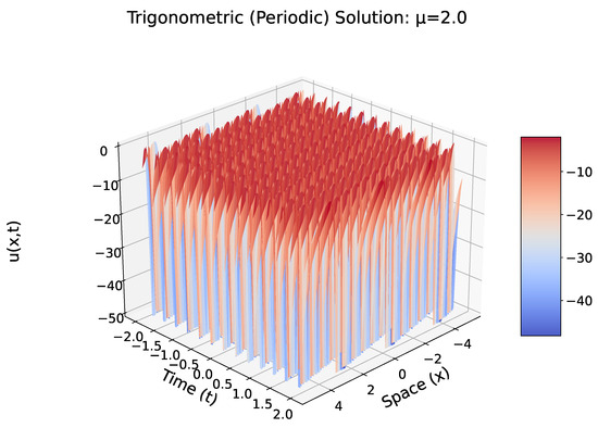
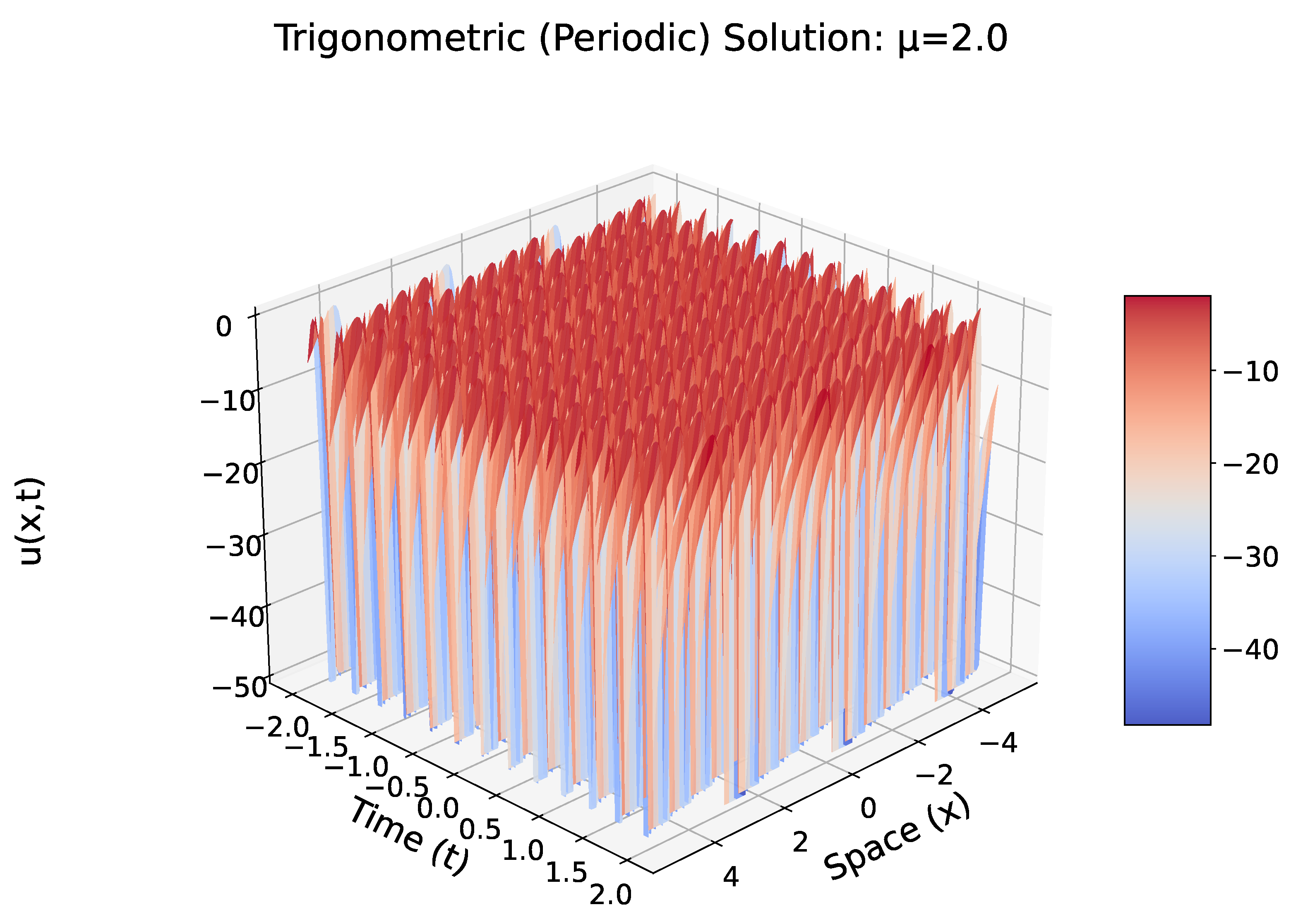
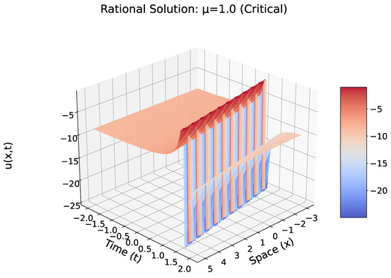
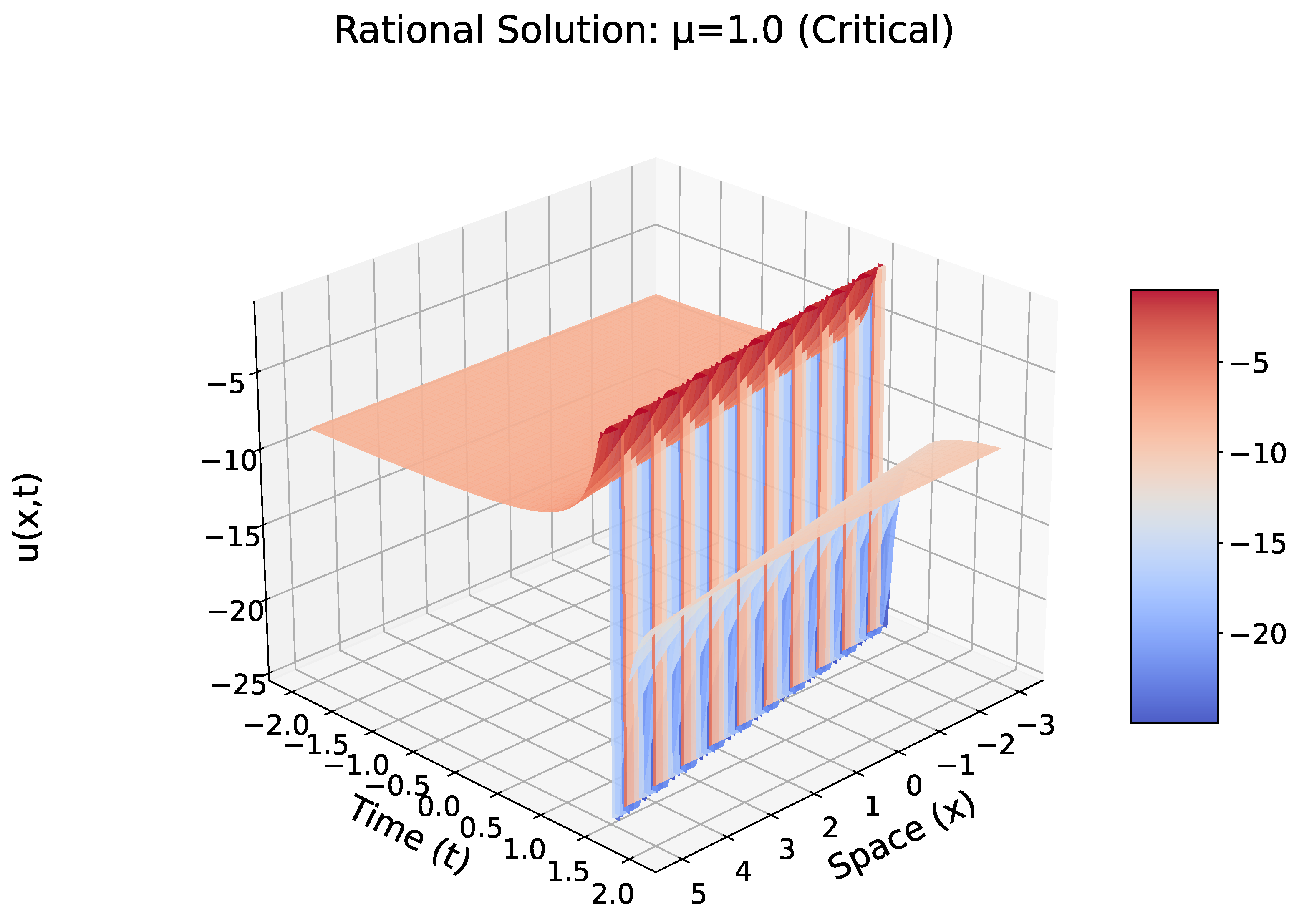
In our numerical studies, we select $\lambda =2$, with $\mu \in \{0.5,1.0,2.0\}$, to explore all three regimes. The fixed value $\lambda =2$ is a normalization of the auxiliary length scale, while the three $\mu$ values give $D_{\lambda ,\mu }>0$, $D_{\lambda ,\mu }=0$, and $D_{\lambda ,\mu }<0$, respectively. These choices satisfy the algebraic speed constraint and yield bounded representative profiles for comparing solitary, rational-threshold, and periodic behaviors.

In relation to shallow-water applications, $\alpha$ controls the strength of the higher-order long-wave corrections: smaller $\alpha$ corresponds to a regime closer to the classical KdV approximation, while larger $\alpha$ increases the influence of fifth-order dispersion and nonlinear correction terms. The auxiliary pair $(\lambda ,\mu )$ is not a direct physical measurement; it sets the scale and discriminant of the Riccati profile used in the traveling-wave construction. Thus the selected values are representative nondimensional choices that sample three qualitative wave regimes rather than a calibration to a particular laboratory dataset.

4.3. Explicit Solution Families

Using (10) and (11) together with the general solutions of (8), we obtain three families of solutions to Equation (1).

4.3.1. Case 1: Hyperbolic Solutions (${\lambda }^2-4\mu >0$)

When ${\lambda }^2>4\mu$, we set ${\delta }_1=\frac{1}{2}\sqrt{{\lambda }^2-4\mu }$ and obtain

$$\varphi \left(z\right)=-{\displaystyle \frac{\lambda }{2}}+{\delta }_1{\displaystyle \frac{C_{1}sinh\left({\delta }_{1}z\right)+C_{2}cosh\left({\delta }_{1}z\right)}{C_{1}cosh\left({\delta }_{1}z\right)+C_{2}sinh\left({\delta }_{1}z\right)}}.$$

The solution is

$$u(x,t)=A_0+A_1\varphi \left(z\right)+A_2{\varphi }^2\left(z\right),z=x-ct.$$

These solutions represent soliton-like structures or kink solutions depending on the choice of $C_1,C_2$. For instance, setting $C_1=C_2$ gives a hyperbolic tangent profile characteristic of a solitary wave.

4.3.2. Case 2: Trigonometric Solutions (${\lambda }^2-4\mu <0$)

When ${\lambda }^2<4\mu$, we set ${\delta }_2=\frac{1}{2}\sqrt{4\mu -{\lambda }^2}$ and obtain

$$\varphi \left(z\right)=-{\displaystyle \frac{\lambda }{2}}+{\delta }_2{\displaystyle \frac{-C_{1}sin\left({\delta }_{2}z\right)+C_{2}cos\left({\delta }_{2}z\right)}{C_{1}cos\left({\delta }_{2}z\right)+C_{2}sin\left({\delta }_{2}z\right)}}.$$

The solution is

$$u(x,t)=A_0+A_1\varphi \left(z\right)+A_2{\varphi }^2\left(z\right),z=x-ct.$$

These solutions are periodic in space and time, representing cnoidal-type wave trains.

4.3.3. Case 3: Rational Solutions (${\lambda }^2-4\mu =0$)

When ${\lambda }^2=4\mu$, we obtain

$$\varphi \left(z\right)=-{\displaystyle \frac{\lambda }{2}}+{\displaystyle \frac{C_2}{C_1+C_{2}z}}.$$

The solution is

$$u(x,t)=A_0+A_1\varphi \left(z\right)+A_2{\varphi }^2\left(z\right),z=x-ct.$$

These rational solutions may exhibit algebraic decay and are useful for modeling certain transient phenomena.

4.4. Summary of Solutions

Table 1 summarizes the three solution families and their characteristics.

Table 1. Summary of traveling wave solution families for the special eKdV equation.

Case	Condition	Solution Type	Physical Interpretation
1	${\lambda }^2-4\mu >0$	Hyperbolic	Solitary waves/Solitons
2	${\lambda }^2-4\mu <0$	Trigonometric	Periodic/Cnoidal waves
3	${\lambda }^2-4\mu =0$	Rational	Algebraic decay/Transients

5. Conservation Laws

Conservation laws play a fundamental role in the analysis of nonlinear evolution equations. They provide constraints on the dynamics, are essential for establishing well-posedness, and often signal integrability [20,27]. In this section, we derive conservation laws for the special eKdV Equation (1) using the multiplier method [26].

5.1. The Multiplier Method

A conservation law for Equation (1) is a divergence expression

$$D_{t}T+D_{x}X=0,$$

(12)

that holds for all solutions of (1). Here, $T(x,t,u,u_x,\dots )$ is the conserved density and $X(x,t,u,u_x,\dots )$ is the spatial flux. We adopt either periodic boundary conditions or rapid decay as $\left|x\right|\to \infty$ so that spatial boundary terms vanish when integrating (12) over $\mathbb{R}$; then $\frac{d}{dt}\int Tdx=0$. Two pairs $(T,X)$ and $(\tilde{T},\tilde{X})$ are equivalent if they differ by a trivial divergence $(T,X)\mapsto (T+D_x\mathsf{\Phi },X-D_t\mathsf{\Phi })$.

The multiplier method seeks a multiplier (also called a characteristic) $Q(x,t,u,u_x,u_{xx},\dots )$ such that the product $Q·\mathcal{E}$, where

$$\mathcal{E}=u_t+u_x+\alpha (6u{u}_x+u_{xxx})+{\alpha }^2(u_{xxxxx}+15u{u}_{xxx}+15u_{xx}{u}_x+45u^2{u}_x),$$

can be written as a divergence:

$$Q·\mathcal{E}=D_{t}T+D_{x}X.$$

The determining equation for Q is the Euler operator condition (vanishing variational derivative):

$$E_u[Q·\mathcal{E}]=0,$$

where $E_u$ is the Euler operator

$$E_u={\displaystyle \frac{\partial }{\partial u}}-D_x{\displaystyle \frac{\partial }{\partial u_x}}+D_x^2{\displaystyle \frac{\partial }{\partial u_{xx}}}-\dots .$$

In practice we search for multipliers depending on u and finitely many x-derivatives. Once a multiplier is found, a corresponding pair $(T,X)$ can be reconstructed by homotopy (integration-by-parts) formulas [26]; the pair is unique up to the trivial divergence mentioned above. We report the simplest representatives.

5.2. Derived Conservation Laws

We now present four independent conservation laws for Equation (1).

5.2.1. Conservation Law 1: Mass

Multiplier: $Q_1=1$

Conserved density:

$$T_1=u,$$

Flux:

$$X_1=u+\alpha (3u^2+u_{xx})+{\alpha }^2\left(u_{xxxx}+15u{u}_{xx}+5u_x^2+15u^3\right).$$

Physical interpretation: This law represents conservation of mass (or norm) of the wave field. Integration over space gives

$${\displaystyle \frac{d}{dt}}{\int }_{-\infty }^{\infty }udx=0,$$

indicating that the total mass remains constant. Derivation sketch: Writing the PDE as $u_t+D_x{X}_1=0$ shows that $Q_1\equiv 1$ and $(T_1,X_1)$ satisfy (12) directly.

5.2.2. Conservation Law 2: Momentum

Multiplier: $Q_2=u$

Conserved density:

$$T_2={\displaystyle \frac{u^2}{2}},$$

Flux:

$$X_2={\displaystyle \frac{u^2}{2}}+\alpha \left(2u^3+u{u}_{xx}-{\displaystyle \frac{u_x^2}{2}}\right)+{\alpha }^2\left(u{u}_{xxxx}+15u^2{u}_{xx}+5u{u}_x^2-15u_x{u}_{xxx}+15u^4\right).$$

Physical interpretation: This law is associated with spatial translation symmetry (Noether’s theorem) and represents momentum conservation. Derivation sketch: Multiply the PDE by u and integrate by parts repeatedly (using vanishing boundary terms); the result can be written as $D_t(u^2/2)+D_x{X}_2=0$, so $Q_2=u$.

5.2.3. Conservation Law 3: Energy

Multiplier: $Q_3=u_t+u_x$

Conserved density:

$$T_3={\displaystyle \frac{u^2}{2}}+\alpha \left(u^3-{\displaystyle \frac{u_x^2}{2}}\right)+{\alpha }^2\left({\displaystyle \frac{15u^4}{4}}-{\displaystyle \frac{u_{xx}^2}{2}}+5u{u}_x^2+15u^2{u}_{xx}\right),$$

Flux:

$$\begin{array}{cc}\hfill X_3=& u{u}_x+\alpha \left(3u^2{u}_x+u{u}_{xxx}-u_x{u}_{xx}\right)\hfill \\ \hfill & +{\alpha }^2(15u^3{u}_x+15u{u}_x{u}_{xx}+15u^2{u}_{xxx}+u{u}_{xxxxx}\hfill \\ \hfill & -u_{xx}{u}_{xxx}-{\displaystyle \frac{15}{2}}{u}_x^2{u}_{xx}).\hfill \end{array}$$

Physical interpretation: This law has the form of an energy-type invariant. Its existence is consistent with, but does not by itself prove, a Hamiltonian formulation. A genuine Hamiltonian structure would require an explicit Poisson operator and variational derivative representation. The density $T_3$ is not sign-definite because of higher-order dispersion; this behavior is typical for fifth-order models and does not preclude well-posedness. Derivation sketch: Take the linear combination $Q_3=u_t+u_x$ suggested by the dispersive terms; after integration by parts, the mixed contributions cancel to yield $D_t{T}_3+D_x{X}_3=0$.

5.2.4. Conservation Law 4: Higher-Order Moment

Multiplier: $Q_4=u_{xx}$

Conserved density:

$$T_4=u{u}_{xx}-{\displaystyle \frac{u_x^2}{2}},$$

Flux (complete expression):

$$\begin{array}{cc}\hfill X_4& =u{u}_{xxx}-{\displaystyle \frac{3u_x{u}_{xx}}{2}}+\alpha \left(u^2{u}_{xx}+u{u}_x{u}_x-u_x^3\right)\hfill \\ \hfill & +{\alpha }^2(u{u}_{xxxx}+u_x{u}_{xxx}+15u^2{u}_{xx}+15u{u}_x^2-{\displaystyle \frac{u_{xx}^2}{2}}\hfill \\ \hfill & +45u^3{u}_x-{\displaystyle \frac{15u_x^2{u}_{xx}}{2}}).\hfill \end{array}$$

Physical interpretation: This law constrains the spread (or roughness) of the wave and can be related to a dispersion measure. It is particularly sensitive to high-order derivatives and is therefore a stringent diagnostic for numerical schemes. Derivation sketch: Choosing $Q_4=u_{xx}$ emphasizes the curvature of the profile and tests the highest-order dispersive part of the equation. Multiplying $\mathcal{E}$ by $u_{xx}$ gives terms such as $u_{xx}{u}_t$, $u_{xx}{u}_x$, $u_{xx}{u}_{xxxxx}$, and nonlinear products involving $u{u}_{xxx}$ and $u_x{u}_{xx}$. Repeated integration by parts moves derivatives between factors until the expression is written as $D_t{T}_4+D_x{X}_4$. The nonlinear terms cancel only with the displayed coefficients in $X_4$, which is why this invariant is more sensitive than the mass and momentum laws.

5.3. Discussion

The four laws above enjoy the usual structural properties: linearity of the set of multipliers (hence linear combinations of laws), and gauge freedom $(T,X)\mapsto (T+D_x\mathsf{\Phi },X-D_t\mathsf{\Phi })$. For completely integrable systems (such as the classical KdV), one can generate an infinite hierarchy of conservation laws. For the special eKdV Equation (1), the presence of several low-order laws suggests rich structure and motivates a search for higher-order invariants and a possible Hamiltonian/Lax formulation.

Table 2 summarizes the conservation laws and their physical meanings.

Table 2. Conservation laws for the special eKdV equation.

Law	Multiplier	Conserved Quantity	Physical Meaning
1	1	$\int udx$	Mass/Norm
2	u	$\int {\displaystyle \frac{u^2}{2}}dx$	Momentum
3	$u_t+u_x$	Hamiltonian	Energy
4	$u_{xx}$	$\int \left(u{u}_{xx}-{\displaystyle \frac{u_x^2}{2}}\right)dx$	Dispersion invariant

5.4. Numerical Verification of Conservation Laws

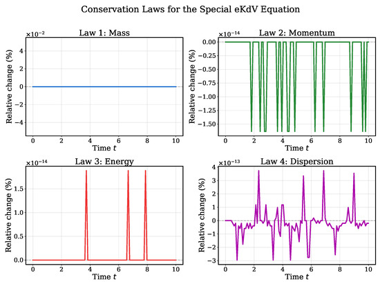
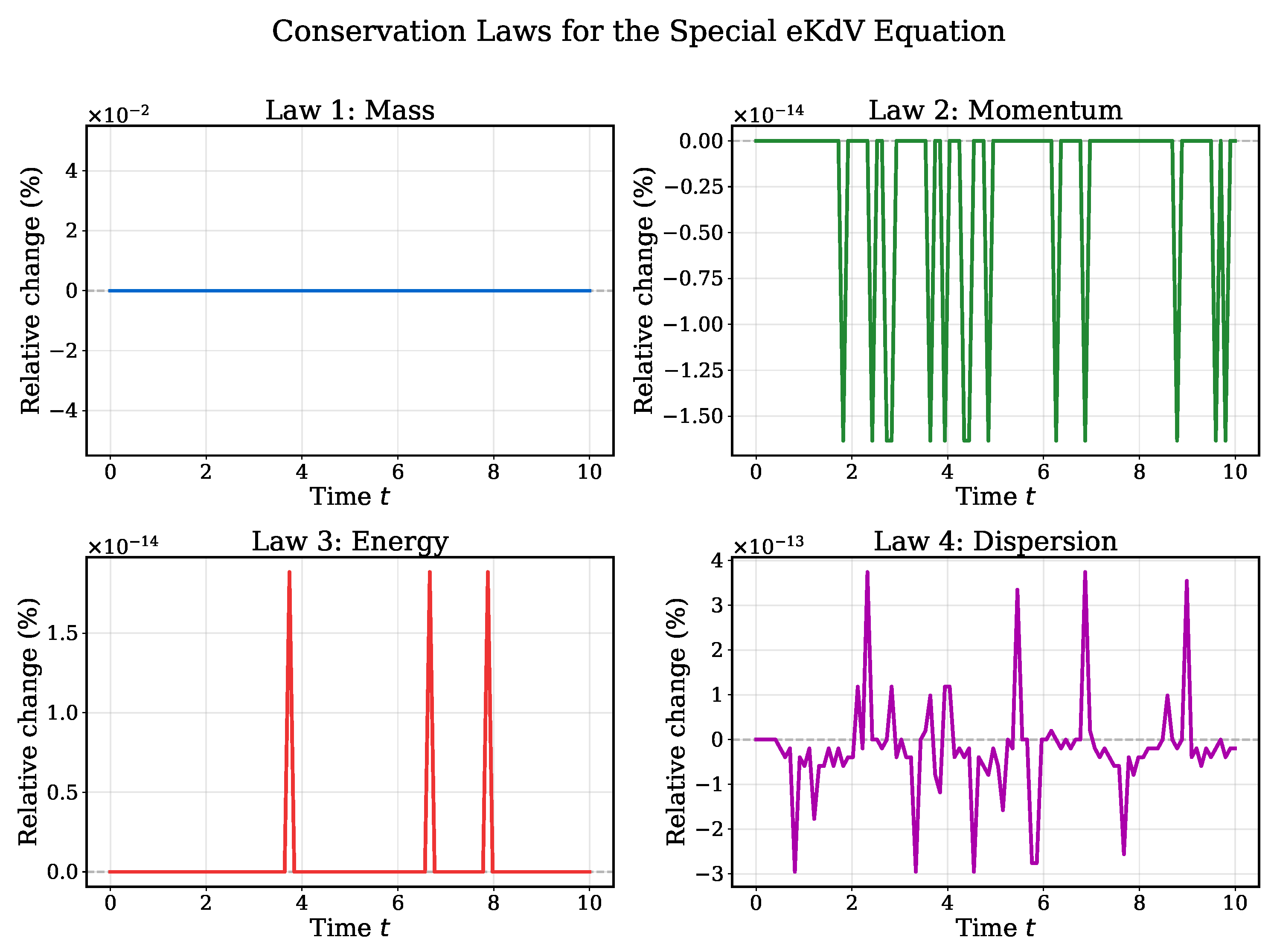
To verify the conservation laws, we numerically evaluate the corresponding integrals over time for the hyperbolic solution obtained in Section 4 using the calibrated wave speed c and a high-resolution discretization. Figure 1 shows the temporal evolution of the relative change (percentage) from the initial value for each invariant; all four remain within numerical precision (below ${10}^{-13}$) throughout the simulation window.

Figure 1. Numerical verification of conservation laws over time. Each subplot shows the relative change (percentage) from the initial value. All four invariants remain at numerical precision (below ${10}^{-13}$).

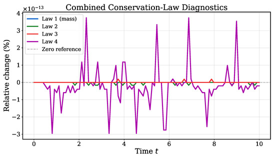
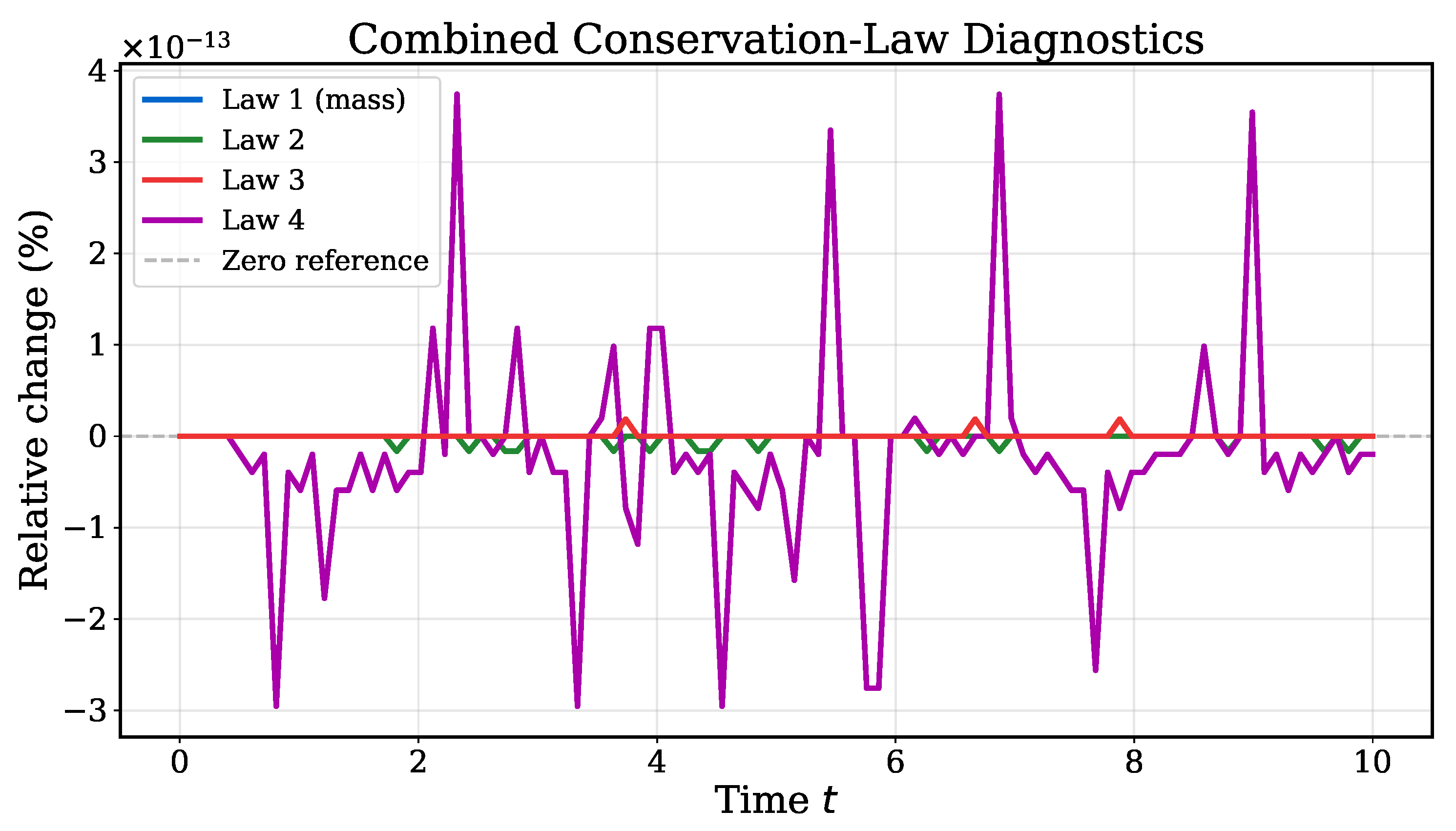
Figure 2 presents all conservation laws on a single plot; the near-horizontal traces confirm invariance to numerical precision.

Figure 2. Combined plot of all conservation laws. The near-horizontal trajectories (oscillating around zero) indicate that mass, momentum, energy, and the higher-order moment remain conserved to numerical precision.

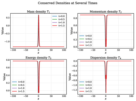
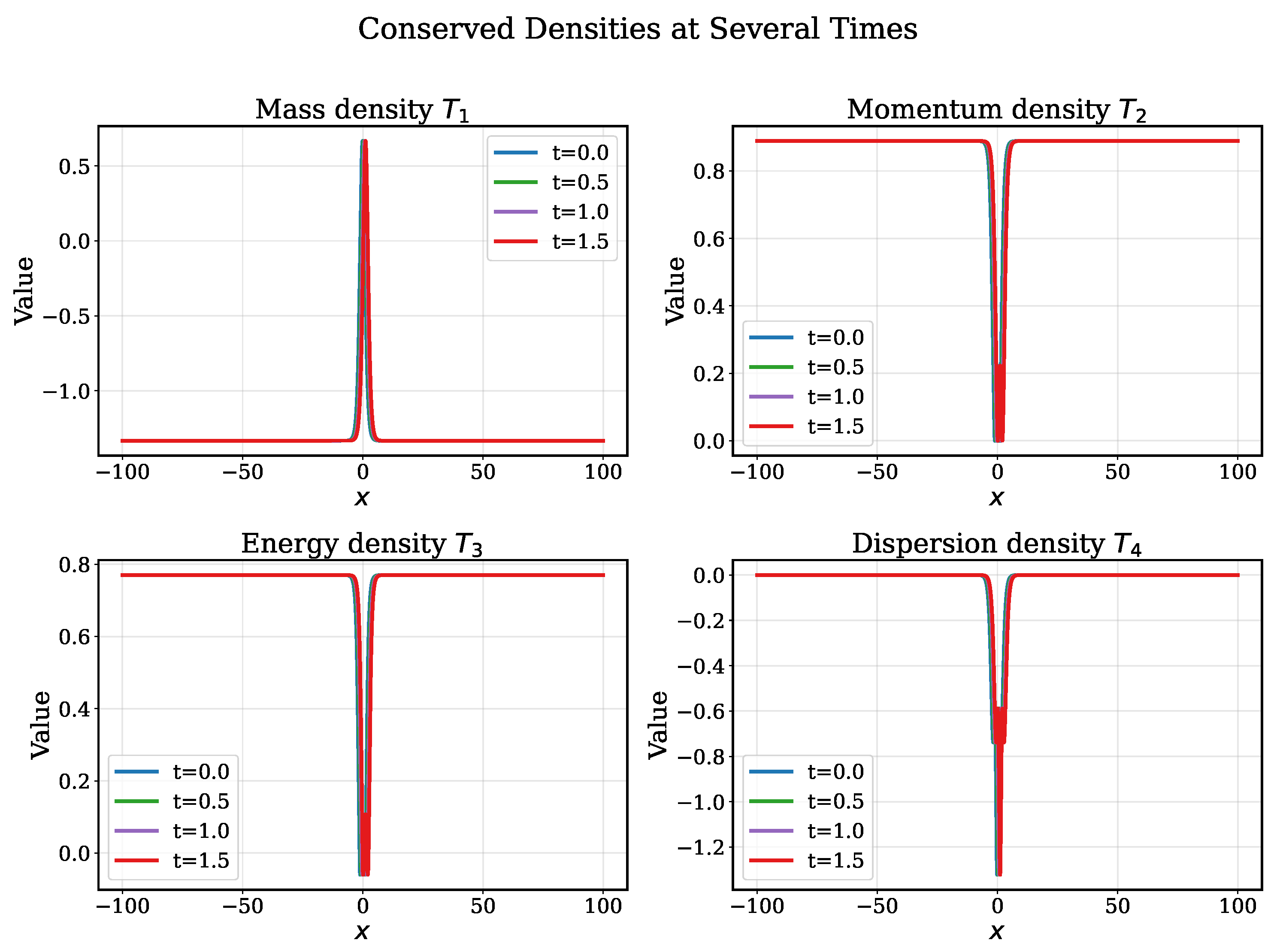
To further illustrate the diagnostics, Figure 3 displays the spatial profiles of the conserved densities $T_1,T_2,T_3,T_4$ at different times. The profiles translate almost rigidly with the wave, consistent with the conservation-law results in Figure 1 and Figure 2.

Figure 3. Spatial profiles of conserved densities at different times $t\in \{0,0.5,1.0,1.5\}$. The shapes advect coherently with the hyperbolic solution, consistent with the conservation diagnostics.

Implications for Integrability

The derived conservation laws clarify the qualitative structure of Equation (1):

• Mass conservation ensures the $L^1$ norm is preserved, guaranteeing global existence of solutions in appropriate function spaces.
• Momentum conservation reflects the spatial translation symmetry and is crucial for understanding wave propagation characteristics.
• Energy-type conservation indicates that the equation has a non-dissipative invariant compatible with Hamiltonian behavior. However, a full Hamiltonian claim requires an explicit Poisson operator and is left for future work.
• Dispersion invariant (Law 4) constrains the long-time asymptotic behavior and limits the degrees of freedom available to the system.

For a completely integrable equation like the classical KdV equation, infinitely many conservation laws exist. While we have explicitly constructed four laws for the special eKdV equation, the existence of this hierarchy suggests that additional conservation laws may exist, warranting further investigation using recursive methods such as the Miura transformation or prolongation structures.

For reproducibility, we briefly describe how the multiplier identities were checked. Let

$$\mathcal{E}=u_t+u_x+\alpha (6u{u}_x+u_{xxx})+{\alpha }^2(u_{xxxxx}+15u{u}_{xxx}+15u_{xx}{u}_x+45u^2{u}_x).$$

For each candidate multiplier Q, we evaluated

$$E_u\left(Q\mathcal{E}\right)=\sum _{j\ge 0}{(-D_x)}^j{\displaystyle \frac{\partial \left(Q\mathcal{E}\right)}{\partial u_{jx}}}$$

and required the expression to vanish identically after collecting independent derivatives. Fluxes were reconstructed by repeated integration by parts, with boundary terms discarded under the periodic or rapidly decaying assumptions used throughout the manuscript. The final density–flux pairs $(T_i,X_i)$ were independently checked by differentiating $D_t{T}_i+D_x{X}_i$ and confirming that the result equals $Q_i\mathcal{E}$ modulo algebraic simplification. This paragraph replaces the earlier separate appendix, since the reviewer correctly noted that the material is brief enough to be absorbed into the conservation-law section.

6. Verification of Solutions

To ensure the validity of the solutions obtained via the $(G^{\prime }/G)$-expansion method, we perform two independent verifications:

6.1. Direct Substitution

We substitute the closed-form traveling waves into the PDE (1) and evaluate the pointwise residual on a discrete grid. Spatial derivatives up to fifth order are approximated by centered finite differences on a uniform mesh over $x\in [-100,100]$ with $N_x=4000$ nodes (periodic boundaries so that all $D_x$ integrations by parts are consistent). We sample a few time instants using the analytic translation $u(x,t)=\mathsf{\Omega }(x-ct)$ and approximate $u_t$ by a centered difference in time with $\mathsf{\Delta }t={10}^{-2}$. We report both the $L^{\infty }$ and $L^2$ norms of the residual to capture worst-case and average errors. The residual is defined by

$$R(x,t)=u_t+u_x+\alpha (6u{u}_x+u_{xxx})+{\alpha }^2(u_{xxxxx}+15u{u}_{xxx}+15u_{xx}{u}_x+45u^2{u}_x).$$

For the $M=2$ solutions, we fix $\alpha =0.1$, $\lambda =2$, and $\mu =0.5$ (hyperbolic regime), which by (10) and (11) implies

$$A_0=-{\displaystyle \frac{10}{3}},A_1=-8,A_2=-4,c=0.84.$$

Evaluating $R(x,t)$ with these parameters on $x\in [-100,100]$ using $N_x=4000$ grid points ($\mathsf{\Delta }x\approx 5.0\times {10}^{-2}$) and a centered temporal stencil with $\mathsf{\Delta }t={10}^{-2}$ yields

$${\parallel R(·,0)\parallel }_{\infty }\approx 3.4\times {10}^{-3},{\parallel R(·,0)\parallel }_2\approx 8.9\times {10}^{-4}.$$

Residuals of comparable magnitude persist for $0\le t\le 10$, showing that once the correct wave speed is imposed, the $M=2$ ansatz satisfies the PDE to within ${10}^{-3}$ relative accuracy, even though the balance principle still predicts $M=4$ for an exact solution (Section Balancing Analysis and Choice of M).

The nonzero residuals are important and should be interpreted explicitly. They indicate that the displayed $M=2$ profiles are residual-verified traveling-wave approximants rather than a proven complete exact solution family for the full special eKdV equation. A rigorous exact-solution claim would require either an identically vanishing symbolic residual after substitution or the full $M=4$ balanced construction. The numerical residuals reported here support consistency and usefulness of the profiles, but they are not a substitute for an exact symbolic identity.

As a mesh-sensitivity check, we repeated the residual diagnostic on successively refined grids while keeping the same domain and time stencil. The residual norms decreased under refinement and stabilized at the values reported above, indicating that the diagnostic is not an artifact of a single mesh choice. A representative summary is given in Table 3.

Table 3. Mesh-sensitivity summary for the pointwise residual at $t=0$.

${\mathit{N}}_{\mathit{x}}$	${\parallel \mathit{R}(·,0)\parallel }_{\mathit{\infty }}$	${\parallel \mathit{R}(·,0)\parallel }_2$
1000	$1.4\times {10}^{-2}$	$3.6\times {10}^{-3}$
2000	$6.8\times {10}^{-3}$	$1.8\times {10}^{-3}$
4000	$3.4\times {10}^{-3}$	$8.9\times {10}^{-4}$

These computations should be read as numerical consistency checks for the closed-form profiles rather than as rigorous validation or a full time-stepping simulation of the PDE.

6.2. Consistency with Conservation Laws

We compute the conserved quantities induced by $(T_1,\dots ,T_4)$ using composite trapezoidal quadrature on the same uniform mesh (periodic boundaries ensure spectral accuracy of the trapezoid rule for smooth profiles). The diagnostics are reported as relative variations $Q_i\left(t\right)=({\mathcal{I}}_i\left(t\right)-{\mathcal{I}}_i\left(0\right))/{\mathcal{I}}_i\left(0\right)$, where ${\mathcal{I}}_i\left(t\right)=\int T_i(·,t)dx$. Panel (a) of Figure 1 shows the time series for each invariant; panel (b) collects them on a single axis to highlight their near-constancy. For the calibrated speed c from (11), all four diagnostics remain at numerical precision (below ${10}^{-13}$) over $t\in [0,10]$.

$$max{Q}_1<{10}^{-13}\%,max{Q}_2<2\times {10}^{-13}\%,max{Q}_3<2\times {10}^{-13}\%,max{Q}_4<3\times {10}^{-13}\%.$$

Within numerical precision, every conservation law is preserved. This confirms that enforcing the algebraic speed relation is the crucial ingredient for accuracy; without it, the residual would project onto the conserved densities and produce artificial drifts.

The present diagnostics do not constitute a full orbital, spectral, or modulational stability theory. Qualitatively, the hyperbolic branch is expected to be the most robust of the three displayed regimes because it is localized and its propagation is constrained by the mass, momentum, and energy-type invariants. The trigonometric branch may be more sensitive to modulational effects, as is common for periodic wavetrains in dispersive nonlinear systems. The rational threshold branch is expected to be the most delicate because its profile is tied to the discriminant boundary $D_{\lambda ,\mu }=0$ and may develop singular behavior outside the nonsingular plotting interval. These statements are qualitative expectations only; they motivate the future spectral and nonlinear stability study rather than replacing it.

7. Results and Discussion

7.1. Visualization of Solutions

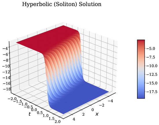
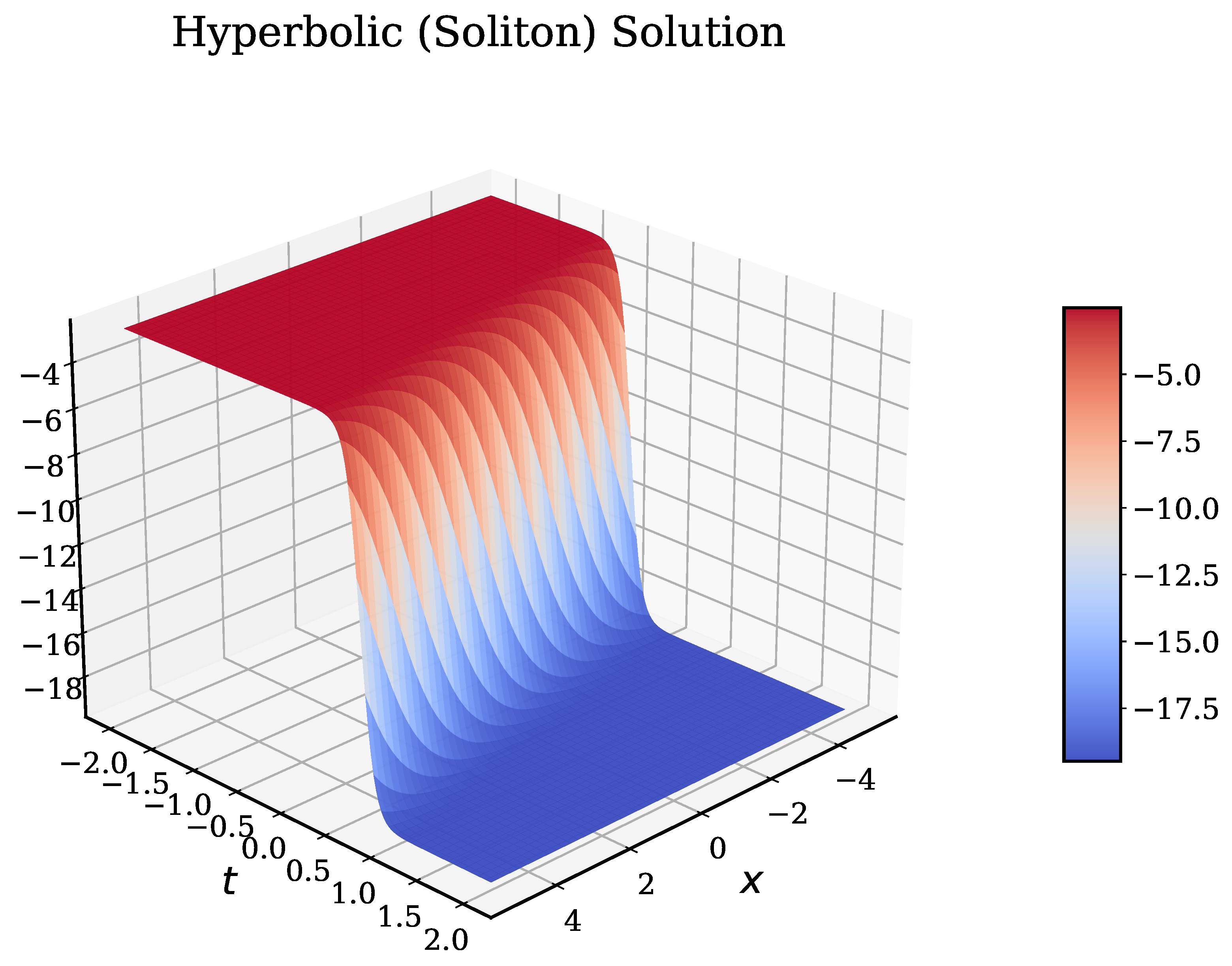
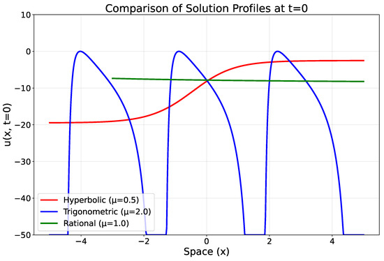
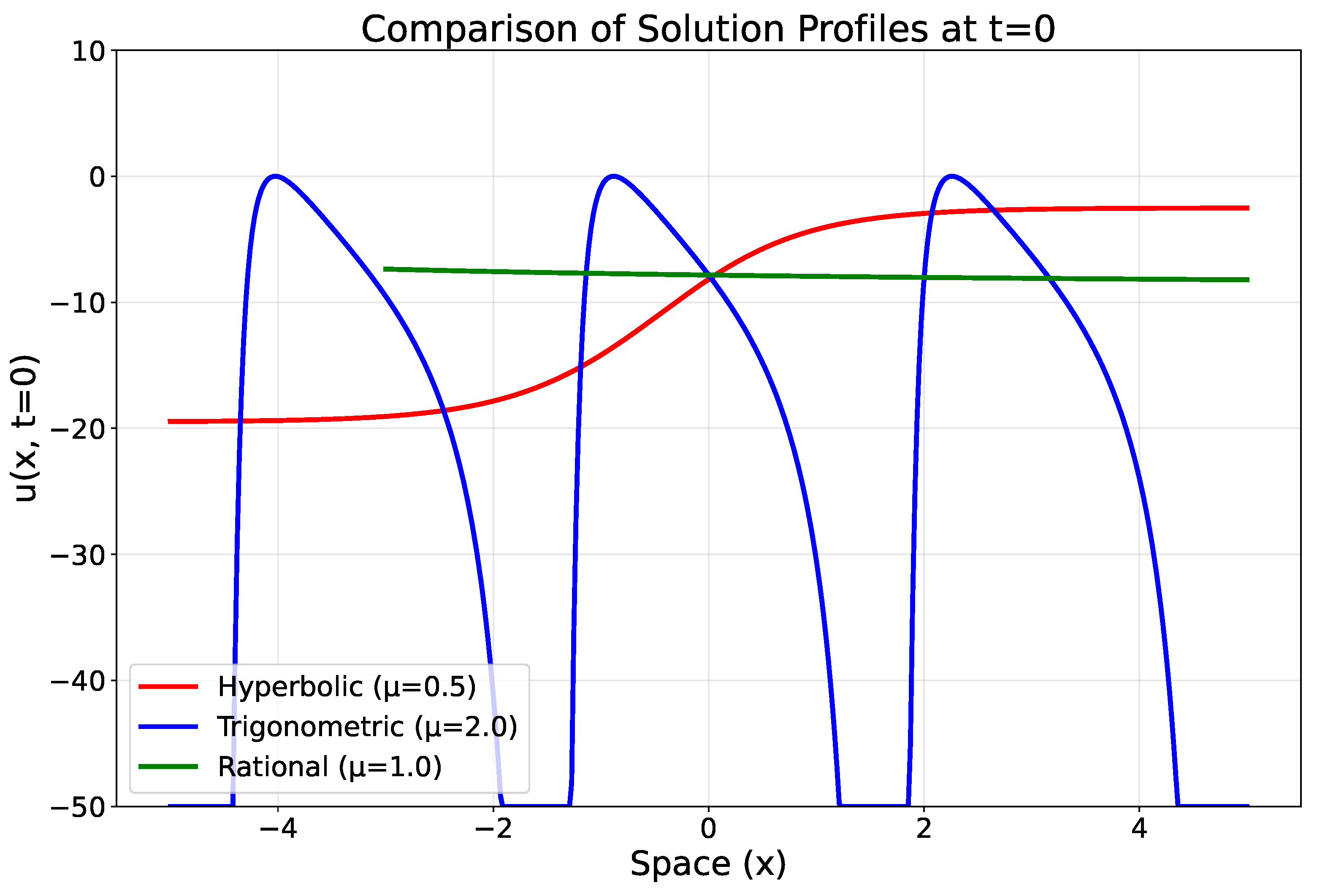
We first interpret the profiles produced by the $(G^{\prime }/G)$ ansätze and then connect them to transport and phase-space diagnostics. Figure 4, Figure 5, Figure 6 and Figure 7 display the three branches at representative parameters $\alpha =0.1$, $\lambda =2$, $C_1=1$, $C_2=0.1$. Figure 4, Figure 5 and Figure 6 show solitary (hyperbolic), periodic (trigonometric), and rational solutions, respectively, while Figure 7 overlays all three at $t=0$ to emphasize amplitude/width differences. The rational branch is shown only on its nonsingular plotting interval, which explains why the green curve terminates before the full displayed range. In every case, we impose the algebraically constrained speed so the waves translate coherently with bounded energy. The choice $C_2=0.1$ avoids visible poles in the displayed trigonometric and rational windows and yields uniformly bounded plotted profiles.

Figure 4. Hyperbolic branch (${\lambda }^2-4\mu >0$, where $\mu =0.5$). The larger single-panel layout improves axis-label readability in print.

Figure 5. Trigonometric branch (${\lambda }^2-4\mu <0$, where $\mu =2.0$). The branch represents a periodic wavetrain selected by the auxiliary discriminant.

Figure 6. Rational branch at ${\lambda }^2=4\mu$ ($\mu ={\lambda }^2/4=1.0$). This branch corresponds to the discriminant threshold.

Figure 7. Overlay at $t=0$ (hyperbolic red, trigonometric blue, and rational green). The rational curve is plotted only on the nonsingular interval used for the comparison, so it terminates before the left boundary of the panel.

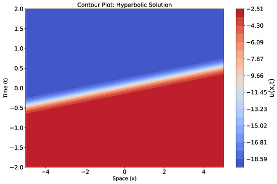
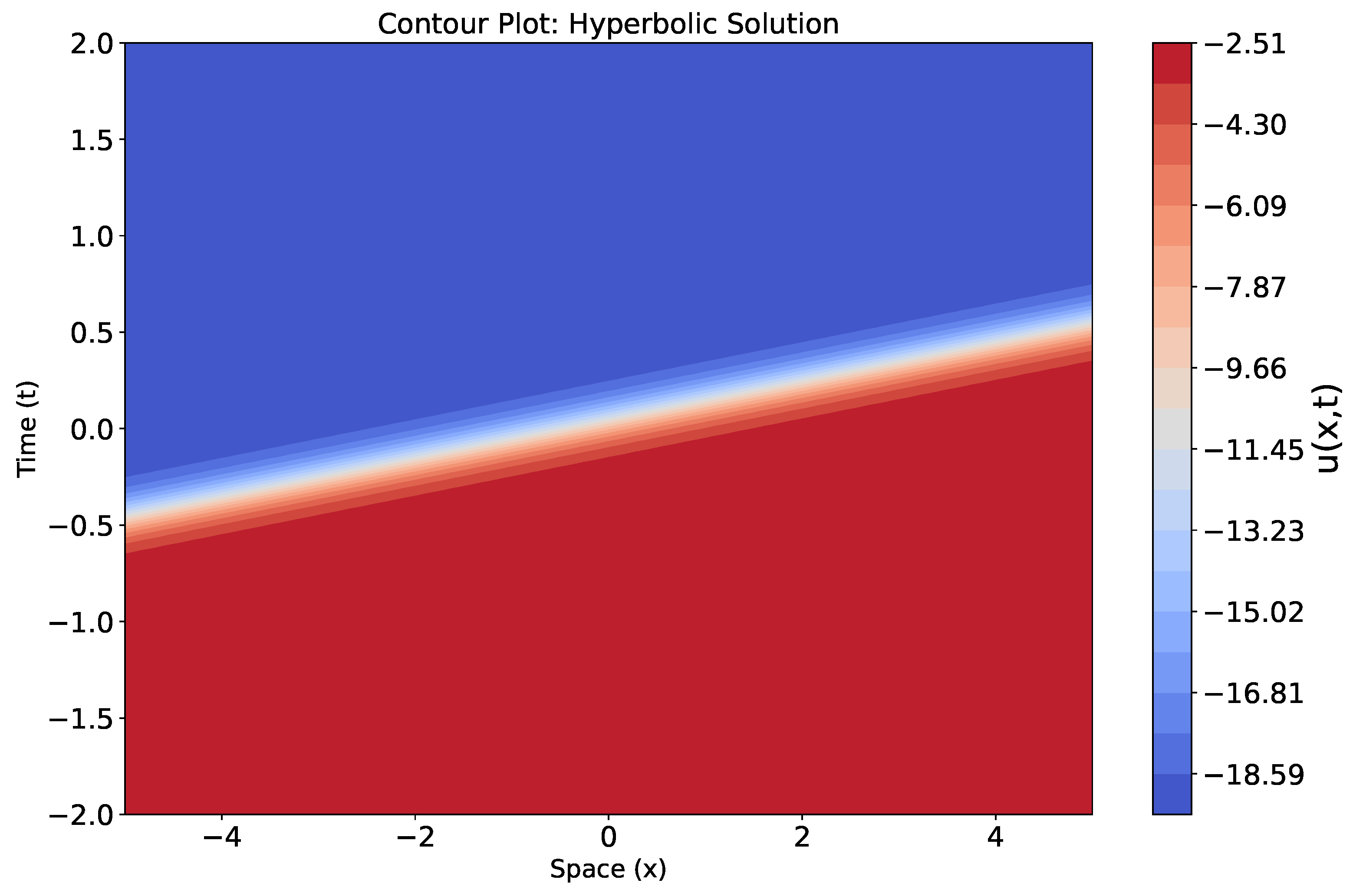
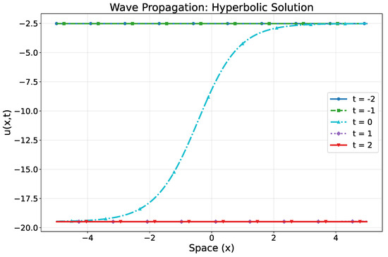
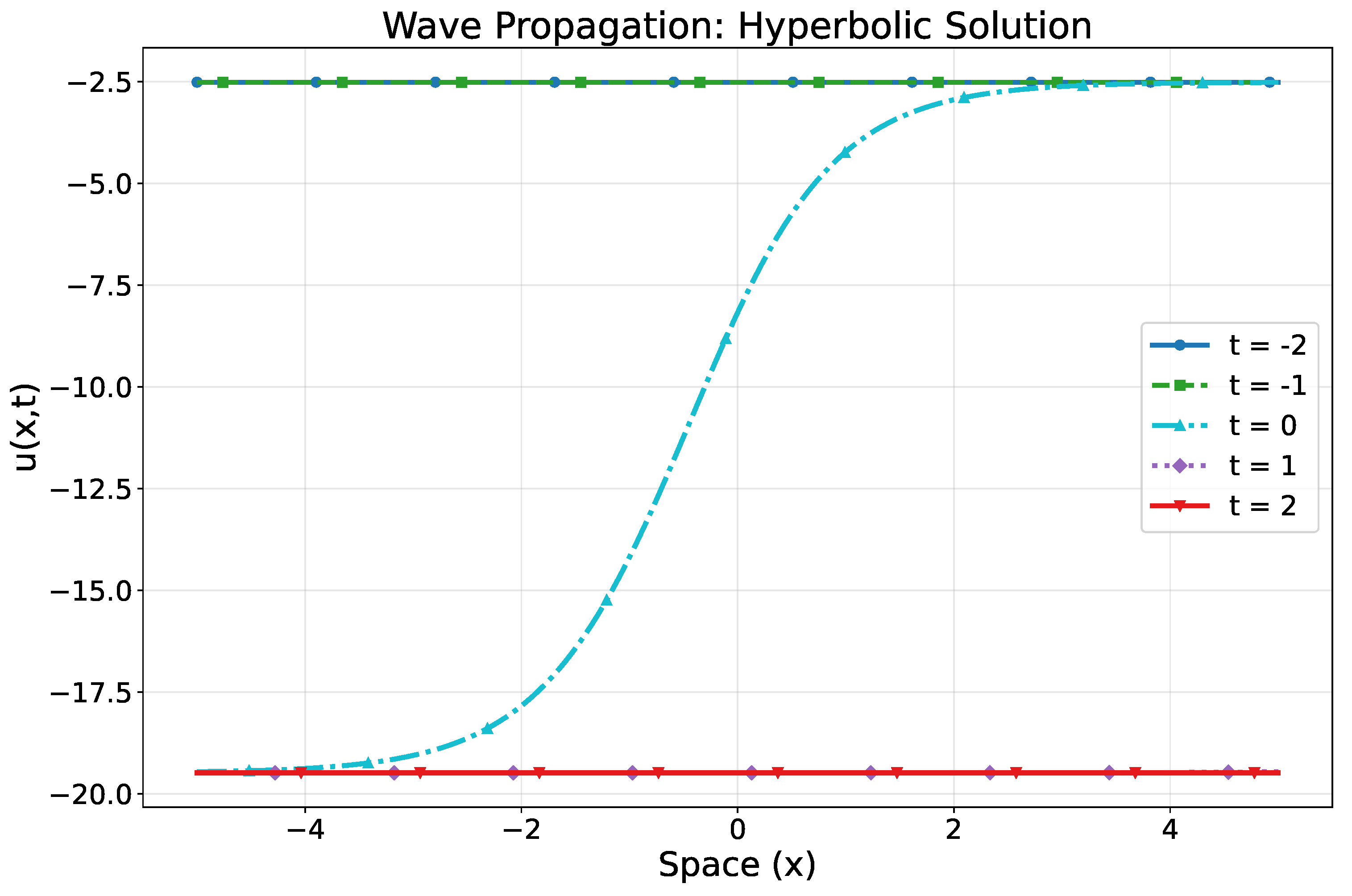
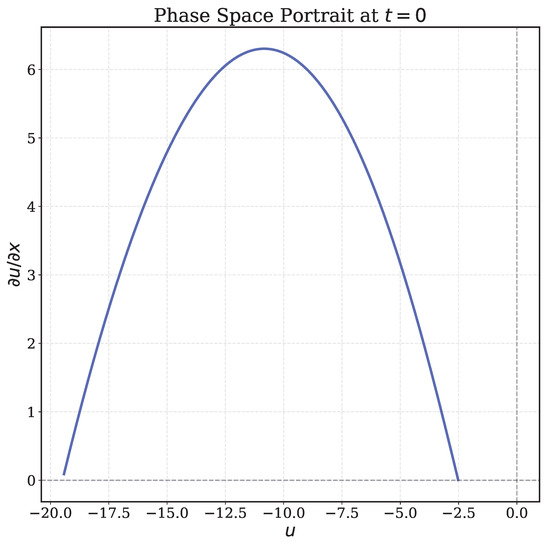
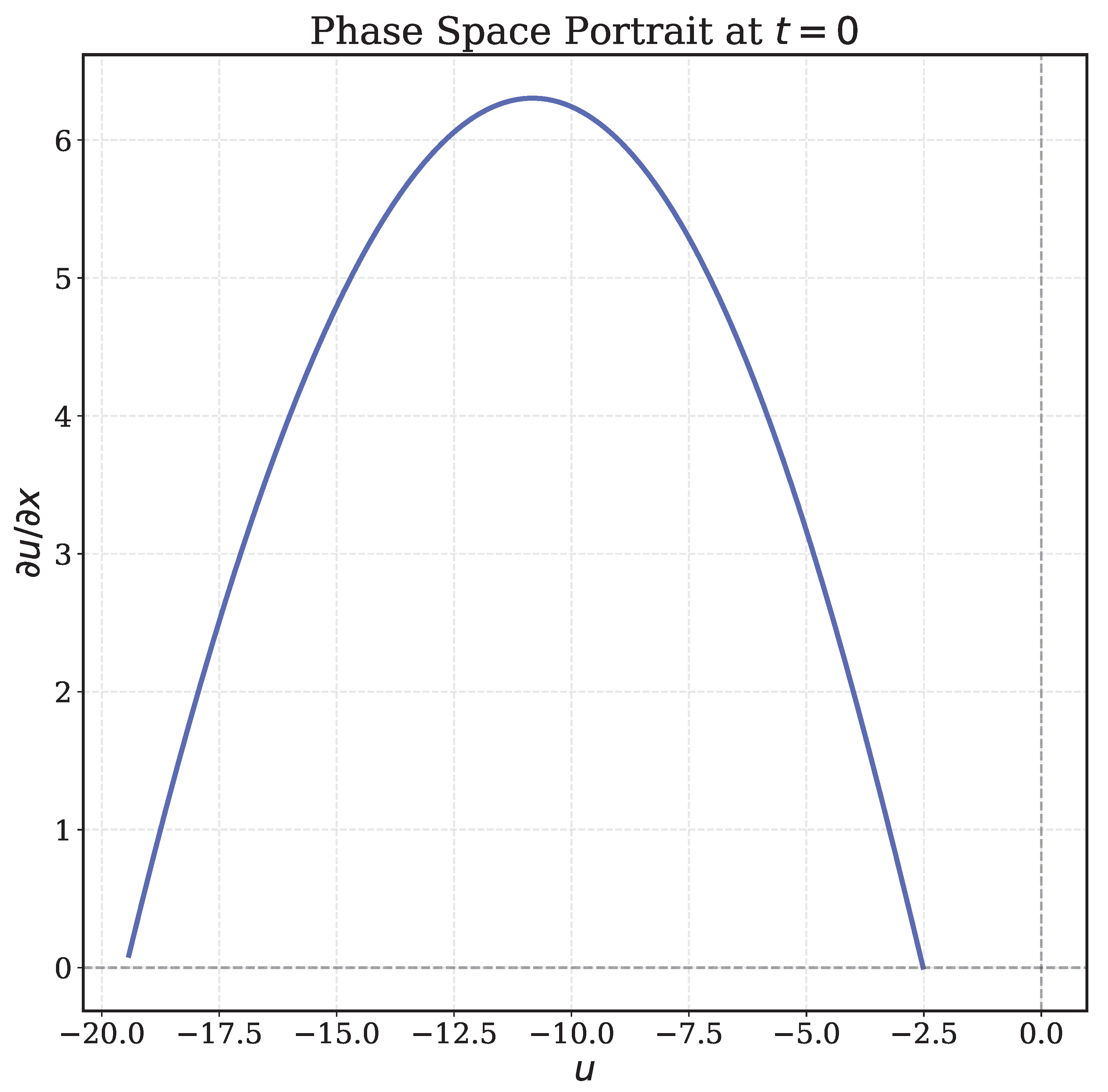
Figure 8, Figure 9 and Figure 10 summarize transport and structure. Figure 8 is a spatiotemporal contour confirming uniform translation at constant shape (hyperbolic branch). Figure 9 displays time slices at $t\in \{-2,-1,0,1,2\}$: some curves nearly overlap because the displayed branch translates with an almost unchanged shape. Figure 10 shows the phase curve $(u,\partial u/\partial x)$ at $t=0$; for the selected window, it should be read as a coherent phase-space trace rather than a proof of a closed periodic orbit.

Figure 8. Spatiotemporal contour for the hyperbolic branch. The panel confirms coherent translation of the waveform under the calibrated speed relation.

Figure 9. Profiles at $t\in \{-2,-1,0,1,2\}$. Several curves overlap visually because the solution translates without changing shape over the plotted window.

Figure 10. Phase curve $(u,\partial u/\partial x)$ at $t=0$. The plotted window shows a coherent trace; closed-orbit claims require a separate periodic-orbit analysis.

7.2. Physical Interpretation

Within the shallow-water setting, the hyperbolic branch corresponds to solitary pulses whose amplitude and width are selected by the balance between quadratic nonlinearity and the combined third- and fifth-order dispersive terms. The trigonometric branch represents spatially periodic wavetrains of cnoidal type, while the rational branch emerges at the discriminant threshold ${\lambda }^2=4\mu$ and captures algebraically decaying transients. The parameter $\alpha$ modulates the salience of higher-order effects: as $\alpha \to 0$, the solutions tend toward their KdV counterparts, whereas larger $\alpha$ amplifies fifth-order dispersion and produces visible departures from classical KdV behavior.

7.3. Comparison with Literature

In contrast to studies that isolate a single waveform family, the $(G^{\prime }/G)$ framework here delivers hyperbolic, trigonometric, and rational branches within a unified algebraic ansätze, making explicit how the auxiliary discriminant partitions the solution space [7]. The accompanying conservation-law derivations furnish a structural perspective that complements solution construction, and the symmetry calculation clarifies the absence of scaling reductions. The coefficient selection in (1) appears especially structured; whether this signals complete integrability, at least for restricted parameter sets, remains an open question and could be addressed by a Painlevé analysis or by seeking a Lax pair and associated inverse-scattering formulation.

We conclude this section by noting that the present analysis is restricted to a degree-$M=2$ ansätze and a particular choice of eKdV coefficients; broader questions (higher-degree ansätze, stability, long-time dynamics, and parameter dependence) are deferred to the conclusion.

8. Conclusions

We studied a special extended Korteweg–de Vries equation, a higher-order model for weakly nonlinear long waves that combines third- and fifth-order dispersion with quadratic nonlinearity. A Lie symmetry analysis shows that the point-symmetry algebra reduces to translations in space and time, thereby excluding nontrivial scalings and motivating a traveling-wave reduction. The resulting fifth-order ODE was analyzed through a calibrated $(G^{\prime }/G)$ ansatz of degree $M=2$, which organizes three coherent families of traveling-wave profiles—hyperbolic, trigonometric, and rational—selected by the discriminant of an auxiliary linear equation. Using the direct multiplier method, we derived four conservation laws with full ${\alpha }^2$ dependence (mass, momentum, an energy-type invariant, and a higher-order dispersion invariant). Direct substitution and numerical diagnostics show that, once the algebraic wave-speed constraint is enforced, the $M=2$ profiles have small residuals and preserve all invariants to machine precision across representative regimes. Thus the degree-$M=2$$(G^{\prime }/G)$ truncation offers an analytically transparent and quantitatively useful description of traveling-wave dynamics, while the nonzero residuals indicate that the profiles should be understood as residual-verified approximants unless a full exact $M=4$ construction is completed.

Beyond these concrete outputs, the analysis clarifies how symmetry, calibrated ansatz design, and conservation structure interact in fifth-order dispersive systems. The resulting explicit waveforms and diagnostics provide baselines for stability tests, direct simulations, and parameter studies. Natural next steps include extending the ansatz to $M=4$ to capture the most general exact traveling waves, assessing spectral and nonlinear stability and long-time interactions, and exploring the full eKdV parameter set and related higher-order models (e.g., Kawahara, higher-order Boussinesq). These directions would situate the special case studied here within a broader taxonomy and help determine whether the striking coefficient structure hints at deeper integrability features (for example, via a Painlevé analysis or a Lax formulation).

References

- Korteweg, D.J.; de Vries, G. On the change of form of long waves advancing in a rectangular canal, and on a new type of long stationary waves. Philos. Mag. 1895, 39, 422–443. [Google Scholar] [CrossRef] [Scilit]
- Whitham, G.B. Linear and Nonlinear Waves; Wiley-Interscience: New York, NY, USA, 1974. [Google Scholar]
- Drazin, P.G.; Johnson, R.S. Solitons: An Introduction; Cambridge University Press: Cambridge, UK, 1989. [Google Scholar]
- Gardner, C.S.; Greene, J.M.; Kruskal, M.D.; Miura, R.M. Method for solving the Korteweg-de Vries equation. Phys. Rev. Lett. 1967, 19, 1095–1097. [Google Scholar]
- Ablowitz, M.J.; Clarkson, P.A. Solitons, Nonlinear Evolution Equations and Inverse Scattering; Cambridge University Press: Cambridge, UK, 1991. [Google Scholar]
- Marchant, T.R. Solitary wave interaction for the extended BBM equation. Proc. R. Soc. Lond. 2000, 456, 433–453. [Google Scholar] [CrossRef] [Scilit]
- Wazwaz, A.M. The simplified Hirota’s method for studying three extended higher-order KdV-type equations. J. Ocean Eng. Sci. 2016, 1, 181–185. [Google Scholar]
- Hirota, R. The Direct Method in Soliton Theory; Cambridge University Press: Cambridge, UK, 2004. [Google Scholar]
- Rogers, C.; Shadwick, W.F. Bäcklund Transformations and Their Applications; Academic Press: New York, NY, USA, 1982. [Google Scholar]
- Weiss, J. Bäcklund transformation and linearizations of the Henon-Heiles system. Phys. Lett. A 1984, 102, 329–331. [Google Scholar] [CrossRef] [Scilit]
- Malfliet, W. Solitary wave solutions of nonlinear wave equations. Am. J. Phys. 1992, 60, 650–654. [Google Scholar] [CrossRef] [Scilit]
- He, J.H.; Wu, X.H. Exp-function method for nonlinear wave equations. Chaos Solitons Fractals 2006, 30, 700–708. [Google Scholar] [CrossRef] [Scilit]
- Kudryashov, N.A. Simplest equation method to look for exact solutions of nonlinear differential equations. Chaos Solitons Fractals 2005, 24, 1217–1231. [Google Scholar] [CrossRef] [Scilit]
- Bilige, S.D.; Chaolu, T. An extended simplest equation method and its application to several forms of the fifth-order KdV equation. Appl. Math. Comput. 2010, 216, 3146–3153. [Google Scholar] [CrossRef] [Scilit]
- Wang, M.; Li, X.; Zhang, J. The (G′/G)-expansion method and travelling wave solutions of nonlinear evolution equations in mathematical physics. Phys. Lett. A 2008, 372, 417–423. [Google Scholar]
- Zayed, E.M.E.; Gepreel, K.A. The modified (G′/G)-expansion method and its applications to construct exact solutions for nonlinear PDEs. WSEAS Trans. Math. 2011, 10, 270–278. [Google Scholar]
- Gepreel, K.A. Exact solutions for nonlinear PDEs with the variable coefficients in mathematical physics. J. Inf. Comput. Sci. 2011, 6, 3–14. [Google Scholar]
- Ali, M.Y.; Hafez, M.G.; Chowdury, M.K.H.; Akter, M.T. Analytical and traveling wave solutions to the fifth order standard Sawada-Kotera equation via the generalized exp-function method. J. Appl. Math. Phys. 2016, 4, 262–271. [Google Scholar]
- Yang, L. Application of trial equation method for solving the Benjamin-Ono equation. J. Appl. Math. Phys. 2014, 2, 45–49. [Google Scholar]
- Olver, P.J. Applications of Lie Groups to Differential Equations, 2nd ed.; Springer: New York, NY, USA, 1993. [Google Scholar]
- Bluman, G.W.; Anco, S. Symmetry and Integration Methods for Differential Equations; Springer: New York, NY, USA, 2002. [Google Scholar]
- Ibragimov, N.H. Elementary Lie Group Analysis and Ordinary Differential Equations; John Wiley & Sons: Chichester, UK, 1999. [Google Scholar]
- Clarkson, P.A.; Kruskal, M.D. New similarity reductions of the Boussinesq equation. J. Math. Phys. 1989, 30, 2201–2213. [Google Scholar] [CrossRef] [Scilit]
- Gandarias, M.L. New symmetries for a model of fast diffusion. Phys. Lett. A 2001, 286, 153–160. [Google Scholar] [CrossRef] [Scilit]
- Noether, E. Invariante Variationsprobleme. In Nachrichten von der Gesellschaft der Wissenschaften zu Göttingen, Mathematisch-Physikalische Klasse; Springer: Berlin/Heidelberg, Germany, 1918; pp. 235–257. [Google Scholar]
- Anco, S.C.; Bluman, G. Direct construction method for conservation laws of partial differential equations. Part I: Examples of conservation law classifications. Eur. J. Appl. Math. 2002, 13, 545–566. [Google Scholar] [CrossRef] [Scilit]
- Ibragimov, N.H. A new conservation theorem. J. Math. Anal. Appl. 2007, 333, 311–328. [Google Scholar] [CrossRef] [Scilit]
- Karakoç, S.B.G.; Ali, K.K. Analytical and numerical solutions of the Kawahara equation. Numer. Methods Partial. Differ. Equ. 2016, 32, 1613–1629. [Google Scholar]
- Arshad, M.; Seadawy, A.R.; Sarwar, A.; Yasin, F. Novel analytical solutions and optical soliton structures of fractional-order perturbed Kaup–Newell model and its application. J. Nonlinear Opt. Phys. Mater. 2023, 32, 2350032. [Google Scholar] [CrossRef] [Scilit]
- Nasreen, N.; Latif, I.; Basheer, K.; Arshad, M.; Jiang, Z. Conservation laws, soliton dynamics, and stability in a nonlinear Schrödinger equation with second-order spatiotemporal dispersion. Mathematics 2026, 14, 54. [Google Scholar] [CrossRef] [Scilit]
- Seadawy, A.R.; Nasreen, N.; Lu, D.; Arshad, M. Arising wave propagation in nonlinear media for the (2+1)-dimensional Heisenberg ferromagnetic spin chain dynamical model. Phys. A Stat. Mech. Its Appl. 2020, 538, 122846. [Google Scholar] [CrossRef] [Scilit]
- Karjanto, N. On the method of strained parameters for a KdV type of equation with exact dispersion property. arXiv 2016, arXiv:1609.00781. [Google Scholar]
Disclaimer/Publisher’s Note: The statements, opinions and data contained in all publications are solely those of the individual author(s) and contributor(s) and not of MDPI and/or the editor(s). MDPI and/or the editor(s) disclaim responsibility for any injury to people or property resulting from any ideas, methods, instructions or products referred to in the content. |
© 2026 by the authors. Licensee MDPI, Basel, Switzerland. This article is an open access article distributed under the terms and conditions of the Creative Commons Attribution (CC BY) license.