A Distributed Primal-Dual Framework for Composite Optimization with Nonseparable Coupled NonSmooth Function

Abstract

This paper investigates a distributed convex optimization problem whose objective contains three terms: a local smooth convex function, a local nonsmooth function, and a globally shared, possibly nonsmooth, nonseparable coupling function. To solve this problem, a novel distributed primal-dual proximal gradient algorithm and its asynchronous version are proposed, designated as DPD-PG and AsynDPD-PG, respectively. Each agent communicates with its neighbors locally and updates iteratively with local step-sizes and local relaxation factors. By means of the operator splitting technique, the convergence of the algorithms is rigorously established under mild assumptions. Finally, numerical experiments demonstrate the efficiency of our algorithm, confirming its practical applicability and theoretical soundness.

1. Introduction

In recent years, distributed algorithms operating over interconnected networks have garnered significant attention [1,2]. Unlike centralized methods that rely on a single control center and data aggregation, distributed algorithms allocate the computational load and data storage across multiple nodes over a network. This decentralization not only enhances the system’s resilience against failures but also significantly improves its scalability due to enhanced privacy and reduced communication costs [3]. The distributed methods have been widely used in many fields, such as game theory, machine learning, big data [4,5,6,7].

1.1. Literature Review

In some early works, some classical algorithms are proposed to solve the optimization problem. Laurent Condat considers a convex minimization problem involving smooth and nonsmooth functions and proposes asymmetric primal-dual algorithms [8]. A general framework which contains two operator splitting methods is proposed in [9] to solve convex optimization problems involving a smooth and double nonsmooth functions. In addition, the work in [10] proposes a primal-dual splitting algorithm for solving monotone inclusions problem and discusses its application to convex minimization problems. A well-known algorithm to solve composite optimization problem, the alternating direction method of multipliers (ADMM), is also a primal-dual approach [11]. In a recent study, building on the preconditioned forward–backward splitting framework, Huang et al. [12] propose a simplified primal-dual algorithm for solving structured monotone inclusions, demonstrating high efficiency in convex minimization problems. Regarding composite function optimization problems, the work in [13] develops a modified primal-dual algorithm (MPD3O) to address structured convex objectives involving a Lipschitzian gradient term and two nonsmooth terms. By integrating the balanced augmented Lagrangian method, this approach eliminates the requirement for prior knowledge of the linear operator’s spectral norm. It should be noted that the problems and algorithms of these works are centralized. Given the limitations of centralized approaches and the advantages of decentralized approaches mentioned in the first paragraph of this section, the centralized approaches face significant challenges in the broader optimization field.

Recently, there has been a surge in the development of decentralized approaches for tackling optimization problems. Among the well-established methodologies, the distributed gradient descent (DGD) is an efficient algorithm for minimizing the sum of objective functions (i.e., ${min}_{z\in {\mathbf{R}}^d}{\sum }_{i=1}^n{f}_i\left(z\right)$) of multiple agents [14]. Building upon the DGD, a directed distributed gradient descent algorithm (D-DGD) is proposed [15], offering further refinements to the distributed optimization process. An exact first-order algorithm (EXTRA) for decentralized consensus optimization is introduced in [16] and DEXTRA is proposed in [17]. In addition, there are several popular algorithms such as alternating direction method of multipliers (ADMM) [18,19], the decentralized adaptive diffusion [20], and various iterations of decentralized gradient-tracking techniques [21,22]. Notably, the works [14,15,16,17,18,19,20,21,22] focus on optimization of a single objective function, which is commonly formulated as $min{\sum }_{i=1}^n{f}_i\left(x\right)$. Furthermore, a distributed primal-dual method is developed in [23] to tackle optimization problems subject to globally coupled linear equality constraints. While this framework effectively handles additive constraint violations, its application is primarily focused on standard linear coupling structures.

In addition to the aforementioned approaches, an increasing number of studies are now being undertaken to address convex optimization problems characterized by composite objective functions. The work in [24] proposes a proximal gradient exact first-order algorithm (PG-EXTRA), marking a significant nontrivial extension to the original EXTRA. Guo et al. propose decentralized algorithms for solving composite optimization problems involving both local smooth ($f_i$) and nonsmooth ($g_i$) terms, developing a Combine-Then Adapt (CTA) method in [25], and further introducing a dual inexact splitting algorithm (DISA) in [26] to handle nonsmooth terms composed with linear mappings. In addition, the work [27] focuses on composite convex consensus optimization, in which DPGA and its stochastic gradient variant form SDPGA are proposed to minimize the composite function ${\mathsf{\Phi }}_i={\xi }_i+f_i$. The exploration of decentralized optimization strategies extends to algorithms such as NEXT/Inexact NEXT [28], a general unified algorithmic framework [29] and SONATA [30]. The work in [31] introduces a golden ratio proximal gradient ADMM (GRPG-ADMM) to improve the safety and parameter flexibility of decentralized composite optimization. However, its framework is specifically designed for consensus structures or problems with linear equality constraints. To further accommodate practical networks lacking a central clock, asynchronous algorithms for composite optimization have also drawn considerable attention. For instance, Bianchi et al. [32] develop an asynchronous primal-dual algorithm based on randomized coordinate descent, while Notarnicola et al. [33] propose an asynchronous distributed approach via randomized dual proximal gradients triggered by local timers. Despite their communication efficiency, these asynchronous methods are primarily tailored for standard consensus models, without accommodating nonseparable coupling functions. It is worth mentioning that the innovative work in [34] considers the objective function with the sum of smooth functions plus a nonsmooth one coupling all agents and reformulates the objective function into an equivalent saddle-point problem, which opens new avenues for solving optimization problems.

Motivated by the limitations in both objective function structure and algorithmic approaches in the aforementioned works, we investigate a more general composite distributed optimization problem, particularly those involving functions that are locally nonsmooth and globally coupled. In this work, we focus on the problem formulated as

$$\underset{x\in \mathbf{R}}{\mathrm{minimize}}f\left(x\right)+h\left(x\right)+g\left(Ax\right)$$

(1)

where f is convex and continuously differentiable, h is proper, closed, convex, and possibly nonsmooth, and g is nonsmooth and coupled by all agents. Problem (1) is a critical issue with broad applications in fields such as distributed model predictive control [35], image processing [36], and optimal control [37].

However, it should be noted that the aforementioned methods cannot be directly applied to solve (1) in a distributed way. Specifically, the algorithms proposed in [8,9,10,11,12,13] are centralized, requiring a central coordinator to gather global information. The actual obstruction here is that this centralized architecture violates the distributed communication requirements of large-scale multi-agent systems, leading to severe communication bottlenecks and heavy computational burdens. Thus, they are not applicable to the distributed optimization problem in this paper. On the other hand, problem (1) presents a comprehensive structure that includes local nonsmooth terms and a nonsmooth globally coupled function. Existing works suffer from structural limitations when facing this model. The works [14,15,16,17,18,19,20,21,22] focus only on a single smooth objective function (i.e., $min{\sum }_{i=1}^m{f}_i(x_i)$), and thus lack the capability to handle the nondifferentiability caused by nonsmooth terms. While works [24,25,26,27,28,29,30,32,33,34] consider composite functions (i.e., $min{\sum }_{i=1}^m(f_i(x_i)+$$g_i(x_i))$), ref. [31] and TriPD [38] handle the form $min{\sum }_{i=1}^m{f}_i\left(x_i\right)+g_i\left(x_i\right)+h_i\left(L_i{x}_i\right)$, their algorithms fundamentally omit the cost function coupled by all agents. In comparison, our model covers a broader scope of practical applications, making the existing algorithms mathematically incompatible with the coupled and nonsmooth term simultaneously present in Problem (1). To concretely illustrate which existing works are unable to cover the present problem and in what sense, we summarize the objective functions and algorithmic features of these works in Table 1.

Table 1. Main characteristics of some existing works and this work.

Literature	Objective Functions	Algorithm	Iteration	Step-Sizes
[8,11]	$minF\left(x\right)+G\left(x\right)+H\left(x\right)$	Centralized	Synchronous	Coordinated
[14,16,18]	$min{\sum }_{i=1}^m{f}_i\left(x\right)$ (Smooth only)	Decentralized	Synchronous	Coordinated
[25,27]	$min{\sum }_{i=1}^m{f}_i\left(x\right)+g_i\left(x\right)$	Decentralized	Synchronous	Uncoordinated
[34]	$min{\sum }_{i=1}^m{f}_i\left(x_i\right)+g\left({\sum }_{i=1}^m{B}_i{x}_i\right)$	Decentralized	Synchronous	Coordinated
[38]	$min{\sum }_{i=1}^m{f}_i\left(x_i\right)+g_i\left(x_i\right)+h_i\left(L_i{x}_i\right)$	Decentralized	Asynchronous	Uncoordinated
This work	$min{\sum }_{i=1}^m{f}_i\left(x_i\right)+h_i\left(x_i\right)+g\left({\sum }_{i=1}^m{A}_i{x}_i\right)$	Decentralized	Asynchronous	Uncoordinated

Here, $f_i$ denotes smooth function, while $g_i$, $h_i$ and g denote potentially nonsmooth functions.

Consequently, given this application and the gaps in existing research, the primary objective of our work is to delve into the problem (1) and to devise an efficient distributed algorithm to address its complexities.

1.2. Contribution Statements

The real novelty of this work lies primarily in bridging the gap in existing distributed optimization models by successfully handling the coexistence of a local nonsmooth term and a nonseparable globally coupled nonsmooth term. To enable and optimize this structural breakthrough in practical multi-agent systems, we introduce technical novelties in algorithmic design and establish a broader parameter regime for convergence analysis. The specific contributions are summarized as follows:

1.

Distinct from aforementioned works, this work addresses a more general problems (1), where the objective function consists of a smooth function and two nonsmooth functions, one of which is globally coupled. Notably, the generality of our approach stems from the flexibility of the nonsmooth function h and the nonseparable coupling function g. For instance, h is versatile enough to represent the regularization term in machine learning, or indicator functions for equality constraints [39], inequality constraints [40], and set constraints [41]. Similarly, the function g can encapsulate the regularization terms associated with coupling constraints, equality or inequality constraints for global coupling, and especially consensus constraints in consensus problem [42]. Our work extends the scope of composite optimization by taking these factors into account and accommodating these additional complexities, thereby providing a comprehensive framework applicable to a broader range of practical scenarios.

2.

Notice that the algorithms mentioned in Section 1.1 cannot directly solve the problem (1). To address the problem (1) in a decentralized manner, this paper proposes a novel distributed algorithm, termed as DPD-PG. This algorithm uniquely relies on local uncoordinated step-sizes, local Lipschitz constants, and local uncoordinated relaxation factors, thereby eliminating the need for a centralized coordinator to assign global parameters. To mitigate the effects of agents occasionally missing updates (e.g., due to node failures or inactivity) during iterations, we extend the synchronous algorithm DPD-PG by developing an asynchronous version, designated as AsynDPD-PG. While the asynchronous algorithm adopts a natural and standard random activation mechanism commonly found in the literature, it serves as a vital, robust extension to ensure our proposed algorithms remain applicable and theoretically guaranteed even under imperfect network conditions. In contrast to centralized counterparts [8,9,10,11,12,13], DPD-PG offers a fresh perspective from a distributed standpoint. Compared with [27,34,38], it is uniquely capable of handling a general optimization problem that incorporates a local nonsmooth function and a globally shared, possibly nonsmooth, nonseparable coupling function, expanding its applicability in complex optimization scenarios.

3.

To establish the theoretical guarantees of our algorithms, we introduce a novel framework for demonstrating convergence. Initially, the algorithms are reformulated into a compact form via the operator splitting theory. Under mild assumptions, the convergence of both algorithms is rigorously proved by establishing the strictly quasi-Fejér monotone sequences. This analytical approach and algorithm design broaden the allowable range for parameter selection (i.e., step-sizes, relaxation factors), thereby enhancing flexibility of algorithms in the optimization process.

1.3. Notations

Let ${\mathbf{R}}^n$ and ${\mathbf{N}}_{+}$ denote the n-dimensional real Euclidean space and the set of positive integers, respectively. For a matrix $A\in {\mathbf{R}}^{m\times n}$, $A^{\mathrm{T}}$ represents its transpose. Let $0_n$ and $1_n$ denote the zero vector and the one vector with n-dimensions, respectively. The $n\times n$ identity matrix is denoted by $I_n$. For a positive definite matrix M and two vectors x, and y, the M-induced inner product is defined as ${⟨x,y⟩}_M=⟨Mx,y⟩$, and the M-induced norm is denoted by ${∥·∥}_M$. Utilize $\mathrm{col}{\left\{x_i\right\}}_{i=1}^n$ to represent the stacked column vector with the column vectors $x_1,\dots ,x_n$ and $\mathrm{blkdiag}{\left\{W_i\right\}}_{i=1}^n$ to represent the block diagonal matrix with $W_1,\dots ,W_n$. For a proper, closed and convex function f, its subdifferential at x is given by $\partial f(x)=\{p\in {\mathbf{R}}^n:f(y)\ge f(x)+⟨p,y-x⟩,$$\forall y\in \mathrm{dom}f\}$. The conjugate function of f is expressed as $f^c\left(x\right)={sup}_{y\in {\mathbf{R}}^n}\left(⟨x,y⟩-f\left(y\right)\right)$, and the proximity operator of f is represented as $\mathrm{pro}{\mathrm{x}}_f\left(x\right)=arg{min}_{y\in {\mathbf{R}}^n}(f\left(y\right)+{\displaystyle \frac{1}{2}}{∥x-y∥}^2)$. For an operator T, the set of its fixed points is defined as $\mathrm{fix}(T)=\{x\in {\mathbf{R}}^n|x\in Tx\}$, and $\mathrm{dom}(T)=\{x\in {\mathbf{R}}^n|Tx\ne \varnothing \}$. Use ${\theta }_{max}(·)$ to represent the maximum eigenvalue of a matrix.

1.4. Organization

The rest of the paper is structured as follows. Section 2 delineates the problem construction and its subsequent reformulation. In Section 3, we present the development of proposed algorithms. A rigorous convergence analysis of two algorithms is shown in Section 4. The efficacy of the DPD-PG and AsynDPD-PG is then demonstrated through numerical simulations in Section 5. Finally, Section 6 encapsulates the conclusions drawn from this study.

2. Problem Formulation

2.1. Communication Network

The problem discussed in the following is conducted in an undirected graph $\mathcal{G}=\left(\mathcal{V},\mathcal{E}\right)$, where $\mathcal{V}=\{1,\dots ,m\}$ is the set of m agents and $\mathcal{E}\subseteq \mathcal{V}\times \mathcal{V}$ represents the set of undirected edges, where $(i,j)\in \mathcal{E}$ denotes the undirected edge between agents i and j. For an agent $i\in \mathcal{V}$, ${\mathcal{N}}_i$ is the set of neighbors of agent i. All agents communicate and share information via $\mathcal{G}$ without delays and self-loops. We have the following assumption.

Assumption 1.

The undirected graph $\mathcal{G}$ is connected.

2.2. Problem Construction

Let Assumption 1 hold and agents communicate and share information via $\mathcal{G}$ in order to cooperatively address the following optimization problem:

$$\underset{x_i\in {\mathbf{R}}^{n_i}}{min}{\displaystyle \sum _{i=1}^m}\left(f_i\left(x_i\right)+h_i\left(x_i\right)\right)+\widehat{g}\left({\displaystyle \sum _{i=1}^m}{A}_i{x}_i\right)$$

(2)

where $x_i\in {\mathbf{R}}^{n_i}$ is the local decision and $f_i : {\mathbf{R}}^{n_i}\to \mathbf{R}$ is the smooth objective function of agent $i\in \mathcal{V}$. $h_i : {\mathbf{R}}^{n_i}\to \mathbf{R}$ is a possibly nonsmooth local function, while $A_i\in {\mathbf{R}}^{c\times n_i}$ is a matrix only known by node i. The coupling function $\widehat{g}: {\mathbf{R}}^c\to \mathbf{R}\cup \{+\infty \}$ which is possibly nonsmooth is held by all agents.

For the purposes of analysis, we define the following representations:

$$\begin{array}{c}x=\mathrm{col}{\left\{x_i\right\}}_{i=1}^m\in {\mathbf{R}}^n\hfill \\ \widehat{A}=\left[A_1,\dots ,A_m\right]\in {\mathbf{R}}^{c\times n}\hfill \\ f\left(x\right)={\displaystyle \sum _{i=1}^m}{f}_i\left(x_i\right)\hfill \\ h\left(x\right)={\displaystyle \sum _{i=1}^m}{h}_i\left(x_i\right)\hfill \end{array}$$

where $n={\sum }_{i=1}^m{n}_i$. Then, the problem (2) can be reformulated as:

$$\underset{x\in {\mathbf{R}}^n}{min}f\left(x\right)+h\left(x\right)+\widehat{g}\left(\widehat{A}x\right)$$

(3)

Assumption 2.

1.

For each agent i, the objective function $f_i\left(x_i\right)$ is convex and continuously differentiable at $x_i$, while $h_i\left(x_i\right)$ is proper, closed, and convex.

2.

The coupling function $\widehat{g}$ is proper lower semi-continuous and convex.

3.

The gradient $\nabla f_i\left(x_i\right)$ is Lipschitz continuous, and there exists ${\alpha }_i$ such that $∥\nabla f_i\left(x_i\right)-\nabla f_i\left(y_i\right)∥\le {\alpha }_i∥x_i-y_i∥$.

4.

The solutions of (2) are nonempty. There exists $x_1,\dots ,x_m$ such that $x_i\in \mathrm{rint}(\mathrm{dom}(h_i))$ and ${\sum }_{i=1}^m{A}_i{x}_i\in \mathrm{rint}(\mathrm{dom}(\widehat{g}))$.

2.3. Motivating Examples

Many engineering applications, such as smart grid [43] and machine learning [44], especially logistic regression, can be structured in the form of problem (2). Specifically, two motivating applications are listed below.

2.3.1. The DERs Problem in Power Systems

The optimal coordination problem for distributed energy resources (DERs) [41] can be formulated as the form of problem (2). This distribution system contains several distributed generators (DGs) and energy storages (ESs). The objective of optimal coordination is to minimize the cost of the system while DGs and ESs coordinate their efforts within constraints to supply the required amount of power. Inspired by [41], we model the DERs problem as follows:

$$\begin{array}{c}\underset{p_1,\dots ,p_m}{min}{\displaystyle \sum _{i=1}^m}{C}_i(p_i)\hfill \\ \mathrm{s}.\mathrm{t}.{\displaystyle \sum _{i=1}^m}{p}_i=D_m\hfill \\ p_i^{min}⩽p_{i,t}⩽p_i^{max},i\in \mathcal{M}\cup \mathcal{N},t\in \{1,\dots ,T\}\hfill \end{array}$$

(4)

where $C_i$ is the operation cost function, $p_i$ is the power from the generator or the storage i, $\mathcal{M}$ and $\mathcal{N}$ denote the set of generators and storages, respectively. The equality constraints ${\sum }_{i=1}^m{p}_i=D_m$ are coupled by all nodes and the inequality constraints $p_i^{min}⩽p_{i,t}⩽p_i^{max}$ are local. Define two indicator functions ${\delta }_{J_i}(·)$ and ${\delta }_D(·)$ such that

$$\begin{array}{l}{\delta }_{J_i}(p_i)=\left\{\begin{array}{c}0,\mathrm{if}{p}_i^{min}⩽p_i⩽p_i^{max}\hfill \\ +\infty ,\mathrm{otherwise}\hfill \end{array}\right.\\ {\delta }_D(\widehat{x})=\left\{\begin{array}{c}0,\mathrm{if}\widehat{x}=D_m\hfill \\ +\infty ,\mathrm{otherwise}\hfill \end{array}\right.\end{array}$$

(5)

where $\widehat{x}$ represents the coupled term ${\sum }_{i=1}^m{p}_i$. Then problem (4) can be transformed into problem (2) through setting $C_i(p_i)=f_i(x_i)$, ${\delta }_{J_i}(p_i)=h_i(x_i)$, ${\delta }_D=\widehat{g}$ and $A_i=I$.

2.3.2. The Logistic Regression Problem in Machine Learning

Logistic regression, as a classical classification model, is widely applied in the fields of machine learning, statistics, and data science. The predicted probability is represented as

$$P\left(l=1|c\right)={\displaystyle \frac{1}{1+exp\left(-l{c}^{\mathrm{T}}x\right)}}$$

where x are the parameters of the model, l and c are the feature vector and label, respectively. The core of this problem lies in estimating the model parameters by maximizing the likelihood function and it could be further reformulated as the following optimization problem

$$x^{*}=arg\underset{x}{min}{\displaystyle \sum _{i=1}^N}ln\left(1+exp\left(-l_i{c}_i^{\mathrm{T}}x\right)\right)$$

(6)

Typically, to avoid overfitting and ensure the sparsity of the model, regularization terms, such as L1 or L2 regularization, should be incorporated into this optimization problem. Then problem (6) with regularization terms can be transformed into problem (2) through regarding likelihood function as $f_i$ and regularization terms as $h_i$ and $\widehat{g}$.

2.4. Saddle-Point Problem

It can be known from Assumption 2 that $f\left(x\right)$ in (3) is also convex and continuously differentiable. Then (3) can be further rewritten as:

$$\begin{array}{c}\underset{x\in {\mathbf{R}}^n}{min}f\left(x\right)+h\left(x\right)+\widehat{g}\left(y\right)\hfill \\ \mathrm{s}.\mathrm{t}.y=\widehat{A}x\hfill \end{array}$$

Then, according to [36], the saddle-point reformulation of the problem is given by:

$$\underset{x\in {\mathbf{R}}^n}{min}\underset{\widehat{z}\in {\mathbf{R}}^c}{max}f\left(x\right)+h\left(x\right)+⟨\widehat{z},\widehat{A}x⟩-{\widehat{g}}^c\left(\widehat{z}\right)$$

(7)

where $\widehat{z}$ is the dual variable which is globally shared. To facilitate distributed design, we introduce local variables $z_i$ as the estimations of $\widehat{z}$. By imposing a consensus constraint to enforce $z_1=z_2=\cdots =z_m$, the problem (7) is equivalently reformulated as:

$$\begin{array}{c}\underset{x\in {\mathbf{R}}^n}{min}\underset{z\in {\mathbf{R}}^{mc}}{max}f\left(x\right)+h\left(x\right)+⟨z,Ax⟩-{\widehat{g}}^c\left(z\right)\hfill \\ \mathrm{s}.\mathrm{t}.z_i=z_j\hfill \end{array}$$

(8)

where $z=\mathrm{col}{\left\{z_i\right\}}_{i=1}^m\in {\mathbf{R}}^{mc}$ and $A=\mathrm{blkdiag}{\left\{A_i\right\}}_{i=1}^n\in {\mathbf{R}}^{mc\times n}$. Let $\mathcal{L}$ denote the Laplacian matrix which encodes the communication structure of the graph $\mathcal{G}$. It is defined as the difference between the degree matrix and the adjacency matrix of $\mathcal{G}$, embodying both positive semi-definiteness and symmetry. By defining $g^c\left(z\right)={\sum }_{i=1}^m{g}_i^c\left(z_i\right)={\sum }_{i=1}^m{\displaystyle \frac{1}{m}}{\widehat{g}}^c\left(\widehat{z}\right)$, the problem (8) can be further represented as:

$$\begin{array}{c}\underset{x\in {\mathbf{R}}^n}{min}\underset{z\in {\mathbf{R}}^{mc}}{max}f\left(x\right)+h\left(x\right)+⟨z,Ax⟩-g^c\left(z\right)\hfill \\ \mathrm{s}.\mathrm{t}.Lz=0\hfill \end{array}$$

(9)

where $L=\mathcal{L}\otimes I_c\in {\mathbf{R}}^{mc\times mc}$ is the expanded Laplacian matrix that matches the dimensions of z.

Remark 1.

The dual variable $\widehat{z}$ in (7) is the Lagrange multiplier for the global coupling constraint. In engineering applications, such as the DERs problem in power systems described in Section 2.3.1, $\widehat{z}$ is the system marginal price for the distribution network, quantifying the incremental cost of supplying one additional unit of power to meet the total demand. Accordingly, the local variable $z_i$ represents the i-th agent’s local estimation of this marginal price. Similarly, in the logistic regression problem (Section 2.3.2), $\widehat{z}$ represents the global consistency signal that enforces consensus of local estimation of the model parameters, and $z_i$ serves as a local penalty tracking the discrepancy of model parameters across different computing nodes.

3. Distributed Algorithms Development

This section develops a novel distributed primal-dual proximal gradient algorithm and its asynchronous version.

3.1. Development of DPD-PG

By introducing $\lambda$ as the dual multiplier of z, we can get the KKT (Karush–Kuhn–Tucker) conditions of (9) as follows [45]:

$$\begin{array}{c}0\in \nabla f\left(x^{*}\right)+\partial h\left(x^{*}\right)+A^{\mathrm{T}}{z}^{*}\hfill \\ 0\in \partial g^c\left(z^{*}\right)-A{x}^{*}+L{\lambda }^{*}\hfill \\ 0=-L{z}^{*}\hfill \end{array}$$

(10)

Due to the consensus constraint $0=-L{z}^{*}$ explicitly enforced in (10), the local variables are naturally driven to consensus, i.e., $z_1^{*}=z_2^{*}=\cdots =z_m^{*}={\widehat{z}}^{*}$. Consequently, satisfying the KKT conditions (10) intrinsically guarantees that the optimal conditions of the problem (7) are met. Motivated by this mathematically rigorous connection, our subsequent algorithm is designed based on (10), which thereby naturally yields the optimal solution to the original problem (3).

Initially, three block diagonal step-size matrices, denoted as W, $\Sigma$ and $\Gamma$, are defined to facilitate the iterative process. Each of these matrices is constructed with local fixed step-sizes positioned along their main diagonals, which are specified as follows:

$$\begin{array}{c}W=\mathrm{blkdiag}{\left\{{\omega }_{i}I\right\}}_{i=1}^m\hfill \\ \Gamma =\mathrm{blkdiag}{\left\{{\tau }_{i}I\right\}}_{i=1}^m\hfill \\ \Sigma =\mathrm{blkdiag}{\left\{{\sigma }_{i}I\right\}}_{i=1}^m\hfill \end{array}$$

Then, we introduce auxiliary variables $\tilde{\lambda }$ for $\lambda$, $\tilde{z}$ for z, and $\tilde{x}$ for x. In our algorithm, auxiliary variables should be iteratively updated first. Utilizing the primal-dual and proximal gradient method, a compact recursion of auxiliary variables is developed as follows:

$$\begin{array}{c}{\tilde{\lambda }}_k={\lambda }_k+WL{z}_k\hfill \\ {\tilde{z}}_k=\mathrm{pro}{\mathrm{x}}_{\Sigma g^c}(z_k+\Sigma (A{x}_k-L(2{\tilde{\lambda }}_k-{\lambda }_k)))\hfill \\ {\tilde{x}}_k=\mathrm{pro}{\mathrm{x}}_{\Gamma h}\left(x_k-\Gamma \left(\nabla f\left(x_k\right)+A^{\mathrm{T}}\left(2{\tilde{z}}_k-z_k\right)\right)\right)\hfill \end{array}$$

(11)

To advance the iterative process, we apply a relaxation operation to update the variables, as delineated by the following equations:

$$\begin{array}{c}{x}_{k+1}=x_k+\Lambda \left({\tilde{x}}_k-x_k\right)\hfill \\ {\lambda }_{k+1}={\lambda }_k+\Lambda ({\tilde{\lambda }}_k-{\lambda }_k)\hfill \\ z_{k+1}=z_k+\Lambda \left({\tilde{z}}_k-z_k\right)\hfill \end{array}$$

(12)

In this formulation, $\Lambda$ is defined as a relaxation matrix, constructed as a block diagonal matrix with local relaxation factors ${\eta }_i$ along its main diagonal, represented mathematically by $\Lambda =\mathrm{blkdiag}\{{\eta }_{i}I{\}}_{i=1}^m$. This operation integrates the updates from the auxiliary variables ${\tilde{\lambda }}_k$, ${\tilde{z}}_k$ and ${\tilde{x}}_k$ into the states at the next time step, facilitating an efficient iteration towards the solution. Consequently, according to the compact recursions (11) and (12), the distributed algorithm is presented in the subsequent Algorithm 1.

Assumption 3.

Let ${\omega }_i\in (0,{\theta }_{max}^{-2}(\mathcal{L}))$, ${\sigma }_i\in (0,1/2)$, ${\eta }_i\in (0,2)$ and ${\tau }_i\in (0,1/\phantom{1({\alpha }_i{(2(2-{\eta }_i))}^{-1}+{\theta }_{max}(A_i^{\mathrm{T}}{A}_i))}({\alpha }_i{(2(2-{\eta }_i))}^{-1}+{\theta }_{max}(A_i^{\mathrm{T}}{A}_i)))$, where ${\theta }_{max}$ is the maximum eigenvalue of the matrix.

Algorithm 1 DPD-PG

1: Initialization: Initialize the local variables $x_{i,0}\in {\mathbf{R}}^{n_i}, z_{i,0}\in {\mathbf{R}}^c$ and ${\lambda }_{i,0}\in {\mathbf{R}}^c$ of each agent $i\in \mathcal{V}$, and choose proper positive step-sizes ${\tau }_i,{\sigma }_i$, ${\omega }_i$ and factor ${\eta }_i$ satisfying Assumption 3. 2: Iterations: Compute $x_{i,k}, {\lambda }_{i,k}$ and $z_{i,k}$ as follows: 3: for $k=0,1,2\dots$ do 4:      For each agent i: $$\begin{array}{ll}{\tilde{\lambda }}_{i,k}=& {\lambda }_{i,k}+{\omega }_i{\sum }_{j\in {\mathcal{N}}_i}\left(z_{i,k}-z_{j,k}\right)\\ {\tilde{z}}_{i,k}=& z_{i,k}+{\sigma }_i(A_i{x}_{i,k}-{\sum }_{j\in {\mathbf{N}}_i}(2({\tilde{\lambda }}_{i,k}-{\tilde{\lambda }}_{j,k})-({\lambda }_{i,k}-{\lambda }_{j,k})))\\ & -{\displaystyle \frac{{\sigma }_i}{m}}\mathrm{pro}{\mathrm{x}}_{{\displaystyle \frac{m}{{\sigma }_i}}\tilde{g}}({\displaystyle \frac{m}{{\sigma }_i}}{z}_{i,k}+m(A_i{x}_{i,k}-{\sum }_{j\in {\mathbf{N}}_i}(2({\tilde{\lambda }}_{i,k}-{\tilde{\lambda }}_{j,k})-({\lambda }_{i,k}-{\lambda }_{j,k}))))\\ {\tilde{x}}_{i,k}=& \mathrm{pro}{\mathrm{x}}_{{\tau }_i{h}_i}\left(x_{i,k}-{\tau }_i\left(\nabla f_i\left(x_{i,k}\right)+A_i^{\mathrm{T}}\left(2{\tilde{z}}_{i,k}-z_{i,k}\right)\right)\right)\\ {\lambda }_{i,k+1}=& {\lambda }_{i,k}+{\eta }_i({\tilde{\lambda }}_{i,k}-{\lambda }_{i,k})\\ z_{i,k+1}=& z_{i,k}+{\eta }_i\left({\tilde{z}}_{i,k}-z_{i,k}\right)\\ x_{i,k+1}=& x_{i,k}+{\eta }_i\left({\tilde{x}}_{i,k}-x_{i,k}\right)\end{array}$$      Increment k by one and repeat the loop until the preset iteration limit is reached. 5: end for 6: Return: $x_{i,k},\dots ,x_{m,k}$.

Remark 2.

It should be noted that the Laplacian matrix in Assumption 3 is covered in the theoretical analyses to bound ${\omega }_i$. In a genuinely decentralized implementation, obtaining the exact maximum eigenvalue ${\theta }_{max}\left(\mathcal{L}\right)$ locally is challenging. According to the Gershgorin circle theorem [46], one can strictly bound this value as ${\theta }_{max}\left(\mathcal{L}\right)\le 2d_{max}$, where $d_{max}$ denotes the maximum degree among all agents in the network. Thus, setting ${\omega }_i<{(2d_{max})}^{-2}$ safely satisfies Assumption 3. To obtain $d_{max}$ in a decentralized way, agents can simply run a standard distributed max-consensus algorithm initialized with their local degrees prior to the optimization process. As established in [47], this process is computationally lightweight and achieves exact convergence in finite steps.

Remark 3.

The local iteration of variable ${\tilde{z}}_k$ in (11) is expressed as

$${\tilde{z}}_{i,k}=\mathit{pro}{x}_{{\sigma }_i{g}_i^c}(z_{i,k}+{\sigma }_i(A_i{x}_{i,k}-\sum _{j\in N_i}(2({\tilde{\lambda }}_{i,k}-{\tilde{\lambda }}_{j,k})-({\lambda }_{i,k}-{\lambda }_{j,k}))))$$

(13)

Notice that $g_i^c$ is a conjugate function. Nevertheless, the conjugate of a function may not be easy to compute due to its complexity in many applications. Therefore, to avoid computational difficulties, we utilize Moreau decomposition [45] (i.e., $y=\mathit{pro}{x}_{\gamma f}(y)+\gamma \mathit{pro}{x}_{f^c/\phantom{f^c\gamma }\gamma }(y/\phantom{y\gamma }\gamma )$, for all $y\in {\mathbf{R}}^n$ and $\gamma >0$) to decompose (13) into

$$\begin{array}{c}{\tilde{z}}_{i,k}=z_{i,k}+{\sigma }_i(A_i{x}_{i,k}-{\sum }_{j\in {\mathbf{N}}_i}(2({\tilde{\lambda }}_{i,k}-{\tilde{\lambda }}_{j,k})-({\lambda }_{i,k}-{\lambda }_{j,k})))\hfill \\ -{\displaystyle \frac{{\sigma }_i}{m}}\mathrm{pro}{\mathrm{x}}_{{\displaystyle \frac{m}{{\sigma }_i}}\tilde{g}}({\displaystyle \frac{m}{{\sigma }_i}}{z}_{i,k}+m(A_i{x}_{i,k}-{\sum }_{j\in {\mathbf{N}}_i}(2({\tilde{\lambda }}_{i,k}-{\tilde{\lambda }}_{j,k})-({\lambda }_{i,k}-{\lambda }_{j,k}))))\hfill \end{array}$$

Then, we get Algorithm 1.

Regarding practical algorithmic performance, it is worth highlighting the computational efficiency of the proximal operator $\mathrm{pro}{\mathrm{x}}_{\tilde{g}}\left(·\right)$ derived in (13). In many engineering applications, such as the DERs problem in power systems and the logistic regression problem in machine learning discussed previously, the coupled nonsmooth function $\tilde{g}$ is often defined as an indicator function (e.g., for the equality constraint for power balance and the consensus constraint for parameters). In such cases, the proximal operator reduces to a standard Euclidean projection onto a convex set. Since projections onto simple sets like affine subspaces admit computationally cheap closed-form solutions, the evaluation of $\mathrm{prox}\left(·\right)$ in Algorithm 1 incurs minimal computational overhead.

Remark 4.

It is evident that the DPD-PG is an inherently distributed algorithm which is different from the centralized methods in [9]. Firstly, the algorithm operates on a local level with all variables, including auxiliary ones, being confined to individual nodes. Secondly, the algorithm employs local step-sizes and relaxation factors, eschewing the need for any global parameters. This design choice not only enhances the adaptability of the algorithm to different local conditions but also enriches the parameter selection process.

3.2. Development of AsynDPD-PG

It is important to highlight that DPD-PG relies on a global synchronization mechanism, necessitating synchronized updates across all agents at each iteration. However, in real-world scenarios, the possibility of agents failing to update due to malfunctions or non-activation cannot be discounted. To mitigate these issues and increase flexibility of the algorithm, we explore the development of an asynchronous version of DPD-PG.

By employing a randomized block-coordinate approach, we initially segment the variables $\lambda$, z, x into m blocks of coordinates. Subsequently, to selectively activate a subset of these coordinates, we introduce the diagonal activation matrices ${\mathbb{A}}_i\in {\mathbf{R}}^{\left(n+c+mc\right)\times \left(n+c+mc\right)}$, for $i=1,\dots ,m$, featuring a diagonal structure with binary entries. Specifically, the diagonal entries are set to 1 for the chosen coordinates, while all others are set to 0. Let $\varphi ={\{0,1\}}^m$ denote the set of binary strings of length m, where the elements of the set can compose an m-dimensional vector. Following this, an activation vector ${\phi }_k$ with $\varphi$-valued entries is introduced to determine which blocks of coordinates are selected for update. In other words, ith block is designated for update at iteration k when ${\phi }_{i,k+1}=1$.

Assumption 4.

1.

The activation matrices ${\left\{{\mathbb{A}}_i\right\}}_{i=1}^m$ are 0–1 diagonal matrices and ${\sum }_{i=1}^m{\mathbb{A}}_i=I$.

2.

${\left\{{\phi }_k\right\}}_{k⩾0}$ is a sequence of ϕ-valued vectors with probability $p_i=\mathbb{P}({\phi }_{i,1}=1)>0$, $i=1,\dots ,m,k⩾0$ (${\phi }_{i,1}=1$ means that all agents are activated at first iteration).

Let Assumption 4 hold and based on this activation mechanism, the asynchronous version of Algorithm 1 is designed and presented in Algorithm 2.

Algorithm 2 AsynDPD-PG

1: Initialization: Initialize the local variables $x_{i,0}\in {\mathbf{R}}^{n_i}, z_{i,0}\in {\mathbf{R}}^c$ and ${\lambda }_{i,0}\in {\mathbf{R}}^c$ of each agent $i\in \mathcal{V}$, and choose proper positive step-sizes ${\tau }_i,{\sigma }_i$, ${\omega }_i$ and factor ${\eta }_i$ satisfying Assumption 3. 2: Iterations: Compute $x_{i,k}, {\lambda }_{i,k}$ and $z_{i,k}$ as follows: 3: for $k=0,1,2\dots$ do 4:       Each agent $i\in \mathcal{V}$ is activated independently with probability $p_i$. The information of the activated agents is updated following the steps of Algorithm 1, while other agents do not participate in the update and keep their states unchanged.       Increment k by one and repeat the loop until the preset iteration limit is reached. 5: end for 6: Return: $x_{i,k},\dots ,x_{m,k}$.

Remark 5.

It is worth mentioning that compared with DPD-PG, AsynDPD-PG does not rely on the global synchronization mechanism. At each iteration, multiple agents are allowed to be activated independently with different probabilities. The group of activated agents can communicate with neighbors and compute independently to update the state instead of the synchronization wait. This random activation mechanism is more flexible than [42,48] and captures some existing work such as [32,49].

4. Convergence Guarantees

Utilizing the asymmetric forward-backward-adjoint (AFBA) splitting method, this section analyzes the convergence of DPD-PG and AsynDPD-PG under mild assumptions.

4.1. Convergence Analysis of DPD-PG

According to the definition of the proximal operator, the iteration outlined in (11) can be equivalently rewritten as:

$$\begin{array}{c}{\tilde{\lambda }}_k={\lambda }_k+WL{z}_k\hfill \\ {\tilde{z}}_k=\mathrm{pro}{\mathrm{x}}_{\Sigma g^c}(z_k+\Sigma (A{x}_k-L(2{\tilde{\lambda }}_k-{\lambda }_k)))\hfill \\ {\tilde{x}}_k=\mathrm{pro}{\mathrm{x}}_{\Gamma h}(x_k-\Gamma (\nabla f(x_k)+A^{\mathrm{T}}(2{\tilde{z}}_k-z_k)))\hfill \end{array}$$

Subsequently, it can be further reformulated in the form of a monotone inclusion:

$$\begin{array}{c}{\tilde{\lambda }}_k={\lambda }_k+WL{z}_k\hfill \\ 0\in \partial g^c\left({\tilde{z}}_k\right)+{\Sigma }^{-1}({\tilde{z}}_k-z_k-\Sigma (A{x}_k-L(2{\tilde{\lambda }}_k-{\lambda }_k)))\hfill \\ 0\in \partial h\left({\tilde{x}}_k\right)+{\Gamma }^{-1}\left({\tilde{x}}_k-x_k+\Gamma (\nabla f\left(x_k\right)+A^{\mathrm{T}}\left(2{\tilde{z}}_k-z_k\right))\right)\hfill \end{array}$$

This formulation can be further expressed in vector form:

$$\begin{array}{c}\left[\begin{array}{c}{W}^{-1}{\lambda }_k+L{z}_k\\ {\Sigma }^{-1}{z}_k+A{x}_k+L{\lambda }_k\\ {\Gamma }^{-1}{x}_k-\nabla f\left(x_k\right)+A^{\mathrm{T}}{z}_k\end{array}\right]\in \left[\begin{array}{c}{W}^{-1}{\tilde{\lambda }}_k\\ \partial g^c\left({\tilde{z}}_k\right)+{\Sigma }^{-1}{\tilde{z}}_k+2L{\tilde{\lambda }}_k\\ \partial h\left({\tilde{x}}_k\right)+{\Gamma }^{-1}{\tilde{x}}_k+2A^{\mathrm{T}}{\tilde{z}}_k\end{array}\right]\hfill \end{array}$$

(14)

To facilitate a deeper analytical examination, we proceed to represent (14) within a matrix framework, as delineated below:

$$\begin{array}{l}\left[\begin{array}{ccc}{W}^{-1}& 0& 0\\ 2L& {\Sigma }^{-1}& 0\\ 0& 2A^{\mathrm{T}}& {\Gamma }^{-1}\end{array}\right]\left[\begin{array}{c}{\tilde{\lambda }}_k\\ {\tilde{z}}_k\\ {\tilde{x}}_k\end{array}\right]+\left[\begin{array}{c}0\\ \partial g^c\left({\tilde{z}}_k\right)\\ \partial h\left({\tilde{x}}_k\right)\end{array}\right]\\ =\left[\begin{array}{ccc}{W}^{-1}& L& 0\\ L& {\Sigma }^{-1}& A\\ 0& A^{\mathrm{T}}& {\Gamma }^{-1}\end{array}\right]\left[\begin{array}{c}{\lambda }_k\\ z_k\\ x_k\end{array}\right]-\left[\begin{array}{c}0\\ 0\\ \nabla f\left(x_k\right)\end{array}\right]\\ \iff \left(\left[\begin{array}{ccc}0& -L& 0\\ L& 0& -A\\ 0& A^{\mathrm{T}}& 0\end{array}\right]+\left[\begin{array}{ccc}{W}^{-1}& L& 0\\ L& {\Sigma }^{-1}& A\\ 0& A^{\mathrm{T}}& {\Gamma }^{-1}\end{array}\right]\right)\left[\begin{array}{c}{\tilde{\lambda }}_k\\ {\tilde{z}}_k\\ {\tilde{x}}_k\end{array}\right]+\left[\begin{array}{c}0\\ \partial g^c\left({\tilde{z}}_k\right)\\ \partial h\left({\tilde{x}}_k\right)\end{array}\right]\\ =\left[\begin{array}{ccc}{W}^{-1}& L& 0\\ L& {\Sigma }^{-1}& A\\ 0& A^{\mathrm{T}}& {\Gamma }^{-1}\end{array}\right]\left[\begin{array}{c}{\lambda }_k\\ z_k\\ x_k\end{array}\right]-\left[\begin{array}{c}0\\ 0\\ \nabla f\left(x_k\right)\end{array}\right]\end{array}$$

(15)

In parallel, it is essential to note that these matrices possess distinctive properties. Define ${\varpi }_k={\left[{\lambda }_k^{\mathrm{T}},z_k^{\mathrm{T}},x_k^{\mathrm{T}}\right]}^{\mathrm{T}}$. Furthermore, several key operators are introduced as follows:

$$\Phi =\left[\begin{array}{ccc}{W}^{-1}& L& 0\\ L& {\Sigma }^{-1}& A\\ 0& A^{\mathrm{T}}& {\Gamma }^{-1}\end{array}\right]$$

$T_M,T_A,T_C$ and $T_H$ take the forms of

$$\begin{array}{c}{T}_M=\left[\begin{array}{ccc}0& -L& 0\\ L& 0& -A\\ 0& A^{\mathrm{T}}& 0\end{array}\right]T_H=\left[\begin{array}{ccc}{W}^{-1}& 0& 0\\ 2L& {\Sigma }^{-1}& 0\\ 0& 2A^{\mathrm{T}}& {\Gamma }^{-1}\end{array}\right]\hfill \\ T_C:\varpi \to \left[\begin{array}{c}0\\ 0\\ \nabla f\left(x\right)\end{array}\right]T_A:\varpi \to \left[\begin{array}{c}0\\ \partial g^c\left(z\right)\\ \partial h\left(x\right)\end{array}\right]\hfill \end{array}$$

(16)

Leveraging these operators and the equivalent matrix framework in (15), we can reformulate (11) as:

$${\tilde{\varpi }}_k={\left(T_H+T_A\right)}^{-1}\left(T_H-T_M-T_C\right){\varpi }_k$$

(17)

Furthermore, by defining the operator T as

$$\begin{array}{c}T{\varpi }_k={\varpi }_k+\Lambda {\Phi }^{-1}\left(T_H-T_M\right)\left({\tilde{\varpi }}_k-{\varpi }_k\right)\hfill \end{array}$$

(18)

we proceed to reformulate Algorithm 1 in the following compact form:

$$\begin{array}{c}{\varpi }_{k+1}=T{\varpi }_k\hfill \end{array}$$

(19)

Therefore, the fixed point of T corresponds to the solution set of the Algorithm 1. In the subsequent analysis, the properties of the operators in (16) and the iterative sequence generated by T will be investigated.

Lemma 1.

Let Assumption 2 hold, $T_A$ and $T_M$ are maximally monotone.

Proof. 

Recalling the operator definition in (16), $T_A$ can be reformulated as $T_A:\varpi \to 0\times \partial g^c(z)\times \partial h\left(x\right)$. On the one hand, $T_M$ exhibits maximal monotonicity due to its skew-symmetry property (i.e., $T_M^{\mathrm{T}}=-T_M$) [45]. In addition, $\partial g^c(z)$ and $\partial h\left(x\right)$ are also maximally monotone [45], thereby ensuring that $T_A$ maintains maximal monotonicity [45] (Proposition 20.23). □

Lemma 2.

For our analysis, an inner product term ${⟨\varpi -\xi ,\left(T\varpi -\varpi \right)-\left(T\xi -\xi \right)⟩}_{{\Lambda }^{-1}\Phi }$ is constructed here. Let Assumption 2 hold, and we have the following inequality:

$$\begin{array}{ll}& {⟨\varpi -\xi ,\left(T\varpi -\varpi \right)-\left(T\xi -\xi \right)⟩}_{{\Lambda }^{-1}\Phi }\\ \le & -\parallel \left(\varpi -\tilde{\varpi }\right)-(\xi -\tilde{\xi }){\parallel }_{\Phi }^2+{\displaystyle \frac{1}{4}}{∥\left(x-\tilde{x}\right)+\left(\chi -\tilde{\chi }\right)∥}_Q^2\end{array}$$

where $Q=\mathrm{blkdiag}{\left\{{\alpha }_i{I}_{n_i}\right\}}_{i=1}^m$.

Proof. 

It can be derived from (17) that

$$\begin{array}{ll}& \tilde{\varpi }={\left(T_H+T_A\right)}^{-1}\left(T_H-T_M-T_C\right)\varpi \\ \iff & T_H\tilde{\varpi }-T_M\tilde{\varpi }+T_A\tilde{\varpi }=\left(T_H-T_M\right)\varpi -T_C\varpi -T_M\tilde{\varpi }\\ \iff & \left(T_H-T_M\right)\left(\tilde{\varpi }-\varpi \right)=-T_C\varpi -T_A\tilde{\varpi }-T_M\tilde{\varpi }\end{array}$$

Following the same steps, we can obtain

$$\begin{array}{c}\left(T_H-T_M\right)(\tilde{\xi }-\xi )=-T_C\xi -T_A\tilde{\xi }-T_M\tilde{\xi }\hfill \end{array}$$

Subtracting these two equations, we have

$$\left(T_H-T_M\right)(\left(\tilde{\varpi }-\varpi \right)-(\tilde{\xi }-\xi ))=-T_C\left(\varpi -\xi \right)-T_A(\tilde{\varpi }-\tilde{\xi })-T_M(\tilde{\varpi }-\tilde{\xi })$$

(20)

At this point, to facilitate the subsequent analysis, an inner product term $⟨\tilde{\varpi }-\tilde{\xi },(T_H-T_M)$$((\tilde{\varpi }-\varpi )-(\tilde{\xi }-\xi ))⟩$ is constructed. Based on Lemma 1 and the definition of $T_C$ in (16), the following inequality is constructed by leveraging (20)

$$\begin{array}{c}⟨\tilde{\varpi }-\tilde{\xi },\left(T_H-T_M\right)\left(\left(\tilde{\varpi }-\varpi \right)-\left(\tilde{\xi }-\xi \right)\right)⟩\hfill \\ =-⟨\tilde{\varpi }-\tilde{\xi },T_C\left(\varpi -\tilde{\xi }\right)⟩-⟨\tilde{\varpi }-\tilde{\xi },-T_A\left(\tilde{\varpi }-\tilde{\xi }\right)⟩-⟨\tilde{\varpi }-\tilde{\xi },-T_M\left(\tilde{\varpi }-\tilde{\xi }\right)⟩\hfill \\ \le -⟨\tilde{\varpi }-\tilde{\xi },T_C\left(\varpi -\xi \right)⟩\hfill \\ =⟨\left(x-\tilde{x}\right)+\left(\chi -\tilde{\chi }\right),\nabla f\left(x\right)-\nabla f\left(\chi \right)⟩+⟨x-\chi ,\nabla f\left(x\right)-\nabla f\left(\chi \right)⟩\hfill \end{array}$$

(21)

Let Assumption 2 hold, according to [38], (21) can be further derived as

$$⟨\tilde{\varpi }-\tilde{\xi },\left(T_H-T_M\right)\left(\left(\tilde{\varpi }-\varpi \right)-\left(\tilde{\xi }-\xi \right)\right)⟩\le {\displaystyle \frac{1}{4}}{∥\left(x-\tilde{x}\right)+\left(\chi -\tilde{\chi }\right)∥}_Q^2$$

Finally, the inequality is constructed as

$$\begin{array}{c}{⟨\varpi -\xi ,\left(T\varpi -\varpi \right)-\left(T\xi -\xi \right)⟩}_{{\Lambda }^{-1}\Phi }\hfill \\ =-\parallel \left(\varpi -\tilde{\varpi }\right)-\left(\xi -\tilde{\xi }\right){\parallel }_{\Phi }^2+⟨\tilde{\varpi }-\tilde{\xi },\left(T_H-T_M\right)\left(\left(\tilde{\varpi }-\varpi \right)-\left(\tilde{\xi }-\xi \right)\right)⟩\hfill \\ \le -\parallel \left(\varpi -\tilde{\varpi }\right)-\left(\xi -\tilde{\xi }\right){\parallel }_{\Phi }^2+{\displaystyle \frac{1}{4}}{∥\left(x-\tilde{x}\right)+\left(\chi -\tilde{\chi }\right)∥}_Q^2\hfill \end{array}$$

□

Lemma 3.

In light of Lemma 2, the following equalities hold:

$$\begin{array}{c}{\parallel \left(\varpi -\tilde{\varpi }\right)-\left(\xi -\tilde{\xi }\right)\parallel }_{\Phi }^2={∥\left(T\varpi -\varpi \right)-\left(T\xi -\xi \right)∥}_{{\Lambda }^{-2}\Phi }^2\hfill \\ {∥\left(x-\tilde{x}\right)-\left(\chi -\tilde{\chi }\right)∥}_Q^2={∥\left(T\varpi -\varpi \right)-\left(T\xi -\xi \right)∥}_{{\Lambda }^{-2}\mathcal{Q}}^2\hfill \end{array}$$

where

$$\mathcal{Q}=\left[\begin{array}{ccc}0& & \\ & 0& \\ & & Q\end{array}\right]$$

Proof. 

An alternative form of (18) is considered, within which the following relationships are established:

$$\begin{array}{c}T\varpi =\varpi +\Lambda \left(\tilde{\varpi }-\varpi \right)\hfill \\ T\xi =\xi +\Lambda \left(\tilde{\xi }-\xi \right)\hfill \end{array}$$

Subtracting these two equations, we have

$$\left(\tilde{\varpi }-\varpi \right)-\left(\tilde{\xi }-\xi \right)={\Lambda }^{-1}\left(T\varpi -\varpi \right)-{\Lambda }^{-1}\left(T\xi -\xi \right)$$

Thus, we can derive that

$$\begin{array}{c}\parallel \left(\varpi -\tilde{\varpi }\right)-\left(\xi -\tilde{\xi }\right){\parallel }_{\Phi }^2\hfill \\ ={∥{\Lambda }^{-1}\left(T\varpi -\varpi \right)-{\Lambda }^{-1}\left(T\xi -\xi \right)∥}_{\Phi }^2\hfill \\ ={∥\left(T\varpi -\varpi \right)-\left(T\xi -\xi \right)∥}_{{\Lambda }^{-2}\Phi }^2\hfill \end{array}$$

(22)

Recalling the definitions of the vector $\varpi$ aforementioned and the matrix $\mathcal{Q}$, it is straightforward to verify that ${∥\varpi -\tilde{\varpi }∥}_{\mathcal{Q}}^2={∥x-\tilde{x}∥}_Q^2$ and ${∥\xi -\tilde{\xi }∥}_{\mathcal{Q}}^2={∥\chi -\tilde{\chi }∥}_Q^2$. Consequently, following a derivation similar to (22), we obtain

$$\begin{array}{c}{∥\left(x-\tilde{x}\right)-\left(\chi -\tilde{\chi }\right)∥}_Q^2\hfill \\ ={\parallel \left(\varpi -\tilde{\varpi }\right)-(\xi -\tilde{\xi })\parallel }_{\mathcal{Q}}^2\hfill \\ ={∥{\Lambda }^{-1}\left(T\varpi -\varpi \right)-{\Lambda }^{-1}\left(T\xi -\xi \right)∥}_{\mathcal{Q}}^2\hfill \\ ={∥\left(T\varpi -\varpi \right)-\left(T\xi -\xi \right)∥}_{{\Lambda }^{-2}\mathcal{Q}}^2\hfill \end{array}$$

□

Theorem 1.

Let Assumptions 2 and 3 hold. Let the sequence ${\left\{{\varpi }_k\right\}}_{k\in {\mathbf{N}}_{+}}$ be generated by Algorithm 1, and let ${\varpi }^{*}=\left({\lambda }^{*},z^{*},x^{*}\right)$ be any fixed point of the operator T satisfying $T{\varpi }^{*}={\varpi }^{*}$. Then, the following quasi-Fejér monotone inequality holds:

$${∥{\varpi }_{k+1}-{\varpi }^{*}∥}_{{\Lambda }^{-1}\Phi }^2\le {∥{\varpi }_k-{\varpi }^{*}∥}_{{\Lambda }^{-1}\Phi }^2-{∥{\varpi }_k-{\varpi }_{k+1}∥}_{2{\Lambda }^{-2}\Phi -{\displaystyle \frac{1}{2}}{\Lambda }^{-2}\mathcal{Q}-{\Lambda }^{-1}\Phi }^2$$

Thus, DPD-PG converges weakly to the fixed point of T.

Proof. 

Consider an expression of the following form:

$$\begin{array}{c}{∥T\varpi -T\xi ∥}_{{\Lambda }^{-1}\Phi }^2-{∥\varpi -\xi ∥}_{{\Lambda }^{-1}\Phi }^2\hfill \\ ={∥\left(Id-T\right)\varpi -\left(Id-T\right)\xi ∥}_{{\Lambda }^{-1}\Phi }^2+2{⟨\varpi -\xi ,\left(T\varpi -\varpi \right)-\left(T\xi -\xi \right)⟩}_{{\Lambda }^{-1}\Phi }\hfill \end{array}$$

For the term ${⟨\varpi -\xi ,\left(T\varpi -\varpi \right)-\left(T\xi -\xi \right)⟩}_{{\Lambda }^{-1}\Phi }$, the result established in Lemma 2 leads to

$$\begin{array}{c}{∥T\varpi -T\xi ∥}_{{\Lambda }^{-1}\Phi }^2-{∥\varpi -\xi ∥}_{{\Lambda }^{-1}\Phi }^2\hfill \\ \le {∥\left(Id-T\right)\varpi -\left(Id-T\right)\xi ∥}_{{\Lambda }^{-1}\Phi }^2\hfill \\ -2\parallel \left(\varpi -\tilde{\varpi }\right)-\left(\xi -\tilde{\xi }\right){\parallel }_{\Phi }^2+{\displaystyle \frac{1}{2}}{∥\left(x-\tilde{x}\right)+\left(\chi -\tilde{\chi }\right)∥}_Q^2\hfill \end{array}$$

Then, leveraging the equality established in Lemma 3, the aforementioned inequality can be reformulated as

$$\begin{array}{c}{∥T\varpi -T\xi ∥}_{{\Lambda }^{-1}\Phi }^2-{∥\varpi -\xi ∥}_{{\Lambda }^{-1}\Phi }^2\hfill \\ \le {∥\left(T-Id\right)\varpi -\left(T-Id\right)\xi ∥}_{{\Lambda }^{-1}\Phi }^2-2{∥\left(T\varpi -\varpi \right)-\left(T\xi -\xi \right)∥}_{{\Lambda }^{-2}\Phi }^2\hfill \\ +{\displaystyle \frac{1}{2}}{∥\left(T\varpi -\varpi \right)-\left(T\xi -\xi \right)∥}_{{\Lambda }^{-2}Q}^2\hfill \\ ={∥\left(T\varpi -\varpi \right)-\left(T\xi -\xi \right)∥}_{{\Lambda }^{-1}\Phi -2{\Lambda }^{-2}\Phi +{\displaystyle \frac{1}{2}}{\Lambda }^{-2}Q}^2\hfill \end{array}$$

Let ${\varpi }_k\to \varpi$ and ${\varpi }^{*}\to \xi$. Then, we can get the quasi-Fejér monotone inequality of the following form:

$${∥{\varpi }_{k+1}-{\varpi }^{*}∥}_{{\Lambda }^{-1}\Phi }^2\le {∥{\varpi }_k-{\varpi }^{*}∥}_{{\Lambda }^{-1}\Phi }^2-{∥{\varpi }_k-{\varpi }_{k+1}∥}_{2{\Lambda }^{-2}\Phi -{\displaystyle \frac{1}{2}}{\Lambda }^{-2}\mathcal{Q}-{\Lambda }^{-1}\Phi }^2$$

According to [45], DPD-PG converges weakly to the fixed point of T. □

4.2. Convergence Analysis of AsynDPD-PG

Recalling the definition of ${\phi }_k$ and ${\varpi }_k$, Algorithm 2 can be reformulated as

$$\begin{array}{c}{\varpi }_{k+1}={\varpi }_k+{\displaystyle \sum _{i=1}^m}{\phi }_{i,k+1}{\mathbb{A}}_i\left(T{\varpi }_k-{\varpi }_k\right)\hfill \end{array}$$

(23)

Furthermore, define operators $E_k={\sum }_{i=1}^m{\phi }_{i,k}{\mathbb{A}}_i$ and activation probability matrix $\mathsf{\Pi }={\sum }_{i=1}^m{p}_i{\mathbb{A}}_i$.

The conditional expectation is expressed as $\mathbb{E}(·)$. Subsequently, we can derive the conditional expectation of $E_{k+1}$ as follows:

$$\begin{array}{c}{\mathbb{E}}_k\left(E_{k+1}\right)={\sum }_{\psi \in \varphi }\mathbb{P}\left({\phi }_{k+1}=\psi \right){\sum }_{j=1}^m{\phi }_{j,k+1}{\mathbb{A}}_j\hfill \\ ={\sum }_{j=1}^m{\sum }_{\psi \in \varphi ,{\psi }_j=1}\mathbb{P}\left({\phi }_{k+1}=\psi \right){\mathbb{A}}_j\hfill \\ ={\sum }_{j=1}^m{p}_j{\mathbb{A}}_j=\mathsf{\Pi }\hfill \end{array}$$

(24)

Theorem 2.

Let Assumptions 2 and 3 hold. Let the sequence ${\left\{{\varpi }_k\right\}}_{k\in {\mathbf{N}}_{+}}$ be generated by Algorithm 2, and let ${\varpi }^{*}=\left({\lambda }^{*},z^{*},x^{*}\right)$ be any fixed point of the operator T satisfying $T{\varpi }^{*}={\varpi }^{*}$. Then, the following stochastic quasi-Fejér monotone inequality holds:

$$\begin{array}{c}{\mathbb{E}}_k\left[{∥{\varpi }_{k+1}-{\varpi }^{*}∥}_{{\mathsf{\Pi }}^{-1}{\Lambda }^{-1}\Phi }^2\right]\hfill \\ ⩽{∥{\varpi }_k-{\varpi }^{*}∥}_{{\mathsf{\Pi }}^{-1}{\Lambda }^{-1}\Phi }^2-{∥\left(T{\varpi }_k-{\varpi }_k\right)∥}_{2{\Lambda }^{-2}\Phi -{\displaystyle \frac{1}{2}}{\Lambda }^{-2}Q-{\Lambda }^{-1}\Phi }^2\hfill \end{array}$$

(25)

Therefore, AsynDPD-PG converges weakly to the fixed point of T.

Proof. 

Considering the sequence (23), the operator $E_k$, and the conditional expectation, we have

$$\begin{array}{c}{\mathbb{E}}_k\left[{∥{\varpi }_{k+1}-{\varpi }^{*}∥}_{{\mathsf{\Pi }}^{-1}{\Lambda }^{-1}\Phi }^2\right]\hfill \\ ={\mathbb{E}}_k\left[{∥{\varpi }_k+E_{k+1}\left(T{\varpi }_k-{\varpi }_k\right)-{\varpi }^{*}∥}_{{\mathsf{\Pi }}^{-1}{\Lambda }^{-1}\Phi }^2\right]\hfill \\ ={∥{\varpi }_k-{\varpi }^{*}∥}_{{\mathsf{\Pi }}^{-1}{\Lambda }^{-1}\Phi }^2+{\mathbb{E}}_k\left[{∥E_{k+1}\left(T{\varpi }_k-{\varpi }_k\right)∥}_{{\mathsf{\Pi }}^{-1}{\Lambda }^{-1}\Phi }^2\right]\\ +2{({\varpi }_k-{\varpi }^{*})}^{\mathrm{T}}{\mathsf{\Pi }}^{-1}{\Lambda }^{-1}\Phi {\mathbb{E}}_k\left[E_{k+1}\left(T{\varpi }_k-{\varpi }_k\right)\right]\hfill \end{array}$$

(26)

Based on Assumption 4(2), it can be drawn that $E_k^2=E_k$. Then, from (24) we can obtain

$$\begin{array}{c}{\mathbb{E}}_k\left[{∥{\varpi }_{k+1}-{\varpi }^{*}∥}_{{\mathsf{\Pi }}^{-1}{\Lambda }^{-1}\Phi }^2\right]\hfill \\ ={∥{\varpi }_k-{\varpi }^{*}∥}_{{\mathsf{\Pi }}^{-1}{\Lambda }^{-1}\Phi }^2+{\left(T{\varpi }_k-{\varpi }_k\right)}_{{\Lambda }^{-1}\Phi }^2+2{({\varpi }_k-{\varpi }^{*})}^{\mathrm{T}}{\Lambda }^{-1}\Phi \left(T{\varpi }_k-{\varpi }_k\right)\hfill \end{array}$$

(27)

According to Lemma 2 and 3, it can be derived that

$$\begin{array}{c}{∥T\varpi -T\xi ∥}_{{\Lambda }^{-1}\Phi }^2-{∥\varpi -\xi ∥}_{{\Lambda }^{-1}\Phi }^2\hfill \\ ={∥\left(Id-T\right)\varpi -\left(Id-T\right)\xi ∥}_{{\Lambda }^{-1}\Phi }^2+2{⟨\varpi -\xi ,\left(T\varpi -\varpi \right)-\left(T\xi -\xi \right)⟩}_{{\Lambda }^{-1}\Phi }\hfill \\ ⩽{∥\left(T\varpi -\varpi \right)-\left(T\xi -\xi \right)∥}_{{\Lambda }^{-1}\Phi -2{\Lambda }^{-2}\Phi +{\displaystyle \frac{1}{2}}{\Lambda }^{-2}Q}^2\hfill \end{array}$$

(28)

Let ${\varpi }_k\to \varpi$ and ${\varpi }^{*}\to \xi$. Then, we can get the quasi-Fejér monotone inequality as (25). Thus, AsynDPD-PG converges weakly to the fixed point of T [45]. □

5. Numerical Studies

This section is dedicated to demonstrating the efficacy of the proposed algorithms and comparing the performance with existing algorithms.

5.1. IEEE 39-Bus System

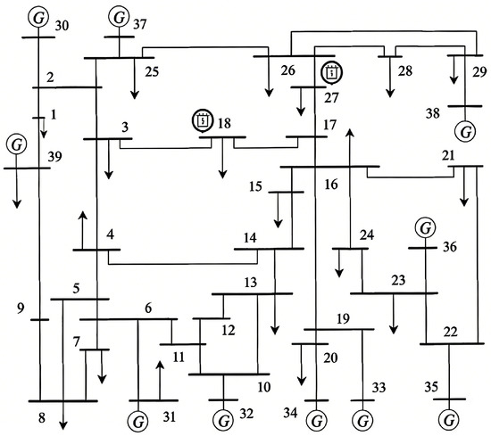
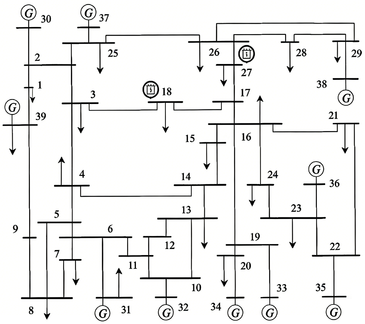
Recalling the DERs problem described in Section 2.3.1, the IEEE 39-bus system, as referenced in [50], is depicted in Figure 1. The system comprises 10 distributed generators (DGs) denoted by the set $D=\left\{30,\dots ,39\right\}$, along with two energy storages (ESs) identified by the set $E=\left\{18,27\right\}$. The system’s primary goal is to achieve economical, effective, and efficient operations through an adeptly engineered coordination and control mechanism for DGs and ESs.

Figure 1. IEEE 39-bus system.

The cost functions for each distributed generator (DG) and energy storage (ES) within the IEEE 39-bus system are characterized by $C_i\left(p_{i,t}\right)=a_i{p}_{i,t}^2+b_i{p}_{i,t}+c_i,t\in T,i\in D$, and $C_i\left(p_{i,t}\right)=d_i\left|p_{i,t}\right|,t\in T,i\in E$, respectively [41]. Here, $p_{i,t}$ represents the power of generator or storage i at time $t\in T$, where $T=\{1,\dots ,t_{end}\}$ denotes the coordination period. The coefficients $a_i,b_i$ and $c_i$ are the cost parameters associated with each DG, while $d_i$ is the cost parameter for each ES. It is noteworthy that the energy storage’s state $E{n}_{i,t_{end}}$ at the end of the period must equal its initial state $E{n}_{i,0}$.

The system also incorporates several constraints. The set $P_i^{DE}$ defines the operational limits for all $i\in D\cup E$ as $P_i^{DE}=\left\{p_i|p_i^{min}\le p_{i,t}\le p_i^{max}\right\}$. For DGs only, $P_i^D$ accounts for ramping constraints $P_i^D=\left\{p_i\right|p_i^{down}$$\le p_{i,t}-p_{i,t-1}\le p_i^{up}\}$ for all $i\in D$, with $p_i^{up}$ and $p_i^{down}$ representing the ramping up and ramping down rates, respectively. For ESs, $P_i^E=\{p_i=p_i^{+}-p_i^{-}|E{n}_{i,min}$$\le E{n}_{i,t}\le E{n}_{i,max},t\in T\}$ for all $i\in E$, where $p_i^{+}$ and $p_i^{-}$ are the charging and discharging powers. The rate of change for ES is denoted by $p_{i,t}^{batt}$, with charging and discharging efficiencies given by ${\kappa }_i^{+},{\kappa }_i^{-}$, respectively. The relationship is defined as:

$$p_{i,t}^{batt}={\displaystyle \frac{p_{i,t}^{+}}{{\kappa }_i^{+}}}-p_{i,t}^{-}{\kappa }_i^{-},E{n}_{i,t}=E{n}_{i,t-1}-p_{i,t}^{batt}\Delta T$$

The power output vector for each i is given by $p_i=\left[p_{i,1},\dots p_{i,t_{end}}\right]$ subject to $p_i\in P_i^{DE}\cup P_i^D\cup P_i^E$. Additionally, the power $p_{i,t}$ at time t is constrained by a coupling constraint ${\sum }_{i=1}^{\left|D\right|+\left|E\right|}{p}_{i,t}=Y_t,t\in T$, where $Y_t$ is the given demand.

Treat the cost function of each DG or ES as $f_i$, the constraints about $p_i$ as $h_i$ and the coupling constraint as $\widehat{g}$ in (2). Subsequently, Algorithm 1 and 2 are leveraged to effectively address the problem.

The parameters for the DGs are detailed in Table 2, while those for the ESs are presented in Table 3. In accordance with Assumption 3, we have configured the maximum step-size parameters as ${\tau }_i=0.9$, ${\sigma }_i=0.005$ and ${\omega }_i=0.05$. Notably, the algorithm guarantees convergence as long as the step-size parameters are strictly bounded by Assumption 3. Empirically, specific choices of these parameters within the valid theoretical regions mainly affect the convergence speed, leaving the overall stability of the system largely stable. Furthermore, the relaxation factor is typically assigned a value of 1.5. With these settings, we proceed to present our results as delineated below.

Table 2. Parameters of DGs.

	Parameters List
${\mathit{DG}}_{\mathit{s}}$	${\mathit{a}}_{\mathit{i}}$ ($/kW2h)	${\mathit{b}}_{\mathit{i}}$ ($/kWh)	${\mathit{c}}_{\mathit{i}}$ ($/h)	${\mathit{p}}_{\mathit{i}}^{\mathit{down}}\mathbf{/}{\mathit{p}}_{\mathit{i}}^{\mathit{up}}$	$[{\mathit{p}}_{\mathit{i}}^{\mathbf{min}},{\mathit{p}}_{\mathit{i}}^{\mathbf{max}}\mathbf{]}$
$D{G}_{30}$	$2.7\times {10}^{-4}$	$1.7\times {10}^{-2}$	$6.6\times {10}^{-1}$	15	[20,180]
$D{G}_{31}$	$3.0\times {10}^{-4}$	$1.4\times {10}^{-2}$	$6.2\times {10}^{-1}$	30	[55,190]
$D{G}_{32}$	$2.5\times {10}^{-4}$	$1.0\times {10}^{-2}$	$1.1\times {10}^{-1}$	55	[20,170]
$D{G}_{33}$	$4.2\times {10}^{-4}$	$1.0\times {10}^{-2}$	$8.3\times {10}^{-1}$	40	[30,170]
$D{G}_{34}$	$2.3\times {10}^{-4}$	$1.7\times {10}^{-2}$	$6.5\times {10}^{-1}$	80	[25,180]
$D{G}_{35}$	$5.3\times {10}^{-4}$	$2.6\times {10}^{-2}$	$3.1\times {10}^{-1}$	50	[40,180]
$D{G}_{36}$	$5.9\times {10}^{-4}$	$1.0\times {10}^{-2}$	$5.7\times {10}^{-1}$	60	[50,190]
$D{G}_{37}$	$4.4\times {10}^{-4}$	$1.5\times {10}^{-2}$	$8.6\times {10}^{-1}$	25	[20,170]
$D{G}_{38}$	$4.0\times {10}^{-4}$	$1.8\times {10}^{-2}$	$0.4\times {10}^{-1}$	65	[35,170]
$D{G}_{39}$	$3.9\times {10}^{-4}$	$2.6\times {10}^{-2}$	$1.6\times {10}^{-1}$	60	[40,180]

Table 3. Parameters of ESs.

	Parameters List
$\mathit{ESs}$	${\mathit{d}}_{\mathit{i}}$ ($/kWh)	$\mathbf{[}{\mathit{E}}_{\mathit{i},\mathbf{0}},{\mathit{E}}_{\mathit{i}}^{\mathbf{max}}\mathbf{]}$	$\mathbf{[}{\mathit{S}}_{\mathit{i}}^{\mathbf{min}},{\mathit{S}}_{\mathit{i}}^{\mathbf{max}}\mathbf{]}$	${\mathit{\kappa }}_{\mathit{i}}^{\mathbf{+}}$	${\mathit{\kappa }}_{\mathit{i}}^{\mathbf{-}}$
$E{S}_{18}$	$1.1\times {10}^{-4}$	[150,550]	[−60,110]	0.8	0.8
$E{S}_{27}$	$1.2\times {10}^{-4}$	[150,450]	[−40,60]	0.9	0.9

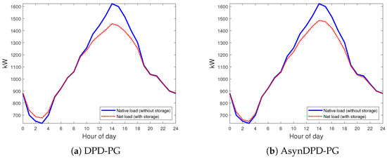
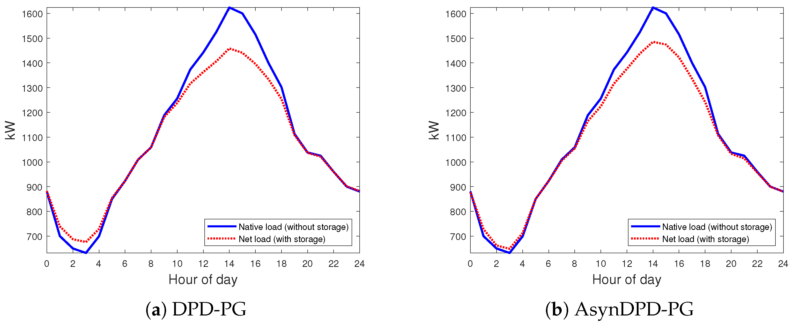
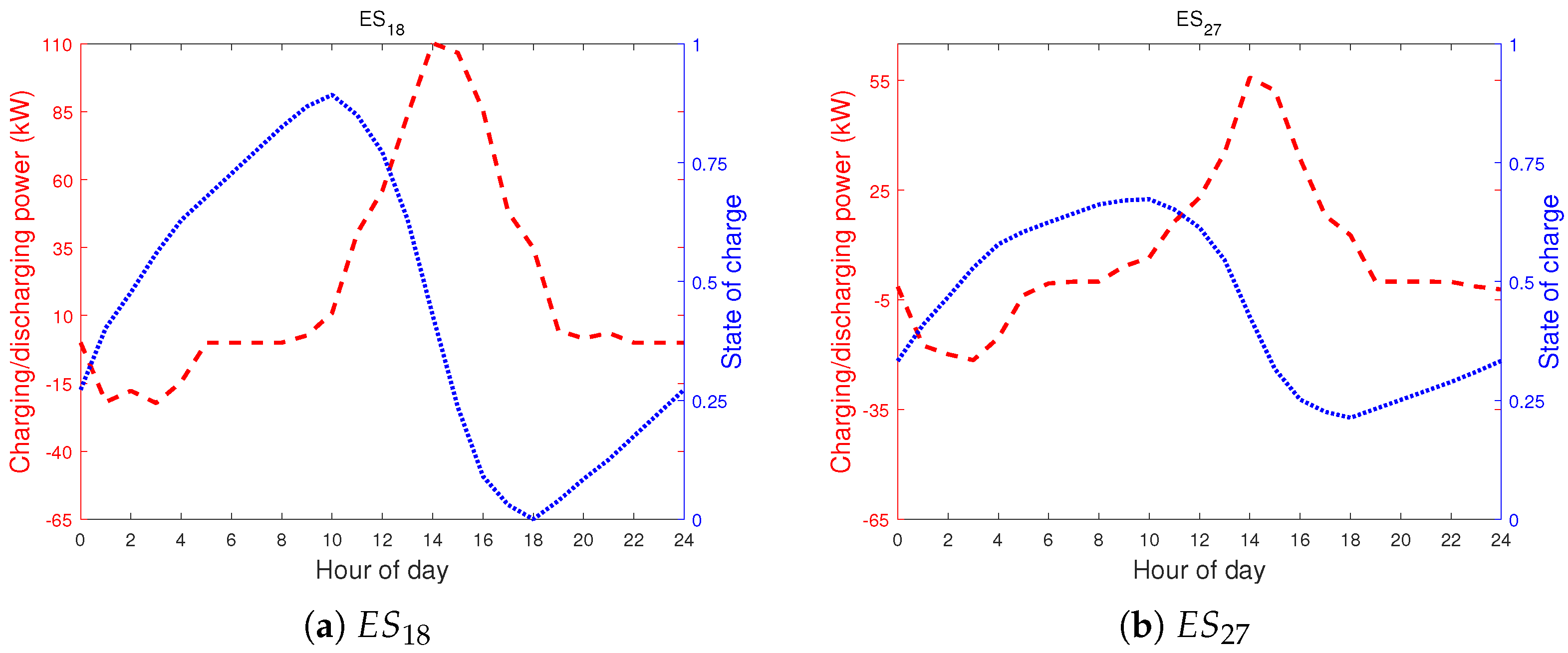
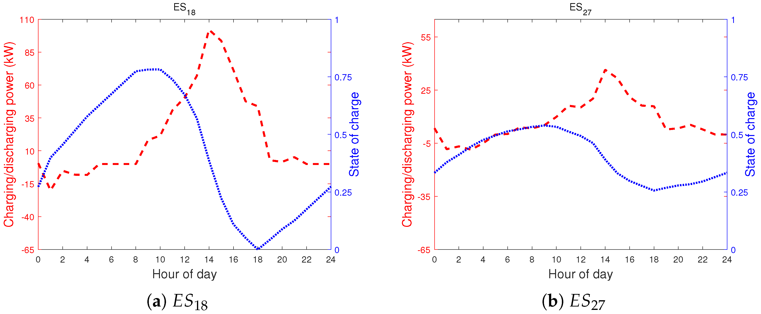
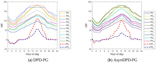
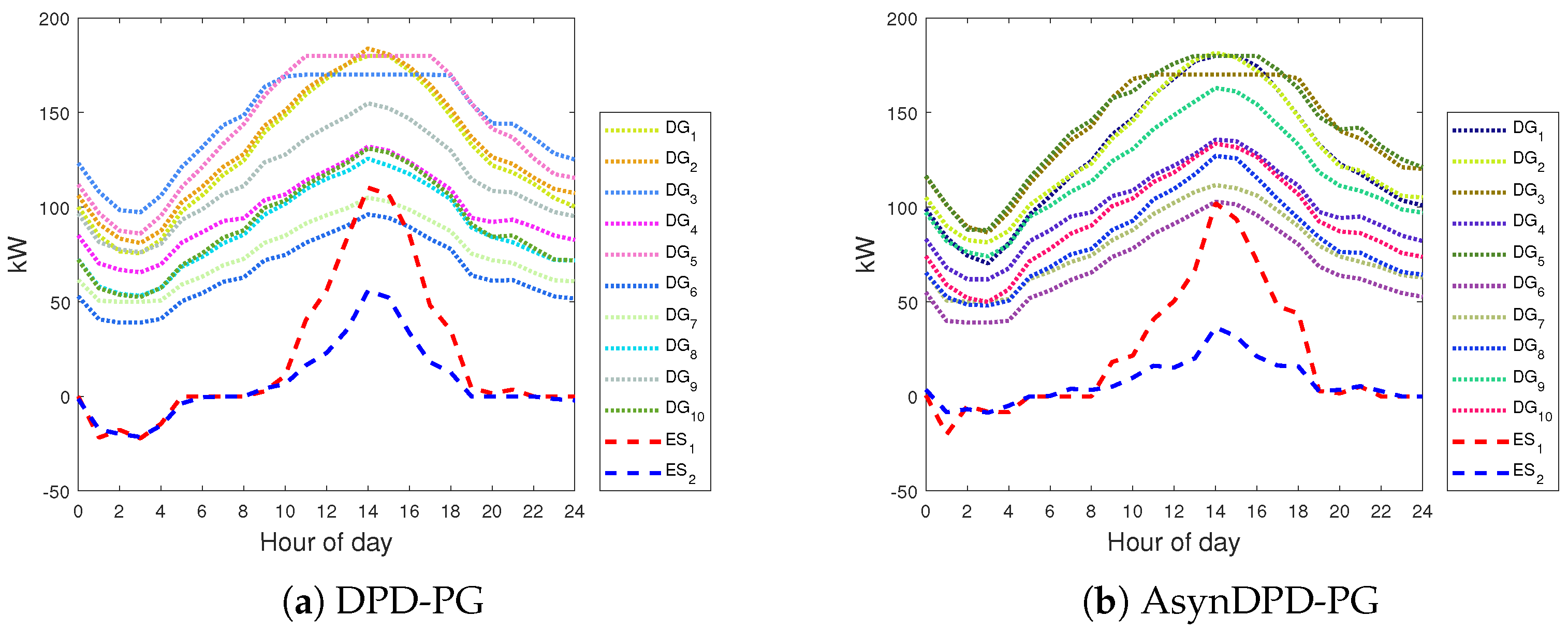
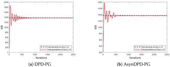
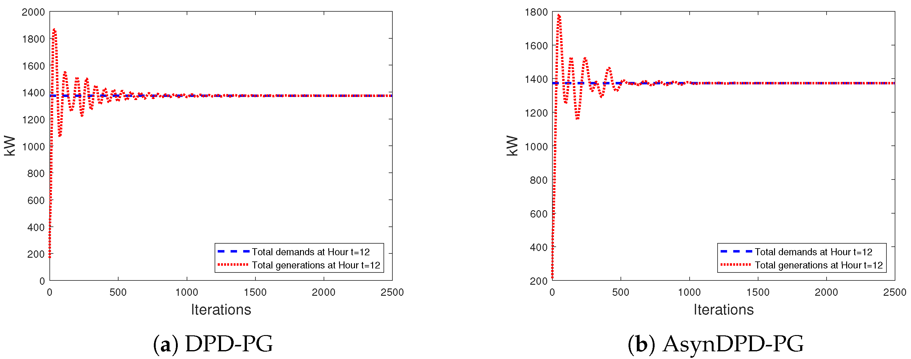
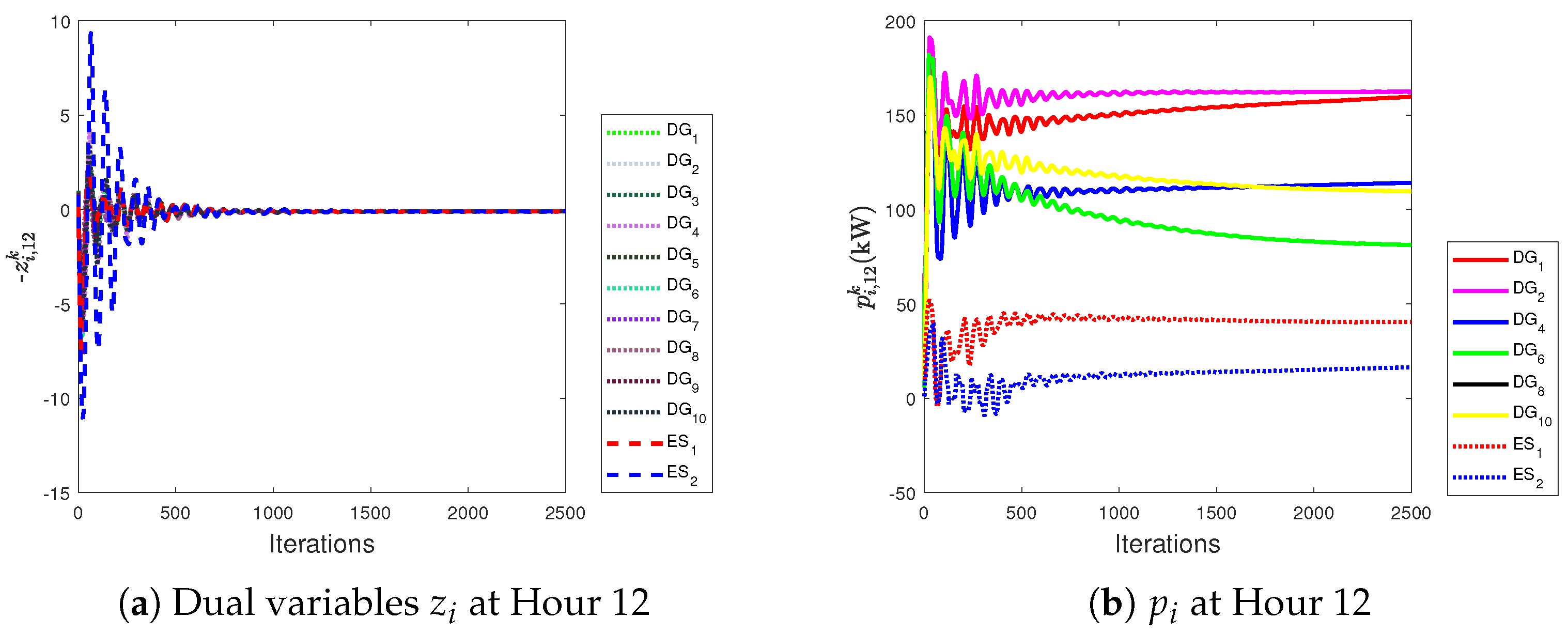
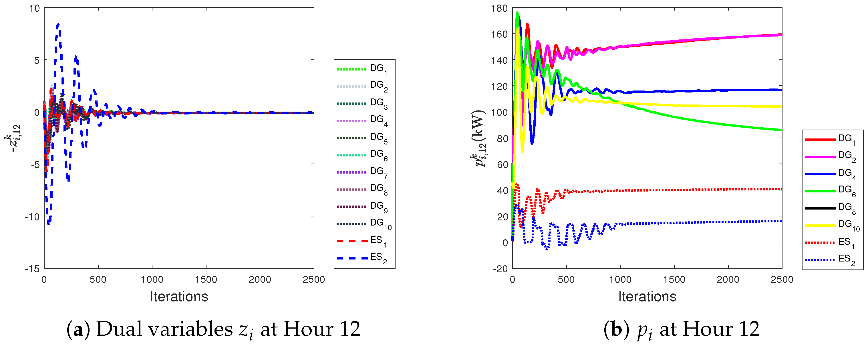
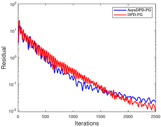
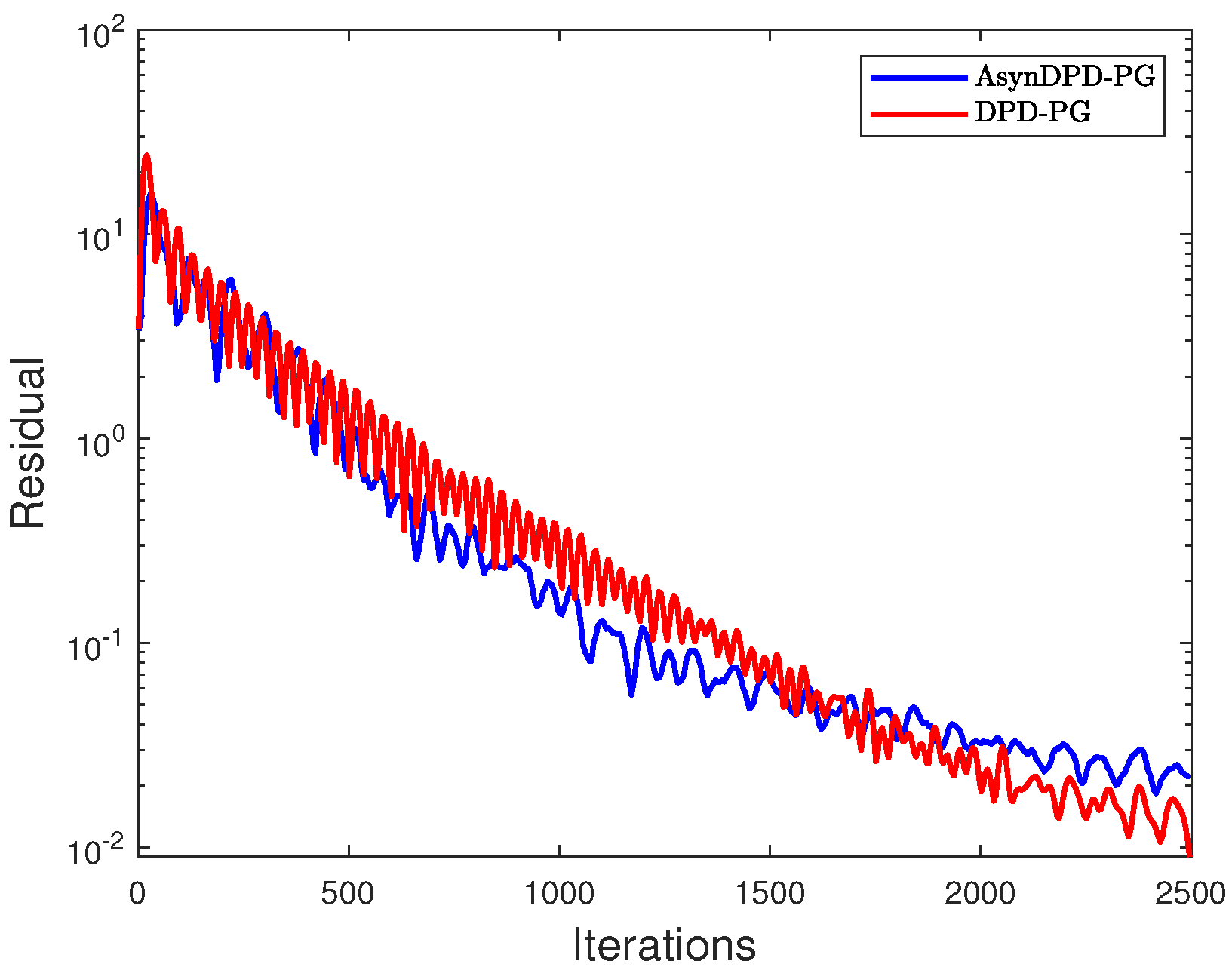
Figure 2 shows the desired effect with storage and without storage for the whole system during the coordination period. It can be seen that ESs fill the valley by charging the system at the off-peak hours (e.g., Hours 2–4), and cut the peak by discharging at peak hours (e.g., Hours 12–16). Figure 3 and Figure 4 show charging and discharging power of ESs and state of charge generated by DPD-PG and AsynDPD-PG, respectively, while the red dotted line indicates charging and discharging power of two ESs, and the blue dotted line indicates state of charge. The transient generations (maybe discharge for ESs) of DGs and ESs during the coordination period are depicted in Figure 5 and it shows the optimal power generations over a day. Figure 6 shows the total demands and total generations of all DGs and ESs at Hour 12. It can be seen that generations fit demands after almost 1500 iterations of DPD-PG and 1200 iterations of AsynDPD-PG. The performance of our algorithms is shown in Figure 7 and Figure 8, in which (a) and (b) show the convergence of dual variables $z_i$ and behaviors of partial $p_i$ at Hour 12, respectively. The residual is defined as $\left(1/\phantom{1m}m\right){\sum }_{i=1}^m∥z_{i,k}-z^{*}∥$. Figure 9 shows the evolution of residuals with the number of iterations for dual variables $z_i$.

Figure 2. Cut the peak and fill the valley.

Figure 3. Charging and discharging power of ESs and state of charge(DPD-PG).

Figure 4. Charging and discharging power of ESs and state of charge(AsynDPD-PG).

Figure 5. Transient generations and optimal power generations.

Figure 6. Total demands and total generations.

Figure 7. Convergence of DPD-PG.

Figure 8. Convergence of AsynDPD-PG.

Figure 9. Evolution of residuals.

Furthermore, while Figure 2, Figure 3, Figure 4, Figure 5, Figure 6, Figure 7, Figure 8 and Figure 9 visually demonstrate the convergence and the practical application effects of the proposed algorithms, qualitative plots alone are insufficient to fully illustrate their computational efficiency. To make a stronger quantitative case, Table 4 summarizes the explicit performance metrics of DPD-PG and AsynDPD-PG from the simulation results.

Table 4. Quantitative performance of the proposed algorithms.

Algorithm	Iterations (to Reach Steady State)	Residual (at 2500 Iterations)
DPD-PG	∼1500	∼1.0 × ${10}^{-2}$
AsynDPD-PG	∼1200	∼2.0 × ${10}^{-2}$

As quantitatively shown in Table 4, both proposed algorithms achieve desired precision with final residuals dropping to the order of ${10}^{-2}$. Notably, the asynchronous algorithm, AsynDPD-PG, demonstrates a distinct advantage in convergence speed. It reaches a steady state in approximately 1200 iterations, outperforming the synchronous DPD-PG, which requires around 1500 iterations. This quantitative evidence explicitly confirms that the asynchronous implementation effectively accelerates the convergence process by reducing the required iteration counts, thereby making it highly suitable for large-scale multi-agent systems where communication delays often occur.

5.2. Logistic Regression Problem

Following the logistic regression problem described in Section 2.3.2, the breast cancer data set from the UCI Machine Learning Repository [51] is leveraged here to generate a concrete numerical experiment. Notably, we treat this purely as an optimization problem to verify the convergence and efficiency of our algorithms, rather than evaluating a machine learning model’s predictive ability. Therefore, we bypass the standard machine learning pipeline (i.e., without model training and testing). Specifically, we extract a subset of 400 samples from the dataset solely to construct the objective function of the distributed logistic regression problem on an m-agent network. Each agent holds $q_i$ h-th training samples $(c_{i,h},l_{i,h})$ with data vector $c_{i,h}\in {\mathbf{R}}^9$ and label constant $l_{i,h}\in \{-1,1\}$, where ${\sum }_{i=1}^m{\sum }_{h=1}^{q_i}{q}_i=N,i=1,\dots ,m,h=1,\dots ,q_i$. The optimal solution of problem (6) is the maximum log likelihood estimate of the classifier x. Considering the regularization terms, problem (6) is reformulated as

$${\widehat{x}}^{*}=arg\underset{x\in {\mathbf{R}}^n}{min}{\displaystyle \frac{\mu }{2}}{∥\widehat{x}∥}^2+{\displaystyle \sum _{i=1}^m}{\displaystyle \sum _{h=1}^{q_i}}ln\left(1+exp\left(-l_{i,h}{c}_{i,h}^{\mathrm{T}}\widehat{x}\right)\right)+\gamma {∥\widehat{x}∥}_1$$

(29)

where L1 regularization term $\gamma {∥x∥}_1$ is leveraged to make the optimal solution sparse and L2 regularization term ${\displaystyle \frac{\mu }{2}}{∥x∥}^2$ is added to avoid overfitting. Notice that $\widehat{x}$ is shared by all agents, the local variable $x_i$ is introduced to estimate $\widehat{x}$. Meanwhile, there is a constraint $(\mathcal{L}\otimes I)x=0$, where $x=\mathrm{col}{\left\{x_i\right\}}_{i=1}^m$ and $\mathcal{L}$ is Laplacian matrix of network. Let $A_i={\mathcal{L}}_i\otimes I$, where ${\mathcal{L}}_i$ is the i-th column of the Laplacian matrix $\mathcal{L}$. Then problem (29) can be transformed into problem (2) through setting as follows

$$\begin{array}{c}{f}_i\left(x_i\right)={\displaystyle \frac{\mu }{2m}}{∥x_i∥}^2+{\displaystyle \sum _{h=1}^{q_i}}ln\left(1+exp\left(-l_{i,h}{c}_{i,h}^{\mathrm{T}}{x}_i\right)\right)\hfill \\ h_i\left(x_i\right)={\displaystyle \frac{\gamma }{m}}{∥x_i∥}_1\hfill \\ \widehat{g}\left({\sum }_{i=1}^m{A}_i{x}_i\right)={\delta }_{\left\{0\right\}}\left((\mathcal{L}\otimes I)x\right)\hfill \end{array}$$

Clearly, the specific formulations of these functions satisfy the properties mentioned in Section 2.2 and Assumption 2. Subsequently, Algorithms 1 and 2 are leveraged to solve the problem. The network topology is generated randomly with agents $m=40$. To satisfy Assumption 3, we have configured the maximum step-size parameters as ${\tau }_i=0.01$, ${\sigma }_i=0.001$, and ${\omega }_i=0.6$. Furthermore, the relaxation factor is typically assigned a value of 1.5. In Algorithm 2, the activated probability of each agent $p_i$ is set between 0.1 and 0.9.

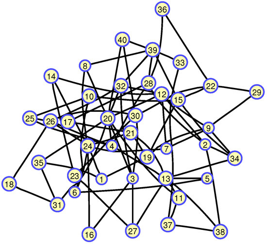
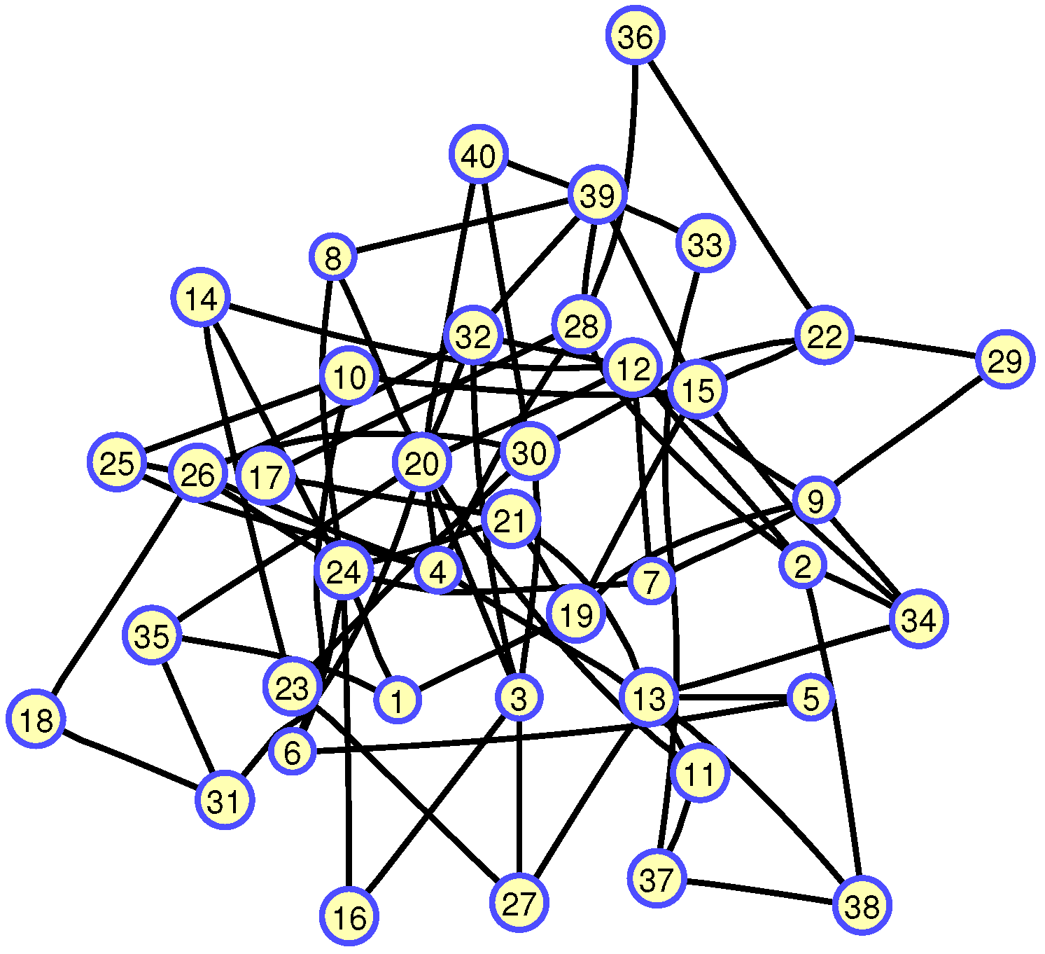
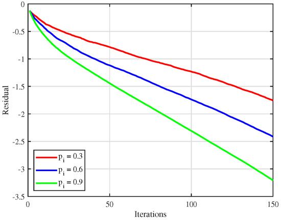
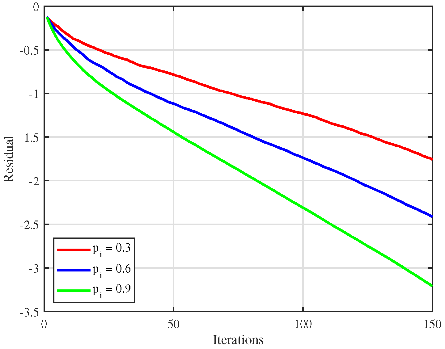
The communication network is shown in Figure 10. To demonstrate the performance of the asynchronous design, a sensitivity test is conducted on the activation probabilities $p_i$ for AsynDPD-PG. We test the algorithm under different activation probability settings, specifically $p_i\in \left\{0.3,0.6,0.9\right\}$, while keeping other parameters constant. The evolution of the residuals under these different settings is depicted in Figure 11.

Figure 10. Network topology.

Figure 11. Sensitivity analysis of AsynDPD-PG with different activation probabilities.

Notably, while Theorem 2 guarantees theoretical convergence as long as $p_i>0$ for all agents, the practical convergence speed will be significantly affected by the activation probability $p_i$. In the considered network, agents with extremely small activation probabilities act as stragglers. Since the distributed algorithm ultimately requires all agents to reach the global optimal solution, the fast-updating nodes will eventually be bottlenecked by the delayed information from these stragglers. Consequently, the overall empirical convergence rate of the system is largely dominated by the minimum activation probability in the network. From a practical engineering perspective, this implies that reasonably allocating computing and communication resources to avoid the presence of extremely slow nodes with $p_i\to 0$ is crucial for enhancing the overall operational efficiency of the asynchronous algorithm.

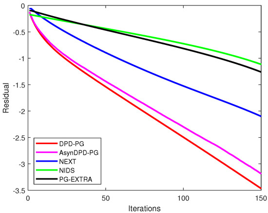
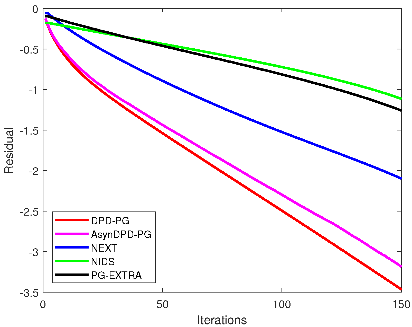
To evaluate the performance of our algorithms, we compare our algorithms with PG-EXTRA [24], NEXT [28] and NIDS [52]. It is worth noting that while these methods are not able to handle the problem (2), they are fully applicable to the logistic regression problem here. Therefore, this common application is utilized to establish the performance comparison. For each algorithm, the parameters are empirically selected within their theoretically guaranteed convergence ranges to ensure a stable and convergent behavior. Define the residual as $\left(1/\phantom{1m}m\right){log}_{10}$$\left({\sum }_{i=1}^m∥x_{i,k}-x_i^{*}∥\right)$. Figure 12 illustrates the evolution of the residual relative to the number of iterations. To further clarify the comparison, Table 5 summarizes the quantitative performance.

Figure 12. Performance comparison.

Table 5. Quantitative comparison of convergence performance.

Metrics	DPD-PG	AsynDPD-PG	NEXT	NIDS	PG-EXTRA
Residual at 150 iterations (${log}_{10}$)	∼−3.5	∼−3.2	∼−2.1	∼−1.1	∼−1.2
Iterations to reach ${10}^{-2}$ residual	∼82	∼90	∼142	>150	>150

It can be observed that DPD-PG almost reaches a residual level of ${10}^{-3.5}$ at the 150th iteration, while NIDS and PG-EXTRA only reach a level of nearly ${10}^{-1.1}$ and ${10}^{-1.2}$, respectively. Furthermore, to achieve an accuracy on the order of ${10}^{-2}$, DPD-PG and AsynDPD-PG require approximately 82 and 90 iterations, while NEXT requires nearly 142 iterations.

6. Conclusions

This paper focuses on a convex optimization problem characterized by a composite objective function that comprises a local convex smooth function, a nonsmooth one and a nonseparable coupling function possibly nonsmooth. DPD-PG and its asynchronous version AsynDPD-PG are proposed to tackle this problem. The algorithms are crafted using primal-dual theory and proximal gradient techniques, leveraging KKT conditions for its design. Drawing on the operator splitting theory, we establish the convergence of two algorithms under necessary assumptions. By solving a dynamic resource coordination problem, the effectiveness of the algorithm and the correctness of the theoretical analysis are demonstrated. Looking ahead, our future research will introduce stochastic gradients into the algorithm, aiming to enhance adaptability and efficiency in time-varying and directed networks.

References

- Saeed Osman, M. Last-mile decomposition heuristics with multi-period embedded optimization models. Math. Comput. Appl. 2025, 30, 90. [Google Scholar] [CrossRef] [Scilit]
- Ding, Y.; Ren, W.; Meng, Z. Distributed optimal time-varying resource allocation for networked high-order systems. IEEE Trans. Autom. Control 2024, 69, 5899–5914. [Google Scholar] [CrossRef] [Scilit]
- Wu, H.; Liu, Q.; Park, J.H. Adaptive fuzzy-based distributed optimization with privacy protection for uncertain high-order nonlinear multi-agent systems against two types of cyber attacks. J. Frankl. Inst. 2025, 362, 107769. [Google Scholar] [CrossRef] [Scilit]
- Li, H.; Fan, L.; Ran, L.; Wang, Z.; Zheng, Z.; Li, Z.; Li, S.; Zheng, L.; Li, J. Edge-based distributed primal-dual algorithms for seeking generalized Nash equilibria. Eur. J. Control 2024, 77, 100990. [Google Scholar] [CrossRef] [Scilit]
- Wan, Y.; Qin, J.; Li, F.; Yu, X.; Kang, Y. Game theoretic-based distributed charging strategy for PEVs in a smart charging station. IEEE Trans. Smart Grid 2020, 12, 538–547. [Google Scholar] [CrossRef] [Scilit]
- Doostmohammadian, M.; Ghods, A.A.; Aghasi, A.; Gabidullina, Z.R.; Rabiee, H.R. Using non-Lipschitz signum-based functions for distributed optimization and machine learning: Trade-off between convergence rate and optimality gap. Math. Comput. Appl. 2025, 30, 108. [Google Scholar] [CrossRef] [Scilit]
- Gang, A.; Xiang, B.; Bajwa, W.U. Distributed principal subspace analysis for partitioned big data: Algorithms, analysis, and implementation. IEEE Trans. Signal Inf. Process. Netw. 2021, 7, 699–715. [Google Scholar] [CrossRef] [Scilit]
- Condat, L. A primal-dual splitting method for convex optimization involving Lipschitzian, proximable and linear composite terms. J. Optim. Theory Appl. 2013, 158, 460–479. [Google Scholar] [CrossRef] [Scilit]
- Tang, Y.; Wu, G. A general framework for solving convex optimization problems involving the sum of three convex functions. Sci. Sin. Math. 2019, 49, 1073–1106. [Google Scholar]
- Combettes, P.L.; Pesquet, J.C. Primal-dual splitting algorithm for solving inclusions with mixtures of composite, Lipschitzian, and parallel-sum type monotone operators. Set-Valued Var. Anal. 2012, 20, 307–330. [Google Scholar] [CrossRef] [Scilit]
- Komodakis, N.; Pesquet, J.C. Playing with duality: An overview of recent primal-dual approaches for solving large-scale optimization problems. IEEE Signal Process. Mag. 2015, 32, 31–54. [Google Scholar] [CrossRef] [Scilit]
- Huang, W.; Li, H.; Peng, J.; Tang, Y.; He, H. Simplified primal-dual forward-backward splitting algorithm for solving structured monotone inclusion with applications. J. Nonlinear Var. Anal. 2025, 9, 927–945. [Google Scholar]
- Yin, C.; Xu, H.W.; Yang, J.F. A modified primal-dual algorithm for structured convex optimization with a Lipschitzian term. J. Oper. Res. Soc. China 2024. [Google Scholar] [CrossRef] [Scilit]
- Nedic, A.; Olshevsky, A. Distributed optimization over time-varying directed graphs. IEEE Trans. Autom. Control 2015, 60, 601–615. [Google Scholar] [CrossRef] [Scilit]
- Xi, C.; Khan, U.A. Directed-distributed gradient descent. In Proceedings of the 2015 53rd Annual Allerton Conference on Communication, Control, and Computing (Allerton), Monticello, IL, USA, 29 September–2 October 2015; pp. 1022–1026. [Google Scholar]
- Shi, W.; Ling, Q.; Wu, G.; Yin, W. EXTRA: An exact first-order algorithm for decentralized consensus optimization. SIAM J. Optim. 2015, 25, 944–966. [Google Scholar] [CrossRef] [Scilit]
- Xi, C.; Khan, U.A. DEXTRA: A fast algorithm for optimization over directed graphs. IEEE Trans. Autom. Control 2017, 62, 4980–4993. [Google Scholar] [CrossRef] [Scilit]
- Maros, M.; Jalden, J. On the Q-linear convergence of distributed generalized ADMM under non-strongly convex function components. IEEE Trans. Signal Inf. Process. Netw. 2019, 5, 442–453. [Google Scholar] [CrossRef] [Scilit]
- Carnevale, G.; Bastianello, N.; Notarstefano, G.; Carli, R. ADMM-tracking gradient for distributed optimization over asynchronous and unreliable networks. IEEE Trans. Autom. Control 2025, 70, 5160–5175. [Google Scholar] [CrossRef] [Scilit]
- Chen, J.; Liu, S.; Chen, P. Zeroth-order diffusion adaptation over networks. In Proceedings of the 2018 IEEE International Conference on Acoustics, Speech and Signal Processing (ICASSP), Calgary, AB, Canada, 15–20 April 2018; pp. 4324–4328. [Google Scholar]
- Nedic, A.; Olshevsky, A.; Shi, W. Achieving geometric convergence for distributed optimization over time-varying graphs. SIAM J. Optim. 2017, 27, 2597–2633. [Google Scholar] [CrossRef] [Scilit]
- Pu, S.; Shi, W.; Xu, J.; Nedic, A. Push-pull gradient methods for distributed optimization in networks. IEEE Trans. Autom. Control 2021, 66, 1–16. [Google Scholar] [CrossRef] [Scilit]
- Su, Y.; Wang, Q.; Sun, C. Distributed primal-dual method for convex optimization with coupled constraints. IEEE Trans. Signal Process. 2022, 70, 523–535. [Google Scholar] [CrossRef] [Scilit]
- Shi, W.; Ling, Q.; Wu, G.; Yin, W. A proximal gradient algorithm for decentralized composite optimization. IEEE Trans. Signal Process. 2015, 63, 6013–6023. [Google Scholar] [CrossRef] [Scilit]
- Guo, L.; Shi, X.; Cao, J.; Wang, Z. Decentralized inexact proximal gradient method with network-independent stepsizes for convex composite optimization. IEEE Trans. Signal Process. 2023, 71, 786–801. [Google Scholar] [CrossRef] [Scilit]
- Guo, L.; Shi, X.; Yang, S.; Cao, J. DISA: A dual inexact splitting algorithm for distributed convex composite optimization. IEEE Trans. Autom. Control 2024, 69, 2995–3010. [Google Scholar] [CrossRef] [Scilit]
- Aybat, N.S.; Wang, Z.; Lin, T.; Ma, S. Distributed linearized alternating direction method of multipliers for composite convex consensus optimization. IEEE Trans. Autom. Control 2018, 63, 5–20. [Google Scholar] [CrossRef] [Scilit]
- Lorenzo, P.D.; Scutari, G. NEXT: In-network nonconvex optimization. IEEE Trans. Signal Inf. Process. Netw. 2016, 2, 120–136. [Google Scholar] [CrossRef] [Scilit]
- Xu, J.; Tian, Y.; Sun, Y.; Scutari, G. Distributed algorithms for composite optimization: Unified framework and convergence analysis. IEEE Trans. Signal Process. 2021, 69, 3555–3570. [Google Scholar] [CrossRef] [Scilit]
- Scutari, G.; Sun, Y. Distributed nonconvex constrained optimization over time-varying digraphs. Math. Program. 2019, 176, 497–544. [Google Scholar] [CrossRef] [Scilit]
- Yin, C.; Yang, J. Golden ratio proximal gradient ADMM for distributed composite convex optimization. J. Optim. Theory Appl. 2024, 200, 895–922. [Google Scholar] [CrossRef] [Scilit]
- Bianchi, P.; Hachem, W.; Iutzeler, F. A coordinate descent primal-dual algorithm and application to distributed asynchronous optimization. IEEE Trans. Autom. Control 2016, 61, 2947–2957. [Google Scholar] [CrossRef] [Scilit]
- Notarnicola, I.; Notarstefano, G. Asynchronous distributed optimization via randomized dual proximal gradient. IEEE Trans. Autom. Control 2017, 62, 2095–2106. [Google Scholar] [CrossRef] [Scilit]
- Alghunaim, S.A.; Yan, M.; Sayed, A.H. A multi-agent primal-dual strategy for composite optimization over distributed features. In Proceedings of the 2020 28th European Signal Processing Conference (EUSIPCO), Amsterdam, The Netherlands, 18–21 January 2021; pp. 2095–2099. [Google Scholar]
- Shorinwa, O.; Schwager, M. Distributed model predictive control via separable optimization in multiagent networks. IEEE Trans. Autom. Control 2024, 69, 230–245. [Google Scholar] [CrossRef] [Scilit]
- Chambolle, A.; Pock, T. A first-order primal-dual algorithm for convex problems with applications to imaging. J. Math. Imag. Vis. 2011, 40, 120–145. [Google Scholar] [CrossRef] [Scilit]
- O’Donoghue, B.; Stathopoulos, G.; Boyd, S. A splitting method for optimal control. IEEE Trans. Control Syst. Technol. 2013, 21, 2432–2442. [Google Scholar] [CrossRef] [Scilit]
- Latafat, P.; Freris, N.M.; Patrinos, P. A new randomized block-coordinate primal-dual proximal algorithm for distributed optimization. IEEE Trans. Autom. Control 2019, 64, 4050–4065. [Google Scholar] [CrossRef] [Scilit]
- Xu, J.; Zhu, S.; Soh, Y.C.; Xie, L. A dual splitting approach for distributed resource allocation with regularization. IEEE Trans. Control Netw. Syst. 2019, 6, 403–414. [Google Scholar] [CrossRef]
- Alghunaim, S.A.; Lyu, Q.; Yuan, K.; Sayed, A.H. Dual consensus proximal algorithm for multi-agent sharing problems. IEEE Trans. Signal Process. 2021, 69, 5568–5579. [Google Scholar] [CrossRef] [Scilit]
- Yang, T.; Wu, D.; Fang, H.; Ren, W.; Wang, H.; Hong, Y. Distributed energy resource coordination over time-varying directed communication networks. IEEE Trans. Control Netw. Syst. 2019, 6, 1124–1134. [Google Scholar] [CrossRef] [Scilit]
- Yi, P.; Pavel, L. Asynchronous distributed algorithms for seeking generalized Nash equilibria under full and partial-decision information. IEEE Trans. Cybern. 2019, 50, 2514–2526. [Google Scholar] [CrossRef] [Scilit]
- Wu, D.; Yang, T.; Stoorvogel, A.A.; Stoustrup, J. Distributed optimal coordination for distributed energy resources in power systems. IEEE Trans. Autom. Sci. Eng. 2017, 14, 414–424. [Google Scholar] [CrossRef] [Scilit]
- Yang, T.; Yi, X.; Wu, J.; Yuan, Y.; Wu, D.; Meng, Z.; Hong, Y.; Wang, H.; Lin, Z.; Johansson, K.H. A survey of distributed optimization. Annu. Rev. Control 2019, 47, 278–305. [Google Scholar] [CrossRef] [Scilit]
- Bauschke, H.H.; Combettes, P.L. Convex Analysis and Monotone Operator Theory in Hilbert Spaces, 1st ed.; Springer: Cham, Switzerland, 2011. [Google Scholar]
- Ren, W.; Beard, R.W. Consensus seeking in multiagent systems under dynamically changing interaction topologies. IEEE Trans. Autom. Control 2005, 50, 655–661. [Google Scholar] [CrossRef] [Scilit]
- Cortés, J. Distributed algorithms for reaching consensus on general functions. Automatica 2008, 44, 726–737. [Google Scholar] [CrossRef] [Scilit]
- Mansoori, F.; Wei, E. A fast distributed asynchronous Newton-based optimization algorithm. IEEE Trans. Autom. Control 2020, 65, 2769–2784. [Google Scholar] [CrossRef] [Scilit]
- Hong, M.; Chang, T.-H. Stochastic proximal gradient consensus over random networks. IEEE Trans. Signal Process. 2017, 65, 2933–2948. [Google Scholar] [CrossRef] [Scilit]
- IEEE 39-Bus System. Available online: https://icseg.iti.illinois.edu/ieee-39-bus-system/ (accessed on 12 March 2026).
- Dua, D.; Graff, C. UCI Machine Learning Repository. Available online: http://archive.ics.uci.edu/ml (accessed on 12 March 2026).
- Li, Z.; Shi, W.; Yan, M. A decentralized proximal-gradient method with network independent step-sizes and separated convergence rates. IEEE Trans. Signal Process. 2019, 67, 4494–4506. [Google Scholar] [CrossRef] [Scilit]
Disclaimer/Publisher’s Note: The statements, opinions and data contained in all publications are solely those of the individual author(s) and contributor(s) and not of MDPI and/or the editor(s). MDPI and/or the editor(s) disclaim responsibility for any injury to people or property resulting from any ideas, methods, instructions or products referred to in the content. |
© 2026 by the authors. Licensee MDPI, Basel, Switzerland. This article is an open access article distributed under the terms and conditions of the Creative Commons Attribution (CC BY) license.