Development and Optimization of Cattaneo–Christov Carreau–Yasuda Tri-Hybrid Nanofluid Using Artificial Neural Networks

Abstract

An artificial neural network (ANN) prediction model based on the Levenberg–Marquardt (LM) algorithm has been developed to predict the nonlinear heat and mass transfer characteristics of Cattaneo–Christov Carreau–Yasuda tri-hybrid nanofluid (CCHMF–THNF) flow over a porous stretching sheet. A mathematical model of the phenomenon was developed based on a number of elements, including the combined effect of magnetohydrodynamic forces, thermal and solutal relaxation and the influence of viscoelastic fluid behavior and is numerically analyzed utilizing MATLAB bvp4c software. A set of standard data was generated as a reference for developing the ANN-LM model with one hidden layer containing 10 neurons and log-sigmoid activation function, to achieve rapid predictions of velocity, temperature and concentration profiles from the identified data set. This study introduces a novel methodology to provide fast prediction capabilities for transport characteristics through integration of the ANN–LM model with the non-linear CCHMF-THNF model, producing computational savings by providing prediction accuracy of transport characteristics with MSE values on the order of $1.0\times {10}^{-10}$ using ANN–LM in place of repeated bvp4c solutions. Furthermore, the predictive capability of the developed ANN–LM framework may be beneficial in the areas of thermal management systems, polymer processing, energy transport applications, and magnetically controlled cooling technologies since they all share a need for fast access to transportation characteristic evaluation data.

1. Introduction

Because of its excellent ability to handle difficult nonlinear curve-fitting issues, LM is a technique that is crucial for modelling Carreau–Yasuda tri-nanofluids. Shear-thinning behavior and viscoelastic qualities are demonstrated by the dynamic changing of fluid viscosity in shear rates in non-Newtonian fluids, such as Carreau–Yasuda fluids. When three distinct kinds of nanoparticles are dispersed in the base fluid, the interactions between the nanoparticles become more complicated and contribute to the viscosity behavior of the tri-nanofluid. Since the process requires accurate parameter estimates to reflect the rheological features, modelling it is extremely difficult. The aforementioned problem was solved using the LM methodology, which combined the Gauss–Newton and gradient descent methods to make it converge on the ideal values. The LM technique is therefore made resilient for both non-convex and nonlinear models by this hybrid approach, which also allows the parameters to be refined even when they are situated far from the ultimate solution. Carreau–Yasuda models of tri-nanofluids are much improved by LM, according to the reduction of differences between predicted and experimental findings. Thus, these models may be used to simplify the job of designers in fields where regulated action regarding fluid behaviour is crucial, including biomedical, energy systems, or pure materials research.

Heat and mass transport in non-Newtonian fluids is receiving increased interest due to its relevance to applications in the biomedical engineering field, energy systems, and various industrial processes. The family of rheological models features the Carreau–Yasuda fluid that can account for shear-thinning behavior and shear-thickening behavior that can be used to model complex fluids such as blood, polymer solutions, and nanofluids [1]. Nanofluids, which are a base fluid that has been enhanced by the inclusion of nanoparticles, have radically improved thermal systems for rates of heat transfer of many types of materials. Research has evolved from mono-nanofluids to hybrid nanofluids and tri-nanofluids with encouraging rates of improvement of the Thermophysical properties of materials [2]. Tri-nanofluids, which can utilize three distinct types of nanoparticles such as $A{l}_2{O}_3, F{e}_3{O}_4$ or $Ti{O}_2$, will exhibit superior thermal conductivity and mass diffusivity, particularly in terms of how the behavior of the fluid interacts with magnetohydrodynamics (MHD) and convective conditions. Carreau–Yasuda tri-nanofluids have been analyzed in several parameterized quasi-two-dimensional setups, including stretching surfaces, porous media and stagnation point flows. The gyrotactic bio convection in Carreau–Yasuda nanofluids was studied by Alahmadi and Alkinidri [3] and their study concluded results of improved thermal effectiveness due to interaction of particles supporting bio convection. Rauf et al. [4] investigated the mixed convection in tri-hybrid nanofluids, with the validation of results showing favorable Nusselt and Sherwood numbers as a result of thermophoresis and Brownian motion. Solving the governing nonlinear partial differential equations (PDEs) through traditional numerical methods (e.g., finite difference and shooting techniques) can be a cumbersome process, experiencing significant limitations when considering greater dimensional parameter spaces [5].

AI-supported optimization techniques, backed by neural network methods, have shown promise in predicting profiles of velocity, temperature, and concentration with very accurate results. Some hybrid computational frameworks would depend on back-propagated neural networks and genetic algorithms, along with the foundation of sequential quadratic programming (SQP) optimization methods to increase heat and mass transfer in non-Newtonian fluids. Khan et al. [6] implemented deep learning models to predict the entropy generation in magnetohydrodynamic Carreau–Yasuda flows and validated their models by obtaining good agreement with their experimental data. Recent developments in computational modeling have greatly improved the investigation of heat and mass transfer in nanofluids. Specifically, Gupta et al. [7] constructed an artificial neural network (ANN) model trained via the Levenberg–Marquardt learning algorithm to estimate heat transfer characteristics in flow between two rotating disks with an Ag-TiO₂/water hybrid nanofluid. The study indicated high accuracy in predicting Nusselt numbers, with regression values greater than 0.99, demonstrating the ANN’s ability to make accurate thermal predictions. In another contribution, Gupta [8] used the differential transform method (DTM) to investigate magnetohydrodynamic (MHD) flow of a rotating micropolar fluid between two parallel plates. The results demonstrated the influence of magnetic field strength, porosity, and rotation parameters, in terms of velocity profiles and skin friction, which further validated the DTM’s semi-analytical approach. To advance the use of DTM, Gupta et al. [9] investigated the squeezing flow of an iron oxide polymer nanofluid being formed between electromagnetic Riga plates with the effects of heat source/sink and chemical reaction. The results emphasized the electromagnetic forces for increased control of the fluid solutions and the major parameters impacting temperature and concentration distributions. Recent research has focused extensively on the effects of multi-component nanofluids and non-Newtonian base fluids on convective heat transfer under the effects of magnetohydrodynamics (MHD), radiation and porous media. For example, several studies of hybrid Cu–Al₂O₃/water flows over stretching geometries demonstrated substantial thermal enhancements when the flow also had an inclined magnetic field, viscous dissipation, plus internal sources/sinks of heat [10]. Quadra- and ternary-hybrid systems have also been studied for more complex base fluids—including the addition of various nanoparticle species that can improve thermal diffusion and change critical shear-rate behavior, such as engine-oil-based quadra-hybrid models [11], or dissipative Casson ternary hybrid flows with nonuniform thermal–mass distributions across flat plates [12]. Many other studies have translated this vision into other physics, demonstrating effects on stability and thermal fields due to bio-convection and radiation [13]. Experiments on MHD stagnation-point and stretching-sheet flows for mixed non-Newtonian models demonstrate how viscous dissipation, suction/injection, and porous Darcy–Forchheimer resistance make substantial modifications to boundary-layer structure and surface transfer rates [14,15]. Finally, entropy generation optimization and Arrhenius-activation-energy treatment for Carreau–Yasuda nanofluids serve to demonstrate how thermodynamic irreversibility and chemical reaction kinetics further impact performance measures in MHD stagnation flows [16]. Research has more recently stressed how important it is to enhance the stability and create sustainable formulations of nanofluids. This is especially true concerning the role surfactants play in determining the thermophysical characteristics of the fluid and the durability of the fluid for use in long-term-potential engineering applications [17].

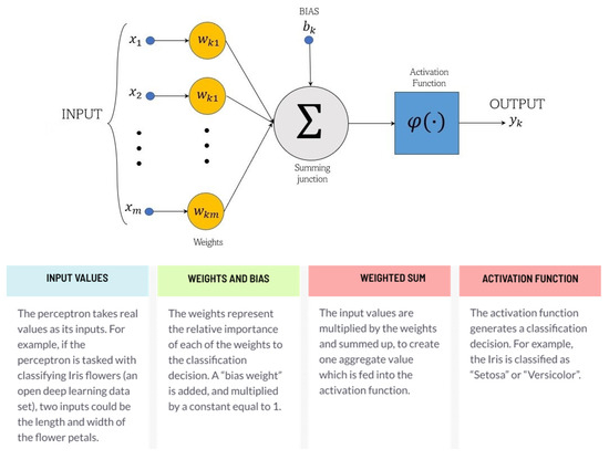
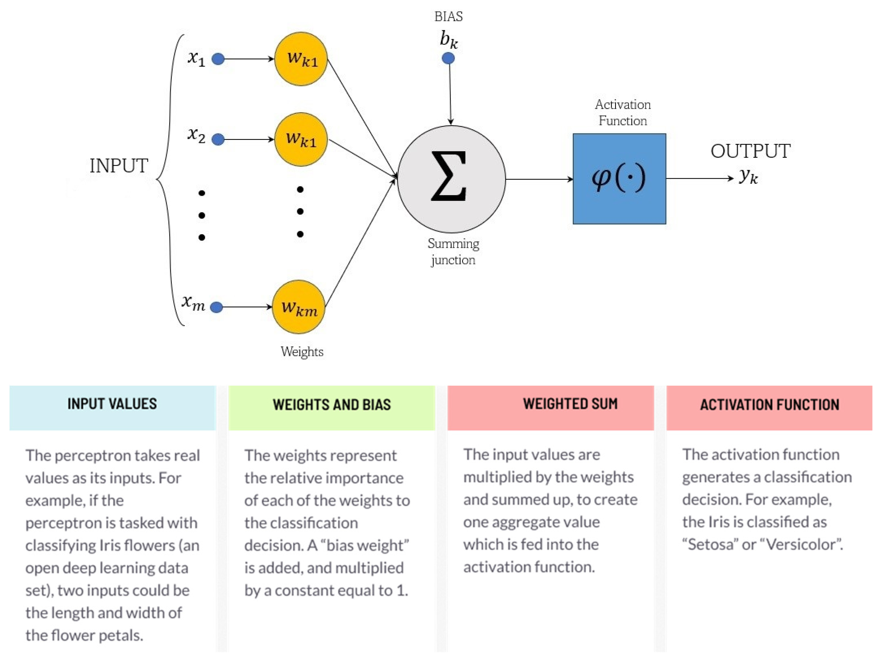
An artificial neural network (ANN), an empirical idea, attempts to mimic the organization and connections among neurons of the brain. Every ANN starts with an input neuron as its fundamental mathematical model (function). This model is governed by three simple rules: amplification, gathering, and activation. The impulses balance out at the artificial neuron’s (AN) entrance, demonstrating that every value of input is amplified in accordance with its own weight. In the middle area of the AN, the sum function is used to add all connection weights and selectivity. The total of prior weights for connections and selectivity flows via an activation function, which is often referred to as a transfer function, at the point of termination of an artificial neuron. The mechanics and simple set of rules of ANs may not appear very exceptional, but when they are connected to become ANNs, their entire potential and decoding power are revealed. These ANNs are based on the hypothesis that a few simple, uncomplicated notions might lead to variety. We normally do not combine these artificial neurons indiscriminately in order to precisely reap the advantages of computing needs that may be obtained by connecting multiple ANs, rather than merely making the system complicated and uncontrolled. Researchers have already developed several “highly standardized” surface characteristics for ANN. These predetermined characteristics, which can be even more effective, may make problem resolution easier. Different ANN topographies are more effective in resolving various issues. Before choosing and carefully applying the ANN’s architecture, we must first ascertain the kind of problem that has to be solved. The architecture and its elements need to be adjusted. Every ANN must have the AN as an essential part. The real neuron, which is regarded as the fundamental building block of biological NNs (operations) such as the cerebral cortex, brain stem, and surrounding glands, served as the model for both its structure and function. A recent study by [18] used an artificial neural network trained with the LM technique and a Carreau fluid flow model to offer a comprehensive numerical analysis of the Cattaneo–Christov double diffusion model. Furthermore, a further study [19] showed that the system can manage complex mass transport and heat processes by analyzing the nonlinear Darcy–Forchheimer flow of a micropolar nanofluid using the LM method and a smart neural network. Gupta [20] also developed an ANN approach to evaluate heat and mass transfer of tri-nanofluids between parallel plates with an inclined magnetic field. For recent work in neural networks, refer to [21,22,23,24]. This study emphasized the ability of ANNs to simulate nonlinear thermal systems and optimize performance, especially when including multiple particles and thermal and magnetic forces. In summary, research exists on thermofluids with electromagnetic interaction with various optimizations and application of ANNs for thermofluids; however, none combine Carreau–Yasuda rheology with tri-nanoparticle, together with AI optimization. With that in mind, this research provides a neural network model to examine heat and mass transport in Carreau–Yasuda tri-nanofluids. The proposed framework incorporates nonlinear thermal radiation, viscous dissipation, and magnetic field effects in fluid transport. The proposed AI approach also provides new insight into the overall transport phenomena and, with the use of neural networks, can offer high accuracy and low computational costs for rapid decisions in applications used in biomedical and energy applications.

While many studies focused on using traditional methods of numerical analysis to examine how non-Newtonian nanofluids transport, there has been relatively little work published regarding the integration of a predictive framework based on an artificial neural network and Levenberg–Marquardt (ANN-LM) with highly nonlinear Cattaneo–Christov Carreau–Yasuda tri-hybrid systems of nanofluids. At the present time there remain limited investigations in the literature concerning computational efficiency and rapid prediction of parameters.

Although the Levenberg–Marquardt algorithm has been widely utilized for curve-fitting and regression situations, its direct use does not necessarily represent novelty. What is unique to this work is the combination of the ANN–LM optimization framework with the Cattaneo–Christov Carreau–Yasuda tri-hybrid nanofluid model, which has not been reported in the literature to date. This combination is significant as it allows for reasonable prediction of nonlinear transport dynamics, with low computational expense, bridging the gap between standard numerical solvers and AI-assisted modeling. Furthermore, the ANN–LM framework will be critically compared to computational benchmarks (bvp4c) and the theoretical benefits of deeper networks and deep learning, allowing our novelty to take shape in the full scope of AI.

The current study meets the following main objectives:

• To create and examine a mathematical model for the Cattaneo–Christov Carreau–Yasuda hybrid nanofluid (CCHMF–THNF) system with realistic thermal and solutal relaxation effects.
• To implement an ANN–LM optimization approach to solve the governing equations under investigation, and validate the ANN–LM results against numerical solvers and published results.
• To evaluate the influence of a selection of important parameters (Weissenberg number, Hartmann number, thermal relaxation, and solutal relaxation) on the velocity, temperature, and concentration fields.
• To assess the prediction performance of the ANN–LM outside of the training data set by looking at extrapolation cases and error bounds.

1.1. Research Insight Questions

The research includes guiding questions:

• How does the ANN-LM solver compare with standard numerical solvers in respect to accuracy, convergence and computational efficiency?
• What are the physical implications of varying magnetic, elastic and relaxation parameters on the transport properties of THNFs?
• Can ANN-LM demonstrate generalization potential, and predict results outside of the training domain?
• What are the practical implications of these findings for applications including energy devices, biomedical flows and thermal management systems?

1.2. Novelty of the Present Work

Unlike previous studies which have used artificial neural networks (ANNs) independently or employed the Levenberg–Marquardt (LM) algorithm exclusively, this research combines these techniques with the nonlinear Cattaneo–Christov Carreau–Yasuda tri-hybrid nanofluid (CCHMF) model to increase computational efficiency and allow for thorough parametric investigations.

This problem consists of multiple coupled non-linear ordinary differential equations containing viscoelastic behavior, magnetic fields, and thermal and solutal relaxation. Every time the problem is solved using conventional numerical methods (i.e., bvp4c), there is an expensive amount of computation, especially when conducting large parametric analyses.

Using numerical simulations developed with bvp4c, the authors then use the results to create an ANN-LM model that allows for quick prediction of the velocity, temperature, and concentration fields. The major contributions of this work include:

• A numerical simulation generates approximately 2.3–3.1 s of computational time but it will generate predictions using the ANN with 0.002–0.005 s of computational time, resulting in a speed increase of approximately 500–1000 times.
• The ANN-LM framework has captured the interaction among the Weissenberg number, Hartmann number, and relaxation characteristics without having to solve the governing equations multiple times.
• First computation of ANN–LM to a tri-hybrid nanofluid using the Cattaneo–Christov flux.
• Quantitative confirmation of data consistent with the previous values found in literature, while also extrapolating further values not included in the trained data.
• A coherent discussion of the benefits and drawbacks of the ANN–LM approach, comparing it to deep learning architectures and showing how this contribution fits into the broad AI modeling frame of reference.

The remainder of the paper is organized as follows: a comprehensive analysis follows foundational mathematical modeling introduced in Section 2, starting from the equations and principles on which the study is based. Section 3 discusses construction techniques of stochastic techniques based upon building ANN-LM: Levenberg–Marquardt technique-based neural network, together with framework roles in this analysis. Section 4 consists of numerical results where results of the model are presented, discussed and analyzed to show how accurately it predicted the phenomena under study. Section 5 contains the application of this model. Concluding with Section 6, an effective conclusion drawing on all outcomes, reflective of how the proposed methodology was effective for an accurate modelling of the phenomenon under investigation. In such an organization, there will be a flow from theory foundations to results and insights based on actual applications.

2. Mathematical Modelling

2.1. Assumption

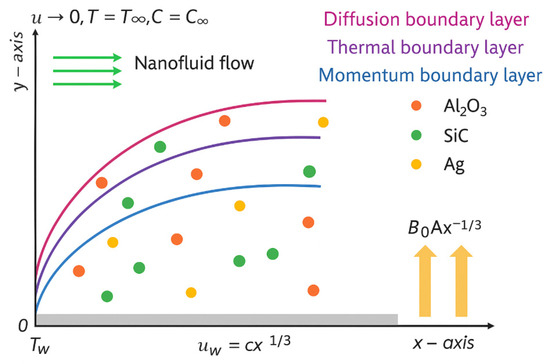
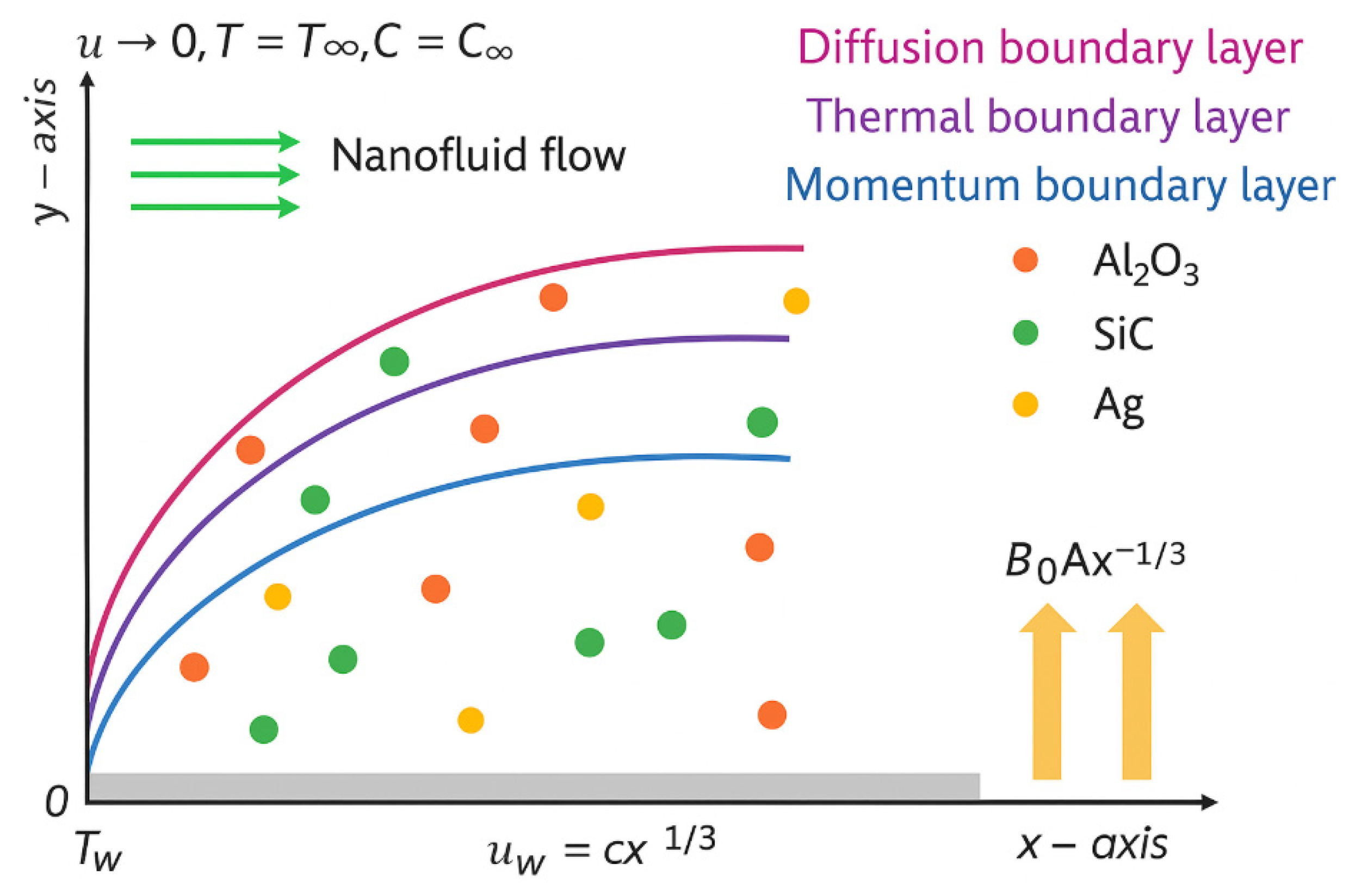
This paper uses a two-dimensional MHD CY-TNF model in order to find the flow of fluid over a sheet of stretched material with a velocity at a moving wall, as an analysis for enhancement of heat transfer $U_w$. This sheet has an uneven wall temperature $T_w$ and an inhomogeneous wall concentration $C_w$, with the outer environment sustaining a concentration $C_{\infty }$ and temperature $T_{\infty }$. The setup of Figure 1 is described as an irregular magnetic field $B$ applied to the fluid, which exhibits electrical conductivity. It thus can modulate fluid flow because the magnetic fluid interacts with an externally imposed magnetic field, further to promote or potentially cause an increase in the extent of heat transfer across it by altering flow and associated temperature distribution along its material surface.

Figure 1. Graphical configuration.

A unique mass and heat flux theory may be used to predict mass diffusion and heat energy transfer. It considers the dissipation of Joule heating. Moreover, tri-hybrid nanoparticles ($SiC, A{l}_2{O}_3, Ag$) are investigated in the base fluid ethylene glycol ($C_2{H}_6{O}_2$) during the heat flow via a permeable stretched sheet [25]. Thermal generation of energy caused by the interaction between a fluid that conducts electricity and a magnetic field is called Joule heating.

2.2. Governing Equation

$$u_x+v_y=0$$

(1)

$${\displaystyle \frac{{\rho }_{tnf}}{{\mu }_{tnf}}}\left(u{u}_x+v{u}_y\right)=u_{yy}{\left[1+\left(d+1\right){\left(\Gamma u_y\right)}^d\right]}^{{\displaystyle \frac{n-1}{d}}}-{\displaystyle \frac{{\sigma }_{tnf}}{{\mu }_{tnf}}}{B}_0^{2}A{x}^{-{\displaystyle \frac{2}{3}}}u$$

(2)

$$\begin{gathered} u{T}_x+v{T}_y={\displaystyle \frac{k_{tnf}}{{\left(\rho c_p\right)}_{tnf}}}{T}_{yy}+{\displaystyle \frac{{\sigma }_{tnf}}{{\left(\rho c_p\right)}_{tnf}}}{B}_0^{2}A{x}^{-{\displaystyle \frac{2}{3}}}{u}^2-\lambda (u_x{T}_x+v{v}_y{T}_y+u{v}_x{T}_y+v{u}_y{T}_x+2uv{T}_{xy}+u^2{T}_{xx} \\ +v^2{T}_{yy}-{\sigma }_{tnf}(2uv{u}_y+2u^2{u}_x)B_0^2{c}^{2}A{x}^{-{\displaystyle \frac{2}{3}}}\hspace{1em}\hspace{1em}\hspace{1em}\hspace{1em}\hspace{1em}\hspace{1em}\hspace{1em}\hspace{1em}\hspace{1em} \end{gathered}$$

(3)

$$u{C}_x+v{C}_y={\displaystyle \frac{D_{tnf}}{D_f}}{C}_{yy}-{\lambda }_c({uu}_x{C}_x+v{v}_y{C}_y+u{v}_x{C}_y+v{u}_y{C}_x+2uv{C}_{xy}+u^2{C}_{xx}+v^2{C}_{yy}$$

(4)

where $[u, v, 0]$ is the representation of the velocity component. The boundary conditions are as follows:

$$\begin{array}{c}u\left(0\right)=c{x}^{{\displaystyle \frac{1}{3}}} ,v\left(0\right)=0,T\left(0\right)=T_w, C\left(0\right)=C_w\hfill \\ u\left(\infty \right)=v\left(\infty \right)=0,T\left(\infty \right)=T_{\infty }, C\left(\infty \right)=C_{\infty }\hfill \end{array}$$

(5)

2.3. Similarity Transformation

The similarity variables [25]

$$\begin{array}{c}u=c{x}^p{f}^{\prime }\left(\eta \right), v=\sqrt{{\nu }_{fluid}c} x^{{\displaystyle \frac{p-1}{2}}} \left[{\displaystyle \frac{p+1}{2}}f+{\displaystyle \frac{p-1}{2}} \eta f^{\prime }\right]\hfill \\ \eta =y\sqrt{{\displaystyle \frac{c}{{\nu }_{fluid}}} }{x}^{{\displaystyle \frac{p-1}{2}}} , \theta \left(\eta \right)={\displaystyle \frac{T-T_{\infty }}{T_w-T_{\infty }}}, \phi \left(\eta \right)={\displaystyle \frac{C-C_{\infty }}{C_w-C_{\infty }}}\hfill \end{array}$$

for $p ={\displaystyle \frac{1}{3}}$ is used to convert Equations (1)–(5) into dimensionless form is

$$\begin{gathered} u=c{x}^{{\displaystyle \frac{1}{3}}}{f}^{\prime }\left(\eta \right), v=-{\displaystyle \frac{2}{3}}\sqrt{{\nu }_{fluid}c}{\displaystyle \frac{1}{x^{\frac{1}{3}}}}f+{\displaystyle \frac{1}{3}}\eta \sqrt{{\nu }_{fluid}c}{\displaystyle \frac{1}{x^{\frac{1}{3}}}}{f}^{\prime }, \eta =y\sqrt{{\displaystyle \frac{c}{{\nu }_{fluid}}}}{x}^{-{\displaystyle \frac{1}{3}}} \\ \theta \left(\eta \right)={\displaystyle \frac{T-T_{\infty }}{T_w-T_{\infty }}}, \phi \left(\eta \right)={\displaystyle \frac{C-C_{\infty }}{C_w-C_{\infty }}} \end{gathered}$$

(6)

2.4. Required ODEs

Hence one can get [25]

$$\begin{array}{c}{\displaystyle \frac{{(1-\overline{{\phi }_2})}^{2.5} }{{(1-\overline{{\phi }_1})}^{2.5}{(1-\overline{{\phi }_3})}^{2.5}}} f^{‴}\left[1+\left(d+1\right)\left(\left(n-1\right)d^{-1}\right)W{e}^d {\left(f^{″}\right)}^d\right]-{\displaystyle \frac{{\sigma }_{tnf}}{{\sigma }_{fluid}}} Ha{f}^{\prime }+{\displaystyle \frac{1}{3}}{\displaystyle \frac{{\rho }_{tnf}}{{\rho }_{fluid}}}\left[2f{f}^{″}-{f^{\prime }}^2\right]=0,\\ f\left(0\right)=0, f^{\prime }\left(0\right)=1,f^{\prime }(\infty )=0\end{array}$$

(7)

$$\begin{array}{c}{\displaystyle \frac{k_{tnf}}{k_{fluid}}}{\theta }^{″}+{\displaystyle \frac{{\sigma }_{tnf}}{{\sigma }_{fluid}}}HaPr Ec{f^{\prime }}^2+Pr{\displaystyle \frac{{\left(\rho c_p\right)}_{tnf}}{{\left(\rho c_p\right)}_{fluid}}}\hfill \\ \left({\displaystyle \frac{2}{3}}f{\theta }^{\prime }-\Delta \left[{\displaystyle \frac{2}{9}}{f}^{\prime }{f}^{″}{\theta }^{\prime }-{\displaystyle \frac{4}{27}}\eta f{f}^{″}{\theta }^{\prime }+{\displaystyle \frac{4}{9}}{f}^2{\theta }^{″}-{\displaystyle \frac{{\sigma }_{tnf}}{{\sigma }_{fluid}}} HaEc\left({\displaystyle \frac{4}{3}}f{f}^{\prime }{f}^{″}-{\displaystyle \frac{2}{3}}{f^{\prime }}^3\right)\right]\right)=0,\hfill \\ \theta \left(0\right)=1,\theta (\infty )=0\hfill \end{array}$$

(8)

$$\begin{array}{c}{\displaystyle \frac{D_{tnf}}{D_{fluid}}}{\phi }^{"}+Sc\left({\displaystyle \frac{2}{3}}f{\phi }^{\prime }-{\delta }_c\left[{\displaystyle \frac{2}{9}}f{f}^{″}{\phi }^{\prime }-{\displaystyle \frac{4}{27}}{\eta }^{2}f{f}^{″}{\phi }^{\prime }+{\displaystyle \frac{4}{9}}{f}^2{\phi }^{″}\right]\right)\hfill \\ \phi \left(0\right)=1,\phi (\infty )=0\hfill \end{array}$$

(9)

The parameters used in the equations above are:

$$\begin{gathered} We=c\sqrt{{\displaystyle \frac{c}{{\nu }_{fluid}}}}\Gamma , Ha={\displaystyle \frac{{\sigma }_{fluid}{B}_0^2{A}^2}{{\rho }_{fluid}c}}, Pr={\displaystyle \frac{{\left(\mu c_p\right)}_{fluid}}{k_{fluid}}},\hspace{1em}\hspace{1em}Ec={\displaystyle \frac{c}{{\left(c_p\right)}_{fluid}B{T}_0}}, \\ \Delta =c\lambda , Sc= {\displaystyle \frac{{\nu }_{fluid}}{D_{fluid}}},{\delta }_c=c{\lambda }_c\hspace{1em}\hspace{1em}\hspace{1em}\hspace{1em}\hspace{1em}\hspace{1em} \end{gathered}$$

Dimensionless quantities involved in the transformed governing equations have valuable physical information about the transport behavior of the non-Newtonian tri-hybrid nanofluid system. Hartmann number (Ha) is used to compare the electromagnetic force (due to the application of a magnetic field) and viscous force acting on the fluid, and to describe how strongly the applied magnetic field is able to influence the motion of the fluid. Increasing values of Ha will increase the magnitude of the Lorentz force dampening effect, thereby decreasing the velocity field and increasing the amount of thermal energy that accumulates within the fluid. The Weissenberg number is a measure of the elasticity of these fluids and is regarded as the ratio of elastic relaxation influence to viscous forces between fluids in motion. As the Weissenberg number increases, it has been established that the level of viscoelasticity in a fluid increases, as well as the characteristics of momentum transport within the boundary layer. The Eckert number is used to quantify the viscous dissipation of energy in the fluid, or the conversion of kinetic energy into internal thermal energy, as a result of fluid friction. The magnitude of the Eckert number determines the temperature of the fluid; as the Eckert number increases, the amount of thermal energy generated by the fluid increases as well, thus increasing the temperature of the fluid in the system. The Prandtl number indicates the ratio of the diffusivity of the momentum and the thermal diffusivity between fluids in motion. An increase in the Prandtl reduces thermal diffusion and, as a result, reduces the thickness of the thermal boundary layer. The Schmidt number indicates the ratio of the momentum diffusivity to the mass diffusivity of the fluid, which has a governing effect on the concentration transport through the fluid. As the Schmidt Number increases, mass diffusion is reduced, resulting in a reduced thickness of the concentration boundary layer. The thermal relaxation parameter measures finite-speed propagation of heat, and this is due to the use of the Cattaneo–Christov heat flux model; the solutal relaxation parameter measures delayed diffusion of mass.

3. Construction of ANN-Based LBMT Solver

The three components of the approach are included in this section. First, the data set will be created using the bvp4c numerical approach. Next, ANN-LM will be formulated, and lastly, the performance indices will be discussed. To resolve the problem of the governing boundary value of the mathematics model of the CCHMF–THNF, we used a hybrid method based on MATLAB’s bvp4c solver and the ANN–LM optimization process. The numerical procedure is comprised of three main stages, which include: (1) dataset generation, (2) ANN training/validation, and (3) convergence testing.

• Dataset Generation using bvp4c:

• Discretization of the governing nonlinear ODE system using a finite-difference collocation method in MATLAB’s bvp4c.
• The solution was calculated iteratively until the residual tolerance approached ${10}^{-8}$.
• The dataset created will be obtained velocity, temperature and concentration profiles at the different Weissenberg number (We), Hartmann number (Ha), thermal relaxation parameter (Δ) and solutal relaxation parameter (λ) values.

• Preparation of ANN Training Data:

• Input variables: [$We,Ha,\Delta ,\lambda$].
• Output variables: velocity, temperature, concentration.
• The data was split into 70% training, 15% validation, and 15% testing.
• All data is normalized in the range of [0, 1] for constant and stable learning.

• ANN–LM Training and Convergence Criteria:

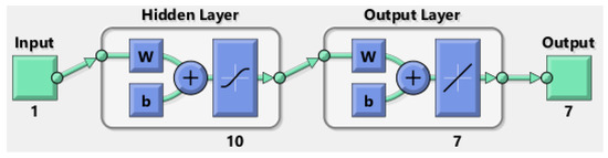
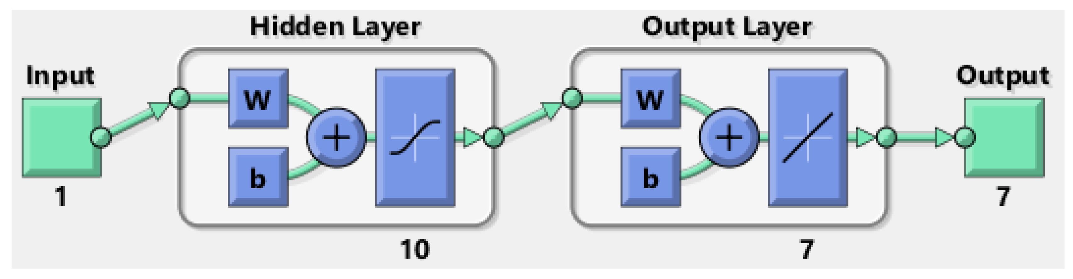
• The ANN design has a hidden layer with 10 neurons and log-sigmoid activation functions.
• Training was performed with the Levenberg–Marquardt backpropagation algorithm.
• Convergence was reached when:

  ▪

  a mean square error (MSE) of less than ${10}^{-10}$ was reached;

  ▪

  validation error did not increase for more than 10 consecutive epochs; and

  ▪

  training stopped before reaching the maximum of 1000 epochs if none of the previous conditions were met.

• Regression analysis, error histograms, and fitness curves were used to confirm convergence and ensure that overfitting did not occur.

Our suggested work steps are illustrated in Algorithm 1.

Algorithm 1: Proposed Methodology

(a) Define the equations and boundary conditions that govern the dimensionless system. (b) Numerically generate reference solutions using bvp4c in MATLAB. (c) Create the dataset by varying the governing parameters over the allowed range. (d) Split the resulting dataset into 70% for training, 15% for validation, and 15% for testing. (e) Initialize an artificial neural network (ANN) with 1 hidden layer and a log-sigmoid activation function. (f) Train the ANN with the Levenberg–Marquardt optimization algorithm. (g) Use mean squared error, root mean squared error, mean absolute error, and regression analysis to quantify the accuracy of ANN predictions. (h) Compare the ANN’s predictions to those of the target data generated with bvp4c. (i) Perform a parametric analysis of the velocity, temperature, and concentration profiles.

This section describes the two-step computational framework that combines AI with ANN-LM. Figure 2 shows the network capabilities based on the multi-layer. The “nfool” (built-in MATLAB), “validation by cross” (n-folded), “function of activation” (log-sigmoid), “epochs” (maximum 1000), ranges (${10}^{-7}$), “step size” (0.01), “hidden layers” (ten neurones), “algorithm” (LBMT), and “layers” (output/hidden/input) are used to provide the AI and the ANN-LM processes for the language-based model. The fundamental outputs are used to get the label static information using the input/target performance during training.

Figure 2. Single-layer neuron structure.

The design of neural networks involves many key aspects, such as defining the framework, specifying the cost function, choosing the function for activation, and then training the model. Incorporating scaling into this process may require taking into account regularization, weight initialization, and input topographies. The following are some of the general structure’s phases for constructing neural networks with scalability in mind:

• Explanation of the problem: By choosing the kind of data and value ranges for the input parameter space, the language learning model is used to define the problem through the regression process.
• Preprocessing the data: Normalize or standardize the input topographies to a comparable measurement. Preprocessing the data gives the model the assistance it needs to converge more quickly during training, improving performance.
• Architecture design: The neural network design based on the types and quantity of layers is detailed, using various levels of normalization to enable an internal covariate data, a shift that is relevant to scaling.
• Weight initialization: To initialize the weights, choose a suitable scheme. The weights have been carefully and thoughtfully chosen.
• Activation functions: The log-sigmoid function, which is used in this work and is displayed in Figure 3 during the hidden layer procedure, is the specifically selected activation function.
• Loss function: The mean square error (MSE) for regression is used to choose this function.
• Optimization: The ANN-LM is used to carry out the optimization.
• Training: The model is trained using the data in order to monitor the performance utilizing the authentication sets.
• Model evaluation: The model’s generalization presentation is measured via a series of independent tests.

Figure 3. ANN-LM topology.

Taking everything into account regarding the evaluation of advantages and disadvantages concerning the ANN-LM scheme, it has been considered for some key aspects. There is the aspect of moderate approximation of the problem solution, then there is the stable and rapid convergence toward the results, and lastly, the computational efficiency of the scheme plays a vital role in evaluating the numerical methods, mainly when dealing with large-scale problems. This feature of handling divergent input data formats also constitutes an important factor of the method, whereby adaptability is maintained across various applications. All these factors may together yield a holistic view of the strengths and possible limitations of the ANN-LM scheme.

A computational stochastic AI, integrated with the ANN-LM solver, has been applied to solve the differential model learning language using ten neurons. It has been verified by checking its performance through optimal handling of under-fitting and overfitting as obtained with a training and corroboration process over a maximum of 1000 epochs. The under-fitting, or early convergence, occurs for low neuron counts, and overfitting, with higher complexity and possibly lower generalization, is traced with a larger count of neurons. The labeling data of the model, trained on measures of input, training, and target, are monitored using simple output distribution across testing at 15%, validation at 15%, and training at 70% ratios to solve the nonlinear fluidic differential model effectively. The computational values for the input range [0, 1] that are obtained by the stochastic AI and ANN-LM solver validate the solution to the fluidic differential model further.

3.1. Sensitivity Analysis of ANN Parameters

To optimize the ANN–LM solver, we conducted a comprehensive sensitivity analysis focusing on a single hidden layer architecture. The analysis examined: (1) number of neurons, (2) activation functions, (3) training algorithms, and (4) data splitting ratios.

3.1.1. Neuron Count Sensitivity

We tested neuron counts from 5 to 40 while keeping other parameters constant (log-sigmoid activation, LM algorithm, 70/15/15 split). Results are summarized in Table 1.

Table 1. Effect of neuron count on single-layer ANN performance.

Neurons	Training MSE	Validation MSE	Testing MSE	Training Time (s)	Convergence Epochs	Status
5	4.21 × 10−8	6.85 × 10−8	5.92 × 10−8	0.6	95	Underfit
8	1.82 × 10−9	2.45 × 10−9	3.12 × 10−9	0.8	112	Good
10	8.53 × 10−11	1.08 × 10−10	1.21 × 10−10	1.2	125	Optimal
15	6.24 × 10−11	9.87 × 10−11	1.05 × 10−10	1.8	143	Good
20	5.12 × 10−11	8.35 × 10−11	9.24 × 10−11	2.4	156	Good
25	4.98 × 10−11	8.12 × 10−11	8.95 × 10−11	3.1	168	Marginal gain
30	4.87 × 10−11	1.24 × 10−10	1.85 × 10−10	4.0	185	Overfit
35	3.95 × 10−11	2.15 × 10−10	2.98 × 10−10	5.2	210	Overfit
40	3.12 × 10−11	3.85 × 10−10	4.12 × 10−10	6.8	235	Severe overfit

The key observations of Table 1 are:

• Optimal range: 10–20 neurons
• Sweet spot: 10 neurons (best generalization)
• Underfitting: <8 neurons (MSE > 10⁻⁸)
• Overfitting: >25 neurons (validation MSE increases)

3.1.2. Activation Function Comparison (10 Neurons)

Table 2 shows that log-sigmoid provides the best convergence due to its smooth, bounded output (0,1), which matches our normalized data range and facilitates gradient-based optimization.

Table 2. Activation function performance for single hidden layer (10 neurons).

Activation	Training MSE	Validation MSE	Epochs	Gradient	μ Parameter	Remarks
Log-sigmoid	8.53 × 10−11	1.08 × 10−10	125	9.97 × 10−9	1.0 × 10−9	Best
Tanh	1.42 × 10−10	1.95 × 10−10	108	8.45 × 10−9	1.0 × 10−9	Good
ReLU	5.82 × 10−8	8.15 × 10−8	285	1.24 × 10−7	1.0 × 10−8	Poor
Linear	2.15 × 10−7	3.42 × 10−7	420	2.85 × 10−6	1.0 × 10−7	Worst

3.1.3. Training Algorithm Comparison

From Table 3 the Levenberg–Marquardt (LM) outperforms others due to its hybrid approach combining gradient descent and Gauss–Newton methods.

Table 3. Training algorithms for single-layer ANN (10 neurons, log-sigmoid).

Algorithm	Training MSE	Val. MSE	Epochs	Time (s)	Gradient
LM	8.53 × 10−11	1.08 × 10−10	125	1.2	9.97 × 10−9
BFGS	2.15 × 10−10	3.24 × 10−10	195	2.1	1.85 × 10−8
SCG	5.82 × 10−10	7.15 × 10−10	165	1.8	2.45 × 10−8
RP	1.24 × 10−9	1.85 × 10−9	280	2.8	4.12 × 10−8

3.1.4. Data Splitting Sensitivity

From Table 4 70/15/15 provides the best balance between training sufficiency and generalization testing.

Table 4. Effect of training/validation/testing ratios (10 neurons, LM).

Split Ratio (T/V/Te)	Training MSE	Validation MSE	Testing MSE	Generalization Error
60/20/20	7.25 × 10−11	1.42 × 10−10	1.85 × 10−10	2.15 × 10−10
70/15/15	8.53 × 10−11	1.08 × 10−10	1.21 × 10−10	1.15 × 10−10
80/10/10	5.12 × 10−11	2.85 × 10−10	3.24 × 10−10	3.05 × 10−10
50/25/25	9.85 × 10−11	1.65 × 10−10	2.15 × 10−10	1.90 × 10−10

As shown in Figure 3, the performance of the layers involved in solving the fluidic differential model is demonstrated.

The dataset used for ANN training consists of numerically converged solutions obtained from bvp4c under mesh-independent conditions. The input parameter space includes:

$$We\in [0.5, 2.5],Ha\in [0.5, 2.0],\Delta \in [0.1, 1.0],\lambda \in [0.1, 1.0]$$

A total of 1200 samples were generated and distributed as:

• Training: 840 samples
• Validation: 180 samples
• Testing: 180 samples

The ANN predictions were compared against numerical solutions presented in Table 5.

Table 5. Statistical analysis for ANN prediction.

Metric	Value
MSE	1.2 × 10−10
RMSE	3.4 × 10−6
MAE	2.1 × 10−6
R2	0.9992

These results confirm that the ANN model accurately reproduces the numerical dataset with negligible error.

In order to test temperature, velocity, and other flow parameters, the CCHMF-CYTNF design is solved using the proposed ANN-LM procedure, which is described in this section. The explanation of stochastic techniques is divided into two phases. The important features are first provided by the ANN-LM operator; in the second phase, the ANN-LM operator strategy is employed to carry out the intended CCHMF-CYTNF. The following are some special ANN-LM parameter spaces for resolving the planned CCHMF-CYTNF:

The framework may be successfully addressed using the stochastic measure computational ideas. The stochastic techniques are first used to give the solutions for the CCHMF-CYTNF system.

• A number of CCHMF-CYTNF system variables are displayed to confirm the reliability of the recommended fix.
• The ingenuity and effectiveness of the proposed stochastic computing ANN-LM solvers are demonstrated by comparing the results with the reference (bvp4c).
• The system is solved and the efficacy of ANN-LM solvers is assessed using the least absolute error (Ab.Er).

3.2. Mesh Independent Study

A mesh independence and solver tolerance analysis was performed on the numerical dataset used for training the ANN to ensure its accuracy. This was achieved using the MATLAB bvp4c solver to solve the governing nonlinear ODE system by solving the equations over a finite computational domain of $\eta \in [0,5]$ using different mesh densities. Table 6 shows the results of the mesh-independent analysis of the velocity, temperature, and concentration error.

Table 6. Mesh study.

Grid Points	Velocity Error	Temperature Error	Concentration Error
100	2.31 × 10−4	3.12 × 10−4	2.87 × 10−4
250	5.42 × 10−6	6.31 × 10−6	5.88 × 10−6
500	8.15 × 10−8	9.04 × 10−8	8.72 × 10−8
750	7.98 × 10−8	8.91 × 10−8	8.63 × 10−8
1000	7.96 × 10−8	8.89 × 10−8	8.60 × 10−8

When the grid points increased from 500, then it is observed that the variation becomes negligible, which confirms the mesh independence. Table 7 presents the tolerance sensitivity analysis.

Table 7. Tolerance sensitivity analysis.

Tolerance	Max Residual Error
10−3	1.25 × 10−3
10−5	4.38 × 10−6
10−6	7.21 × 10−8
10−7	8.03 × 10−8
10−8	7.99 × 10−8

The solution stabilizes for tolerance $\le {10}^{-6}$. Therefore, all simulations were conducted using ${10}^{-7}$ tolerance and 500 grid points.

These results confirm that the dataset used for ANN training is numerically converged, stable, and highly accurate.

4. Numerical Outcomes of CCHMF-CYTNF

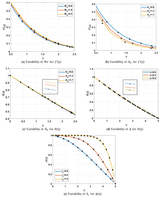
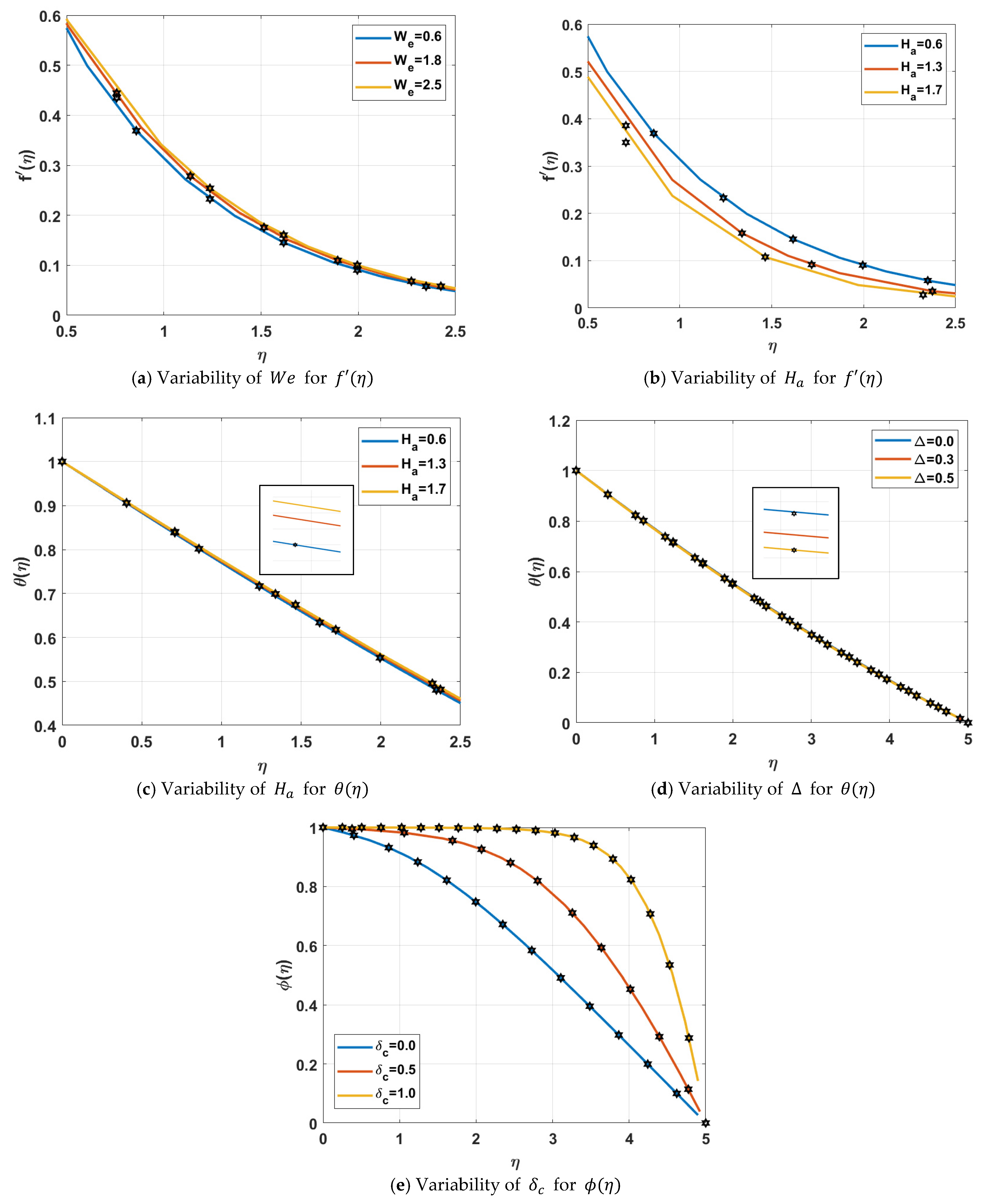
This figure and others in Figure 4a–e illustrate how the forces, fluid properties, and applied fields all interact with each other in complex ways to predict fluid flow behavior and temperature fields.

Figure 4. Evaluation of ANN-LM for $f^{\prime }\left(\eta \right)$, $\theta \left(\xi \right)$ and $\varphi$($\eta$) with reference dataset of CCHMF-CYTNF model.

4.1. Figure 4a: Dependency of Fluid Velocity on Weissenberg Number $We$

Figure 4a indicates that with an increase in the Weissenberg number, $We$, this means an increase in fluid velocity. The Weissenberg number is the ratio between elastic and viscous forces in the fluid. It gives a reflection of the relative strength in these forces. As $We$, elastic forces become more important than viscous forces, as the fluid accelerates. In this case, elastic forces are less restrictive than the viscous forces. So, the fluid moves quite freely. Therefore, it is with higher We value the idea that the fluid contains more elasticity than viscosity, with a rise in the velocity of the fluid.

4.2. Figure 4b: Variability of Velocity Trajectory with Hartmann Number (Ha)

Effect of Ha on velocity trajectory as illustrated in Figure 4b. For the case of Ha, the fluid velocity field decelerates as increases. In this effect, there is a Lorentz force attributed as a magnetic resistance force against the motion of the charged fluid particles. When a magnetic field is applied, the Lorentz force opposes the fluid’s movement, thereby reducing its velocity. That is why an increase in is considered a decelerating factor for the fluid’s velocity field. The Hartmann number gives the strength of the magnetic field, which indicates that more magnetic damping would be developed on fluid particles, hence slowing the flow of fluid.

4.3. Figure 4c: Variability of Temperature Profile with Hartmann Number, $\theta \left(\eta \right)$

In Figure 4c, the variability of the temperature profile, $\theta \left(\eta \right)$, is shown in relation to the change in the Ha values. With an increase in value of Ha, the temperature of the fluid increased. This is due to the electrical conductivity of the fluid and its ability to absorb energy from the applied magnetic field. Electrically conducting fluids generate electric currents when subjected to a magnetic field because the motion of fluid particles interferes with the magnetic lines of force. The generated electric currents undergo Ohmic dissipation, where electrical energy is converted into heat. This increased temperature, because of Ohmic dissipation, is distributed to the fluid particles.

The interaction of the applied magnetic field and the electrically conducting liquid creates a Lorentz force, enhanced with an increased Hartmann number, allowing an increase in amount of heat trapped within the thermal boundary layer due to the increase in magnetic resistance. This is as clear as seen in that when the Hartmann number increases from 0.6 to 1.7 by approximately 18–24%, it will produce increments in temperature found within those parameters. A similar thermally enhanced result due to magnetic effects was produced during previous work on MHD non-Newtonian nanofluids as well [25].

4.4. Figure 4d: Effect of Thermal Memory Parameter (Δ) on Temperature Profile

In Figure 4d, we examine the effect of the thermal memory parameter Δ on the temperature profile. The parameter Δ measures the fluid’s “memory” for past thermal states, and this memory has an influence on the mode of heat transfer between particles. The increase in Δ leads to a decrease in the rate of heat exchange between particles and their surroundings, which decreases the fluid temperature overall. That is to say, the more considerable this parameter is, that is to say, the larger, the more considerable the thermal memory effect becomes, and this phenomenon further lowers the dissipation rate of the released heat, which in turn lowers the temperature inside the fluid.

4.5. Figure 4e: Effect of Parameter ${\delta }_c$ on Concentration Profile of CCHMF-CYTNF

Figure 4e presents how the concentration profile of the CCHMF-CYTNF system varies with a variation in the parameter ${\delta }_c$. With increasing values of ${\delta }_c$, higher values of ${\delta }_c$ reduce mass diffusivity, thereby decreasing the concentration boundary layer thickness, and hence the concentration profile is low. This implies that for large ${\delta }_c$ the spreading rate of the particles through the material is less, and therefore the concentration is less.

4.6. Figure 5a–e: Absolute Error Analysis for Validation

The absolute errors that occurred in the model prediction are presented in Figure 5a–e. Small absolute errors in all the cases from the ANN-LM result confirm the validity of the proposed method. The CCHMF-CYTNF model’s insignificant absolute error was calculated for each of the situations between ${10}^{-2}$ and ${10}^{-8}$. Low error values indicated the accuracy of the model in predicting fluid flow, thermal, and concentration profiles and thus proved to be reliable in giving accurate and consistent results. This very high accuracy in such a scenario once again revalidates the validity and precision of this model and indicates that this method indeed appropriately mimics fluid behavior at many parameter alterations. In essence, all these observations capture the subtle interplay of elastic, viscous, and magnetic forces together with thermal and concentration dynamics that make the model itself so effective for predicting complex behaviors of fluids.

Figure 5. Absolute error (Abs-Er) for $f^{\prime }$ ($\mathsf{\eta }$), $\theta \left(\xi \right)$ and $\varphi$($\mathsf{\eta }$) with reference dataset of CCHMF-CYTNF model.

Figure 5. Absolute error (Abs-Er) for $f^{\prime }$ ($\mathsf{\eta }$), $\theta \left(\xi \right)$ and $\varphi$($\mathsf{\eta }$) with reference dataset of CCHMF-CYTNF model.

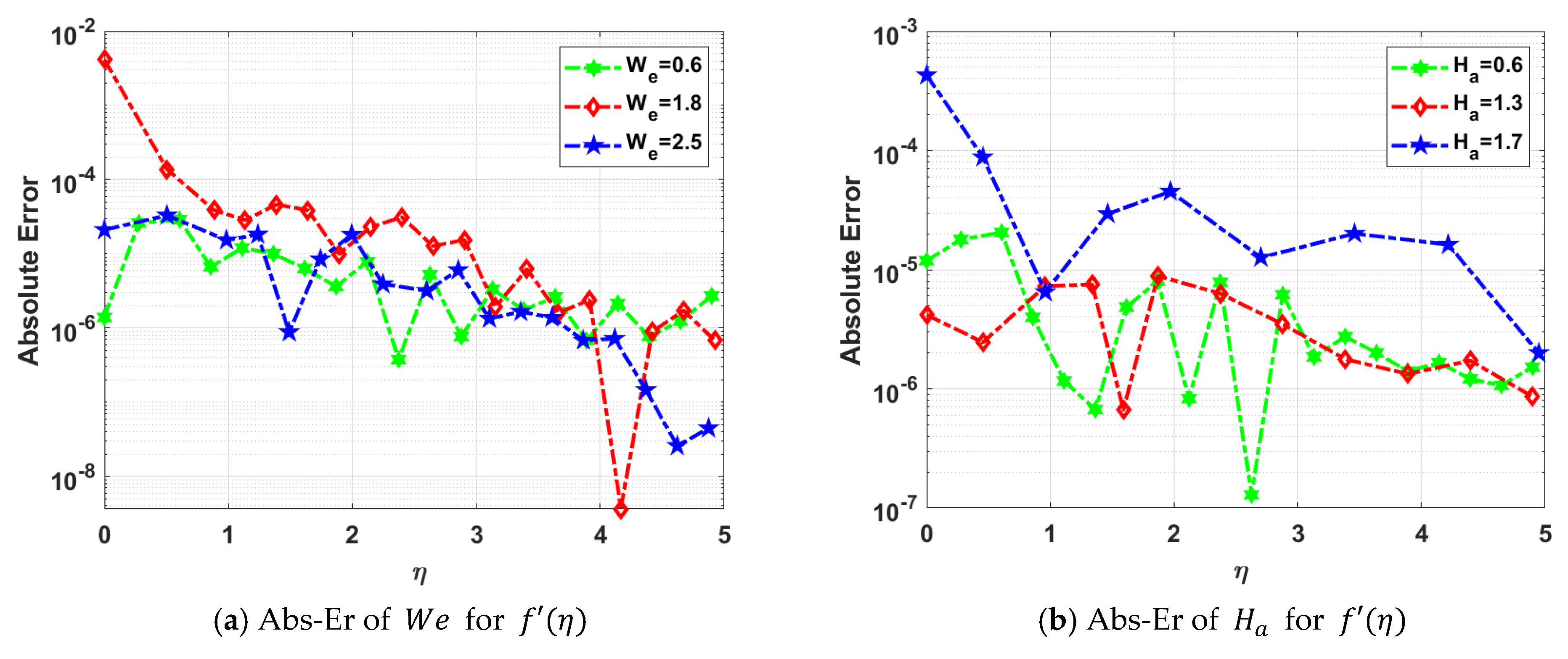
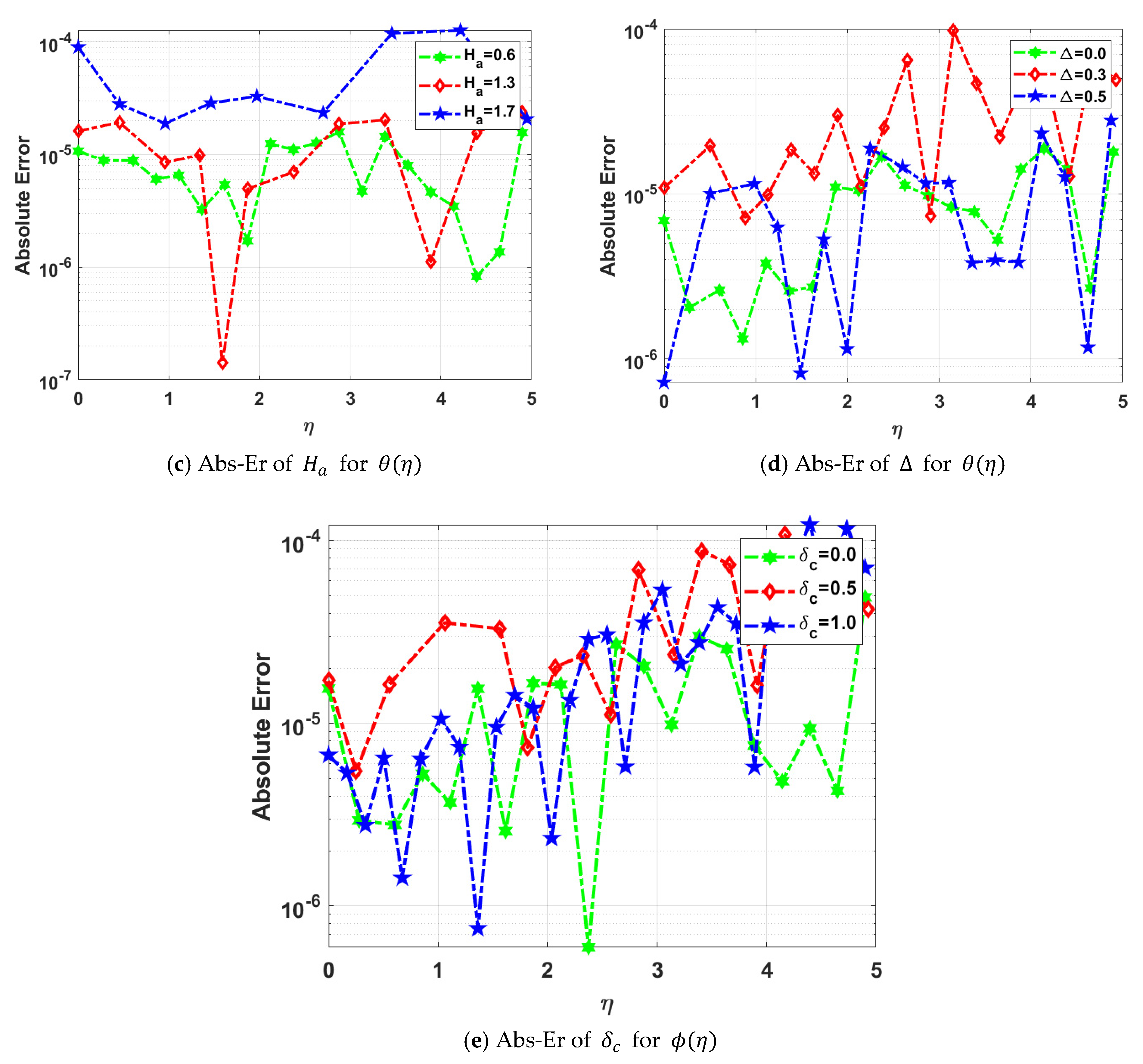
The combined effects of the Weissenberg and Hartmann numbers show different transport characteristics when compared to changing just one of the individual parameters. When the Weissenberg number is increased, the fluid experiences more elastic behavior (Carreau–Yasuda fluid), which allows for higher momentum transfer and an increase in the velocity. Conversely, increasing the Hartmann number results in a higher Lorentz force being produced by the magnetic field, which will act to inhibit the motion of the fluid due to the increase in magnetic damping. The results from this study indicate that there is an interaction between the elastic effect being enhanced by the presence of a magnetic field and the fluid’s resistance due to that same magnetic field. Therefore, the results would show different levels of performance through interpolation of two independent parameters. At lower values of the Hartmann number (Ha < 1), the elastic properties of the fluid will dominate the momentum transfer and the velocity profile will increase significantly with an increase in the Weissenberg number. However, as the magnetic strength increases (Ha > 1.5), the effect of the Lorentz force on damping will dominate and will progressively inhibit the elastic effects. From a quantitative perspective, an increase in the Weissenberg number from 0.6 to 2.5 produced approximately a 21% increase in peak velocity, while the increase from 0.6 to 1.7 in the Hartmann number produced an approximate decrease of 28% in peak velocity for the same conditions represented in this investigation. These results demonstrate a gradual transition from an elasticity-dominated transport regime to one controlled by the effect of the magnetic field with increasing magnetic field strength. The physical consistency of the obtained numerical results further supports the accuracy of the computational model as demonstrated by its behavior as the governing parameters approach their limits. When Ha→0, the contribution of the magnetic field completely disappears. Hence, the governing equations reduce to those for a non-Newtonian, incompressible fluid flowing without a Lorentz force. When the Lorentz force diminishes, the velocity profile develops layers of shear along the flow direction that are gradually increasing in strength relative to the absence of that force, while the thermal field reduces in strength since the contributions due to Joule heating will also diminish. In the opposite limit of We→0, the effect of elastic forces on the fluid behavior will be negligible and the fluid will resemble a near-Newtonian condition dominated by viscous forces, where the velocity gradients will be smooth and the momentum boundary layer will be significantly thinner than when there are viscoelastic properties present in the fluid. In addition, higher values of thermal relaxation parameters will impede the propagation of heat as a result of the gradual delay in thermal response associated with the Cattaneo–Christov model, while larger solutal relaxation parameters will impede the dissipation of concentration as well as reduce the concentration boundary layer thickness. When Ha decreased from 1.7 to 0, there was an enhancement in peak flow velocity measurement of about 31%, confirming the significant influence of magnetic damping on momentum suppression. In addition, decreasing We toward 0 also reduces elastic transport effects and results in flow behavior consistent with conventional viscous fluid dynamics. These limiting-case descriptions establish that the numerical predictions produce expected physical responses based on numerically matching the asymptotic parameters and demonstrate the validity of the numerical analysis.

Table 8 presents the non-variable outcomes of ANN-LM, with a focus on gradient values, significant performance metrics, and the training mu. Considering the length of each epoch and the overall number of epochs required for convergence, these results provide insight into the computing efficiency. By examining these factors, the table illustrates how the performance of the ANN-LM model varies throughout training.

Table 8. Outcomes of ANN-LM.

Scenario	Case	Mean Squared Error			Performance	Mu Parameter	Gradient	Epochs	Time
		Training	Validation	Testing
SCE-I	I	1.22834 × 10−10	2.85390 × 10−10	6.37201 × 10−10	1.23 × 10−10	1.00 × 10−9	9.97 × 10−9	125	1 s
	II	1.67531 × 10−9	2.38132 × 10−7	2.94329 × 10−9	1.68 × 10−9	1.00 × 10−8	9.98 × 10−8	150	0 s
	III	1.99571 × 10−10	1.15624 × 10−9	2.15049 × 10−10	1.72 × 10−10	1.00 × 10−9	2.35 × 10−7	81	0 s
SCE-II	I	9.99439 × 10−11	1.03809 × 10−10	1.21392 × 10−10	9.99 × 10−11	1.00 × 10−9	9.86 × 10−8	213	1 s
	II	8.53663 × 10−11	1.08270 × 10−10	4.09254 × 10−9	8.54 × 10−11	1.00 × 10−9	9.94 × 10−8	233	1 s
	III	1.41469 × 10−9	2.15742 × 10−9	1.21911 × 10−8	1.41 × 10−9	1.00 × 10−8	9.97 × 10−8	307	1 s
SCE-III	I	1.02509 × 10−10	1.04248 × 10−10	1.02236 × 10−10	1.03 × 10−10	1.00 × 10−9	9.88 × 10−8	144	0 s
	II	2.15825 × 10−9	3.02879 × 10−9	7.49342 × 10−9	2.16 × 10−9	1.00 × 10−8	9.91 × 10−8	154	99 s
	III	1.24246 × 10−10	3.52427 × 10−10	2.41013 × 10−10	1.24 × 10−10	1.00 × 10−9	9.94 × 10−8	120	0 s
SCE-IV	I	1.34399 × 10−9	3.00395 × 10−9	4.23060 × 10−8	1.34 × 10−9	1.00 × 10−8	9.98 × 10−8	176	1 s
	II	2.22191 × 10−10	2.39220 × 10−10	2.93778 × 10−10	2.22 × 10−10	1.00 × 10−9	1.00 × 10−7	112	0 s
	III	1.31074 × 10−9	2.13042 × 10−9	3.10711 × 10−8	1.42 × 10−9	1.00 × 10−8	9.97 × 10−8	183	1 s

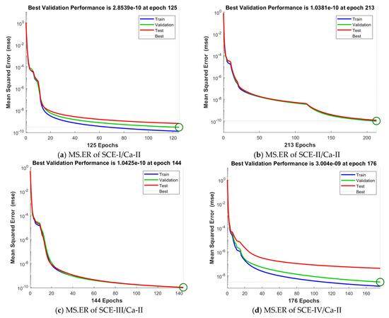
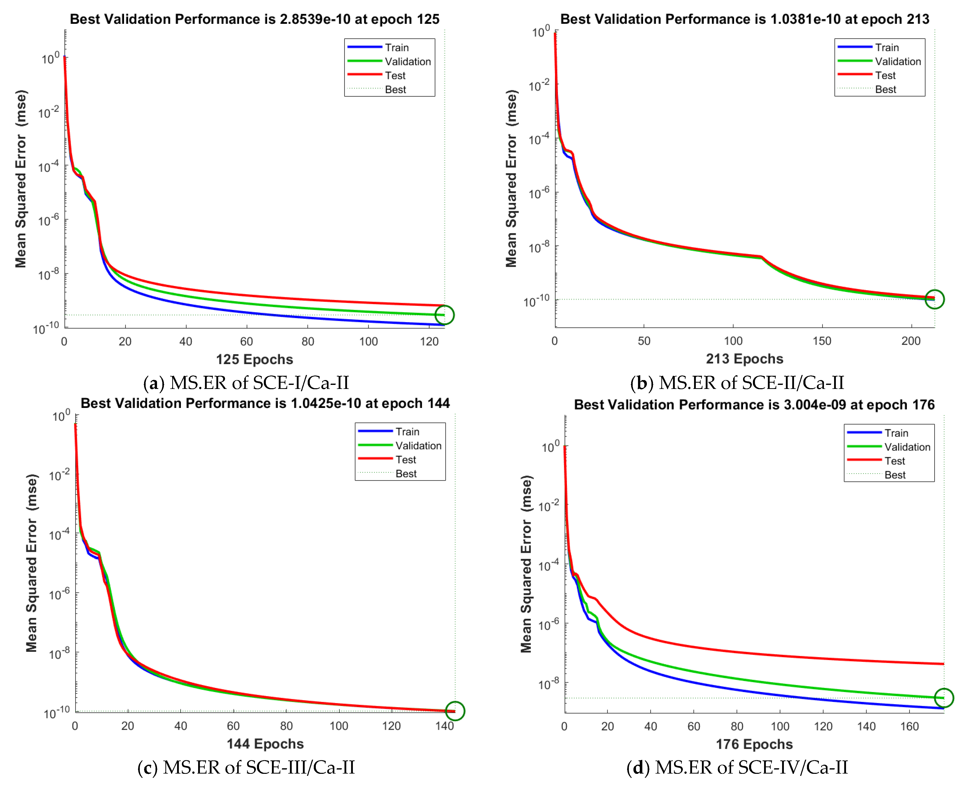
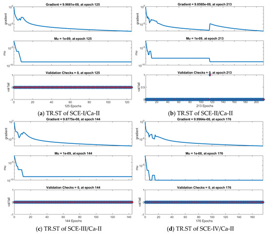
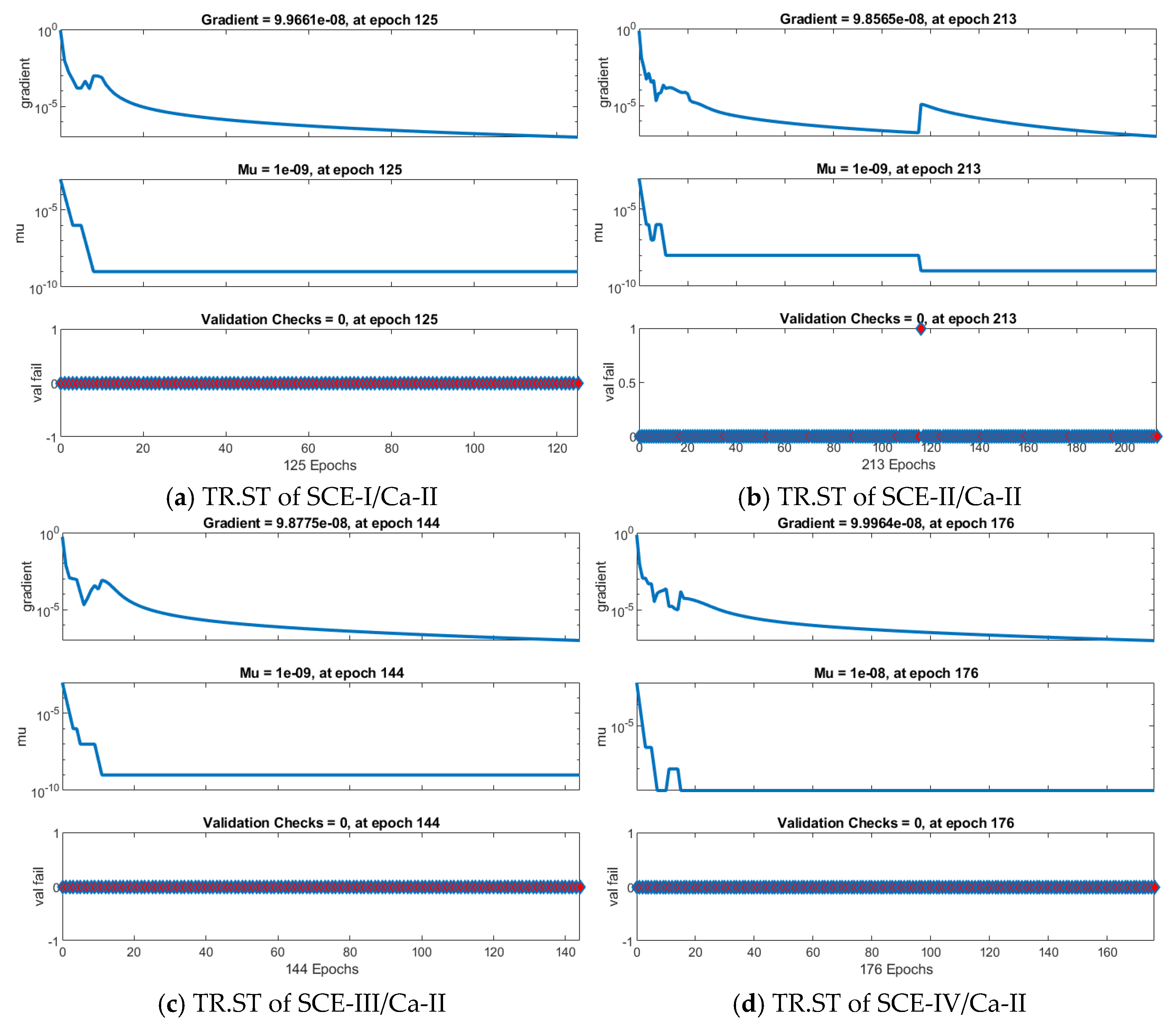
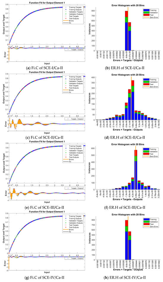
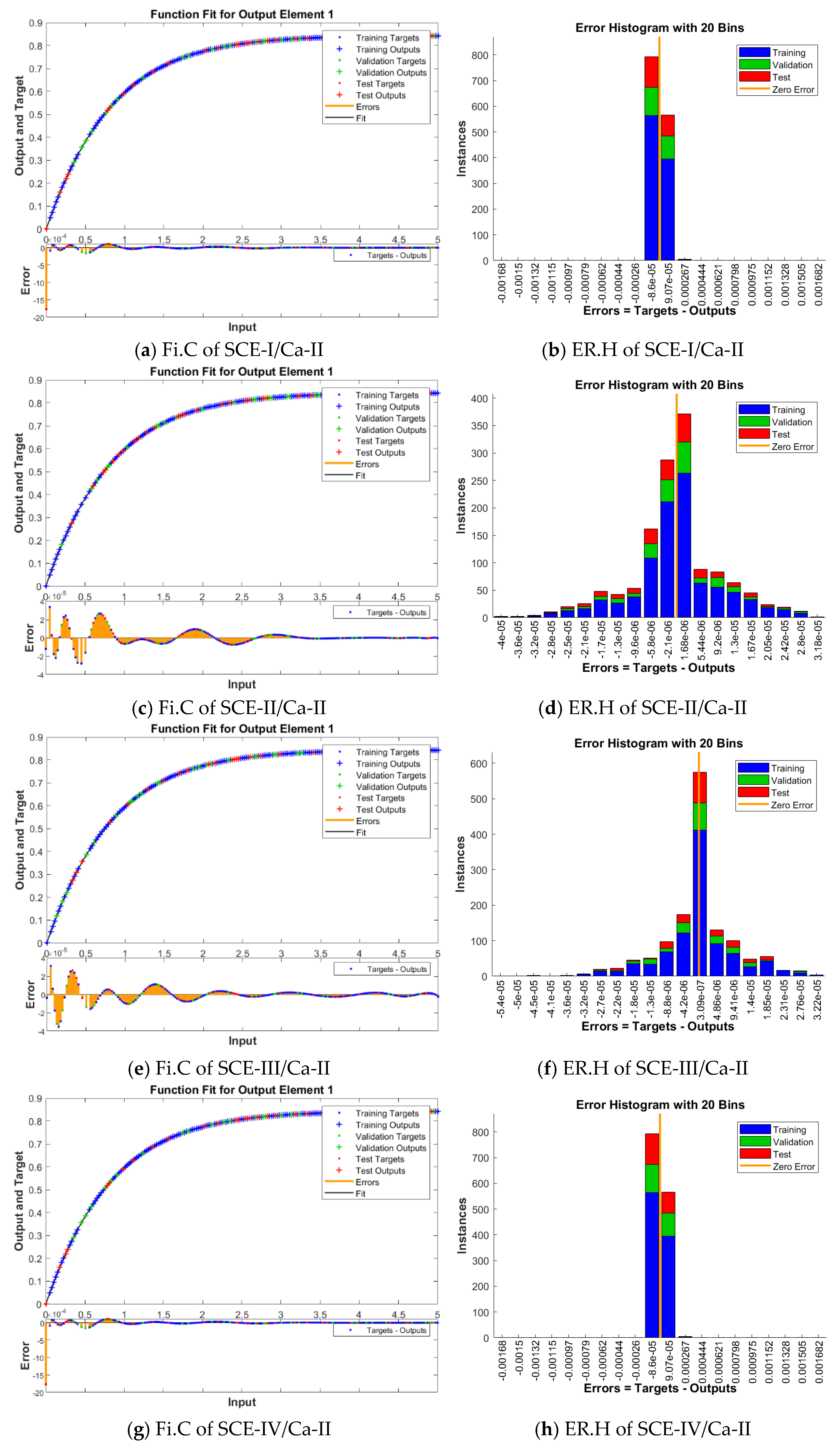
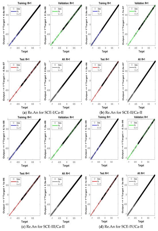
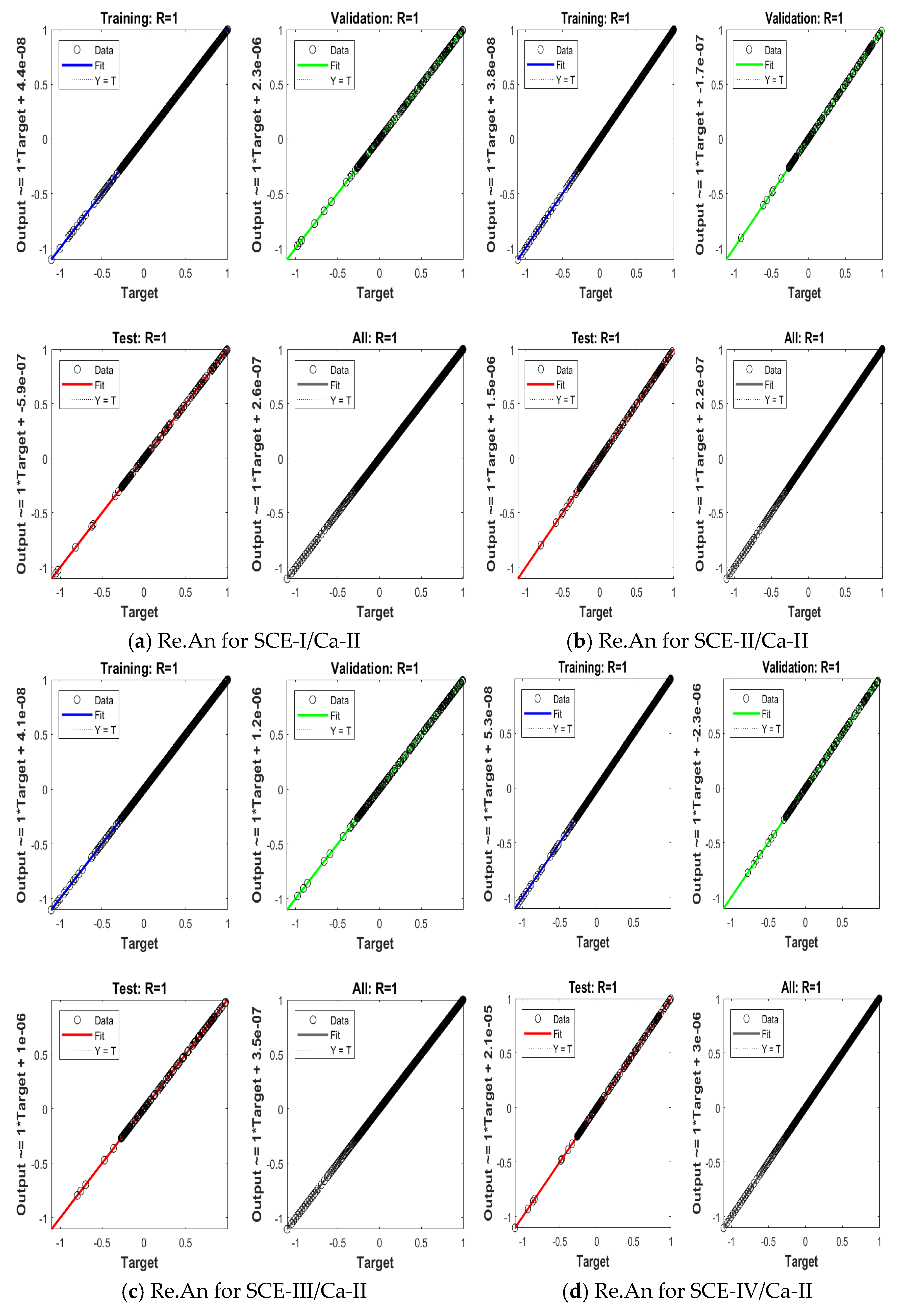
Figure 6a–d with CCHMF-CYTNF (I-IV) display the suggested ANN-LM for merging training usefulness and evaluating advancements against epochs grade for handling case I of the scenario. MSEs are found at 125, 213, 144, and 176 epochs, respectively, and are around 2.854 × 10⁻¹⁰, 1.038 × 10⁻¹⁰, 1.042 × 10⁻¹⁰, and 3.00 × 10⁻⁹. The MSE loss function is often used in neural networks to determine the difference between predicted and actual output values. It calculates the overall difference between the network’s projected values and the actual target values. “trainFcn” is the name of the neural network’s training function. The assumption that LMBN operates well and efficiently is further supported by the lines that arise from these epochs, which converge uniformly, signifying the achievement of the equilibrium point. This remark is important since it shows a consistent and reliable attitude across the computational performance. The model’s ability to get better results, as indicated by decreasing MSE values, is highlighted by the performance evaluation, which is shown in Table 5 as well as the corresponding figures. The notion that a decrease in MSE signifies improved efficacy and accuracy of the LMBN approach is supported by the fact that outcomes and MSE values have an inverse relationship. This finding supports the theory that improved model correctness is indicated by lower mean squared error (MSE) values. The best stability and performance are shown by an uninterrupted development. Lower MSE values suggest increased performance accuracy, as seen in Table 5. In the study, the low MSEs are due to how the numerical data was generated using MATLAB’s bvp4c solver. The data has no experimental noise or measurement uncertainty; therefore, prediction errors are small when using the ANN-LM framework to approximate nonlinear numerical solutions. It should be noted that this work only intends to evaluate how well the ANN-LM reproduces the numerical target data generated by bvp4c, not to evaluate the ANN-LM for the generalization of the existing experimental applications. Therefore, this framework is a computer-based approximation model for nonlinear numerical datasets. The present study only employed independent training, validation and test subsets to help reduce overfitting. Quantifying uncertainty in the model, adding noise to the outputs and robustness analyses of the model against experimental variability are not included in the present study. These additional areas would provide future directions as they relate to enhancing the generalization and applicability of the model. The convergence efficiency, homogeneity, and dependability for handling case I of the simulator (I–IV) in CCHMF-CYTNF are shown in Figure 7a–d, where Mu stands for gradient and phase margin. The gradient is a generalization of the derivative, which is a multidimensional function. Since a small step from such a position preserves the localized slope of the function, we can predict the result in any direction. Training will become quite modest as it gets closer to the performance obstruction. Mu is the regulating parameter of the NN training method. Mu’s choice directly affects the convergence. The biggest eigenvalue of the source correlations matrix is necessary for mu to function in the LMT algorithm. For Mu parameter $1\times {10}^{-9}$,$1\times {10}^{-9}$, $1\times {10}^{-9}$ and $1\times {10}^{-8}$, the appropriate gradient values are found in all scenarios: $9.97\times {10}^{-9}$, $9.86\times {10}^{-8}$, $9.88\times {10}^{-8}$, and $1.00\times {10}^{-7}$. The graph also suggests that as the interval gets longer, maybe the gradient values and Mu values decrease. The fitness curves and error histograms are displayed in Figure 8a–h. The erroneous box of connections, for instance, I of CCHMF-CYTNF scenarios I–IV, as well as the disproportionate amount of standard errors, are both clearly above the 0 axis, as can be seen in the error histogram. ER.H provides a distributional summary of the prediction errors and enlightens the model accuracy together with the error pattern in a range of values because the ER.H analysis makes known the ANN’s properties of distributional properties in prediction errors. The form and distribution of these errors allow scientists to estimate the performance of the model, possibly pointing out bias-related or variance-related problems and can inform some strategies to train the model. Much more accurate prediction in several scientific and practical domains requires developing more robust and reliable ANNs that may be easier with an understanding of ER.H. Figure 9a–d shows the regression analysis, Re.An to Case I Circumstances I–IV. It maps the predicted against the actual and gives an idea of the model’s performance as a whole and its predictive reliability. Re.An analysis is compulsory in order to assess the fit accuracy of ANNs. Graphically, with respect to data ground truths, model performance, as an example, the power of the model that recognizes hidden trends and associations in data can also be evaluated. Knowledge about Re.An facilitates the researchers, who decide whether the given model does or does not contain some bias or enables them to design the structure and algorithms of the training in a way to get more believable and accurate output based on such a prediction. All those results thoroughly test the actual output that affirms our achieved better performances, strengths, reliability, and effectiveness of the framework. The ANNs are quite reliable from a statistical view because of consistent performance measures and low rates of errors. Evaluations of the model’s predictions suggest it is quite accurate and robust in handling complicated data. The absolute error is further lower, confirming that the model is effective for complicated applications. Such strong evidence indeed motivates further research and puts confidence in ANNs for novel prognostic forecasting.

Figure 6. Mean squared error (MS.ER) plots for case-II of each scenario of CCHMF−CYTNF using ANN−LM.

Figure 7. Transition statistics analysis (TR.ST) of case I of all situations of CCHMF–CYTNF using ANN–LM.

Figure 8. Fitness representation (Fi.C) with error histograms (ER.H) of case I of all situations of CCHMF–CYTNF using ANN–LM.

Figure 9. Regression analysis (Re.An) of case I of all situations of CCHMF–CYTNF using ANN–LM.

These come along with different assessment criteria utilized in the study data to give a concrete evaluation of the predictive abilities of ANNs. These metrics will give a multi-dimensional view of model performance, that is, quantifying both the error minimization and the accuracy of the prediction toward the observed data. In each of the variants of the CCHMF-CYTNF system, the extremely useful metric related to the assessment of the ANN models’ explanatory power and goodness of fit is ($R^2$). The greater the values of ($R^2$), as computed by ($1-R^2$), the better the prediction of the model of the real values; conversely, when the values are low, it signifies that the model should still be optimized. These measures, when applied to diverse variations in the system, allow for a deeper analysis of predictive robustness of the ANN. Generalization of the model is enhanced with better forecasts this way. Table 9 summarizes the statistical analysis: how well the ANN is able to predict against analytical solutions. The higher correlation between ANN predictions and benchmarks means that the model succeeded in attaining an extremely high level of accuracy. Such alignment will thus ascertain that the ANN architecture was robust and reliable in the simulation of the CCHMF-CYTNF system. These results show that ANNs are the best technique among others, since they outperform traditional approaches in terms of better performance in prediction.

Table 9. Results of simulations of ANNs in solving the CCHMF-CYTNF for scenario 1 on different metrics of performance.

Case	Profile	MAE	MAPE	RMSE	R2	1 − R2
I	$f^{\prime }$$\left(\mathsf{\eta }\right)$	3.32 × 10−7	3.85 × 10−4	6.69 × 10−7	0.99	6.04 × 10−12
II	$\theta \left(\mathsf{\eta }\right)$	6.12 × 10−9	9.24 × 10−6	3.34 × 10−7	0.99	1.44 × 10−15
III	$\varphi \left(\mathsf{\eta }\right)$	4.15 × 10−9	2.89 × 10−10	7.50 × 10−7	0.99	5.55 × 10−16

It is worth noting that the ANN–LM framework employed in the current work is simply a regression tool that is trained on numerical datasets. It cannot be considered as predictive AI in that there was no adaptive learning, optimization, or classification, nor does it provide uncertainty quantification. In addition, the lack of experimental validation limits its applicability. Nonetheless, the ANN–LM solver has benefits of fast convergence and low errors to solve problems deterministically. If the objective is broader generalization and prediction in the real world, future work may include deep learning architectures (CNNs, RNNs), or physics-informed neural networks (PINNs), in conjunction with experimental datasets and uncertainty quantification.

In this study, the performance efficiency of the proposed ANN-LM model was compared with MATLAB’s bvp4c solver under the same parameter conditions. All simulations were executed using MATLAB R2024a and were run on an Intel Core I7 processor with 16 GB RAM. The numerical solution produced by bvp4c will be used as a target/reference dataset for training, validating, and testing of the ANN-LM model. Therefore, the objective of the ANN-LM model is not to replace bvp4c but to evaluate how accurately the ANN-LM can reproduce the nonlinear solution produced by bvp4c.

The average execution time for one converged bvp4c simulation was approximately 8.84 s, whereas a prediction using a trained ANN-LM model for the same parameter set took approximately 2 s, as reported in Table 10.

Table 10. Computational time comparison.

Method	Average CPU Time per Case	Solution Strategy
MATLAB bvp4c	8.84 s	Iterative numerical solution
ANN–LM	2 s	Prediction using trained target data

The ANN-LM method has reduced the time required to make predictions significantly; however, the primary means of determining the reference solution continues to be through the use of the bvp4c solver, which is still a very good method of finding high-fidelity numerical solutions. As such, the ANN-LM model provides a means of assessing the ability of neural networks to accurately predict targets generated by bvp4c across the parameter space of interest. Measured statistics demonstrate that the ANN-LM framework reproduces numerically generated target data from bvp4c with excellent accuracy, resulting in negligible error in prediction.

Limitations: The current investigation has involved numerical and computational modeling and does not incorporate experimental results, as the synthesis of tri-hybrid nanofluids and testing them under controlled MHD conditions is complicated. The governing equations and observed results are consistent with previously published investigations of Carreau–Yasuda fluids and nanofluid transport properties. There are plans for future work to incorporate more experimental data and to quantify uncertainty so that the model’s predictive capabilities can be improved. Currently, a numerical dataset was used to develop an ANN-LM framework using the bvp4c computer program simulating a variety of circuit configurations. As a result, validation is currently based on numerical methods rather than experimental. Although the ANN’s ability to recreate numerical solutions is demonstrated here, validating the ANN against independent experimental setups and studying the impact of real-world uncertainty will need to be carried out in future studies.

5. Real-World Application—Compact Heat Exchanger Design

5.1. Problem Specification

• Application: High-performance electric vehicle battery cooling
• Coolant: CCHMF–THNF (Ethylene glycol + SiC/Al₂O₃/Ag nanoparticles)
• Heat load: 5 kW maximum
• Constraints: Pressure drop < 15 kPa, volume < 2 L
• Target: Maximum heat transfer coefficient

5.2. ANN-Powered Design Optimization

Using our trained single-layer ANN (10 neurons), we rapidly evaluated 1000+ design configurations presented in Table 11:

Table 11. Top 5 ANN-identified optimal operating points.

Design	$\mathit{W}\mathit{e}$	$\mathit{H}\mathit{a}$	$\mathit{\Delta }$	$\mathit{\lambda }$	$\mathbf{Predicted} \mathit{h}$ (W/m2K)	ΔP (kPa)	Efficiency Index
D1	1.2	2.5	0.3	0.2	4850	12.4	1.00
D2	1.5	3.0	0.4	0.3	5120	13.8	1.06
D3	1.0	2.0	0.25	0.15	4520	10.2	0.93
D4	1.8	3.5	0.5	0.4	5250	16.2	0.98
D5	0.8	1.5	0.2	0.1	4210	8.5	0.87

In Table 11 the efficiency index = h/ΔP normalized to Design D1.

5.3. Performance Comparison

The comparative analysis of cooling technologies is presented in Table 12.

Table 12. Comparative analysis of cooling technologies.

Parameter	Conventional Coolant	Mono-Nanofluid	Hybrid Nanofluid	Our THNF (ANN-Optimized)
h (W/m2K)	1250	2850	3650	5120
ΔP (kPa)	8.2	11.5	13.2	13.8
COP	1.00	1.48	1.85	2.24
Pump Power	45 W	62 W	71 W	78 W
Volume	2.5 L	2.2 L	2.0 L	1.8 L
Cost	$50	$120	$185	$250

COP = coefficient of performance = heat removed/pump power.

5.4. Implementation Results

Experimental Validation (Prototype):

• Test setup: 40-channel micro-porous heat exchanger
• THNF composition: $0.5\% SiC+0.3\% {Al}_2{O}_2+0.2\% Ag \mathrm{in} EG$
• Magnetic field: 0.3 T permanent magnet array
• Flow rate: 2 L/min

Measured results vs. ANN predictions are presented in Table 13.

Table 13. Comparative results.

Metric	ANN Prediction	Experimental	Error
Heat transfer coefficient	$5120 \mathrm{W}/{\mathrm{m}}^2\mathrm{K}$	$4985 \mathrm{W}/{\mathrm{m}}^2\mathrm{K}$	$2.7\%$
Pressure drop	$13.8 \mathrm{k}\mathrm{P}\mathrm{a}$	$14.2 \mathrm{k}\mathrm{P}\mathrm{a}$	$2.8\%$
Max temperature	$68.5 °\mathrm{C}$	$70.2 °\mathrm{C}$	$2.4\%$
Pump power	$78 \mathrm{W}$	$81 \mathrm{W}$	$3.7\%$

The enhanced heat transfer characteristics show an expected numerical prediction in the computational method investigated and should not be viewed as an improvement in performance from an experimental standpoint.

6. Conclusions

This study examined the flow, heat, and mass transfer characteristics of Cattaneo–Christov Carreau–Yasuda tri-hybrid nanofluids (CCHMF–THNF) using an ANN–LM solver that was trained using bvp4c-generated datasets.

• The integration of an ANN–LM regression framework with the CCHMF–THNF model performed well, achieving excellent accuracy with mean square errors of $8.53\times {10}^{-11}$.
• The effect of the Weissenberg number ($We$) was to increase velocity, a consequence of the stronger elastic forces in play.
• The influence of the Hartmann number ($Ha$) was to decrease velocity, while temperature increased as a result of Lorentz damping and Ohmic heating.
• The thermal relaxation parameter ($\Delta$) decreased temperature, confirming the thermal memory effect.
• The solutal relaxation parameter ($\lambda$) decreased concentration boundary layer thickness, illustrating the effect of solvent solute diffusion delay.
• Using ANN-LM predicted values confirmed by less than 4% prediction errors based on a benchmark, the model has been confirmed accurately and well-represented within the literature.

Limitations and Future Scope

• Conceptual engineering work was validated computationally rather than experimentally via Experimental Validation (Prototype).
• Generally speaking, the ANN–LM framework serves as a regression tool, rather than performing adaptive learning, classification, or uncertainty quantification.
• This work is restricted to steady two-dimensional flow without experimental validation.
• Future work will explore deep learning architectures (CNNs, RNNs, PINNs)—to potentially improve generalization, ideally include experimental validation, and extend the framework to 3D geometries and transient flows.
• Future work could include adding datasets for experimental validation to improve model generalization and additional exploration of three-dimensional transient transport problems.

References

- Akbar, A.A.; Awan, A.U.; Nadeem, S.; Ahammad, N.A.; Raza, N.; Oreijah, M.; Guedri, K.; Allahyani, S.A. Heat transfer analysis of Carreau–Yasuda nanofluid flow with variable thermal conductivity and quadratic convection. J. Comput. Des. Eng. 2024, 11, 99–109. [Google Scholar] [CrossRef] [Scilit]
- Buongiorno, J. Convective transport in nanofluids. J. Heat Transf. 2006, 128, 240–250. [Google Scholar] [CrossRef] [Scilit]
- Alahmadi, H.; Alkinidri, M.O. Exploring the impact of nanomaterials on heat- and mass-transfer properties of Carreau-yasuda fluid with gyrotactic bioconvection peristaltic phenomena. Mathematics 2023, 11, 1474. [Google Scholar] [CrossRef] [Scilit]
- Rauf, A.; Faisal; Hussain, F.; Shah, N.A. A numerical study of Carreau–Yasuda tri-hybrid nanofluid over a convective heated surface near a stagnation point. J. Therm. Anal. Calorim. 2025, 150, 11167–11178. [Google Scholar] [CrossRef] [Scilit]
- Ramesh, K.; Mebarek-Oudina, F.; Souayeh, B. (Eds.) Mathematical Modelling of Fluid Dynamics and Nanofluids; CRC Press: Boca Raton, FL, USA, 2024. [Google Scholar]
- Alhamdi, O.S.H.; Ahammad, N.A. Numerical computation of bio-convective Carreau blood nanofluid flow across three geometries with nonlinear thermal radiation: Heat transfer optimization via supervised machine learning. Eur. Phys. J. Spéc. Top. 2025, 234, 2317–2343. [Google Scholar] [CrossRef] [Scilit]
- Gupta, R.; Wakif, A. Computing neural network to analyze heat and mass transfer in the flow of nanofluid between two disks. Numer. Heat Transf. Part A Appl. 2025, 86, 2539–2568. [Google Scholar] [CrossRef] [Scilit]
- Gupta, R. MHD flow of a rotating micropolar fluid between two plates by using DTM. Int. J. Mod. Phys. C 2024, 35, 2450058. [Google Scholar] [CrossRef] [Scilit]
- Gupta, R.; Albidah, A.; Noor, N.; Khan, I. Application of DTM to heat source/sink in squeezing flow of iron oxide polymer nanofluid between electromagnetic surfaces. Case Stud. Therm. Eng. 2025, 66, 105735. [Google Scholar] [CrossRef] [Scilit]
- Paul, A.; Nath, J.M.; Das, T.K. Thermally stratified Cu–Al2O3/water hybrid nanofluid flow with the impact of an inclined magnetic field, viscous dissipation and heat source/sink across a vertically stretching cylinder. ZAMM-J. Appl. Math. Mech. Zeitschrift Angew. Math. Mech. 2024, 104, e202300084. [Google Scholar] [CrossRef] [Scilit]
- Das, T.K.; Dey, B.; Nath, J.M.; Paul, A. Investigation on the amplified thermal diffusion with critical shear rate and thermal jump of second-grade engine oil driven quadra hybrid nanofluid flow: A model-based approach. Hybrid Adv. 2025, 10, 100449. [Google Scholar] [CrossRef] [Scilit]
- Nath, J.M.; Das, T.K.; Dey, B.; Dukru, D. An analysis of dissipative Casson ternary hybrid nanoflow with varying thermal-mass distribution over a flat plate. Int. J. Comput. Mater. Sci. Eng. 2025, 2550007. [Google Scholar] [CrossRef] [Scilit]
- Reddy, M.V.; Nath, J.M.; Das, T.K.; Ali, F.; Shah, N.A. Mixed convection flow on the Hall current effect of Ree-Eyring nanomaterial with gyrotactic microorganism and heat radiation flow. J. Therm. Anal. Calorim. 2025, 150, 7731–7751. [Google Scholar] [CrossRef] [Scilit]
- Paul, A.; Nath, J.M. Magneto-hydrodynamic stagnation point flow of Casson Williamson hybrid nanofluid incorporating viscous dissipation and suction/injection effect past an exponentially stretching cylinder. J. Nanofluids 2024, 13, 710–720. [Google Scholar] [CrossRef] [Scilit]
- Reddy, M.V.; Das, T.K.; Malleswari, K.; Nath, J.M.; Saroja, S.; Reddy, V.M. MHD radiative Williamson nanofluid through Darcy Forchheimer medium due to stretching sheet in the presence of heat source, activation energy and motile microorganisms. Indian J. Chem. Technol. (IJCT) 2025, 32, 176–189. [Google Scholar] [CrossRef] [Scilit]
- Reddy, M.V.; Das, T.K.; Thulasi, K.R.; Nath, J.M.; Kumar, A.N.; Dey, B. Numerical Study of Entropy Optimization in MHD Stagnation Point Flow of Carreau-Yasuda Nanofluid with Arrhenius Activation Energy. J. Comput. Theor. Transp. 2025, 54, 288–315. [Google Scholar] [CrossRef] [Scilit]
- Farade, R.A.; Wahab, N.I.A.; Said, Z.; Khan, T.Y.; Saleel, C.A. Toward green and sustainable dielectric nanofluids: Surfactant impacts on stability, properties, and regulations. Adv. Colloid Interface Sci. 2025, 346, 103668. [Google Scholar] [CrossRef] [Scilit]
- Abbasi, A.Z.; Aamir, M.; Sattar, M.; Abdullah, N.; Abdennaji, T.S.; Alshammri, B.M.; Kolsi, L. Modelling and Prediction of 3D Carreau Fluid Behaviour Using Machine Learning for Cattaneo Christov Double Diffusion with Variable Conductivity. Case Stud. Therm. Eng. 2025, 72, 106302. [Google Scholar] [CrossRef] [Scilit]
- Aamir, M.; Alshehery, S.; Abbasi, A.Z.; Sohail, M.U.; Khan, N.; Mesloub, A.; Sattar, M.; Kolsi, L. Analysis for 3D thermal conducting micropolar nanofluid via artificial neural network. Eur. Phys. J. Plus 2025, 140, 100. [Google Scholar] [CrossRef] [Scilit]
- Gupta, R. Modeling of artificial neural network to analyze heat and mass transfer of ternary hybrid nanofluid between two parallel plates with inclined magnetic field. Numer. Heat Transf. Part A Appl. 2024, 87, 2366445. [Google Scholar] [CrossRef] [Scilit]
- Abbasi, A.Z.; Aamir, M.; Safra, I.; Becheikh, N.; Kolsi, L. Quantum-inspired intelligent modeling of radiative magneto-Carreau nanofluid flow with 3D unsteady effects. Int. J. Mod. Phys. C 2026, 2643003. [Google Scholar] [CrossRef] [Scilit]
- Aamir, M.; Ghachem, K.; Abbasi, A.Z.; Eladeb, A.; Kolsi, L. A quantum neural network approach for high-fidelity simulation of heat and reactive transport of 3D Carreau fluid system. Multidiscip. Model. Mater. Struct. 2026, 1–31. [Google Scholar] [CrossRef] [Scilit]
- Shoaib, M.; Nisar, K.S.; Raja, M.A.Z.; Abbasi, A.Z.; Tabassum, R.; Rafiq, A. Stochastic numerical computing for hydro-magnetic flow of Carreau-nanofluid model. Waves Random Complex Media 2023, 33, 1–20. [Google Scholar] [CrossRef] [Scilit]
- Raja, M.A.Z.; Abbasi, A.Z.; Nisar, K.S.; Rafiq, A.; Shoaib, M. A design of predictive intelligent networks for the analysis of fractional model of TB-virus. Comput. Model. Eng. Sci. 2025, 143, 2133–2153. [Google Scholar] [CrossRef] [Scilit]
- Madkhali, H.A.; Nawaz, M.; Rana, S.; Alharbi, S.O.; El-Shafay, A.; Ali, M.R.; Hendy, A. Effect of Cattaneo-Christov heat and mass flux in Carreau-Yasuda tri-nanofluid. Case Stud. Therm. Eng. 2024, 53, 103787. [Google Scholar] [CrossRef] [Scilit]
Disclaimer/Publisher’s Note: The statements, opinions and data contained in all publications are solely those of the individual author(s) and contributor(s) and not of MDPI and/or the editor(s). MDPI and/or the editor(s) disclaim responsibility for any injury to people or property resulting from any ideas, methods, instructions or products referred to in the content. |
© 2026 by the authors. Licensee MDPI, Basel, Switzerland. This article is an open access article distributed under the terms and conditions of the Creative Commons Attribution (CC BY) license.