


Abstract
We study 2D RVEs based on microstructures inspired by limpet teeth with the objective of efficiently identifying auxetic designs and building surrogates for effective elastic response. The starting point is an unbalanced database; thus, we run a weighted random forest classifier and a neural network classifier to balance it. The resulting feature importances provide an interpretable ranking of 18 geometric and material variables and guide importance-biased Monte Carlo sampling. Random forest and FCNN classifiers are used to prioritize candidates. Dataset rebalancing is achieved by adding newly FEM-confirmed auxetic samples and applying clustering-guided downsampling to the non-auxetic majority. On this final set, a multi-output FCNN regressor predicts nine targets: inclusion volume fractions and minima/means/maxima of Young’s modulus and Poisson’s ratio. Overall, the framework supports rapid, interpretable screening and property prediction for auxetic composite designs while reducing the need for repeated FEM evaluations.
1. Introduction
Machine learning-based (ML) methods and related data-driven surrogate modeling approaches have become increasingly popular in continuum mechanics for exploring complex structure–property relations [1,2,3,4,5,6,7,8,9,10,11,12,13]. Due to the different spatial and temporal scales of the involved data, these efforts are often framed along the process–structure–property–performance chain [14], as also highlighted in recent reviews of deep learning/ML methodologies in computational mechanics [15,16]. Impactful applications rarely rely on a single model class. Instead, they combine data exploration (“descriptive” analytics), predictive surrogate modeling and prescriptive inverse design within a coherent end-to-end pipeline [14].
In data-driven multiscale modeling, clustering- and reduced-order strategies enable efficient generation of databases and scalable surrogate training for heterogeneous solids, for instance via self-consistent clustering analysis [2,3] as well as two-stage reduced-order homogenization concepts [4]. Complementary strands embed mechanics more directly into learning systems: physics-constrained surrogates and constraint-based training enforce invariance, symmetry and thermodynamic admissibility already at the architecture or optimization level, improving robustness under sparse/noisy data and enabling stable finite element integration [5,7,9]. Microstructure-centered data science provides compact, interpretable representations for stochastic media, including two-point-statistics embeddings, supervised reconstruction, and image-based convolutional neural network featurization with improved transferability and interpretability, which are key enablers for scalable process–structure–property modeling [17,18,19].
Beyond scalar effective properties, ML models increasingly predict stress/strain fields directly from geometry, accelerating evaluations that would otherwise require repeated finite element simulations [10]. Inverse design navigates high-dimensional architected-material design spaces toward prescribed linear or nonlinear target responses using deep learning, model-guided optimization (including generative approaches), and surrogate-accelerated exploration strategies [11,12,13]. Ensemble learning and feature selection identify influential composition/processing variables and deploy fast forward predictors [20]. Data-driven computational mechanics provides an alternative route by operating directly on material data under compatibility and equilibrium constraints [21], and recent FE2 variants combine such distance-minimizing formulations with DNN-guided adaptive sampling to reduce offline database costs [8].
In this work, we translate this perspective into a practical pipeline based on a dataset generated from representative volume elements (RVEs), inspired by limpet-tooth microstructural motifs. We train random forest (RF) and fully connected neural network (FCNN) classifiers to identify auxetic candidates and to quantify which microstructural descriptors most strongly govern auxetic behavior. We then perform model-guided targeted enrichment by proposing parameter combinations with high auxetic likelihood, restore class balance via clustering-based representative downsampling, and finally train regression surrogates for effective mechanical properties and microstructural volume fractions—thereby enabling rapid property prediction without repeated finite element method (FEM) simulations and accelerated design-space exploration.
2. Limpet Teeth
Bionics aims to enable technological innovation through the knowledge transfer of principles found in nature to engineering applications. An impressive demonstration of the efficiency of natural design can be found in limpet teeth (Patella vulgata). This biological composite is (to date) recognized as nature’s strongest material, exhibiting tensile strengths of up to approximately 6.5 GPa [22,23,24].
In limpets, the teeth serve primarily to graze and collect algae from rock surfaces. The limpet’s radula—a rasp-like tongue characteristic of mollusks—scrapes repeatedly across hard substrates, subjecting the tooth structure to intense mechanical loading and abrasive wear [25]. To endure these extreme conditions, teeth in general combine high strength, hardness and wear resistance [26]—of which the limpet tooth has evolved into a highly specialized biological composite that effectively resists failure by abrasion [23].
Mechanical testing revealed that the limpet tooth possesses a tensile strength ranging from 3.0 to 6.5 GPa, with an elastic modulus of approximately 120 ± 30 GPa [23,27]. Human dental tissues are roughly 50–100 times weaker: enamel exhibits ultimate tensile strengths of 0.012–0.042 GPa and dentin 0.034–0.062 GPa [28], while enamel’s elastic modulus (~80 GPa [29]) remains well below that of limpet teeth (~120 GPa [23]).
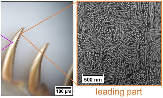
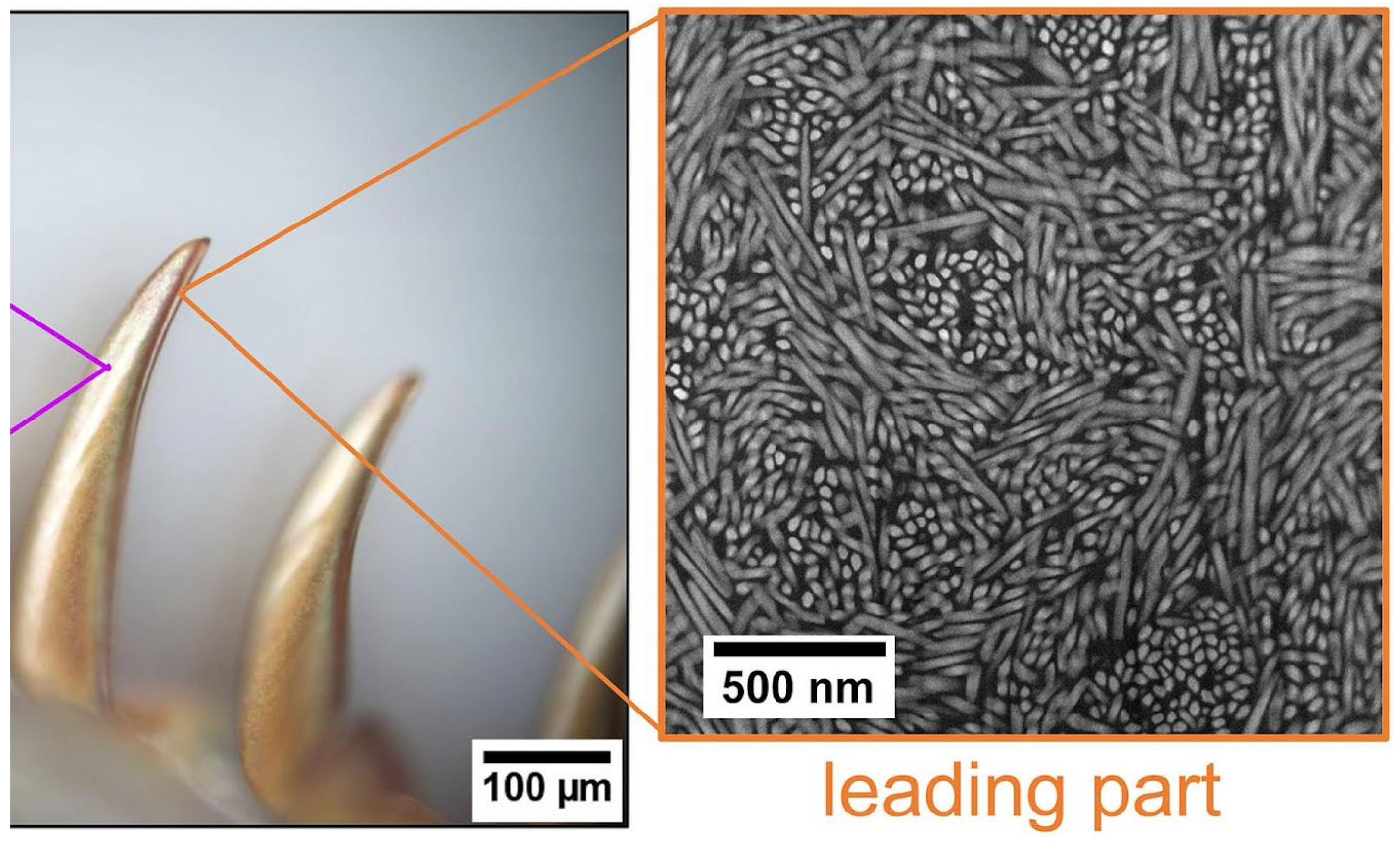
The exceptional mechanical properties of the limpet tooth can be attributed to its microstructure, which, in mature, fully mineralized limpet teeth, is functionally graded along the tooth’s longitudinal axis, ranging from a leading to a trailing region with distinct mechanical roles [24]. In the leading part, goethite nanorods (diameter 32 ± 0.4 nm, length 279 ± 18 nm, volume fraction of approximately 50% [24]) are organized into horizontally aligned nanorods weaving around vertically oriented nanorod bundles [24]: most nanorods run horizontally, while some vertically aligned bundles penetrate them (see Figure 1). The resulting three-dimensional pattern provides a high degree of interlocking and contributes to the exceptional strength and wear resistance of the leading part [23].
Figure 1.
Leading part of a limpet tooth: annular dark-field STEM microstructure (excerpt). Cropped from Figure 1 (leading part only; right-hand portion of the middle panel and the leading-part panel) in [22], licensed under CC BY 4.0 (https://creativecommons.org/licenses/by/4.0/). Changes: cropping.
At the nanoscale, the arrangement of goethite nanorods allows rotational motion of nanorods, enabling the composite to accommodate high mechanical loads through localized auxetic behavior [24]. This dual rotational mechanism enables localized stress redistribution within the composite and is considered the origin of the exceptional strength and stiffness of the leading tooth region [22,24]. The combination of auxeticity, high stiffness, and extreme strength is exceedingly rare among natural materials [24]. Consequently, the limpet tooth represents a unique example of natural materials engineering and provides valuable inspiration for the design of next-generation biomimetic and auxetic composite materials [22].
Remark: Auxeticity denotes a negative Poisson’s ratio (), meaning a material expands laterally when stretched [30,31]. Representative auxetic deformation mechanisms have been systematized by their underlying kinematics (e.g., rotation-, re-entrant-, chiral-, and instability-driven classes) [32]. Realizations span instability/buckling-induced systems (e.g., “Buckliballs” [33,34]), rotating rigid units [35], auxetic foams and related engineered cellular media [30,36], bistable concepts [37,38,39,40,41], tunable crystals and honeycomb-based composites [42,43,44,45], and carbon nanotube-network sheets [46,47]. Auxetic behavior is rare in biology but has been reported, e.g., in tendons [48], nacre [49], the osteodentin-based teeth of Atlantic wolffish [50], and limpet teeth [24]. Auxeticity in spider silks has been suggested but remains debated [51,52]. For cow teat skin, partially negative Poisson’s ratios have been reported; however, the evidence is incomplete and does not constitute confirmed auxeticity [53].
3. Dataset Generation
3.1. Geometric Idealization and Parameterization
To explore these complex structure–property relationships, a dataset of two-dimensional finite element simulations is generated [54]. Domain base is a square RVE of the leading region with a fixed edge length of 1 μm. All geometric parameters are expressed relative to this length scale.
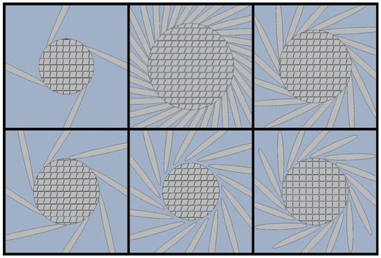
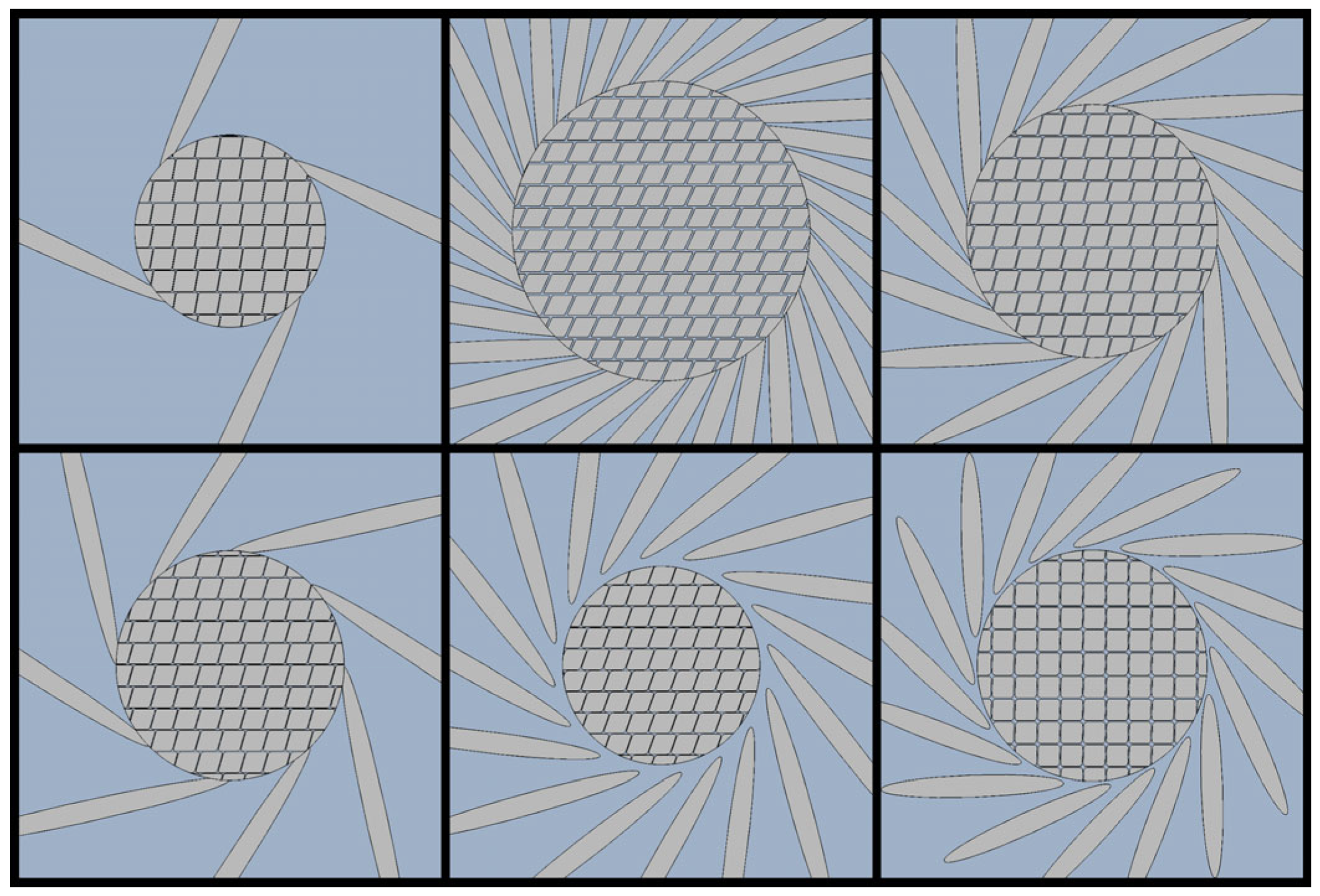
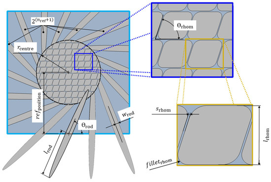
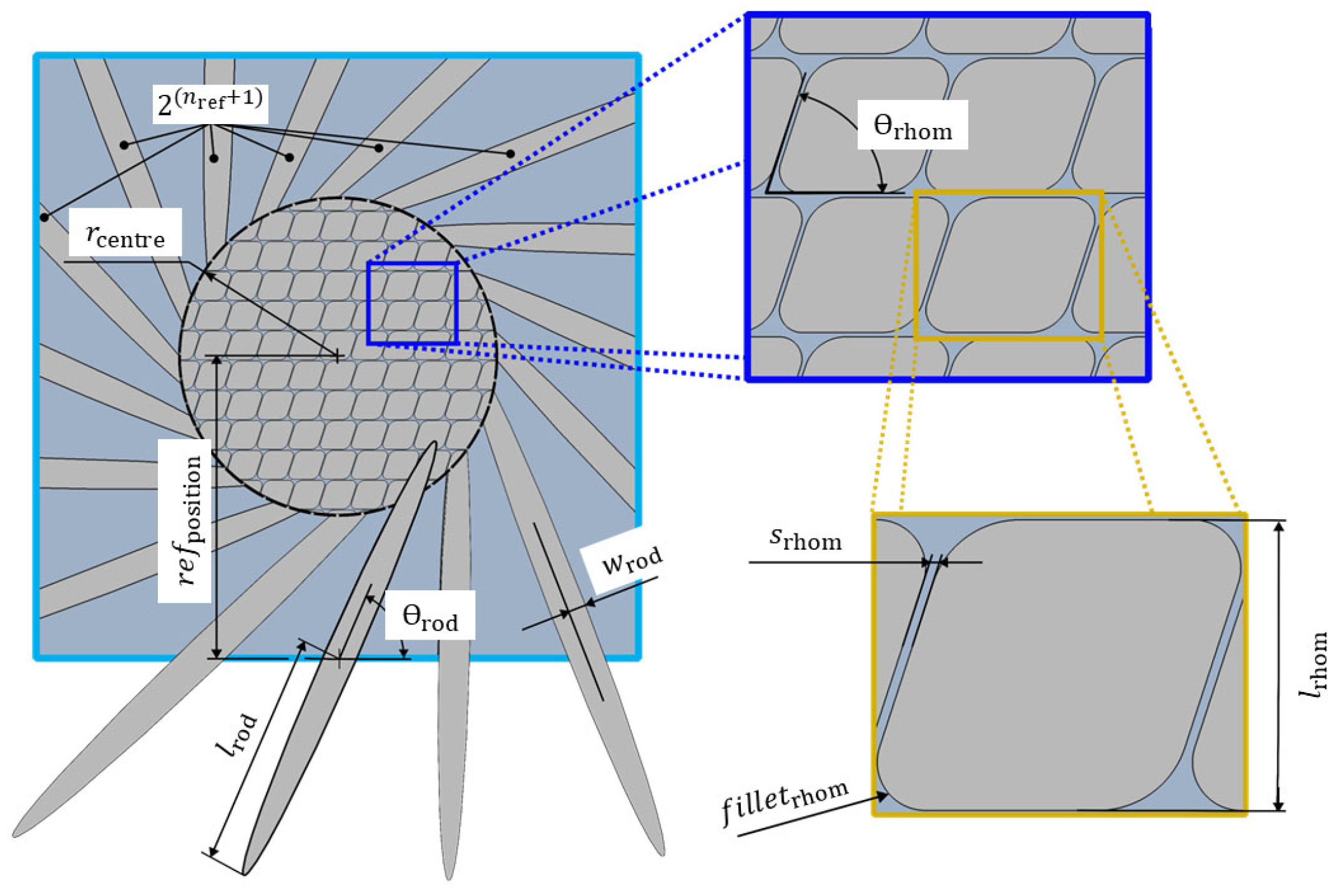
The outer nanorods are idealized as slender inclusions with elliptical cross-sections (arranged in a radially oriented pattern around the central cluster (Figure 2 and Figure 3)). Depending on the parameter choice, they either remain separated from the central region or locally intersect it. Their length, width and orientation are controlled by the half-length and half-width of the ellipses (i.e., the aspect ratio of the inclusions), while denotes the counter-clockwise angle that the lowest outer inclusion (lowest center in the vertical direction) makes with the horizontal axis, setting the global orientation of the outer inclusions. The total number of inclusions is given by .
Figure 2.
Examples of RVEs: They contain a central cluster of densely packed inclusions, surrounded by an outer inclusion region of radially arranged rods, embedded in a softer matrix phase.
Figure 3.
The cluster is idealized as a circular region of radius densely filled with congruent rhomboidal inclusions (i.e., the cross-sections of nanorods). The rhomboid edge length is the diameter of the inclusion, and is kept constant. The rhomboid angle controls whether the inclusion cross-section is closer to square or more rhombic. The inter-rhomboid spacing is as a fraction of the edge length, which leads to a high and essentially uniform packing density in the central cluster. specifies the filet radius relative to the rhomboid edge length. Increasing it transforms sharp-cornered rhombi into shapes that approach a circle.
In the actual material, the nanorods do not run parallel to one another; their axes are inclined at different angles to any given section plane and may also taper towards their ends [24]. A cut through the tooth intersects different rods at different positions, producing an apparently chaotic arrangement of cross-sections. The goethite nanorods are essentially defect-free and exhibit very similar maximum cross-sectional areas. Thus, nanorod cross-sections can be treated as identical in size, and moderate variations in their exact outline are.
3.2. Material Properties, Boundary Conditions and Loading
The finite element model treats the microstructure as a two-phase composite consisting of a stiff inclusion phase embedded in a softer matrix. Both phases are assumed to be linear-elastic and isotropic. We vary , and to explore a spectrum of stiffness contrasts and phase combinations while keeping the inclusion Young’s modulus fixed at a value representative of goethite (Table 1). We quantify phase elastic contrast via and explore how variations in matrix stiffness and constituent Poisson’s ratios influence the effective mechanical response in our two-phase inclusion–matrix model.
Table 1.
Material parameters of the two phases, data taken from [25] and [55].
Macroscopic strain states are applied as periodic boundary conditions via control nodes and multipoint constraints. The effective elasticity tensor is obtained by probing the response to (1) a normal strain , (2) a normal strain , and (3) a shear strain , providing effective elastic properties (Young’s modulus, Poisson’s ratio) as targets for subsequent data analysis.
3.3. Database
All simulation results are compiled into a tabular database with a total of 30,004 entries: each row corresponds to a single RVE and each column to a scalar descriptor (1. input parameters controlling the geometry and material contrast, 2. intermediate microstructural descriptors derived from the phase distribution and 3. output quantities summarizing the effective elastic properties. The input set comprises the geometric and material parameters from 1., augmented by the binary connectivity indicator. The indicator flags whether the outer inclusions form a continuous path connecting the central cluster across the periodic boundaries.
Category 2 is represented by the global inclusion volume fraction and regional inclusion fractions and , which are treated as regression targets.
Further, category 3 includes scalar descriptors of the homogenized directional responses and . For each orientation-dependent quantity , we store a compact set of summaries using the placeholder :
- min_{name}: , min_E ();
- max_{name}: , max_E ();
- mean_{name}: , mean_E ().
Details of the procedure are provided in the Supplementary Materials Section S1.
4. Data Processing
At this stage, the dataset exhibits strong class imbalance (768 auxetic RVEs, 2.6% of 30,004), with each RVE uniquely represented by 18 features that were introduced earlier. Prior to downstream use, the feature set is converted into a numerical representation by standardization, missing-value imputation and one-hot encoding (details in Supplementary Materials Section S2). To account for imbalance during classification, class weighting is applied. However, the required weight ratio (≈38.13) is too severe for trustworthy calibrated predictions, and the classifier outputs are therefore not interpreted probabilistically.
4.1. Dataset Refinement by Monte Carlo-Based Design-Space Exploration and Filtering with Binary Classification
We perform Monte Carlo-based design-space exploration by repeatedly drawing admissible parameter vectors at random within prescribed bounds and using the resulting candidates to sample the feasible response manifold. This approach is widely used when the design space is large and rare, but physically meaningful responses must be discovered through systematic random exploration. In the metamaterials context, closely related Monte Carlo design-space sampling is used to generate diverse training data and to identify rare, high-performing configurations [56].
A random forest classifier (trained with the above weighting) is used primarily to obtain feature-importance rankings. The corresponding ranking procedure and consolidation of encoded variables into raw design-variable groups are described in the Supplementary Materials. A direction label (high/low/none) is assigned to each raw design variable from the difference in the subgroup means (auxetic minus non-auxetic) and the sign of its correlation with the auxetic label. The resulting importances and directions are combined in a focused Monte Carlo scheme that draws influential variables from the empirically relevant upper or lower tails (Figure S4), while sampling all remaining variables uniformly to preserve broad coverage of the design domain.
This scheme is used to generate twice ca. candidate designs per Monte Carlo generation, with a large fraction of “focused” samples concentrated near auxetic-favorable directions. Each candidate remains within a physically plausible, FEM-proven design box, but sampling density is increased in regions where the learned importance structure indicates elevated auxetic potential.
Each candidate design is mapped through the fixed preprocessing pipeline (imputation, scaling and one-hot encoding of ) and evaluated by two binary surrogate classifiers (RF and FCNN), yielding predicted auxetic probabilities and . Here, denotes the design vector comprising the subset of direct geometric and material design variables (see Supplementary Materials Section S4). Candidates are ranked by
and only high-scoring designs () are retained (Figures S2 and S3), resulting in a reduced set of high-confidence auxetic proposals per Monte Carlo generation. High-scoring candidates are converted into FEM-ready inputs, simulated, and added to the dataset (5412 new entries). The final dataset comprises 35,416 RVEs, with an increased auxetic fraction from 2.6% to 15.5%.
4.2. Reduction in Non-Auxetic Data
To mitigate the persistent underrepresentation of auxetic RVEs even after the Monte Carlo-based enrichment, the non-auxetic subset is reduced. At this stage, the non-auxetic pool includes 29,929 non-auxetic RVEs: 29,236 original plus 693 newly generated. We apply K-means clustering to the non-auxetic RVEs in the standardized input-feature space (z-score normalization of all features listed in the Supplementary Materials). We use up to 3000 clusters (capped by the dataset size). Each non-auxetic RVE is assigned to exactly one cluster. Within each cluster, a cluster-size–proportional number of representatives is selected as the RVEs nearest to the cluster centroid in feature space. The remaining non-auxetic samples are discarded. Roughly 2–3 samples per cluster are kept on average, with more retained from larger clusters. This yields a substantially more balanced dataset of 13,717 entries in total (40% auxetic vs. 60% non-auxetic) without losing good coverage of the non-auxetic design space (Figure S5). The number of non-auxetic RVEs is reduced from 29,929 to 8230. The dataset is finally screened for consistency and cleaned accordingly.
5. Machine Learning Framework
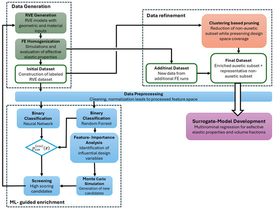
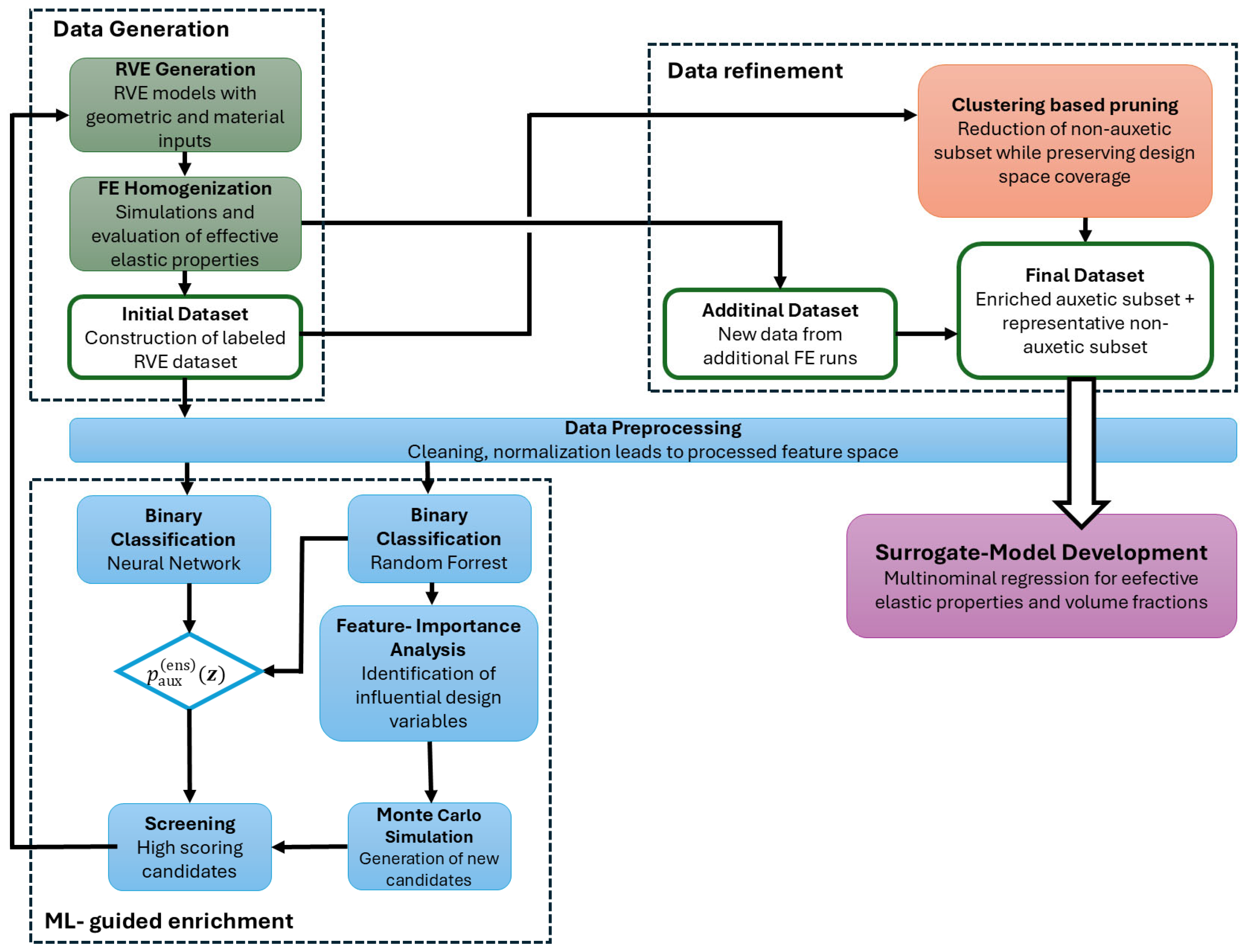
We use machine learning (Figure 4) with four complementary objectives, some of which are integrated into data processing. Implementation details (feature preprocessing, model architecture, training setup and clustering) are provided in Supplementary Materials.
Figure 4.
Schematic overview of the methodological workflow, from parametric RVE generation and FE homogenization to dataset construction, ML-guided dataset refinement, and surrogate-model development.
- Supervised models and feature-importance measures provide a descriptive view of which geometric and material parameters govern auxetic behavior in limpet-inspired microstructures.
- These insights are used to run additional simulations that enrich the dataset in regions where auxetic response is likely (cf. Section 4.1).
- The remaining class imbalance is addressed by pruning the non-auxetic subset via clustering-based prototype selection while keeping the design space well represented (cf. Section 4.2).
- Predictive surrogate models approximate FE homogenization and act as simulation-substitution models in the sense of deep-learning studies in computational mechanics [15], constituting the focus of this section.
We train supervised multi-output regression surrogates that map the processed 18-dimensional input vector (proc_*) of geometric and material parameters to effective elastic properties. Nine regression targets are drawn from the microstructural and effective properties: inclusion volume fractions (, , ) and directional summaries of and (, , , , , ; cf. Figure S1). Since the target components differ markedly in physical scale and numerical magnitude, each target is standardized to zero mean and unit variance prior to training, improving numerical conditioning and optimizer behavior for neural network surrogates. Targets and their descriptive statistics are reported in Table 2.
Table 2.
Targets for regression surrogates (13,717 samples).
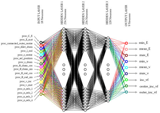
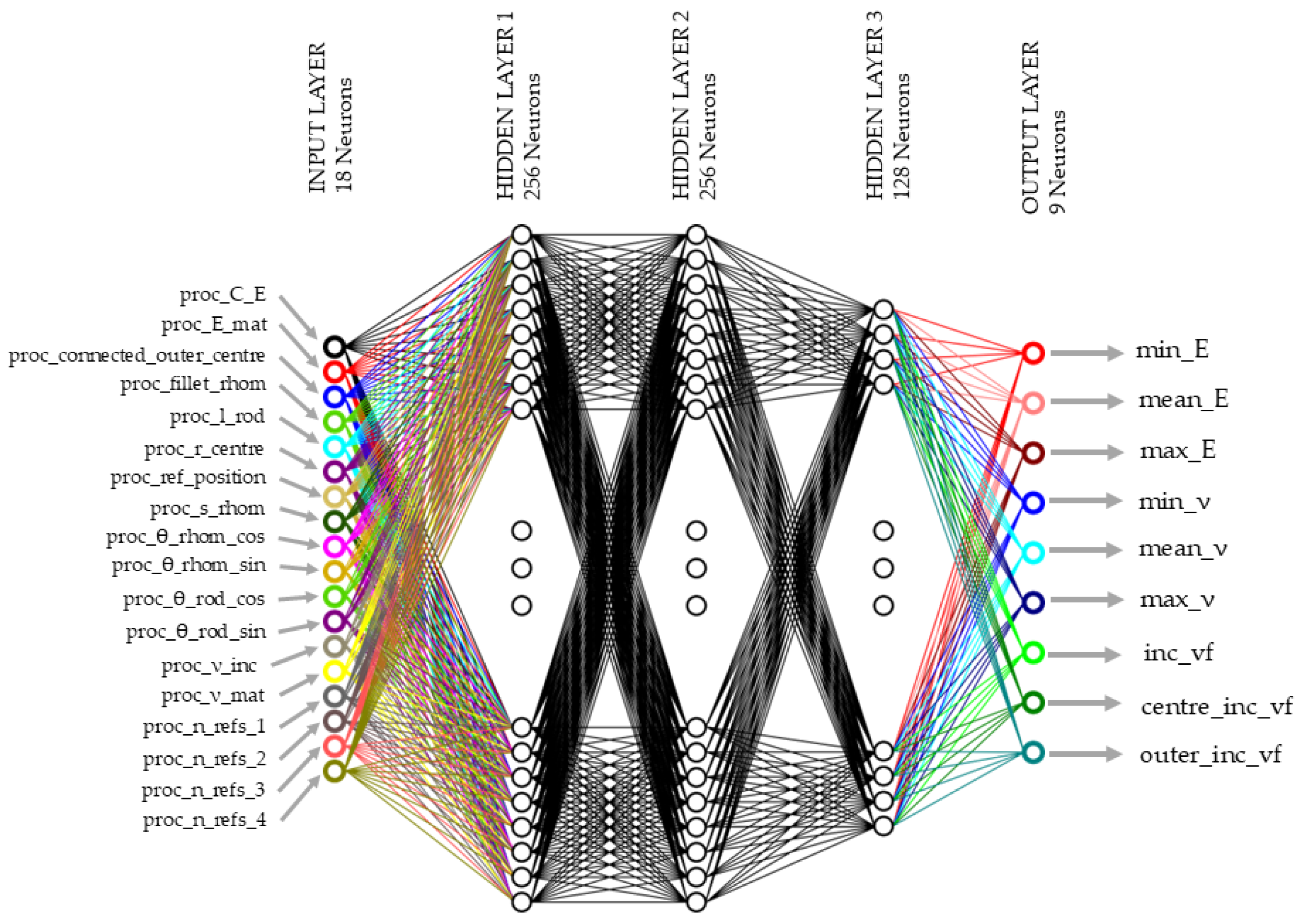
As an initial neural network surrogate, we start with a fully connected neural network (FCNN) with three hidden layers of widths (256–256–128; cf. Figure 5). This base configuration is used as the anchor architecture for the split-robustness checks and as the starting point for the subsequent validation-based sensitivity studies.
Figure 5.
Sketch of FCNN regressor (here: initial/base architecture). The network comprises three dense hidden layers with widths (256–256–128).
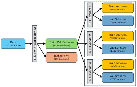
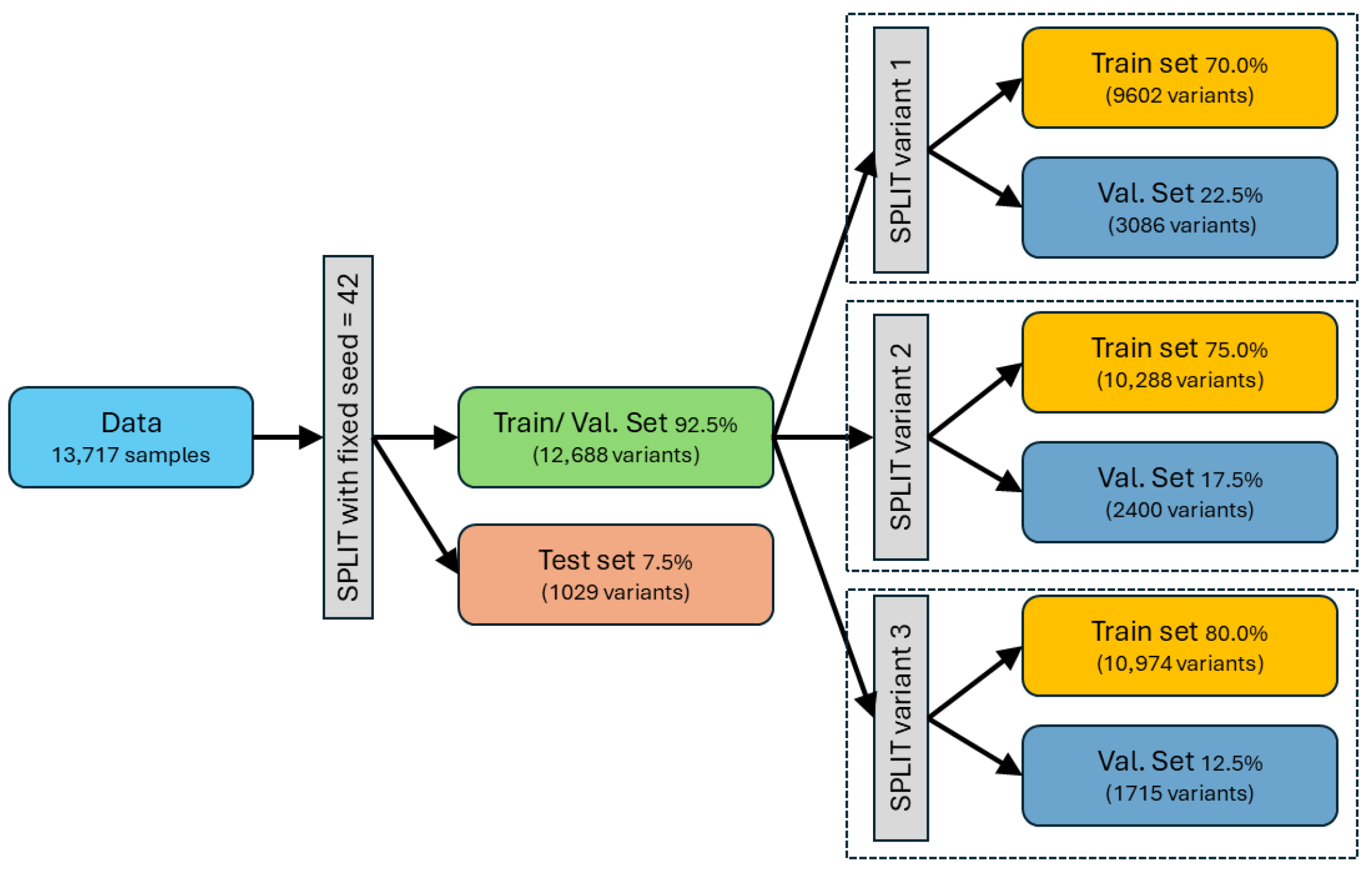
The dataset of 13,717 RVEs is first partitioned into a fixed stratified independent test subset and a remaining train/validation pool, with stratification based on the binary auxetic indicator to preserve the auxetic fraction across all subsets. Model development and model selection are carried out exclusively within the train/validation pool using validation-driven checkpointing and early stopping, whereas the test set is reserved solely for final external evaluation. To verify that the overall evaluation protocol is not tied to a particular partitioning choice, we additionally examine three alternative train/validation/test split ratios (cf. Figure 6), each combined with 11 train/validation split seeds, yielding 33 training runs in total. Based on this split-robustness analysis (cf. Supplementary Materials Section S7 and Figure S6), the 80.0%/12.5%/7.5% partition with train/validation seed 101 is retained for the subsequent studies.
Figure 6.
Data partitioning scheme used in the split-robustness study.
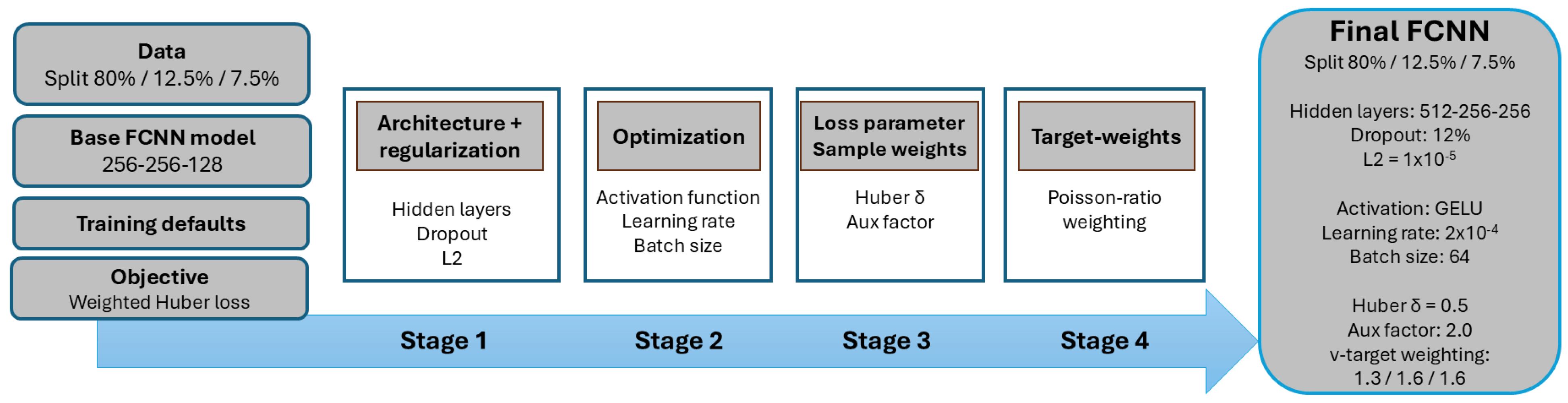
The FCNN hyperparameter sensitivity is then examined in four successive stages: architecture and regularization, optimization settings, loss parameters with sample weighting, and target-weight selection (details and results reported in Supplementary Material Section S8/Figures S7–S11). The final validation-based selection yields the FCNN configuration used in the main study, comprising three dense hidden layers with widths (512-256-256; cf. Figure 7).
Figure 7.
Schematic overview of the staged FCNN sensitivity and model-selection workflow.
Each hidden layer applies an affine transformation with L2 weight regularization, followed by layer normalization and dropout (12%) [57,58]. Nonlinearity is introduced via the activation function GELU, an alternative to ReLU that avoids a hard threshold at zero and can yield more stable gradients near the activation boundary [59,60]. The output layer is linear with nine neurons, yielding a prediction vector .
We minimize a weighted Huber-type loss which behaves like a squared error for small residuals and transitions to absolute-error-like growth for large residuals, thereby reducing sensitivity to occasional large deviations [61]. The loss is evaluated in the standardized target space and aggregated across the nine outputs using target-wise weights and a Huber transition threshold .
With class imbalance already substantially reduced by the enrichment procedure, auxetic samples receive only moderate additional weighting during regression training; the retained final configuration uses an upweighting factor of 2.0.
We use Adam as a standard optimizer for neural network regression due to its ease of tuning, with an initial learning rate of and gradient-norm clipping (clipnorm = 1.0) for update stability [62,63].
Training is run for up to 500 epochs but is regularized by validation-driven stopping and scheduling. Early stopping monitors the validation loss and terminates training if no improvement is observed for 20 consecutive epochs (patience = 20), at which point the weights from the best-performing epoch are restored. This prevents unnecessary over-training once generalization saturates. The learning rate is reduced by a factor of 0.5 when the validation loss fails to improve for eight epochs (ReduceLROnPlateau, patience = 8, min_lr = ), which refines the solution after the initial fast descent phase. Finally, model checkpointing retains the parameter set achieving the minimum validation loss, ensuring that the reported surrogate corresponds to the best validated model state. The network is implemented in TensorFlow/Keras [64], and the code is provided in Supplementary Materials Section S6. Its performance is benchmarked against representative tree- and kernel-based nonlinear baselines (RF and SVR):
- Tree-based baseline: A random forest regressor with 400 trees is trained as a multi-output regressor using the same processed input representation. Sample-wise weights are applied during fitting to emphasize auxetic realizations.
- Kernel-based baseline: As a classical nonlinear surrogate, an RBF-kernel support vector regression is trained using a MultiOutputRegressor wrapper with a single shared hyperparameter setting (, ).
All regression models are evaluated on the validation subset using per-target and aggregated metrics.
Remarks:
- Activation function: The Rectified Linear Unit passes positive inputs unchanged while setting negative inputs to 0 [59]. The Gaussian Error Linear Unit gates the input by the probability that a standard normal variable is below , where is the standard normal cumulative distribution function. GELU is often implemented via the smooth approximation [60]. Compared to the hard zero-thresholding of ReLU, GELU provides a smooth, probabilistic gating near , which can improve gradient behavior around the activation boundary.
- Weighted Huber loss: For each target component , the residual is computed in standardized space. The Huber penalty is quadratic for and linear for , limiting the influence of large residuals [61]. corresponds to an absolute residual of one standard deviation for the respective standardized target component. Target-wise weights scale the contribution of each output in the aggregated loss, target order (, , , , , , , , ). During training, auxetic samples additionally receive a sample-wise weighting factor,
- Adam adapts per-parameter step sizes using bias-corrected moving averages of the gradient (first moment) and squared gradient (second raw moment), stabilizing mini-batch training [62].
- Clipnorm (gradient-norm clipping) caps the global -norm of the gradient to avoid sporadically large updates [63].
6. Results and Discussion
The original database comprises 30,004 simulations, in which auxetic responses are rare (2.6%). To enable statistically meaningful analysis of the auxetic regime and to support subsequent surrogate modeling, the database is consolidated into a rebalanced dataset containing 13,717 simulations with an auxetic fraction of ca. 40% (5487 entities).
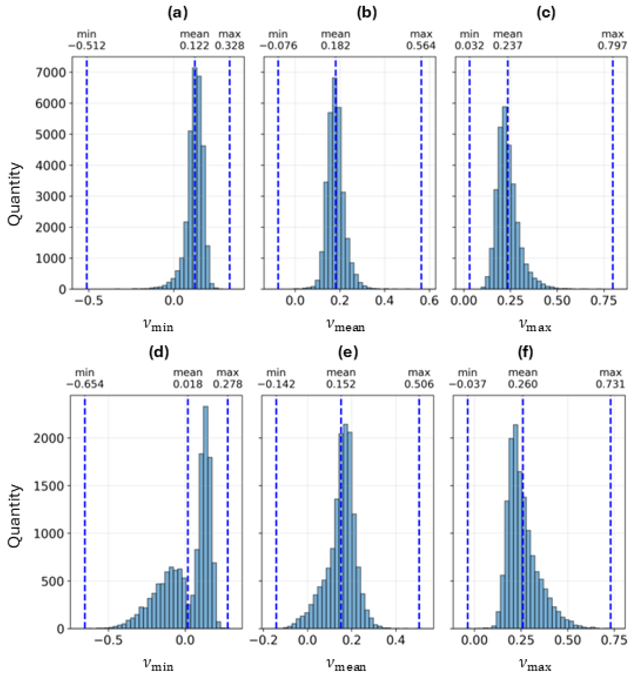
In the original dataset, all three scalar summaries of the directional Poisson response are centered in the positive regime, consistent with the low incidence of auxetic behavior (Figure 8). For , the distribution is concentrated around a positive mean (0.122) with an interquartile range (IQR) of 0.100–0.155, while negative values occur only in the extreme left tail (minimum −0.512). The same pattern is even more pronounced for : the central 50% of realizations lies between 0.157 and 0.202 (mean 0.182), and the most negative observed value is only −0.076. Finally, remains strictly positive across the entire dataset (minimum 0.032), with the bulk of samples between 0.197 and 0.265 (mean 0.237). Thus, auxeticity is not a dominant global response mode in the original database. Rather, it appears primarily as a limited negative excursion in the orientation-dependent response, captured most sensitively by , while remains positive.
Figure 8.
Ground-truth effective Poisson’s ratio (computed from FEM) using three statistics: , and . These descriptors are derived from the direction-dependent response . (a–c) Database before enrichment; (d–f) “Enriched” and “prunged” database.
After enrichment and pruning, the negative- regime is substantially better represented, and the distribution broadens and shifts downward. Its IQR now crosses into the auxetic regime (−0.092–0.138) with a mean of 0.018, compared with the strictly positive IQR in the original dataset (0.100–0.155, mean 0.122). While remains centered in the positive regime (IQR 0.122–0.193, mean 0.152), its negative range expands (min. −0.142 vs. −0.076 originally), indicating increased representation of RVEs with auxetic response over certain orientations. The distribution remains predominantly positive in both datasets, with comparable central tendency (IQR 0.201–0.301, mean 0.26 vs. IQR 0.197–0.265, mean 0.237) and only moderate changes in the upper range (max. 0.731 vs. 0.797).
The dataset curation increases sample density and resolution in the auxetic tail—reflected by —while preserving the broader non-auxetic response manifold. The stronger shift in relative to suggests that many auxetic responses manifest as localized or state-dependent behavior, while the average response may remain near or above zero.
Rebalancing redistributes sampling density without collapsing the variability of the design space: There is a moderate shift toward lower stiffness ([GPa]: 11.48/12.39/13.42 8.42/9.34/10.45), while maintaining a broad feasible range (max. [GPa]: 68.06 vs. 61.47). Volume-fraction statistics change only moderately (: 33.3% 34.5%; : 76.7% 81.8%; : 19.4% 19.9%), see Figures S12 and S13. As a consequence of data resampling, the negative- regime is no longer statistically marginal. This mitigates the imbalance-induced bias of standard regressors toward the dominant non-auxetic regime and improves their ability to learn the transition between non-auxetic and auxetic behavior. At the same time, the final dataset remains physically diverse.
We next present quantitative surrogate-model performance on the consolidated dataset by comparing a fully connected neural network regressor against two standard baselines—SVR and RF—across the full multi-output target set. The reported physical validation and test metrics are unweighted, but they are indirectly affected by auxetic sample weighting because model optimization and validation-based model selection are performed using weighted samples.
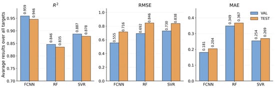
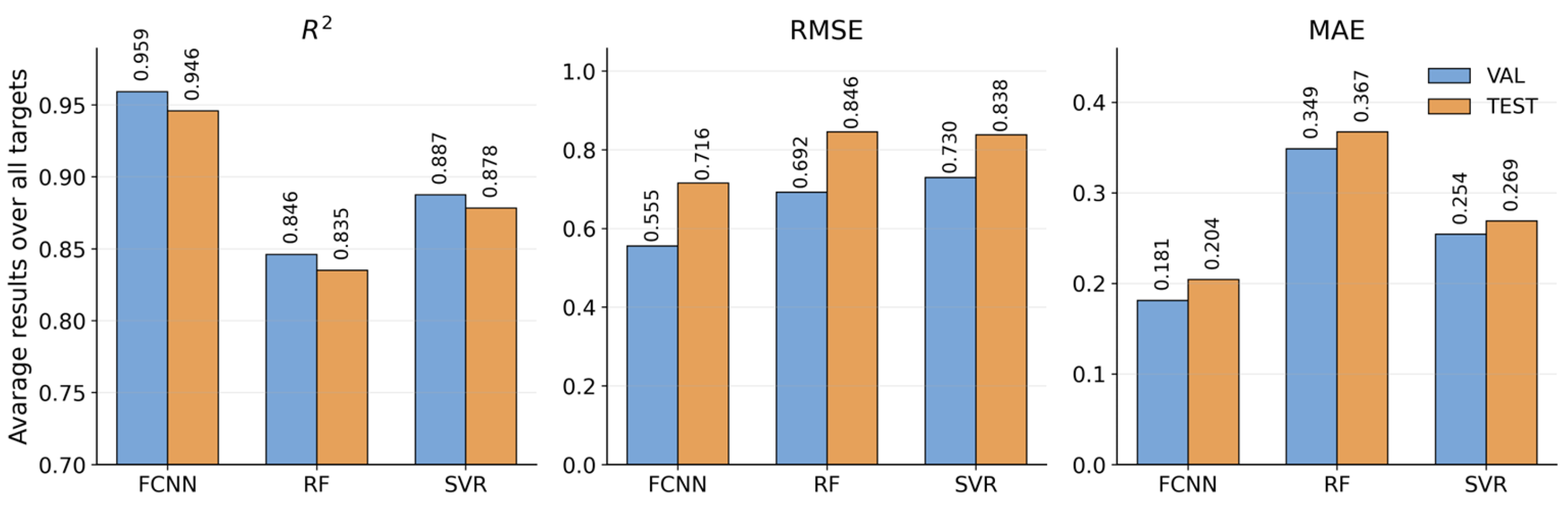
Across both splits, the FCNN remains the best-performing surrogate, achieving the highest mean and the lowest and . On the validation set, the FCNN reaches , , and ; on the independent test set , , and (cf. Figure 9). The model ranking remains unchanged from validation to test, with SVR consistently ranking second overall and RF third. This stable ordering, together with the moderate performance decrease from validation to test, indicates good generalization of the FCNN and no evidence of a model reversal on unseen data.
Figure 9.
Average regression performance over all nine outputs for the validation (VAL) and independent test (TEST) sets, reported as averaged , RMSE, and MAE over the nine target variables.
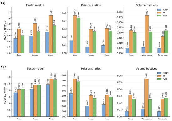
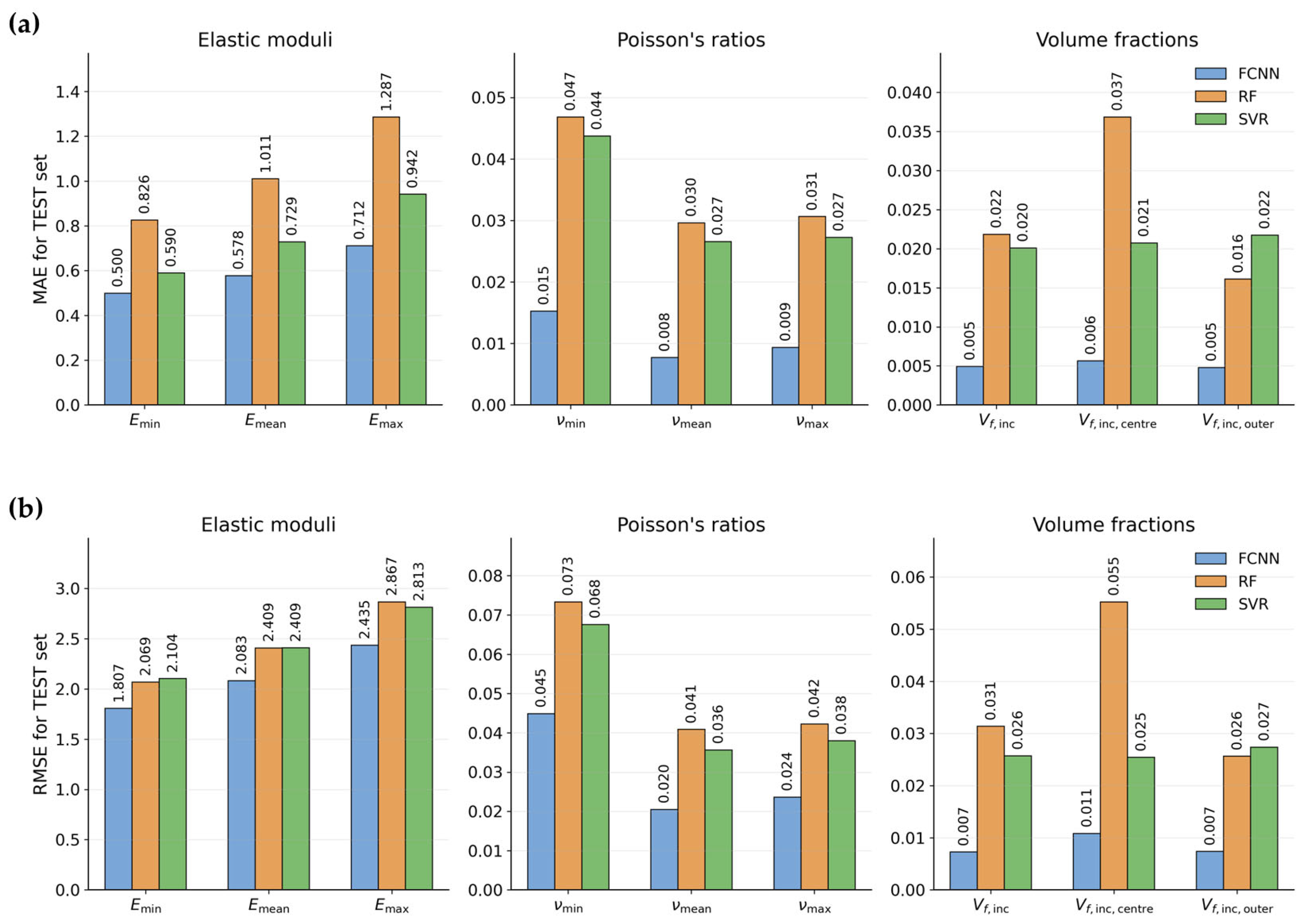
Since absolute error magnitudes are not directly comparable across all physical quantities, Figure 10 resolves the test-set errors by target family, separating elastic moduli, Poisson’s ratios, and volume fractions. The FCNN yields the lowest MAE and RMSE for all nine targets, showing that its advantage is not limited to the average metrics in Figure 9. This pattern is consistent at the per-target level across both validation and test sets (cf. heatmaps in Figures S14–S16).
Figure 10.
Per-target regression errors on the independent test set for FCNN, RF, and SVR, grouped by output family: (a) MAE and (b) RMSE for elastic moduli, Poisson-ratio descriptors, and volume fractions.
In terms of Poisson’s ratios, the FCNN maintains a pronounced margin in both absolute error and , whereas RF and SVR deteriorate more strongly, especially for , which gives the lowest test set among these descriptors for both baselines, and for , which carries the largest absolute errors overall. This indicates that capturing the auxetic-response-related part of the surrogate task is substantially more demanding than predicting the stiffness-related or geometric-fraction outputs. In this target family, SVR remains consistently closer to the FCNN than RF but still shows a clear loss in fidelity relative to the neural network surrogate.
For the elastic moduli, all three models perform more robustly, but FCNN again gives the smallest errors across , , and . The gap between SVR and RF is smaller than for the Poisson-ratio targets, yet the SVR is generally the stronger baseline, particularly for and , where its MAE and RMSE remain noticeably below those of RF. This suggests that the modulus-related trends are comparatively easier to learn, although the FCNN still provides the most accurate and most balanced approximation across the full range of stiffness descriptors.
The volume-fraction outputs are predicted very accurately overall, which is reflected by the near-unity values (Figure S14). However, this target family also reveals a specific weakness of RF: the center inclusion volume fraction is associated with a markedly larger error than for the FCNN and substantially worse than for SVR. By contrast, RF is more competitive for , where its errors are close to, and in MAE slightly below those of SVR. Thus, the main performance penalty of RF is not a uniform degradation over all volume-fraction targets, but rather a pronounced difficulty in resolving the partitioning of inclusion content into the central region.
Overall, the per-target analysis shows that the main strengths of the FCNN are its uniformly low error levels, its stable ranking from validation to test, and its particularly strong handling of Poisson’s ratios, which are the most demanding outputs in the surrogate task. The main weaknesses of the classical baselines are therefore target-specific rather than global: for SVR, the largest deficits remain concentrated in the Poisson-ratio family, while for RF the most severe deficits occur for Poisson-ratio prediction and for the center inclusion volume fraction. Accordingly, the largest potential for future improvement lies in better resolving auxetic-response-sensitive descriptors.
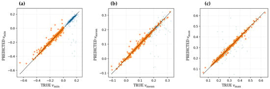
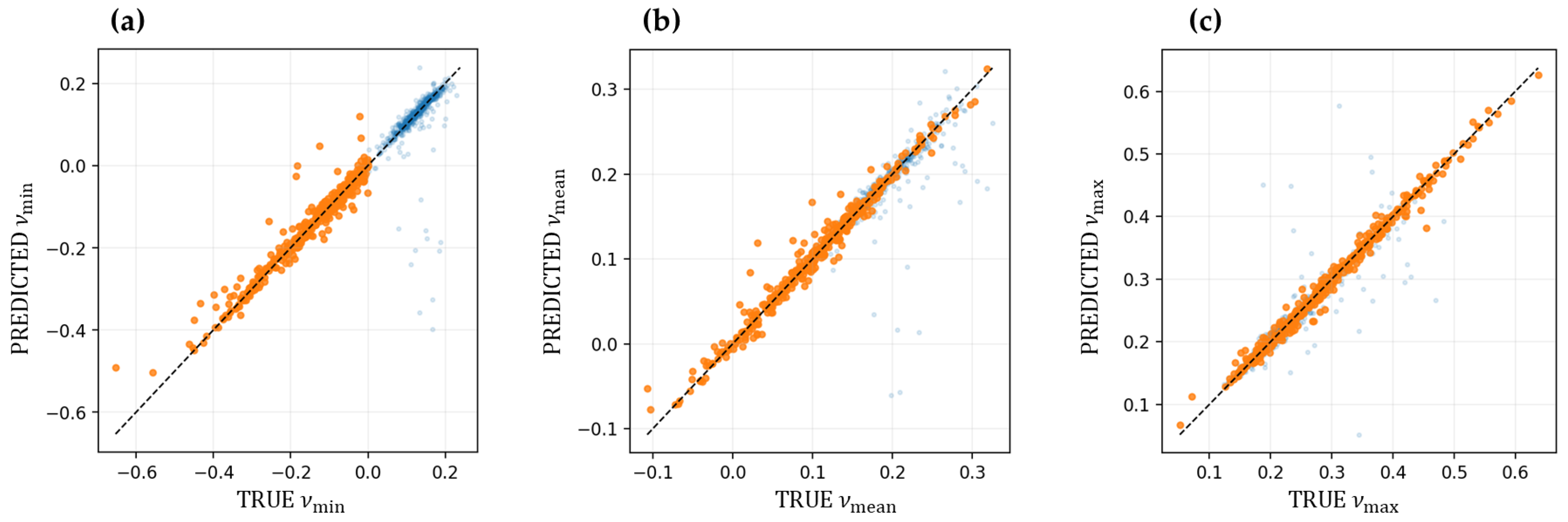
We further examine predictive fidelity for the Poisson-related targets using parity plots for , and (Figure 11a–c). Predicted and FE-derived values cluster closely around the identity line, confirming good calibration and good generalization to unseen data. The agreement remains particularly tight for and over most of the observed range, consistent with the strong per-target results in Figure 10 and Figures S14–S16.
Figure 11.
Observed vs. predicted Poisson’s ratios on the hold-out validation subset (FCNN): (a) , (b) , and (c) . Orange markers denote data points for which the FE simulations yielded < 0, whereas the blue markers correspond to non-auxetic cases. On the left, a clear vertical separation is visible at = 0.0.
The parity plot for (Figure 11a) is the most demanding since defines the onset of auxetic response. Here, the model reproduces the transition region near with high fidelity and maintains good agreement in the auxetic regime. At the same time, the largest pointwise deviations are concentrated in the most negative and most positive extremes of , where lower sample density makes tail behavior more difficult to learn. This behavior is expected for tail-dominated targets and emphasizes the utility of reporting , and jointly; while probes the onset of auxetic mechanisms through directional excursions, and reflect the broader non-auxetic response manifold.
FCNN not only achieves strong aggregate accuracy but also preserves physically relevant distinctions between the auxetic tail and the broader non-auxetic response manifold (Figure 11; see also the corresponding validation-set parity plots in Figure S17 and the parity plots for the elastic-modulus and volume-fraction descriptors in Figures S18–S21).
To contextualize surrogate performance beyond aggregate test metrics, we analyze two representative cases: a leading-part regime anchored to experimentally reported limpet-tooth properties and a curated set of exemplars spanning clearly auxetic, near the auxetic–non-auxetic transition, clearly non-auxetic, and distributionally atypical (‘hard’) designs identified as outliers in the input-feature space to provide an interpretable overview of model behavior.
6.1. Case 1: Leading-Part Regime
The leading part of limpet teeth exhibits an elastic modulus of 38.4 ± 6.2 GPa, Poisson’s ratios centered near zero (≈−0.01 ± 0.09), and an inclusion volume fraction of ~50% (experimentally 51.5 ± 1.8%) [24]. We therefore choose a small set of RVEs whose inclusion volume fraction () is close to 50% and whose effective Poisson response includes near-zero and slightly negative regimes (see Table 3).
Table 3.
Summary statistics (min/mean/max) for selected RVEs (), leading-part regime.
All errors below are absolute errors evaluated per target over the RVEs. Aggregated predictive errors are summarized in Table 4. Overall, the surrogate retains high fidelity in this regime, with particularly small deviations for the Poisson ratios and volume fractions. For , the mean absolute errors remain on the order of –, while the corresponding maxima stay below . The largest deviation occurs for in a near-boundary case (, ), confirming that the most sensitive behavior is concentrated close to the auxetic decision threshold. This supports the use of absolute rather than relative errors for Poisson-related quantities, especially in the vicinity of .
Table 4.
Aggregated results of comparison of predictions vs. ground truth from FE simulations.
For the effective Young’s moduli, the errors are likewise moderate: the mean absolute error increases from about GPa for to GPa for , and the maximum absolute errors remain limited to about – GPa. Notably, the same RVE produces the maxima for all three moduli, indicating a localized hard case within this otherwise well-predicted subset. The volume-fraction targets are also reproduced accurately, with mean absolute deviations of about –% and a worst-case deviation of about % for . These trends are consistent with the tight clustering around the parity line in Figure 12 and Figures S22 and S23; the per-RVE ground-truth and predicted values with absolute errors are listed in Tables S2–S4.
Figure 12.
Case “leading part”: Parity plots for Poisson’s ratios on selected RVEs (predicted based on trained FCNN regressor model): (a) , (b) and (c) . Orange markers: auxetic samples, blue dots: non-auxetic samples.
While these RVEs match the intended ~50% inclusion volume fraction criterion well, their effective elastic moduli (~ 18–27 GPa) are lower than the experimentally measured modulus (38.4 ± 6.2 GPa). Thus, the present selection represents a qualitative, regime-consistent benchmark (matching volume fraction and near-zero Poisson’s response), but not a direct one-to-one reproduction of the experimental data.
6.2. Case Study 2: Curated Exemplars Spanning Response Regimes
We next evaluate surrogate behavior on a curated set of exemplars that spans qualitatively different Poisson-response regimes: (a) clearly auxetic behavior, (b) near-boundary cases close to the auxetic/non-auxetic transition, (c) clearly non-auxetic behavior and (d) hard cases identified by the largest robust outlier score. Here, the outlier score serves as a practical proxy for “out-of-distribution” behavior: large values indicate that a candidate deviates simultaneously across multiple physically interpretable features relative to the reference distribution.
The resulting set covers a wide range of effective properties (Table 5), including negative down to approximately and positive up to . The inclusion volume fraction spans distinct regimes () and the effective Young’s modulus varies from very compliant to moderately stiff responses ( GPa), thereby intentionally probing the surrogate outside the leading-part regime.
Table 5.
Summary statistics (min/mean/max) for selected RVEs (n = 8) from a new simulation set.
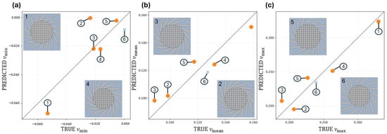
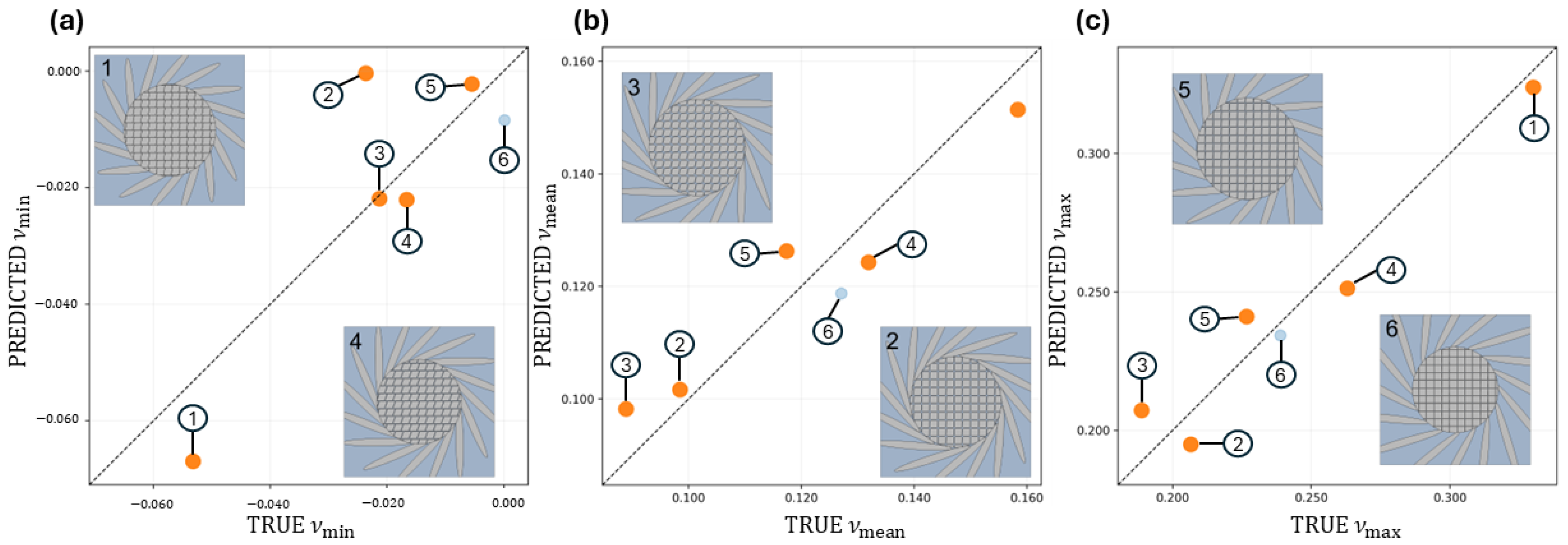
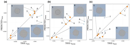
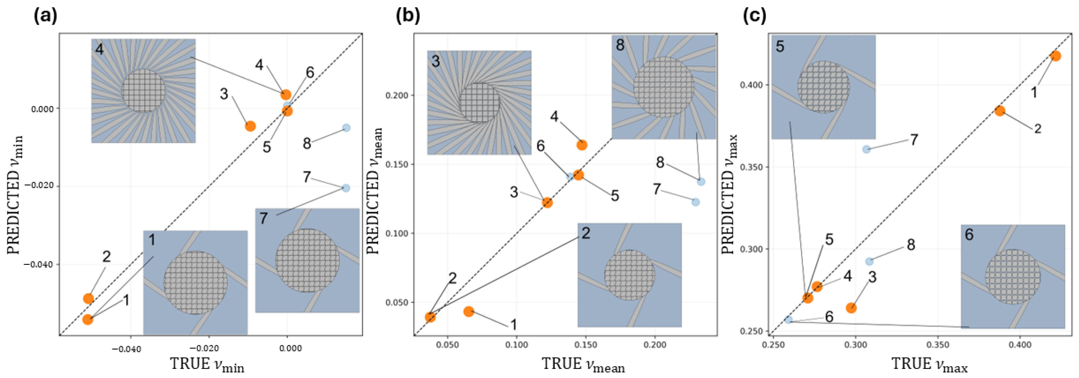
Overall, the surrogate reproduces the curated exemplars well, and its performance remains strong even in the immediate vicinity of the auxetic/non-auxetic transition. The near-boundary case RVE 4 () is predicted with only a small absolute deviation, although the sign changes because the prediction shifts to a small positive value. The neighboring near-zero non-auxetic cases, RVEs 5 and 6, are reproduced almost exactly (Figure 13). Thus, the boundary region itself does not appear to be a systematic weakness when assessed in terms of absolute error.
Figure 13.
Parity plots for the Poisson’s ratios on selected RVE representations (predicted based on trained FCNN regressor model): (a) , (b) and (c) . Orange markers: auxetic samples, blue dots: non-auxetic samples.
The dominant discrepancies are instead concentrated in the hard, outlier-selected exemplars, namely RVEs 7 and 8. For these two cases, the largest -related errors occur in positive- samples for which the surrogate underpredicts strongly enough to cross into the negative range, and the largest deviations in are observed for the same RVEs (Table 6). A similar concentration is seen for the effective Young’s moduli, where the maxima of the absolute errors are again driven by RVEs 7 and 8. By contrast, the inclusion-volume-fraction targets remain comparatively stable across the set, especially and , while shows a noticeable increase only for these hardest cases (cf. Tables S5–S7 and Figures S24 and S25).
Table 6.
Aggregated results of comparison of predictions vs. ground truth from FE simulations.
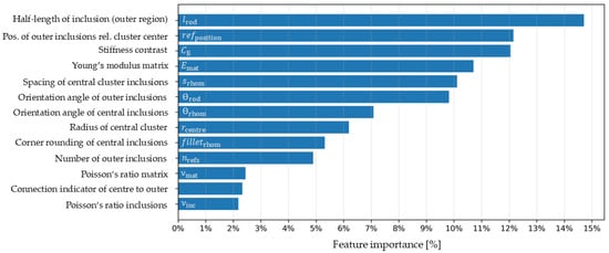
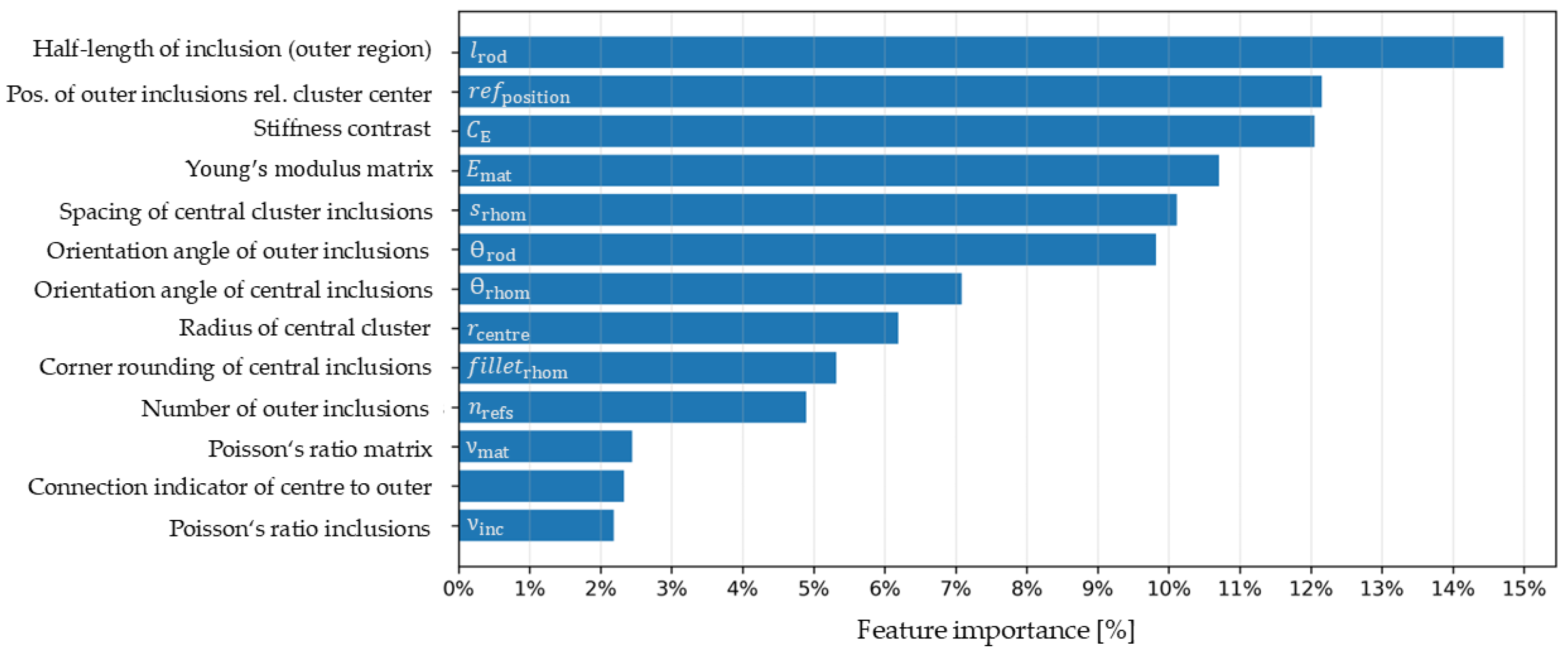
These results support the use of the surrogate for routine screening across qualitatively different response regimes. The observed error increase is limited mainly to the high-outlier-score exemplars RVEs 7 and 8, suggesting that any further refinement would be most valuable for such hard cases rather than for the whole dataset. This behavior is consistent with the targeted data-management strategy adopted for the strongly imbalanced design space. A key enabler is the extraction of a physically interpretable importance structure from the binary classification. A weighted random forest classifier is used to rank the contributions of the 18 raw design variables to auxetic behavior (Figure 14). For interpretability, these 18 columns are reported as 13 consolidated feature groups: is represented via one-hot encoding and the angular variables and are encoded by their sine/cosine components (, ), which are grouped as single underlying angle features. The resulting ranking is strongly concentrated and provides a clear physical narrative (Figure 12). The dominant contributions come from (14.7%) and (12.2%), which together account for 26.9% of the total importance. Including stiffness contrast (12.1%) and the Young’s modulus of the matrix (10.7%) brings the top four to 49.6%, and the top six features reach 69.6% once (10.0%) and (9.8%) are added—indicating that auxetic/non-auxetic separation is governed by a small set of dominant drivers rather than diffuse, weakly informative inputs.
Figure 14.
Feature-importance ranking of the raw design variables for auxetic behavior (random forest classifier).
Geometric descriptors dominate the separation. Aggregated across outer-geometry and cluster-geometry variables, they contribute 72.6% of the total importance. Outer-region geometry alone (, , , , center–outer connection indicator) accounts for 43.9%. Central cluster descriptors (spacing , cluster radius , corner rounding and ) contribute a further 28.7%, indicating a secondary, but still substantial role of cluster packing and shape. The orientation variables and jointly contribute 16.9%, highlighting orientation as an important geometric control lever.
Material parameters contribute 27.4% and are largely concentrated in the stiffness contrast . Thus, auxetic behavior is driven primarily by geometry (especially outer-inclusion size/placement and cluster organization) and modulated by stiffness contrast, whereas Poisson’s ratio plays a minor role ( (2.4%) and (2.2%)).
These insights are then used to drive a targeted rebalancing of the dataset with minimal procedural overhead. Feature-importance-guided Monte Carlo screening (with candidates scored by an ensemble auxetic probability; see Equation (1)) yields 6105 high-confidence proposals across two generations. Subsequent FEM verification confirms 5412 of these as auxetic, substantially enriching the minority class. In parallel, redundancy in the non-auxetic majority is reduced via k-means-based representative downsampling, which compresses the dataset while preserving essential variability in the design space. Together, these two steps produce a markedly improved class balance and consequently, higher predictive fidelity of the regression-surrogate—an effect that is illustrated in the preceding case studies across distinct response regimes.
7. Conclusions
This work investigates data-driven surrogate modeling of the mechanical response in a limpet-tooth-inspired composite microstructure design space, with particular emphasis on reliably identifying and predicting auxetic regimes. Starting from a dataset with a pronounced class imbalance, we use RF/FCNN classification and RF-derived feature importances to guide targeted auxetic enrichment, followed by k-means-based representative downsampling of the non-auxetic majority to obtain a substantially more balanced training set. Training an FCNN regressor on this rebalanced dataset yields high predictive fidelity for the mechanical targets and consistently surpasses RF and SVR baselines, demonstrating that feature-guided rebalancing materially improves surrogate accuracy and screening efficiency.
Across the considered validation scenarios, the FCNN regressor remains accurate and preserves the expected qualitative trends, supporting robust use beyond the most frequently sampled regions of the design space. This enables rapid, low-overhead parametric studies and pre-screening without repeatedly constructing geometries, running FEM simulations and post-processing results, thereby substantially accelerating microstructure exploration. Future research may extend this framework to three-dimensional microstructures and application-oriented validation studies.
Supplementary Materials
The following supporting information can be downloaded at: https://www.mdpi.com/article/10.3390/mca31030077/s1, Figure S1: Example RVE; Figure S2: Design domain after Monte Carlo sampling; Figure S3: Potential designs after Monte Carlo sampling from the perspective of specific feature combination; Figure S4: Effect of focused Monte Carlo sampling on design-variable distributions; Figure S5: PCA projection of the non-auxetic design space with selected K-means representatives; Figure S6: Split-ratio robustness analysis for the retained reference FCNN; Figure S7: Architecture-and-regularization study; Figure S8: Heatmap summary of the architecture-and-regularization study (Stage 1); Figure S9: Heatmap summary of the optimization study for the shortlisted FCNN architectures (Stage 2); Figure S10: Heatmap summary of the loss-parameter and sample-weighting study (Stage 3); Figure S11: Heatmap summary of ν-target weighting sensitivity study (Stage 4); Figure S12: Global distribution of effective E Modulus over all simulations; Figure S13: Global distribution of volume fractions over all simulations; Figure S14: Per-target coefficients of determination (R2) for FCNN, RF, and SVR on the validation (VAL) and independent test (TEST) sets. Results are shown for all nine outputs, covering elastic moduli, Poisson-ratio descriptors, and volume fractions; Figure S15: Per-target mean absolute errors (MAE) for FCNN, RF, and SVR on the validation (VAL) (a-c) and independent test (TEST) sets (d-f), shown separately for elastic moduli (a,d), Poisson’s ratios (b,e), and volume fractions (c,f); Figure S16: Per-target root mean square errors (RMSE) for FCNN, RF, and SVR on the validation (VAL) (a-c) and independent test (TEST) sets (d-f), shown separately for elastic moduli (a,d), Poisson’s ratios (b,e), and volume fractions (c,f); Figure S17: Observed vs. predicted Poisson’s ratios on the validation subset; Figure S18: Observed vs. predicted elastic moduli on the validation subset; Figure S19. Observed vs. predicted elastic moduli on the hold-out test subset; Figure S20: Observed vs. predicted volume fractions on the validation subset; Figure S21: Observed vs. predicted volume fractions on the hold-out test subset; Figure S22: Case “leading part”: Parity plots for Elastic moduli on selected RVEs; Figure S23: Case “leading part”: Parity plots for the volume fractions on selected RVEs (predicted based on trained FCNN regressor model); Figure S24: Case Study 2: Parity plots for Elastic moduli on selected RVEs (predicted based on trained FCNN regressor model); Figure S25: Case Study 2: Parity plots for the volume fractions on selected RVEs (predicted based on trained FCNN regressor model); Table S1. Summary statistics for the original (unstandardized) feature values; Table S2: Poisson’s ratios (ground truth vs. prediction) with absolute errors for the six leading-regime RVEs (Case Study 1); Table S3: Elastic moduli (ground truth vs. prediction) with absolute errors for the six leading-regime RVEs (Case Study 1); Table S4: Volume fractions (ground truth vs. prediction) with absolute errors for the six leading-regime RVEs (Case Study 1); Table S5: Poisson’s ratios (ground truth vs. prediction) with absolute errors for the eight RVEs (Case Study 2); Table S6: Elastic moduli (ground truth vs. prediction) with absolute errors for the eight RVEs (Case Study 2); Table S7: Volume fractions (ground truth vs. prediction) with absolute errors for the eight RVEs (Case Study 2).
Author Contributions
Conceptualization, S.B. and A.H.; methodology, S.B. and A.H.; software, A.H. and B.A.; validation, A.H.; formal analysis, A.H.; resources, S.B.; data curation, A.H. and B.A.; writing—original draft preparation, A.H.; writing—review and editing, S.B. and B.A.; visualization, A.H.; supervision, S.B.; project administration, S.B.; funding acquisition, S.B. All authors have read and agreed to the published version of the manuscript.
Funding
This research was funded by Deutsche Forschungsgemeinschaft (DFG, German Research Foundation), grant number 529221905.
Data Availability Statement
The original contributions presented in this study are included in the Supplementary Materials.
Acknowledgments
During the preparation of this manuscript, the authors used ChatGPT (OpenAI, GPT-5.2) for improving grammar and language clarity and assisting with drafting Matplotlib code for graphical post-processing and visualization of results. The authors have reviewed and edited the output and take full responsibility for the content of this publication.
Conflicts of Interest
The authors declare no conflicts of interest.
Abbreviations
2D: two-dimensional, Adam: adaptive moment estimation optimizer, FCNN: fully connected neural network, FE: finite element, FEM: finite element method, GELU: Gaussian Error Linear Unit, IQR: interquartile range, MAE: mean absolute error, RBF: radial basis function, ReLU: Rectified Linear Unit, RF: random forest, RMSE: root-mean-squared error, RVE: representative volume element, SVR: support vector regression
References
- Alheit, B.; Bargmann, S.; Reddy, B.D. How suture networks improve the protective function of natural structures: A multiscale investigation. Acta Biomater. 2022, 145, 283–296. [Google Scholar] [CrossRef] [Scilit]
- Liu, Z.; Bessa, M.A.; Liu, W.K. Self-consistent clustering analysis: An efficient multi-scale scheme for inelastic heterogeneous materials. Comput. Methods Appl. Mech. Eng. 2016, 306, 319–341. [Google Scholar] [CrossRef] [Scilit]
- Bessa, M.A.; Bostanabad, R.; Liu, Z.; Hu, A.; Apley, D.W.; Brinson, C.; Chen, W.; Liu, W.K. A framework for data-driven analysis of materials under uncertainty: Countering the curse of dimensionality. Comput. Methods Appl. Mech. Eng. 2017, 320, 633–667. [Google Scholar] [CrossRef] [Scilit]
- Fritzen, F.; Kunc, O. Two-stage data-driven homogenization for nonlinear solids using a reduced order model. Eur. J. Mech. A/Solids 2018, 69, 201–220. [Google Scholar] [CrossRef] [Scilit]
- Kalina, K.A.; Lennert, L.; Brummund, J.; Kästner, M. FEANN: An efficient data-driven multiscale approach based on physics-constrained neural networks and automated data mining. Comput. Mech. 2023, 71, 827–851. [Google Scholar] [CrossRef] [Scilit]
- Liu, R.; Yabansu, Y.C.; Yang, Z.; Choudhary, A.N.; Kalidindi, S.R. Context Aware Machine Learning Approaches for Modeling Elastic Localization in Three-Dimensional Composite Microstructures. Integr. Mater. Manuf. Innov. 2017, 6, 160–171. [Google Scholar] [CrossRef] [Scilit] [PubMed]
- Weber, P.; Geiger, J.; Wagner, W. Constrained neural network training and its application to hyperelastic material modeling. Comput. Mech. 2021, 68, 1179–1204. [Google Scholar] [CrossRef] [Scilit]
- Kim, S.; Shin, H. Deep learning framework for multiscale finite element analysis based on data-driven mechanics and data augmentation. Comput. Methods Appl. Mech. Eng. 2023, 414, 116131. [Google Scholar] [CrossRef] [Scilit]
- Linka, K.; Kuhl, E. A new family of constitutive artificial neural networks towards automated model discovery. Comput. Methods Appl. Mech. Eng. 2023, 403, 115731. [Google Scholar] [CrossRef] [Scilit]
- Yang, Z.; Yu, C.-H.; Buehler, M.J. Deep learning model to predict complex stress and strain fields in hierarchical composites. Sci. Adv. 2021, 7, eabd7416. [Google Scholar] [CrossRef] [Scilit]
- Bastek, J.-H.; Kumar, S.; Telgen, B.; Glaesener, R.N.; Kochmann, D.M. Inverting the structure–property map of truss metamaterials by deep learning. Proc. Natl. Acad. Sci. USA 2022, 119, e2111505119. [Google Scholar] [CrossRef] [Scilit]
- Deng, B.; Zareei, A.; Ding, X.; Weaver, J.C.; Rycroft, C.H.; Bertoldi, K. Inverse design of mechanical metamaterials with target nonlinear response via a neural accelerated evolution strategy. Adv. Mater. 2022, 34, 2206238. [Google Scholar] [CrossRef] [Scilit]
- Ha, C.S.; Yao, D.; Xu, Z.; Liu, C.; Liu, H.; Elkins, D.; Kile, M.; Deshpande, V.; Kong, Z.; Bauchy, M.; et al. Rapid inverse design of metamaterials based on prescribed mechanical behavior through machine learning. Nat. Commun. 2023, 14, 5765. [Google Scholar] [CrossRef] [Scilit]
- Bock, F.E.; Aydin, R.C.; Cyron, C.J.; Huber, N.; Kalidindi, S.R.; Klusemann, B. A review of the application of machine learning and data mining approaches in continuum materials mechanics. Front. Mater. 2019, 6, 110. [Google Scholar] [CrossRef] [Scilit]
- Herrmann, L.; Kollmannsberger, S. Deep learning in computational mechanics: A review. Comput. Mech. 2024, 74, 281–331. [Google Scholar] [CrossRef] [Scilit]
- Pawlik, L.; Wilk-Jakubowski, J.L.; Frej, D.; Wilk-Jakubowski, G. Applications of computational mechanics methods combined with machine learning and neural networks: A systematic review (2015–2025). Appl. Sci. 2025, 15, 10816. [Google Scholar] [CrossRef] [Scilit]
- Altschuh, P.; Yabansu, Y.C.; Hötzer, J.; Selzer, M.; Nestler, B.; Kalidindi, S.R. Data science approaches for microstructure quantification and feature identification in porous membranes. J. Membr. Sci. 2017, 540, 88–97. [Google Scholar] [CrossRef] [Scilit]
- Bostanabad, R.; Bui, A.T.; Xie, W.; Apley, D.W.; Chen, W. Stochastic microstructure characterization and reconstruction via supervised learning. Acta Mater. 2016, 103, 89–102. [Google Scholar] [CrossRef] [Scilit]
- Ling, J.; Hutchinson, M.; Antono, E.; DeCost, B.; Holm, E.A.; Meredig, B. Building data-driven models with microstructural images: Generalization and interpretability. Mater. Discov. 2017, 10, 19–28. [Google Scholar] [CrossRef] [Scilit]
- Agrawal, A.; Choudhary, A. An online tool for predicting fatigue strength of steel alloys based on ensemble data mining. Int. J. Fatigue 2018, 113, 389–400. [Google Scholar] [CrossRef] [Scilit]
- Kirchdoerfer, T.; Ortiz, M. Data-driven computational mechanics. Comput. Methods Appl. Mech. Eng. 2016, 304, 81–101. [Google Scholar] [CrossRef] [Scilit]
- Wurmshuber, M.; Wilmers, J.; Kim, J.; Oh, S.H.; Bargmann, S.; Kiener, D. Lower hardness than strength: The auxetic composite microstructure of limpet-tooth. Acta Biomater. 2023, 166, 447–453. [Google Scholar] [CrossRef] [Scilit] [PubMed]
- Barber, A.H.; Lu, D.; Pugno, N.M. Extreme strength observed in limpet teeth. J. R. Soc. Interface 2015, 12, 20141326. [Google Scholar] [CrossRef] [Scilit] [PubMed]
- Oh, S.H.; Kim, J.-K.; Liu, Y.; Wurmshuber, M.; Peng, X.-L.; Seo, J.; Jeong, J.; Wang, Z.; Wilmers, J.; Soyarslan, C.; et al. Limpet teeth microstructure unites auxeticity with extreme strength and high stiffness. Sci. Adv. 2022, 8, eadd4644. [Google Scholar] [CrossRef] [Scilit]
- Mann, S.; Perry, C.C.; Webb, J.; Luke, B.; Williams, R.J.P. Structure, morphology, composition and organization of biogenic minerals in limpet teeth. Proc. R. Soc. Lond. B Biol. Sci. 1986, 227, 179–190. [Google Scholar] [CrossRef] [Scilit]
- Wilmers, J.; Bargmann, S. Nature’s design solutions in dental enamel: Uniting high strength and extreme damage resistance. Acta Biomater. 2020, 107, 1–24. [Google Scholar] [CrossRef] [Scilit]
- Lu, D.; Barber, A.H. Optimized nanoscale composite behaviour in limpet teeth. J. R. Soc. Interface 2012, 9, 1318–1324. [Google Scholar] [CrossRef] [Scilit]
- Giannini, M.; Soares, C.J.; Marins de Carvalho, R. Ultimate tensile strength of tooth structures. Dent. Mater. 2004, 20, 322–329. [Google Scholar] [CrossRef] [Scilit]
- Chan, Y.L.; Ngan, A.H.W.; King, N.M. Nano-scale structure and mechanical properties of the human dentine–enamel junction. J. Mech. Behav. Biomed. Mater. 2011, 4, 785–795. [Google Scholar] [CrossRef] [Scilit]
- Lakes, R. Advances in negative Poisson’s ratio materials. Adv. Mater. 1993, 5, 293–296. [Google Scholar] [CrossRef] [Scilit]
- Lakes, R. Foam structures with a negative Poisson’s ratio. Science 1987, 235, 1038–1040. [Google Scholar] [CrossRef] [Scilit] [PubMed]
- Lim, T.-C. Analogies across auxetic models based on deformation mechanism. Phys. Status Solidi RRL 2017, 11, 1600440. [Google Scholar] [CrossRef] [Scilit]
- Bertoldi, K.; Reis, P.M.; Willshaw, S.; Mullin, T. Negative Poisson’s ratio behavior induced by an elastic instability. Adv. Mater. 2010, 22, 361–366. [Google Scholar] [CrossRef] [Scilit] [PubMed]
- Shim, J.; Perdigou, C.; Chen, E.R.; Bertoldi, K.; Reis, P.M. Buckling-induced encapsulation of structured elastic shells under pressure. Proc. Natl. Acad. Sci. USA 2012, 109, 5978–5983. [Google Scholar] [CrossRef] [Scilit]
- Grima, J.N.; Alderson, A.; Evans, K.E. Auxetic behaviour from rotating rigid units. Phys. Status Solidi B 2005, 242, 561–575. [Google Scholar] [CrossRef] [Scilit]
- Critchley, R.; Corni, I.; Wharton, J.A.; Walsh, F.C.; Wood, R.J.K.; Stokes, K.R. A review of the manufacture, mechanical properties and potential applications of auxetic foams. Phys. Status Solidi B 2013, 250, 1963–1982. [Google Scholar] [CrossRef] [Scilit]
- Evans, K.E.; Alderson, A. Auxetic materials: Functional materials and structures from lateral thinking! Adv. Mater. 2000, 12, 617–628. [Google Scholar] [CrossRef] [Scilit]
- Kolken, H.M.A.; Zadpoor, A.A. Auxetic mechanical metamaterials. RSC Adv. 2017, 7, 5111–5129. [Google Scholar] [CrossRef] [Scilit]
- Kolken, H.M.A.; Janbaz, S.; Leeflang, S.M.A.; Lietaert, K.; Weinans, H.H.; Zadpoor, A.A. Rationally designed meta-implants: A combination of auxetic and conventional meta-biomaterials. Mater. Horiz. 2018, 5, 28–35. [Google Scholar] [CrossRef] [Scilit]
- Yarali, E.; Zadpoor, A.A.; Staufer, U.; Accardo, A.; Mirzaali, M.J. Auxeticity as a mechanobiological tool to create meta-biomaterials. ACS Appl. Bio Mater. 2023, 6, 2562–2575. [Google Scholar] [CrossRef] [Scilit]
- Rafsanjani, A.; Pasini, D. Bistable auxetic mechanical metamaterials inspired by ancient geometric motifs. Extrem. Mech. Lett. 2016, 9, 291–296. [Google Scholar] [CrossRef] [Scilit]
- Peng, X.-L.; Soyarslan, C.; Bargmann, S. Phase contrast mediated switch of auxetic mechanism in composites of infilled re-entrant honeycomb microstructures. Extrem. Mech. Lett. 2020, 35, 100641. [Google Scholar] [CrossRef] [Scilit]
- Soyarslan, C.; Blümer, V.; Bargmann, S. Tunable auxeticity and elastomechanical symmetry in a class of very low density core-shell cubic crystals. Acta Mater. 2019, 177, 280–292. [Google Scholar] [CrossRef] [Scilit]
- Peng, X.-L.; Bargmann, S. A novel hybrid-honeycomb structure: Enhanced stiffness, tunable auxeticity and negative thermal expansion. Int. J. Mech. Sci. 2021, 190, 106021. [Google Scholar] [CrossRef] [Scilit]
- Patel, M.; Patel, S. A comparative blast mitigation performance evaluation of metallic sandwich panels with honeycomb, corrugated, auxetic, and foam cores. Int. J. Struct. Stab. Dyn. 2025, 25, 2550186. [Google Scholar] [CrossRef] [Scilit]
- Hall, L.J.; Coluci, V.R.; Galvão, D.S.; Kozlov, M.E.; Zhang, M.; Dantas, S.O.; Baughman, R.H. Sign change of Poisson’s ratio for carbon nanotube sheets. Science 2008, 320, 504–507. [Google Scholar] [CrossRef] [Scilit] [PubMed]
- Coluci, V.R.; Hall, L.J.; Kozlov, M.E.; Zhang, M.; Dantas, S.O.; Galvão, D.S.; Baughman, R.H. Modeling the auxetic transition for carbon nanotube sheets. Phys. Rev. B 2008, 78, 115408. [Google Scholar] [CrossRef] [Scilit]
- Gatt, R.; Wood, M.V.; Gatt, A.; Zarb, F.; Formosa, C.; Azzopardi, K.M.; Casha, A.; Agius, T.P.; Schembri-Wismayer, P.; Attard, L.; et al. Negative Poisson’s ratios in tendons: An unexpected mechanical response. Acta Biomater. 2015, 24, 201–208. [Google Scholar] [CrossRef] [Scilit]
- Song, F.; Zhou, J.; Xu, X.; Xu, Y.; Bai, Y. Effect of a negative Poisson ratio in the tension of ceramics. Phys. Rev. Lett. 2008, 100, 245502. [Google Scholar] [CrossRef] [Scilit]
- Shahar, R.; Thangadurai, S.; Rack, A.; Majkut, M.; Zaslansky, P. Axially loaded whole teeth of Atlantic wolffish exhibit negative Poisson’s ratios due to their osteodentin microarchitecture. Acta Biomater. 2026, 210, 95–109. [Google Scholar] [CrossRef] [Scilit]
- Koski, K.J.; Akhenblit, P.; McKiernan, K.; Yarger, J.L. Non-invasive determination of the complete elastic moduli of spider silks. Nat. Mater. 2013, 12, 262–267. [Google Scholar] [CrossRef] [Scilit]
- Wang, Z.; Cang, Y.; Kremer, F.; Thomas, E.L.; Fytas, G. Determination of the Complete Elasticity of Nephila pilipes Spider Silk. Biomacromolecules 2020, 21, 1179–1185. [Google Scholar] [CrossRef] [Scilit] [PubMed]
- Lees, C.; Vincent, J.F.V.; Hillerton, J.E. Poisson’s ratio in skin. Bio-Med. Mater. Eng. 1991, 1, 19–23. [Google Scholar] [CrossRef] [Scilit]
- Alheit, B.; Soyarslan, C.; Kim, J.; Oh, S.H.; Bargmann, S. Bio-inspired Auxetic Bimodal Particle Reinforced Composites with Chiral Confinement—A computational study. Math. Comput. Appl. 2026. [Google Scholar]
- Rinkevich, A.B.; Perov, D.V.; Samoilovich, M.I.; Kleshcheva, S.M. Elastic properties and heat capacity of opal matrices and related 3D-nanocomposite materials. Phys. Solid State 2010, 52, 2570–2576. [Google Scholar] [CrossRef] [Scilit]
- Van Mastrigt, R.; Dijkstra, M.; Van Hecke, M.; Coulais, C. Prospecting for pluripotency in metamaterial design. Phys. Rev. Res. 2025, 7, 023299. [Google Scholar] [CrossRef] [Scilit]
- Ba, J.L.; Kiros, J.R.; Hinton, G.E. Layer normalization. arXiv 2016, arXiv:1607.06450. [Google Scholar] [CrossRef] [Scilit]
- Srivastava, N.; Hinton, G.; Krizhevsky, A.; Sutskever, I.; Salakhutdinov, R. Dropout: A simple way to prevent neural networks from overfitting. J. Mach. Learn. Res. 2014, 15, 1929–1958. [Google Scholar]
- Nair, V.; Hinton, G.E. Rectified linear units improve restricted Boltzmann machines. In Proceedings of the 27th International Conference on Machine Learning (ICML 2010), Haifa, Israel, 21–24 June 2010. [Google Scholar]
- Hendrycks, D.; Gimpel, K. Gaussian error linear units (GELUs). arXiv 2016, arXiv:1606.08415. [Google Scholar] [CrossRef] [Scilit]
- Huber, P.J. Robust estimation of a location parameter. Ann. Math. Stat. 1964, 35, 73–101. [Google Scholar] [CrossRef] [Scilit]
- Kingma, D.P.; Ba, J. Adam: A method for stochastic optimization. In Proceedings of the 3rd International Conference on Learning Representations (ICLR 2015), San Diego, CA, USA, 7–9 May 2015. [Google Scholar] [CrossRef] [Scilit]
- Pascanu, R.; Mikolov, T.; Bengio, Y. On the difficulty of training recurrent neural networks. In Proceedings of the 30th International Conference on Machine Learning (ICML 2013), Atlanta, GA, USA, 16–21 June 2013. [Google Scholar]
- Abadi, M.; Barham, P.; Chen, J.; Chen, Z.; Davis, A.; Dean, J.; Devin, M.; Ghemawat, S.; Irving, G.; Isard, M.; et al. TensorFlow: A system for large-scale machine learning. In Proceedings of the 12th USENIX Symposium on Operating Systems Design and Implementation (OSDI ’16), Savannah, GA, USA, 2–4 November 2016. [Google Scholar]

Disclaimer/Publisher’s Note: The statements, opinions and data contained in all publications are solely those of the individual author(s) and contributor(s) and not of MDPI and/or the editor(s). MDPI and/or the editor(s) disclaim responsibility for any injury to people or property resulting from any ideas, methods, instructions or products referred to in the content. |
© 2026 by the authors. Licensee MDPI, Basel, Switzerland. This article is an open access article distributed under the terms and conditions of the Creative Commons Attribution (CC BY) license.