Article

A Comparison Between Heuristic and Automatic Design in Variational Quantum Circuits for the MaxCut Problem Under Noise Effects

by
Emmanuel Isaac Juárez Caballero
*,
Horacio Tapia-McClung
and
Efrén Mezura-Montes
Instituto de Investigaciones en Inteligencia Artificial, Universidad Veracruzana, Xalapa 91097, Veracruz, Mexico
*
Author to whom correspondence should be addressed.
Math. Comput. Appl. 2026, 31(3), 78; https://doi.org/10.3390/mca31030078
Submission received: 26 February 2026 / Revised: 7 April 2026 / Accepted: 27 April 2026 / Published: 7 May 2026
(This article belongs to the Special Issue New Trends in Computational Intelligence and Applications 2025)

Abstract

The selection of the right topology (ansatz) for a Variational Quantum Algorithm (VQA) is a complex task that usually involves deep knowledge of a particular problem. The importance of the selection is greater when we consider the current state of quantum hardware, particularly the noise associated with the complexity of Variational Quantum Circuits (VQCs) that implement VQAs. Here, a comparison is presented between two confronted approaches for solving the MaxCut problem: QAOA, which has a theoretical proof of convergence, and the automatic design proposal (QNAS), which relies on evolutionary algorithms (NSGA-II) to discover efficient circuits. The comparison was made across 490 graph instances from different graph topologies and sizes ( n = 4 to n = 16 ), accounting for noise models such as depolarizing noise, gate errors, and readout noise. The results show that QAOA achieves an approximation ratio ( r A ) 1 on complete graphs at the cost of being almost 12 times more complex than QNAS in ideal conditions while approaching the random noise floor ( r A 0.5 ) . QNAS was capable of finding circuits less complex while maintaining 69 % of the fidelity at a cost of having an r A on the interval 0.7 r A 0.8 . However, when the comparison is made across sparse graphs, performance is comparable, while QNAS is less complex.

1. Introduction

The current state of Quantum Computing (QC) is mainly limited by the state-of-the-art Noisy Intermediate-Scale Quantum (NISQ) [1,2] devices which consist of quantum computers primarily based on ultra-cold atoms and superconducting qubits that can only offer processors with 50–1000 qubits that suffer from real world limitations mainly due to physical processes such as decoherence, a process that induces noise that destroys the superposition of a quantum state and consequently alters the measurement of the result of VQAs. These QCs have short coherence times, which translate into a small operational window, limited connectivity between qubits, and gate error rates ranging from 10 3 to 10 2 . This is a clear difference with classical computers, where errors may seem, in essence, non-existent, while QCs accumulate noise that affects the measurement of information.
Due to the presence of this inherent noise that is caused by experimental limitations, several approaches are being explored to take value from the QC, in particular, the use of Variational Quantum Eigensolvers (VQEs) [3].
The Quantum Approximate Optimization Algorithm (QAOA) is a VQA focused on combinatorial optimization. This kind of VQA uses a classical computer to repeatedly adjust the parameters of a Variational Quantum Circuit (VQC) called an ansatz to minimize a specified cost function that depends on the problem. Finally, the quantum computer (or the simulation) measures the results to evaluate the cost function.
An important point is that the process relies on the selection of the ansatz, which depends entirely on the choice of architecture. Some of the problems that may arise from choosing the wrong ansatz are as follows:
  • The VQC cannot reach the part of the optimization landscape where the solution lives. Recent work has formalized this through measures like Kullback–Leibler (KL) divergence from the Haar measure [4].
  • Barren Plateaus: In this case, the optimization landscape becomes flat as the system grows, making gradient-based methods useless in the search for the parameters in the VQC [5,6].
  • Decoherence occurs before the algorithm finishes, making the solution provided by the VQC useless due to the random behavior [7].
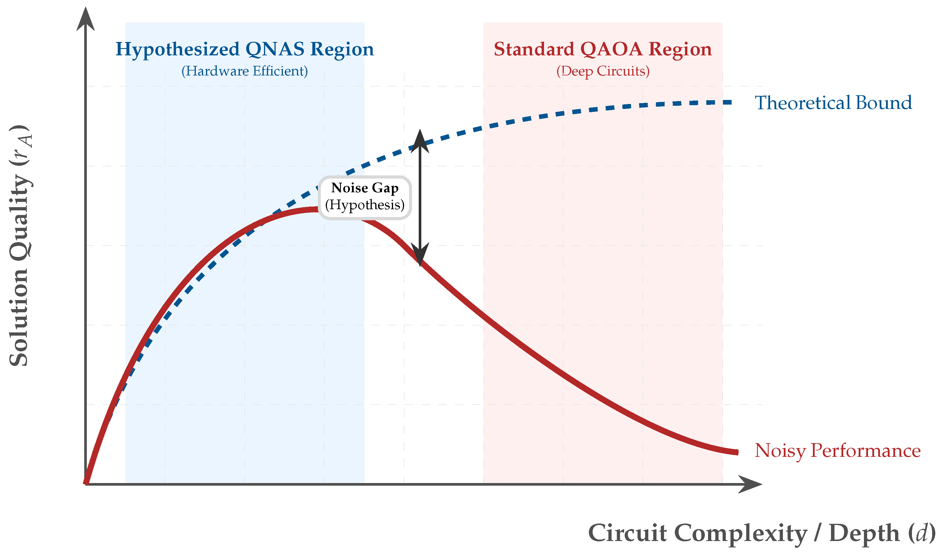
Our proposal (See Figure 1) is based on a direct comparison between the previously mentioned QAOA and the Quantum Neural Architecture Search (QNAS), which relies on evolutionary computing strategies to discover solutions to a specific problem. Several works, such as those presented in [8,9,10], employ different evolutionary techniques, as well as other approaches, such as reinforcement learning [3,11], for the automatic design of ansatzes.
However, a direct comparison of the functioning of heuristic approaches, such as QAOA, and automatic design strategies, such as QNAS, remains unexplored for well-defined problems, such as the MaxCut problem presented here.
An important remark is that, even though this study is related to the MaxCut problem, it can itself be viewed as part of a more general approach, since QNAS is well known for creating the search for potential Quantum Neural Network (QNN) architectures. A QNN can be represented as a VQC, which is itself a VQA.
This paper is organized as follows. Section 2 presents the theoretical framework, including the MaxCut problem formulation, the QAOA algorithm and its complexity analysis, and the QNAS approach based on NSGA-II. Section 3 details the experimental methodology, including the deployment environment, graph dataset construction, noise model specification, and performance metrics. Section 4 reports the results across ideal and noisy conditions, stratified by graph topology. Finally, Section 5 summarizes the findings and provides directions for future work.

2. Theoretical Background

2.1. Formulation of MaxCut Problem

The formal definition of the MaxCut problem [12] can be summarized by taking into account an undirected graph G = ( V , E ) with a set of vertices V and edges E. The objective is to find a partition of V into two disjoint sets, S and S c = V S , that maximizes the number of edges between them. The cut value is defined as follows:
Cut ( S ) = | { ( i , j ) E : i S , j S c } |
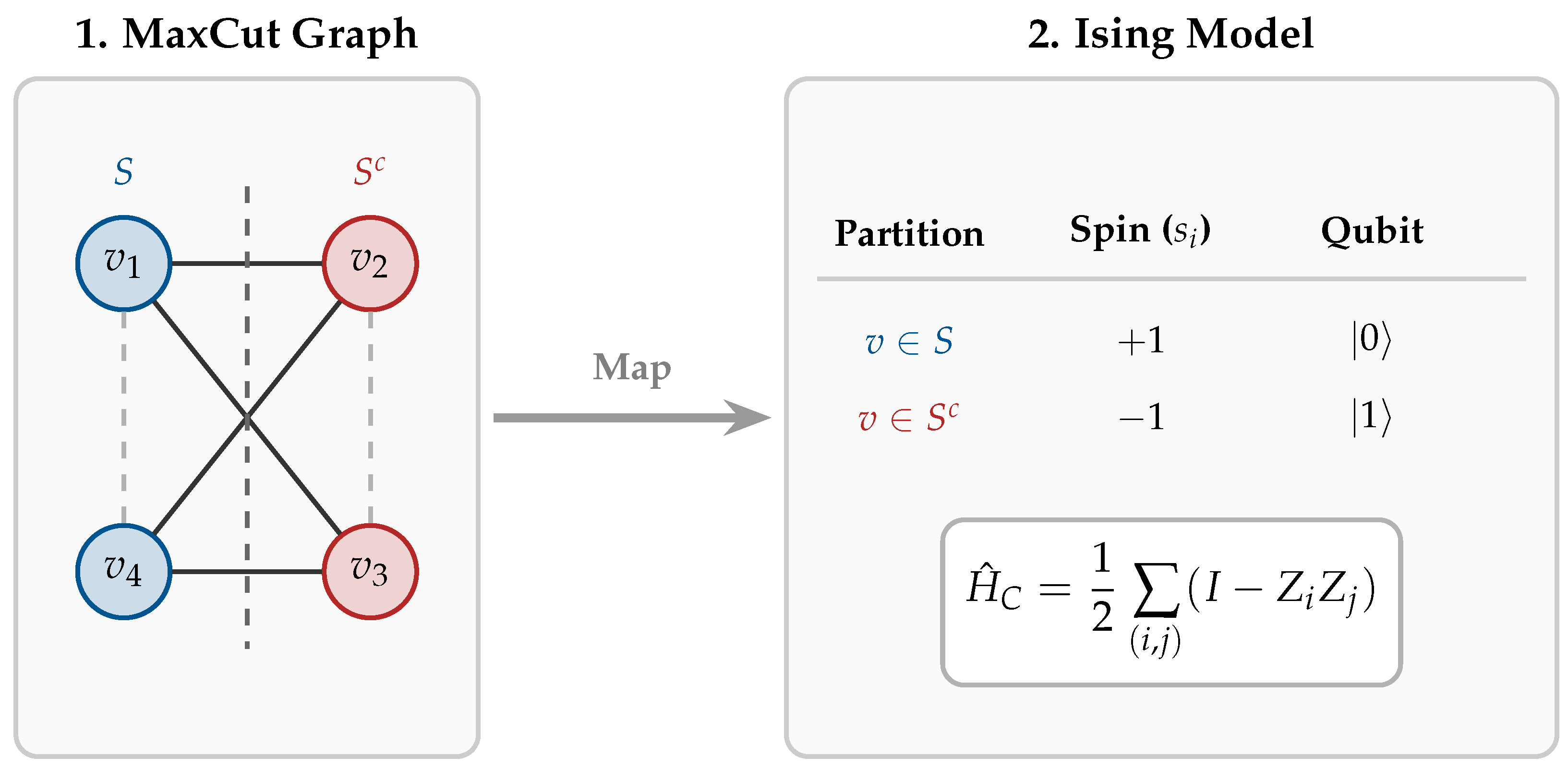
This problem can be mapped to find the ground-state in an Ising Hamiltonian (see Figure 2), since the two are isomorphic. We assign a spin variable s i { + 1 , 1 } to each vertex i, where s i = + 1 indicates i S and s i = 1 indicates i S c . The cost function becomes:
C ( s ) = 1 2 ( i , j ) E ( 1 s i s j )
This formulation relies on the fact that s i s j = 1 when vertices i and j are in different partitions, and s i s j = + 1 when they are in the same partition. By mapping s i σ i z , where σ z is the Pauli z–matrix, we obtain the Hamiltonian H C :
H C = 1 2 ( i , j ) E ( I σ i z σ j z )
The ground state of H C corresponds to the maximum cut. The measurement outcome z { 0 , 1 } n in the computational basis is interpreted as a bit-string, where qubit i in state | 0 corresponds to i S and | 1 to i S c .
An auxiliary metric called approximation ratio can be defined as:
r A = C ( z measured ) C
where C is the value of the optimal cut, and r A is a standard metric used to evaluate the quality of a solution provided by an optimization algorithm relative to the best possible (optimal) solution.

2.2. Quantum Approximate Optimization Algorithm (QAOA)

QAOA is a heuristic algorithm inspired by the adiabatic theorem [13] that, as stated previously, was handcrafted to provide solutions to combinatorial optimization problems [14]. This solution method consists of two elementary components of an ansatz, a cost Hamiltonian U C ( γ k ) = e i γ k H c and a mixer operator U M ( β k ) = e i β k H M . The cost part of the Hamiltonian ensures that the max-cut is evaluated; the mixer part, instead, ensures that the state being evaluated changes and that the algorithm does not fall into a local minimum. The proposed solution takes the following form:
| ψ ( γ , β ) = U M ( β p ) U C ( γ p ) U M ( β 1 ) U C ( γ 1 ) | + n ,
where γ = ( γ 1 , , γ p ) and β = ( β 1 , , β p ) are variational parameters (rotation angles), and | + = 1 2 ( | 0 + | 1 ) is the uniform superposition state. The notation | + n represents the tensor product of n qubits, each in the | + state.
The operators are applied sequentially from right to left, beginning with state preparation and then alternating p layers of cost and mixer unitaries. Each U C ( γ k ) encodes the problem Hamiltonian (Equation (3)), while U M ( β k ) = i = 1 n q e i β k X i implements the mixing part, where X i is the Pauli-X operator on qubit i.
The mixer operator U M acts by applying single-qubit Pauli-X rotations to each qubit, U M induces transitions between computational basis states, ensuring that the algorithm can escape local minima. This property guarantees that, as the number of layers p increases, the algorithm can, in principle, approximate the global optimum. U M also corresponds to the initial Hamiltonian H M = i X i , whose ground state is the uniform superposition | + n , the starting point from which the system evolves toward the ground state of the cost Hamiltonian H C .
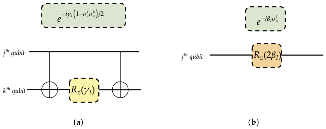
From Equation (5), it is possible to note that the function depends on a parameter p, which is usually referred to as the number of layers of the ansatz. However, it can be seen that all layers have a cost part and a mixer part; therefore, the number of layers is 2 p . A more visual representation of the structure of each layer in QAOA is shown in Figure 3.

Complexity Analysis of QAOA

The implementation cost of QAOA is dominated by the unitary cost U C . Since H C contains terms of the form Z i Z j , implementing U C requires one to realize the unitary e i γ Z i Z j for every edge ( i , j ) E . Standard decomposition requires two CNOT gates and one R z rotation [15]:
e i γ Z i Z j CNOT i j · R z ( 2 γ ) j · CNOT i j
Consequently, a single layer ( p = 1 ) requires 2 | E | CNOT gates plus n single-qubit gates for the mixer. For a complete graph K n , where | E | = n ( n 1 ) / 2 , the total CNOT count for depth p is
N CNOT p · n ( n 1 ) Θ ( p n 2 )
This quadratic scaling with system size n is the primary limitation of QAOA in the NISQ era, as error rates on CNOT gates ( 2 q -gates) ( ϵ 2 q 10 2 ) are approximately one order of magnitude higher than single-qubit gates ( ϵ 1 q 10 3 ) on current superconducting platforms.
For any graph G with determined depth p, QAOA provides a polynomial-time approximation algorithm for MaxCut. While the approximation ratio depends on p and graph topology, work by [16] proved that for p = 1 , QAOA achieves an approximation ratio of at least r A = 0.6924 for any 3-regular graph. Numerical evidence suggests that as p increases, QAOA can approach or exceed the Goemans–Williamson bound ( α 0.878 ) for specific graph families [17,18], though this remains an open theoretical question. However, this guarantee comes with the restriction that the parameters γ , β must be optimally chosen [19].

2.3. Quantum Neural Architecture Search (QNAS)

On the other side of our proposal, QNAS optimizes the architecture A (topology and gate selection), and it also optimizes the variational parameters (see Figure 4) θ for that specific architecture.
We can think of this as a Multi-Objective Optimization (MOO) problem:
min A S F ( A ) = ψ A ( θ ) | H C | ψ A ( θ ) , C ( A )
where:
  • S is the search space of possible circuits. In this approach, it is described as an integer list.
  • C ( A ) is the complexity cost referred to the potential hardware implementation.
  • θ denotes the parameters obtained via classical optimization (in our experimentation, we used (L-BFGS-B) [20] with 100 iterations).
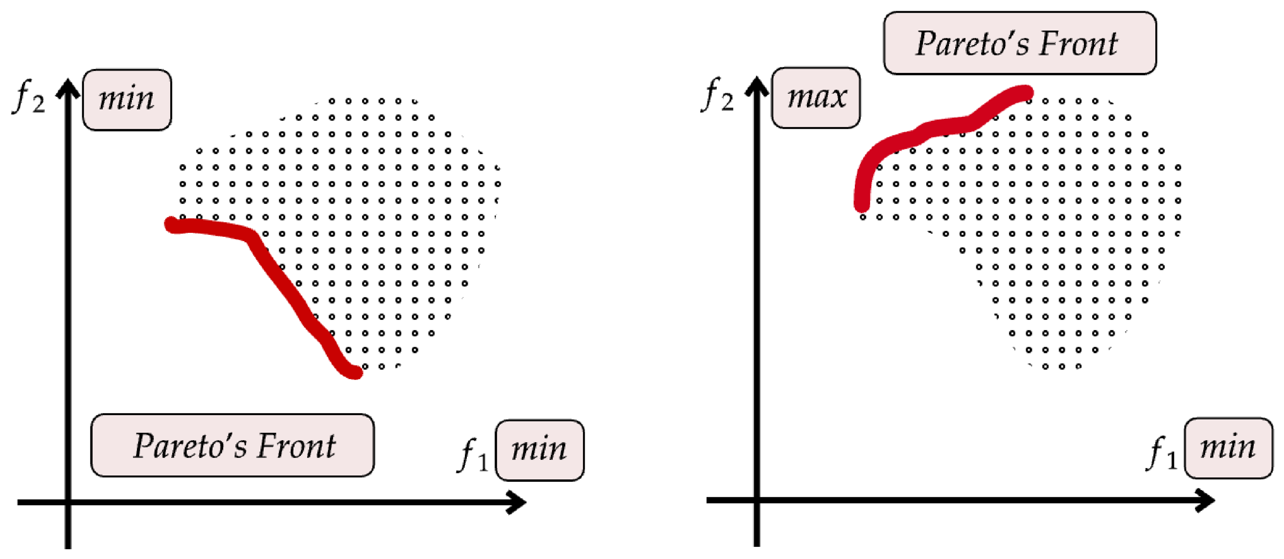
The objectives are conflicting (see Figure 5): increasing circuit depth generally improves expressibility (reducing the first objective) but increases complexity (increasing the second objective). The solution to this MOO problem is not a single architecture but a Pareto Front, a set of architectures where no objective can be improved without degrading another.

Evolutionary Search via NSGA-II

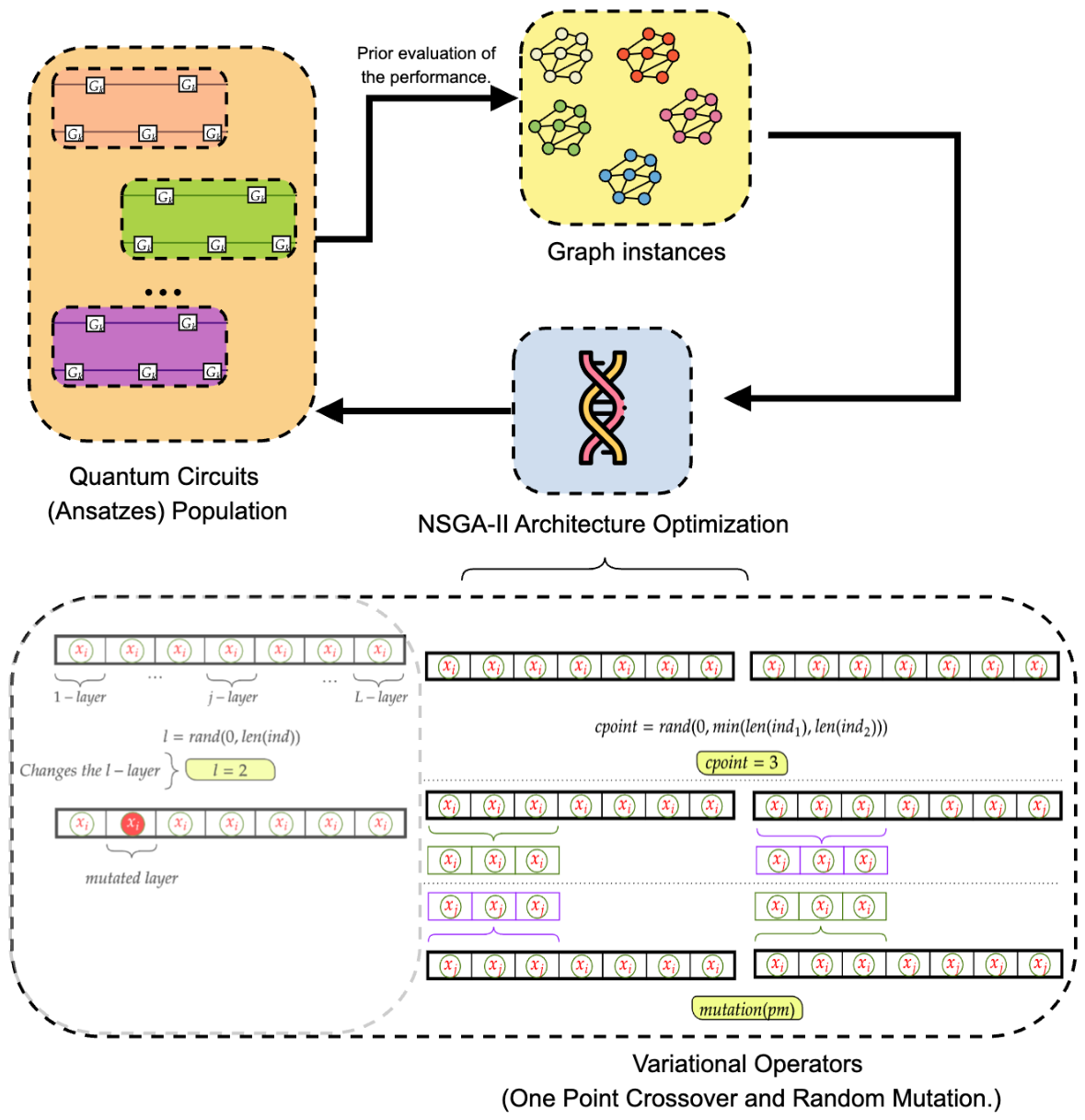
We employ the NSGA-II proposed by [21] to conduct the optimization of the architectures/topologies. NSGA-II works by creating a population of candidate architectures and evolving them through variational operators (selection, crossover, and mutation).
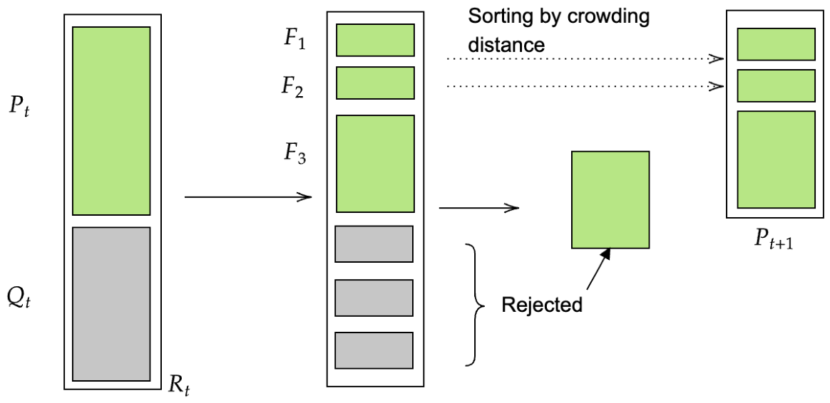
The functioning of NSGA-II under our proposal is defined in Algorithm 1, and illustrated in Figure 6 as a direct extrapolation of the original [21] reference.
Algorithm 1 NSGA-II for QNAS. A direct translation of the original algorithm [21] using the notation for the examined problem.
1: Initialize population P 0 of N random architectures
2: for generation g = 1 to G max  do
3:     for each architecture A P g  do
4:        Train parameters θ ( A ) via L-BFGS-B (inner loop)
5:        Evaluate objectives: f 1 ( A ) = H C A , f 2 ( A ) = C ( A )
6:     end for
7:     Perform non-dominated sorting on P g to assign ranks
8:     Calculate crowding distance for each architecture
9:     Generate offspring Q g via tournament selection, crossover, mutation
10:   Combine P g Q g and select best N for P g + 1
11: end for
12: return Pareto front from final population P G max
Selection is based on two criteria:
  • Pareto front rank: Solutions that are not dominated by any other solution receive Rank 1, and so forth. This stratification ensures convergence toward the true Pareto front.
  • Crowding distance: To preserve diversity, the algorithm prefers solutions that are in less crowded regions of the objective space. The crowding distance d i for individual i is calculated as:
    d i = m = 1 M f m ( i + 1 ) f m ( i 1 ) f m max f m min
    where M is the number of objectives, and ( i 1 ) , ( i + 1 ) denote the neighboring solutions in objective space sorted by f m . This prevents convergence to a single point on the front and ensures exploration of the entire trade-off surface.

3. Methodology

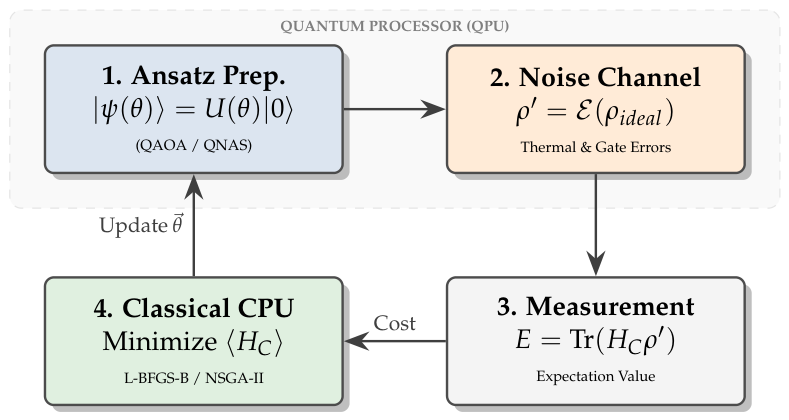
To create a fair benchmark for the proposed approaches, we developed a framework using Qiskit, a state-of-the-art Python (3.11.14) library for conducting real and simulated quantum executions. However, it is also important to illustrate the process that is being made in the execution of a VQA in a QC where the evaluation of the algorithm is being made (see Figure 7 and Figure 8).

3.1. Deployment Details

All quantum circuits were constructed, transpiled, and simulated using the IBM Qiskit SDK (version 0.44.0) with Qiskit Aer (version 0.12.2). Noiseless expectation values were obtained from statevector simulation, while the effect of noise was incorporated through the analytical fidelity model described in Section 3.4 (Equation (13)), which combines r A , ideal with an estimated circuit fidelity F est derived from the gate counts and per-gate error rates of Table 1.
To ensure reproducibility, we fixed the following environment parameters:
  • All circuits were transpiled (an important remark is that transpilation, which is commonly known as an optimization method for the circuits to be more efficient does not interfere with the QNAS approach since transpilation relies on the logic, while QNAS relies on the architecture of the circuit) to a standard basis gate set { R z , X , X , CNOT } using optimization level 3 (optimization_level = 3) to minimize swap gates excessive presence before noise injection.
  • For QAOA, we employed the L-BFGS optimizer (100 iterations). For the QNAS evolutionary loop, we implemented a custom NSGA-II genetic algorithm.
  • Fixed seeds were used for both graph generation (networkx) and quantum circuit initialization.

3.2. Structure of the Proposed Graphs for MaxCut Problem

We generated a dataset composed of 490 graphs from different distributions that may represent different physical phenomena. Our proposed graph distributions can be summarized as follows:
  • Random network graphs: We used the Erdös–Rényi model as a baseline to tackle problems without apparent structure.
  • Complex networks: In this case, we used Barabási–Albert and Watts–Strogatz models. The former is known for generating scale-free networks. All of them are common in real-world network analysis.
  • Regular graph distributions: We used a cycle graph, which models only local connectivity; a grid, which simulates problems with strong locality; a complete graph, which represents the case where the graph has maximum interaction density; and a star, which is a centralized graph.

QNAS Encoding Scheme

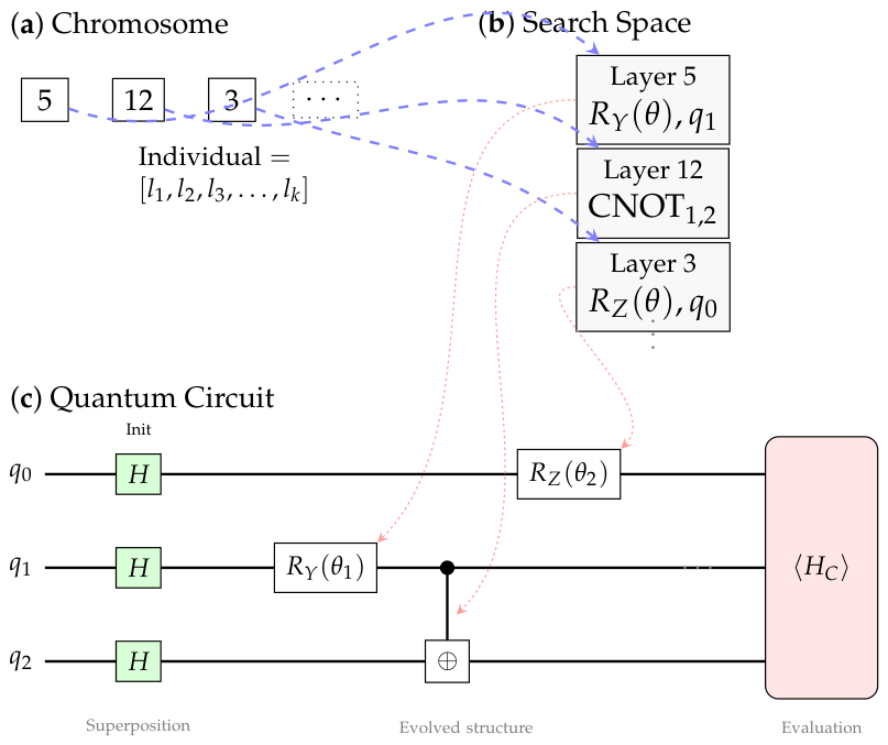
To codificate each candidate circuit, a variable-length chromosome was proposed (Figure 9a):
Individual = [ l 1 , l 2 , , l k ]
where each gene l i { 0 , 1 , , | S | 1 } indexes. The search space S is composed of atomic layers that include single-qubit rotation gates { R x , R y , R z , H } and two-qubit entangling gates { C N O T } , which are applied across all feasible qubit combinations. This representation facilitates the evolution of circuit topology and depth within the NSGA-II framework.
It is important to note that the list codification depends on the initial configuration used to generate the search space; that is, for a particular quantum computer, restrictions can be added to the search space, allowing a custom design for that hardware. This is particularly relevant since one of the capabilities we need to fight back is the lack of complete connectivity in real QCs.
An important clarification is that NSGA-II was executed independently for each graph instance, meaning that the architecture optimization was made to each specific problem. We acknowledge that this introduces additional computational overhead relative to QAOA, which uses a fixed ansatz structure across all instances. The cost of the evolutionary search is discussed in terms of the total number of circuit evaluations in Section 4.
The search space S consists of | S | = 7 atomic operations: parameterized single-qubit rotations ( R x , R y , R z ), the fixed Hadamard gate (H), linear nearest-neighbor CNOTs, circular CNOTs, and problem-specific Z Z interaction layers.
Experiment Hyperparameters: The NSGA-II algorithm was executed with a population size of N = 30 over a maximum of G max = 50 generations. The variational operators employed a single-point crossover with probability p c = 0.7 and random mutation with probability p m = 0.3 .

3.3. Noise Models and Their Importance in the Search

As previously stated, QCs tend to have more errors due to coherence issues and other physical factors. In this paper, we analyze the VQCs under varying noise conditions. To achieve this, we avoided simple depolarizing models in favor of a physically motivated noise model applied via Qiskit Aer simulator. The evolution of the density matrix ρ , which is a generalization of the state-vector approach and a representation of a VQC/VQA, is then governed by the operator-sum representation E ( ρ ) = k E k ρ E k , where E k corresponds to the basis (in this scenario, the computational basis) where the state is described. We modeled three distinct error channels applied sequentially to every operation in the circuit:

3.3.1. Gate Error Model

Gate errors were modeled using the depolarizing channel formalism, which approximates the complex error processes in physical devices. Under this model, a quantum state ρ subjected to a depolarizing channel with error probability p evolves as follows:
E ( ρ ) = ( 1 p ) ρ + p d 2 1 P I P ρ P
where d is the Hilbert space dimension, and P ranges over the Pauli group excluding identity. (We use the convention where p represents the total depolarizing probability, distributed uniformly across d 2 1 non-identity Pauli operators, consistent with Qiskit Aer v0.12.2’s depolarizing_error(p, num_qubits) implementation. Note that for single-qubit gates, e.g., ( d = 2 ), each Pauli error has a probability of p / 3 ; for two-qubit gates, e.g, ( d = 4 ), it is p / 15 .) The error rates employed in this study are summarized in Table 1.
Table 1. Noise Model Parameters. Error rates calibrated against IBM Eagle/Heron processor specifications. The depolarizing model provides an estimate of gate-fidelity loss by distributing errors uniformly across Pauli channels.
Error SourceSymbolValuePhysical Mechanism
Single-qubit gate error p 1 q 1.0 × 10 3 Depolarizing channel applied after each R x , R y , R z rotation; models pulse calibration drift and decoherence during gate execution.
Two-qubit gate error p 2 q 1.0 × 10 2 Depolarizing channel on both qubits post-CNOT/CZ; captures crosstalk, residual ZZ coupling, and extended gate duration effects.
Readout error p ro 2.0 × 10 2 Classical bit-flip confusion matrix; models resonator thermal population, insufficient integration time, and state relaxation during measurement.
The order-of-magnitude disparity between p 1 q and p 2 q reflects the fundamental difficulty of implementing high-fidelity entangling operations, which require precise control of inter-qubit coupling while suppressing parasitic interactions. This asymmetry motivates the complexity weighting scheme introduced in Section 3.4.
An important remark is that the depolarizing channel does not improve the performance of VQAs directly. However, QNAS benefits indirectly from noise through two mechanisms. First, during the NSGA-II search, decoherence penalizes complex circuits in the fitness evaluation via the fidelity term in r eff (Equation (13)). The Pareto-based selection pressure in NSGA-II implicitly suppresses deep architectures during evolution, since circuits exceeding a complexity threshold where fidelity decay dominates any marginal improvement in expressibility are outperformed on both objectives by more compact alternatives.

3.3.2. Readout Error Model

Measurement errors were implemented using a classical confusion matrix M applied to the ideal measurement outcome distribution:
p noisy = M · p ideal , M = 1 p ro p ro p ro 1 p ro
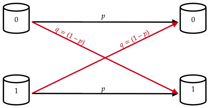
where p ro = 0.02 represents the probability of a bit-flip error during the measurement process (see Figure 10). This symmetric error model assumes equal misclassification rates for | 0 | 1 and | 1 | 0 transitions.

3.3.3. Discussion: Impact of Different Noise Channels

The depolarizing channel employed in this study distributes errors uniformly across all Pauli operators, constituting the worst-case scenario for a given error probability p.
Phase damping (dephasing) is a unital channel characterized by Kraus operators E 0 = 1 0 0 1 λ and E 1 = 0 0 0 λ , where λ is related to the T 2 coherence time. This channel destroys off-diagonal coherences while preserving diagonal populations. Since the MaxCut cost Hamiltonian H C = 1 2 ( I Z i Z j ) depends exclusively on diagonal elements of the density matrix in the computational basis, phase damping has a reduced impact on the expectation value H C compared to depolarizing noise.
Amplitude damping models energy relaxation ( T 1 decay) and is described by Kraus operators E 0 = | 0 0 | + 1 γ | 1 1 | and E 1 = γ | 0 1 | , where γ = 1 exp ( t gate / T 1 ) . Unlike the depolarizing and dephasing channels, amplitude damping is non-unital: it does not preserve the maximally mixed state, instead driving the system asymptotically toward | 0 n . For the MaxCut problem, we define an initial setup which corresponds to placing all vertices in the same partition (a trivial cut with C = 0 ).
For equivalent error probabilities, the expected degradation hierarchy is depolarizing ≥ amplitude damping > phase damping. The crossover point identified at n 12 (discussed in detail in Section 4) thus represents a pessimistic estimate under the depolarizing model; alternative channels would shift this threshold to equal or larger system sizes while preserving the qualitative advantage of QNAS over QAOA.

3.4. Performance Metrics

As described earlier, different types of gates correspond to different problems; in particular, assuming equal complexity is a mistake. To correct this, we define a weighted complexity metric that accounts for the different set of quantum gates:
C = N 1 q + w · N 2 q , w = p 2 q p 1 q = 10
where N 1 q and N 2 q denote the total number of single-qubit and two-qubit gates, respectively. The weighting factor w is derived directly from the error rate ratio.

Noise-Adjusted Approximation Ratio

Standard approximation ratios r A = C / C max are not effective for evaluating algorithms in high-noise regimes. In a physical system dominated by maximal decoherence (white noise), the quantum state becomes the maximally mixed state I / 2 n . For unweighted MaxCut, measuring this state yields a random cut, which corresponds to an expected approximation ratio of 0.5 .
To quantify the utility of a quantum circuit relative to this physical baseline, we define r e f f as the Noise-Adjusted Approximation Ratio:
r eff = r A , ideal · F est + 0.5 · ( 1 F est )
where r A , ideal is the noiseless approximation ratio derived from ideal simulation. F est exp [ ( p 1 q N 1 q + p 2 q N 2 q ) ] corresponds to the estimated circuit fidelity, calculated using the gate error rates ( p 2 q 10 2 ) and gate counts (N) specific to each ansatz. This constitutes a pessimistic bound on circuit fidelity, as it assumes independent depolarizing errors with no error cancellation or coherent recombination.
In the limit of perfect hardware ( F 1 ), r eff r A , ideal . As the circuit depth exceeds the coherence time ( F 0 ), the performance converges to the random guessing value of 0.5 . This allows us to identify the point where the algorithm becomes indistinguishable from noise.
The balance between C and r eff defines a Pareto frontier in the complexity–performance space. Circuits lying on this frontier represent optimal configurations where no improvement in r eff is achievable without increasing C, and vice-versa. In order to create fair comparisons the knee point of PF was taken into account.
We note that r eff is an estimate that combines the ideal approximation ratio from noiseless simulation with an analytical fidelity model. Another approach would be to report the directly simulated noisy approximation ratio obtained from Qiskit Aer.

4. Results

We benchmarked the standard QAOA with p = 5 against the adaptive QNAS. The choice of p = 5 was due to the fact that, theoretically, this depth provides sufficient expressibility to achieve approximation ratios r A > 0.90 , minimizing the underfitting errors typical of shallow circuits.
We selected p = 5 as a representative deep-circuit regime because it lies above the theoretical threshold for high approximation ratios on the tested graph sizes while remaining computationally tractable for full simulation across 490 instances. We acknowledge that intermediate depths ( p { 1 , 2 , 3 } ) may yield different complexity–performance trade-offs; in particular, a lower p would reduce the complexity gap between QAOA and QNAS. A systematic multi-depth analysis constitutes an immediate extension of this work that would strengthen the generalizability of the reported crossover behavior.
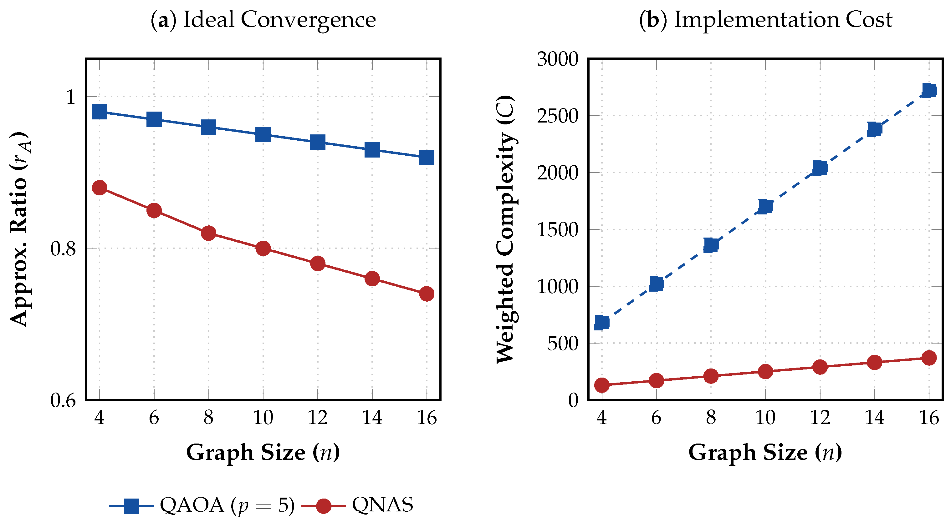
Figure 11a validates this theoretical premise. In noiseless simulations, QAOA ( p = 5 ) consistently delivers superior solution quality ( r A 0.92 for n = 16 ), outperforming the shallower structures discovered by QNAS. This confirms that, in an ideal fault-tolerant regime, depth is the primary driver of convergence.
However, Figure 11b exposes the implementation barrier. The Complexity of the p = 5 ansatz scales linearly but with a prohibitive slope. For n = 16 , the circuit requires approximately 2700 weighted operations to enforce the multilayered topology. In contrast, QNAS identifies hardware-efficient circuits with a complexity of ≈370, representing an 86 % reduction in gate resources while preserving structural connectivity.

4.1. What Solutions Are Really Feasible?

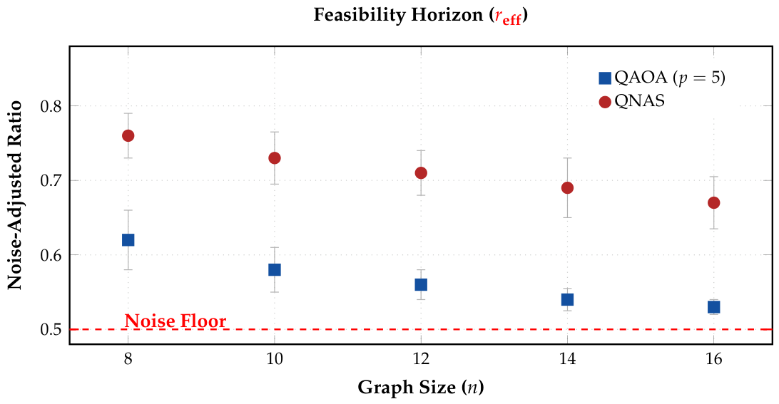
The discrepancy between theoretical potential and physical realization is quantified by the Noise-Adjusted Approximation Ratio ( r eff ). Table 2 presents the metrics for n = 16 . Despite QAOA showing a high ideal ratio, the estimated circuit fidelity drops to 6.6 % due to error accumulation. This forces the effective ratio to converge toward the random noise floor ( 0.5 ).
We observe a crossover at n 12 . Beyond this point (see Figure 12), the p = 5 ansatz enters a regime where adding depth destroys more information than it creates. QNAS, by sacrificing theoretical perfection for structural efficiency, maintains a clear optimization signal ( r eff > 0.65 ) well into the region where QAOA collapses.
The asymptotic behavior of both approaches can be characterized analytically from Equation (13). For QAOA, ( p = 5 ), and the estimated fidelity decays as F est = exp p 2 q · 2 p · n ( n 1 ) 2 , yielding F est 0.02 at n = 18 and F est 0.006 at n = 20 , which drives r eff . This degradation does not stabilize; it follows an exponential decay governed by the O ( n 2 ) gate count scaling. In contrast, QNAS circuits maintain bounded complexity independent of graph connectivity, with empirical values C < 500 across all tested system sizes. Extrapolating with C 400 gives F est 0.67 and r eff 0.74 × 0.67 + 0.5 × 0.33 0.66 , suggesting that QNAS performance stabilizes in the interval [ 0.60 , 0.66 ] as n increases beyond the tested range.
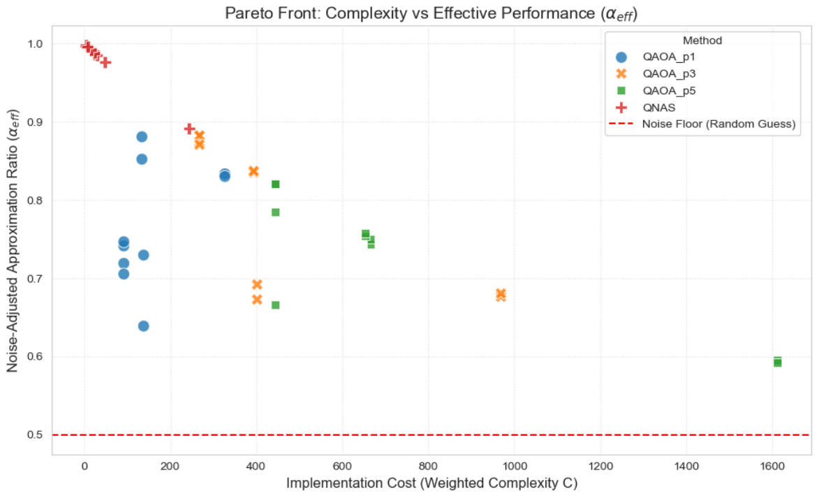
To create a fair comparison and test the hypothesis that smaller circuits exhibit greater noise resilience, we expanded our experiments to include QAOA at intermediate depths ( p { 1 , 3 } ). As illustrated in the Complexity–Performance Pareto Front (Figure 13), QAOA ( p = 1 ) reduces the structural complexity ( C 156 ) compared to the p = 5 regime ( C 763 ). However, an important remark is that it suffers from severe underfitting, achieving an effective approximation ratio of only r eff 0.76 . At the same time, QNAS strictly dominates the Pareto frontier. This suggests that the evolutionary approach consistently discovers more hardware-efficient architectures ( C 41 ) while approaching optimal theoretical values ( r eff 0.98 ). This small validation in a subset suggests that the superiority of QNAS is not merely an artifact of comparing against a deep, noise-sensitive ansatz.

4.2. Structural Analysis

We decomposed performance by a stratified description of the graph topology and density.

Topology Dependence

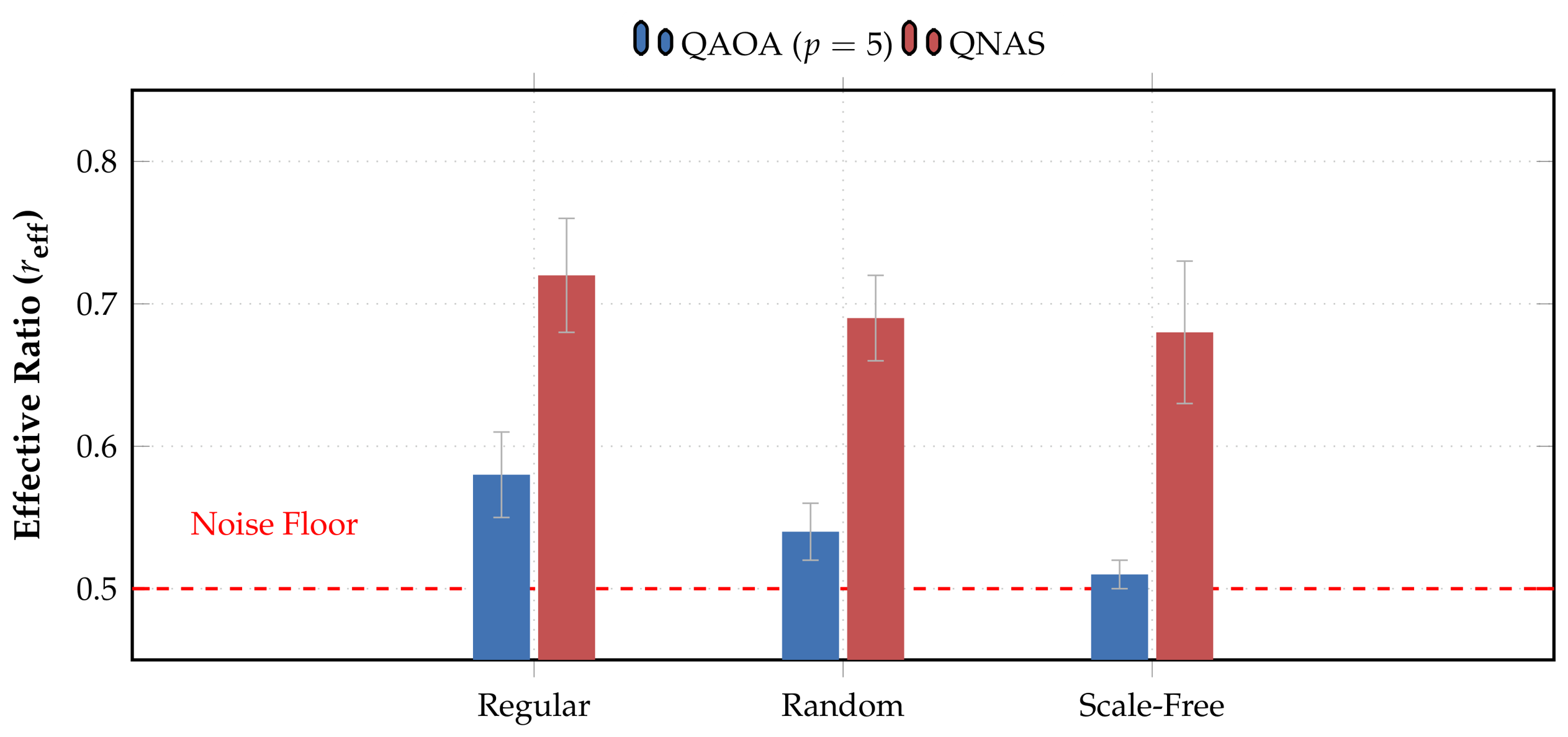
Figure 14 contrasts performance across three distinct graph classes. While QAOA ( p = 5 ) exhibits robustness in regular graphs ( d 2 4 ), its effective performance collapses on Scale-Free networks.QNAS excels here by pruning hub connections, preserving the global signal.
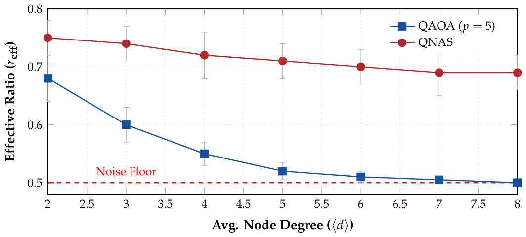
Finally, Figure 15 illustrates that, for fixed depth p, the circuit depth of QAOA scales linearly with average degree d . At d > 4 , error accumulation becomes critical. QNAS maintains a flat performance profile.

5. Conclusions

In this work, we addressed ansatz selection for Variational Quantum Algorithms by comparing a heuristic strategy (QAOA, p = 5 ) with an evolutionary architecture search (QNAS). Our research, performed across 490 graph instances under noise models, reveals a serious trade-off between theoretical expressibility and physical implementability in the NISQ era.
While the QAOA ansatz demonstrated better convergence capabilities in noiseless simulations ( r A > 0.90 ), confirming that depth is the key element to the characterization of solution quality in ideal systems, its practical utility is strictly bounded by hardware coherence. At system size n 12 solutions were comparable. Beyond this threshold, the linear scaling of the standard ansatz imposes a complexity penalty ( C > 2700 for n = 16 ) that drives the effective approximation ratio to the random noise floor ( r eff 0.5 ). In contrast, QNAS demonstrated remarkable structural resilience. By decoupling circuit complexity from graph connectivity, the evolutionary approach reduced gate requirements by approximately 86 % compared to the p = 5 baseline. Through the ability to selectively delete non-essential entanglement—QNAS maintained inside a valid optimization ( r eff > 0.65 ) regime.
These findings suggest that simply increasing circuit depth to improve theoretical convergence is a counterproductive strategy without error correction. Instead, resources should be directed toward adaptive, hardware-aware ansatz compilation. Future work will extend the benchmark to larger systems ( n > 20 ) using tensor network simulators to validate the analytical extrapolation presented in Section 4 and further explore the limits of topological pruning. Second, the noise model will be generalized to include amplitude damping ( T 1 relaxation) and phase damping ( T 2 dephasing) channels independently and in combination, using device-specific parameters from current IBM quantum processors to quantify how unital versus non-unital noise modifies the Pareto front topology discovered by QNAS and the degradation profile of QAOA.
Furthermore, deep circuits ( p = 5 ) collapse under decoherence, while shallow circuits ( p = 1 ) suffer from extreme underfitting. QNAS bypasses this limitation, showing that dynamic, hardware-aware ansatz compilation is an alternative superior to static topologies in the current NISQ era.

Author Contributions

Conceptualization, E.I.J.C. and H.T.-M.; methodology, E.I.J.C.; software, E.I.J.C.; validation, E.I.J.C., H.T.-M., and E.M.-M.; formal analysis, E.I.J.C.; investigation, review and editing, E.I.J.C., H.T.-M., and E.M.-M.; visualization, E.I.J.C.; supervision, H.T.-M. and E.M.-M. All authors have read and agreed to the published version of the manuscript.

Funding

This research was funded by Secretaría de Ciencia, Humanidades, Tecnología e Innovación (SECITHI) through BECAS NACIONALES 2023 CVU: 1083296.

Data Availability Statement

The data that support the findings of this study are available from the corresponding author E.I.J.C., upon reasonable request.

Acknowledgments

During the preparation of this manuscript, the authors used Grammarly for the purposes of enhancing the English communication.

Conflicts of Interest

The authors declare no conflicts of interest.

Abbreviations

The following abbreviations are used in this manuscript:
NISQNoisy Intermediate-Scale Quantum
VQAVariational Quantum Algorithm
VQCVariational Quantum Circuit
QAOAQuantum Approximate Optimization Algorithm
QNASQuantum Neural Architecture Search
NSGA-IINon-dominated Sorting Genetic Algorithm II
VQEVariational Quantum Eigensolver
NASNeural Architecture Search
MOOMulti-Objective Optimization
CNOTControlled-NOT gate
KLKullback–Leibler
L-BFGS-BLimited-memory Broyden–Fletcher–Goldfarb–Shanno with Bound constraints
ERErdős–Rényi
BABarabási–Albert
WSWatts–Strogatz

References

  1. Preskill, J. Quantum computing in the NISQ era and beyond. Quantum 2018, 2, 79. [Google Scholar] [CrossRef] [Scilit]
  2. Cerezo, M.; Arrasmith, A.; Babbush, R.; Benjamin, S.C.; Endo, S.; Fujii, K.; McClean, J.R.; Mitarai, K.; Yuan, X.; Cincio, L.; et al. Variational quantum algorithms. Nat. Rev. Phys. 2021, 3, 625–644. [Google Scholar] [CrossRef] [Scilit]
  3. Chen, S.Y.-C.; Huang, C.-M.; Hsing, C.-W.; Goan, H.-S.; Kao, Y.-J. Variational quantum reinforcement learning via evolutionary optimization. Mach. Learn. Sci. Technol. 2022, 3, 015025. [Google Scholar] [CrossRef] [Scilit]
  4. Sim, S.; Johnson, P.D.; Aspuru-Guzik, A. Expressibility and entangling capability of parameterized quantum circuits for hybrid quantum-classical algorithms. Adv. Quantum Technol. 2019, 2, 1900070. [Google Scholar] [CrossRef] [Scilit]
  5. McClean, J.R.; Boixo, S.; Smelyanskiy, V.N.; Babbush, R.; Neven, H. Barren plateaus in quantum neural network training landscapes. Nat. Commun. 2018, 9, 4812. [Google Scholar] [CrossRef] [Scilit] [PubMed]
  6. Cerezo, M.; Sone, A.; Volkoff, T.; Cincio, L.; Coles, P.J. Cost function dependent barren plateaus in shallow parametrized quantum circuits. Nat. Commun. 2021, 12, 1791. [Google Scholar] [CrossRef] [Scilit] [PubMed]
  7. Kim, Y.; Eddins, A.; Anand, S.; Wei, K.X.; van den Berg, E.; Rosenblatt, S.; Nayfeh, H.; Wu, Y.; Zaletel, M.; Temme, K.; et al. Evidence for the utility of quantum computing before fault tolerance. Nature 2023, 618, 500–505. [Google Scholar] [CrossRef] [Scilit] [PubMed]
  8. Li, Y.Y.; Liu, R.J.; Hao, X.B.; Shang, R.H.; Zhao, P.X.; Jiao, L.C. EQNAS: Evolutionary quantum neural architecture search for image classification. Neural Netw. 2023, 168, 471–483. [Google Scholar] [CrossRef] [Scilit] [PubMed]
  9. Zhu, X.; Hou, X. Quantum architecture search via truly proximal policy optimization. Sci. Rep. 2023, 13, 5157. [Google Scholar] [CrossRef] [Scilit] [PubMed]
  10. Altares-López, S.; Ribeiro, A.; García-Ripoll, J.J. Automatic design of quantum feature maps. Quantum Sci. Technol. 2021, 6, 045015. [Google Scholar] [CrossRef] [Scilit]
  11. Kuo, E.-J.; Fang, Y.-L.L.; Chen, S.Y.-C. Quantum architecture search via deep reinforcement learning. arXiv 2021, arXiv:2104.07715. [Google Scholar] [CrossRef] [Scilit]
  12. Karp, R.M. Reducibility among combinatorial problems. In Complexity of Computer Computations; Springer: Berlin/Heidelberg, Germany, 1972; pp. 85–103. [Google Scholar] [CrossRef] [Scilit]
  13. Kadowaki, T.; Nishimori, H. Quantum annealing in the transverse Ising model. Phys. Rev. E 1998, 58, 5355. [Google Scholar] [CrossRef] [Scilit]
  14. Farhi, E.; Neven, H. Classification with quantum neural networks on near term processors. arXiv 2018, arXiv:1802.06002. [Google Scholar] [CrossRef] [Scilit]
  15. Crooks, G.E. Performance of the quantum approximate optimization algorithm on the maximum cut problem. arXiv 2018, arXiv:1811.08419. [Google Scholar] [CrossRef] [Scilit]
  16. Farhi, E.; Goldstone, J.; Gutmann, S. A quantum approximate optimization algorithm. arXiv 2014, arXiv:1411.4028. [Google Scholar] [CrossRef] [Scilit]
  17. Wurtz, J.; Love, P. MaxCut quantum approximate optimization algorithm performance guarantees for p > 1. Phys. Rev. A 2021, 103, 042612. [Google Scholar] [CrossRef] [Scilit]
  18. Basso, J.; Farhi, E.; Marwaha, K.; Gutmann, S.; Neven, H. The quantum approximate optimization algorithm at high depth for MaxCut on large-girth regular graphs and the Sherrington-Kirkpatrick model. arXiv 2022, arXiv:2110.14206. [Google Scholar]
  19. Brandão, F.G.S.L.; Broughton, M.; Farhi, E.; Gutmann, S.; Neven, H. For fixed control parameters the quantum approximate optimization algorithm’s objective function value concentrates for typical instances. arXiv 2018, arXiv:1812.04170. [Google Scholar]
  20. Byrd, R.H.; Lu, P.; Nocedal, J.; Zhu, C. A limited memory algorithm for bound constrained optimization. SIAM J. Sci. Technol. 1995, 16, 1190–1208. [Google Scholar] [CrossRef] [Scilit]
  21. Deb, K.; Pratap, A.; Agarwal, S.; Meyarivan, T. A fast and elitist multiobjective genetic algorithm: NSGA-II. IEEE Trans. Evol. Comput. 2002, 6, 182–197. [Google Scholar] [CrossRef] [Scilit]
Figure 1. Hypothesized performance trade-off in NISQ devices. The blue region corresponds to the regime targeted by QNAS. The red region indicates the standard QAOA regime.
Mca 31 00078 g001
Figure 2. Visual mapping of the MaxCut problem. Vertices are partitioned into two sets (S and S c ), which correspond to spin states ± 1 and qubit basis states | 0 , | 1 .
Mca 31 00078 g002
Figure 3. The structure of the QAOA ansatz layers, generalizable to n qubits. (a) The cost layer U C ( γ ) implements the problem Hamiltonian via Z Z -interaction gates between connected qubits, with each edge requiring two CNOT gates and one R z rotation. (b) The mixer layer U M ( β ) applies single-qubit R x rotations parameterized by β to each qubit, implementing Pauli-X rotations.
Mca 31 00078 g003
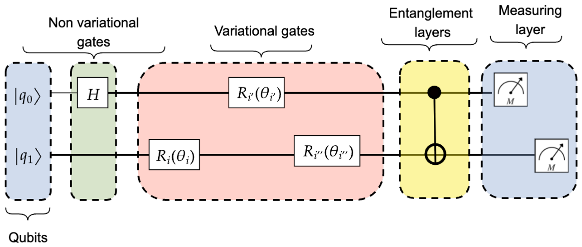
Figure 4. Typical structure of a VQC. State preparation and parameterized gates—non-variational gates initialize the qubits, followed by variational rotation gates R i ( θ ) , whose parameters are optimized classically. Entanglement and measurement—two-qubit entangling gates create correlations between qubits, and the measurement layer projects the quantum state onto the computational basis to evaluate the cost function.
Mca 31 00078 g004
Figure 5. An illustration on conflicting objectives, a condition which is necessary to conduct a multiobjective optimization, in the proposal case f 1 expressibility and f 2 complexity .
Mca 31 00078 g005
Figure 6. Graphical representation of Algorithm 1; the total population P t Q t is sorted by Pareto Front (PF) ranks, and then that set of PF is sorted by crowding distance—a metric that enhances the diversity of the selected population, ensuring that the solutions are diverse and therefore more representative of the Pareto front.
Mca 31 00078 g006
Figure 7. Complete overview of the optimization process using QNAS approach. In the evaluation of the performance of each dataset, noise was taken into account. Circuit representation used merely for visualization purposes.
Mca 31 00078 g007
Figure 8. Structure of the execution of a VQA under noise conditions, this kind of algorithm is not purely quantum since the optimization of the variational parameters is being assisted by a classical CPU.
Mca 31 00078 g008
Figure 9. QNAS encoding and circuit synthesis. (a) Chromosome representation with variable length k. (b) Search space indexed by genes. (c) Synthesized a circuit from a chromosome [5, 12, 3, …]. Dotted lines trace gene-to-gate mappings.
Mca 31 00078 g009
Figure 10. Classical visualization of readout errors in a computer. In traditional computers, these errors can be mitigated by redundancy, which is not possible in QCs. In the case of QCs, the translation is straightforward | 0 0 and | 1 1 .
Mca 31 00078 g010
Figure 11. The cost of depth. (a) In ideal conditions, QAOA ( p = 5 ) dominates due to high expressibility. (b) However, the associated hardware cost for n = 16 exceeds 2700 operations, creating a massive gap compared to the optimized QNAS.
Mca 31 00078 g011
Figure 12. Effective performance with 95 % confidence intervals. Red-dashed line marks the random guessing limit. QAOA converges to the noise floor with diminishing variance as system size increases.
Mca 31 00078 g012
Figure 13. Complexity–Performance Pareto Front. QNAS strictly dominates the optimal trade-off curve compared to QAOA evaluated at multiple depths ( p { 1 , 3 , 5 } ).
Mca 31 00078 g013
Figure 14. Topology Dependence. Mean effective performance. QAOA suffers critical degradation on Scale-Free graphs, approaching the noise floor, while QNAS adapts to the irregular structure.
Mca 31 00078 g014
Figure 15. Resilience to Density. Effective performance vs. average node degree ( n = 16 ). Increased connectivity degrades QAOA performance due to error accumulation, while QNAS remains stable.
Mca 31 00078 g015
Table 2. Performance Summary ( n = 16 ). QAOA ( p = 5 ) maximizes theoretical potential but fails to preserve the result under noise.
MetricQAOA ( p = 5 )QNAS
Ideal Ratio ( r A , ideal ) 0.92 0.74
Complexity Score (C)2720370
Est. Fidelity (F) 0.06 0.69
Effective Ratio ( r eff ) 0.53 (Noise) 0.67 (Signal)
Disclaimer/Publisher’s Note: The statements, opinions and data contained in all publications are solely those of the individual author(s) and contributor(s) and not of MDPI and/or the editor(s). MDPI and/or the editor(s) disclaim responsibility for any injury to people or property resulting from any ideas, methods, instructions or products referred to in the content.