Decision-Making for Secure and Stable Operation of Power Systems: A Multi-Scenario-Based Optimization Model

Abstract

In practical power system operation scenarios, extreme natural weather conditions and fluctuations at both the supply and demand sides pose significant challenges to the stable operation and the formulation of operational decision-making for power systems. Particularly in extreme scenarios involving faults, it may lead to power supply–demand imbalances and instability in the power system. To address this issue, this paper proposes a decision-making approach for the secure and stable operation of power systems using a multi-scenario-based optimization model. Initially, a joint scenario set is generated using historical operational data to accurately depict multiple complex scenarios. Building on this, a multi-scenario-based optimization model is constructed, with responses facilitated by flexible adjustment resources within the system. Considering the non-convex and nonlinear characteristics of the model, an improved Harris Hawks Optimization (HHO) algorithm is employed to search for the global optimal solution. Finally, a modified IEEE-33 bus test system is utilized to demonstrate the feasibility and effectiveness of the proposed method.

1. Introduction

Against the backdrop of constructing a next-generation power system, the installed capacity of renewable energy sources such as wind and photovoltaic power has witnessed rapid growth, leading to significant changes in the operational characteristics of the power system [1]; concurrently, the frequent occurrence of extreme events has exacerbated the mismatch between supply and demand on both the source and load sides of the power system, intensifying the challenges of ensuring power supply reliability [2,3]. Therefore, researching decision-making methods for the secure and stable operation of power systems under complex scenarios is an urgent requirement for the safe, economic, and efficient development of power systems following the integration of a high proportion of renewable energy sources [4].

In the realm of power system security, traditional network protection technologies mainly consist of static measures like intrusion detection systems and firewalls [5]; however, these technologies are confronted with challenges such as sophisticated and persistent threats. In response to potential disruptions that could impact power systems, scholars have put forward reliability assessments [6], defense tactics, and recovery strategies specifically tailored for the power system domain [7]. Nevertheless, these reactive defense measures find it difficult to counter all conceivable disruptive behaviors, and with the continual emergence of new types of disruptions, research has shifted towards proactive defense strategies to navigate the increasingly intricate security landscape. References [8,9] delve into how to devise disruptive scenarios for estimation models with vulnerabilities through techniques such as sparse reconstruction, robust regression, or tensor factorization under conditions where partial state information is unavailable. Reference [10] quantifies the detectability of disruptions by introducing metrics such as tensor state estimation frameworks and the Kullback–Leibler divergence, proposing more system-adaptive strategies for generating disruptive scenarios from both theoretical and practical standpoints. Although these methods identify system vulnerabilities from a disruption perspective, they have not yet established effective integrated protection mechanisms, making it challenging to directly meet security requirements. To address latency issues, recent endeavors in constructing defense mechanisms have integrated physical process prediction, state estimation, and control adjustments into a closed-loop regulation framework to achieve dynamic scenario adaptation and a coordinated response to disruptions. Reference [11] proposes multi-scale state stabilization mechanisms for distribution and wide-area power systems based on hybrid automata and probabilistic prediction and filtering fusion strategies, respectively. Reference [12] enhances the accuracy of abnormal state identification and improves the convergence effect of emergency response strategies by introducing innovative approaches such as generative adversarial learning and system-wide data integration techniques. These achievements indicate that the future development trend of disruption-resistant control is the deep integration of detection and control logic, thereby achieving a unified response to frequency disturbances and data anomalies.

Meanwhile, current resource optimization allocation in power systems typically employs scenario selection strategies to obtain typical scenarios to reduce model computational scale and facilitate solution finding. Reference [13] proposes a renewable energy scenario reduction method based on clustering and optimization algorithms, determining the number of clusters through data cleaning and clustering, and selecting typical scenarios using particle swarm optimization and genetic algorithms to generate typical scenarios reflecting regional characteristics. Reference [14] proposes a multi-stage nested reduction algorithm integrating recursive clustering, optimizing the scenario extraction process by incorporating an improved Wasserstein distance metric, and balancing accuracy, timeliness, and stability. Reference [15] constructs a comprehensive evaluation index system for typical day selection by comprehensively considering the total amount, distribution, typicality, and extremity characteristics of resources and loads, reducing selection errors. Reference [16] proposes a scenario reduction method combining improved k-means clustering with synchronous backward elimination and verifies its effectiveness using data from a provincial network in northwest China. Reference [17] proposes a joint extraction method based on local linear embedding, kernel density estimation, and the FP-growth algorithm for selecting typical scenarios in urban photovoltaic distribution networks and validates its low error using data from the Qingyuan distribution network in Guangdong Province. However, methods considering only typical scenarios suffer from the issue of extreme scenario information being easily overwhelmed [18], resulting in power system resource allocation failing to meet power supply reliability requirements. Therefore, considering the impact of extreme scenarios in resource optimization allocation to reduce scenario selection errors is fundamental to meeting power system supply reliability requirements. The current common approach involves initially selecting extreme scenarios through expert experience methods and combining them with typical scenarios to solve the optimization model, obtaining an initial power system optimization allocation plan; subsequently, based on this initial plan, whether the system meets power supply reliability requirements across all scenarios is analyzed. If it does, the optimal planning scheme is considered obtained; otherwise, all load shedding scenarios are added at once for a new round of resource allocation optimization [19]. However, this method suffers from issues of inaccurate extreme scenario identification and inefficient optimization model solving: in terms of extreme scenario identification, traditional scenario selection methods such as clustering and expert experience methods alone cannot accurately identify extreme scenarios, resulting in unreliable power system resource allocation optimization for extreme conditions [20]; in terms of computational efficiency, adding all load shedding scenarios at once leads to a large model scale and low computational efficiency. To address these shortcomings, domestic and foreign experts and scholars have researched a series of extreme scenario selection methods. Reference [21] proposes a long-time-scale system operation scenario generation method accounting for extreme meteorology, modeling meteorological factors based on the spatiotemporal distribution characteristics of extreme meteorological events, inserting multiple short-time-scale meteorological events into annual time series, and generating scenarios using a data-knowledge joint driving method. Reference [22] proposes a grid extreme operation scenario extraction method based on data mining and machine learning, identifying key variables, measuring contributions using the entropy weight method, and extracting edge outliers as extreme scenarios using weighted clustering. Reference [23] proposes a weighted clustering-based extreme operation scenario selection method, selecting typical grid operation scenarios using annual time series data of wind power and load, combined with time variation and correlation analysis, and identifying extreme scenarios from edge points far from cluster centers. Reference [24] proposes an extreme scenario selection method based on importance sampling and k-means clustering, extracting key physical information from a large number of simulated scenarios and applying it to two-stage stochastic economic dispatch calculations. Reference [25] proposes a closed-loop energy storage planning framework for full-scenario security, ensuring resource optimization, allocation security, and computational efficiency across all scenarios through a scenario ranking-guided update strategy, while further improving computational efficiency by generating an initial critical scenario set strategy based on self-organizing map neural networks and scenario key indicator ranking. In the context of constrained resource allocation in power systems, digital twin technology can rely on the full-element mapping of physical power systems to construct virtual twins, enabling real-time perception, online analysis, and dynamic simulation of the operational status of power systems [26]. It allows for lossless, high-fidelity simulation and deduction of various scenarios, including abnormal information transmission, fluctuations in renewable energy output, and extreme weather conditions [27]. There are two notable shortcomings in current research. Firstly, traditional methods for selecting power system scenarios focus solely on screening typical scenarios, which often results in the concealment of extreme scenario information. Even when extreme scenarios are selected and combined with typical scenarios for modeling based on expert experience, there remains the issue of inaccurate identification of extreme scenarios, making it difficult to meet the high demands for power supply reliability in power systems. Secondly, in traditional scenario optimization modeling, incorporating all load shedding scenarios at once leads to an excessively large model scale. Coupled with the inherent non-convex and nonlinear characteristics of power system optimization models, this results in inefficient model solving. Additionally, traditional network defenses primarily rely on static and passive measures such as intrusion detection and firewalls, which are unable to counter new types of cyberattacks and lack an effective integrated protection mechanism.

The main innovations of this paper are summarized as follows: Firstly, a scenario generation and analysis method combining the TimeGAN model and k-means clustering is proposed. The TimeGAN model is employed to mine both static and temporal features from PV power output time series, generating realistic high-dimensional data. Subsequently, the Pearson correlation coefficient is used to screen meteorological factors strongly correlated with PV power output, and a clustering algorithm optimized with k-means++ is applied to analyze the correlation patterns between PV and meteorological characteristics. This approach not only accurately captures the volatility and uncertainty of PV power output but also effectively generates a combined set of typical and extreme scenarios, addressing the issues of missing extreme information and inaccurate identification in traditional scenario selection methods. Secondly, a multi-scenario-based optimization model is constructed, and an IHHO algorithm is designed to solve it. The model incorporates flexible adjustment resources such as OLTC voltage regulation, reactive power compensation, energy storage systems, and demand response, balancing both the safety and economic efficiency of power system operation.

2. Scenario Generation Method Based on TimeGAN Model

For PV power output, the varying magnitudes of PV output across different regions and environments constitute static characteristics, while dynamic factors such as seasons, weather, and time form temporal factors that influence output. To fully capture both the static and temporal characteristics of time-series data, TimeGAN, building upon the classic GAN framework that captures the overall probability distribution of time-series data, further captures the point-wise conditional probability distribution of the original data. Compared to relying solely on binary adversarial discrimination between real and generated data, the original input data contains more exploitable information. Therefore, TimeGAN introduces the original data as supervision for supervised loss training to learn the point-wise conditional probability distribution. The data used for TimeGAN training is time-series data, with a total of N time-series records. To represent the static and temporal characteristics of the original data, this paper uses M to denote the set of all vectors in the temporal feature space and S to denote the set of all vectors in the static feature space. To represent the point-wise relationships between time points in the temporal features, let $M_{1:W_n}$ (where W_n is the length of the n-th time series). The joint distribution of instances in M and S is denoted as $p\to (S,M_{1:W_n})$, from which the training set $D={\displaystyle \sum _{n=1}^N(S_n,M_{n,1:W_n})}$ can be derived. The objective of TimeGAN is to learn, through the training set D, a distribution that best fits the distribution p.

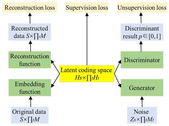
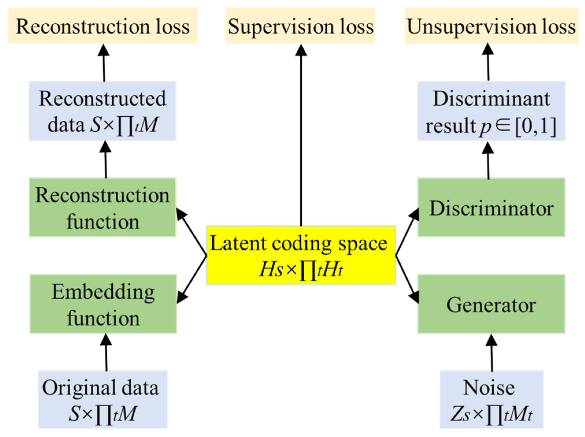
The TimeGAN model consists of four components: a generator, a discriminator, an embedding function, and a recovery function, as illustrated in Figure 1.

Figure 1. Diagram of the TimeGAN Model Architecture.

2.1. Embedding Function and Reconstruction Function

The proposal of the embedding function and reconstruction function is grounded in the fact that high-dimensional, complex temporal dynamics are often driven by lower-dimensional, simpler underlying factors of variation. Therefore, the embedding function and reconstruction function provide a low-dimensional latent space for the network to learn these key factors of variation.

The purpose of the embedding function is to reduce the dimensionality of the original time series, thereby enhancing the efficiency of model learning. The embedding function processes both static and temporal features through recursion. For static features, it projects them into a low-dimensional space; for temporal features, it explores the relationships between time points and projects them into the same low-dimensional space.

$$h_S=e_S(s)$$

(1)

$$h_t=e_m(h_S,h_{t-1},M_t)$$

(2)

Here, $e_S$ and $e_m$ represent the processing of static and temporal features by the embedding function, respectively. $h_S$ denotes the static features after dimensionality reduction by the embedding function, $h_t$ represents the temporal features at time t after dimensionality reduction, and $M_t$ represents the high-dimensional temporal features at time t.

The reconstruction function, on the other hand, is designed to reconstruct the low-dimensional vectors, after dimensionality reduction, back into high-dimensional vectors in the original space. The process is as follows:

$$\tilde{S}=r_S(h_S)$$

(3)

$${\tilde{M}}_t=r_M(h_t)$$

(4)

Here, $r_S$ and $r_M$ represent the processing of low-dimensional static and temporal features by the reconstruction function, respectively. $\tilde{S}$ denotes the reconstructed static features, and ${\tilde{M}}_t$ represents the reconstructed temporal features at time t.

2.2. Generator and Discriminator

The generator first randomly samples vectors from the vector spaces of static and temporal features, which follow known given distributions, and inputs them into a low-dimensional latent space. The process is as follows:

$${\stackrel{{\displaystyle ⌢}}{h}}_S=g_S(z_S)$$

(5)

$${\stackrel{⌢}{h}}_t=g_M({\stackrel{⌢}{h}}_S,{\stackrel{⌢}{h}}_{t-1},z_t)$$

(6)

Here, $g_S$ and $g_M$ are the generative networks for static and temporal features, respectively. $z_S$ and $z_t$ represent the sampling from the vector spaces of static and temporal features, respectively, while ${\stackrel{⌢}{h}}_S$ and ${\stackrel{⌢}{h}}_t$ denote the generated sets of static and temporal feature vectors, respectively.

The output results of the generator and those output by the embedding function are jointly encoded and then input into the discriminator. At this point, the discriminator will evaluate the authenticity by comparing the real data with the generated data. If the discriminator outputs 1, it indicates authenticity; if it outputs 0, it indicates falsity. The process is as follows:

$${\tilde{y}}_S=d_S({\tilde{h}}_S)$$

(7)

$${\tilde{y}}_t=d_M({\overleftarrow{u}}_t,{\overrightarrow{u}}_t)$$

(8)

Here, ${\tilde{y}}_S$ and ${\tilde{y}}_t$ represent the discrimination results for the static and temporal features of the input data, respectively. $d_S$ and $d_M$ denote the discrimination networks for static and temporal features, respectively. When utilizing a bidirectional recurrent network with a feedforward output layer, ${\overleftarrow{u}}_t$ and ${\overrightarrow{u}}_t$ represent the forward and backward hidden state sequences, respectively.

2.3. Training Loss

For the embedding function and reconstruction function, their objective should be to generate the low-dimensional latent space and reconstruct the high-dimensional original feature space as accurately as possible. Therefore, the first loss is introduced:

$$L_{e-r}=E_{S,M_{1:T\sim p}}[{‖S‖}_2+{\displaystyle \sum _t{‖M_t‖}_2}]$$

(9)

Here, the meanings of S and M are as previously described. Regarding the generator and discriminator in the model, there exists a classic game, and the second loss is introduced as follows:

$$L_{g-d}=E_{S,M_{1:T\sim p}}[\log y_s+{\displaystyle {\sum }_t\log y_t}]+E_{S,M_{1:T\sim \tilde{p}}}[\log (1-{\overline{y}}_s)+{\displaystyle {\sum }_t(1-\log {\overline{y}}_t})]$$

(10)

Here, $y_s$ and $y_t$ represent the discrimination results for the static and temporal features of the original data, respectively, while ${\overline{y}}_s$ and ${\overline{y}}_t$ denote the discrimination results for the static and temporal features of the generated data, respectively.

The introduction of $L_{g-d}$ enables the model to focus on describing the overall probability distribution of the time-series data, but it fails to learn the point-by-point conditional probability distribution. Therefore, a third loss is introduced to achieve this:

$$L_S=E_{S,M_{1:T\sim p}}[{{\displaystyle {\sum }_t‖h_t-g_M(h_S,h_{t-1},z_t)‖}}_2]$$

(11)

The training losses of TimeGAN fall into three categories: The embedding reconstruction loss serves as the foundation, constraining the embedding and reconstruction functions to ensure that the latent space effectively carries core information and avoids information loss, thus acting as a prerequisite for subsequent training. The adversarial loss is the core of the generative adversarial network, governing the adversarial game between the generator and discriminator to make the generated data align with the overall probability distribution of the original data and restore macroscopic characteristic patterns. The supervised loss is a newly added key loss that compensates for the limitations of the adversarial loss by constraining the generator to ensure that the generated time-series data matches the real data in terms of fine-grained correlations at time points, such as the continuous variation patterns of photovoltaic power output under different time instants and weather conditions, making the generated data more consistent with the actual time-series variations in photovoltaic power output.

3. Clustering Analysis of Photovoltaic Weather Features Based on the K-Means Method

After the TimeGAN model generates data, a large amount of generated data can be utilized to screen for weather factors that exhibit strong correlations with PV power output. To further uncover the underlying association patterns between PV power output and weather conditions, this paper employs a clustering algorithm to address the complex relationships among multiple variables. By performing clustering after data dimensionality reduction, all factors within the PV weather system are categorized into their respective groups.

3.1. Weather Factor Screening

The weather dataset generated by the TimeGAN model encompasses various weather factors, including temperature, humidity, rainfall, wind speed, and solar irradiance. It is necessary to select meteorological variables that exhibit significant statistical correlations with PV power output and load power while ensuring they are non-redundant. By analyzing the Pearson correlation coefficient of historical data, we can quantitatively evaluate the strength of the associations between each meteorological factor and PV power output, as well as load. The calculation formula is as follows:

$$\rho ={\displaystyle \frac{\mathrm{cov}(X,Y)}{{\sigma }_X{\sigma }_Y}}$$

(12)

Here, cov(X,Y) and σ_X, σ_Y represent the covariance and standard deviations between variables X and Y, respectively, while p denotes the Pearson correlation coefficient of X and Y. Relevant theory indicates that when |p| > 0.5, the two variables are considered to have a strong correlation.

3.2. K-Means Algorithm

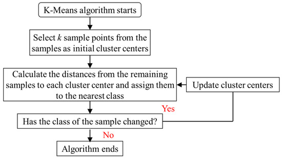
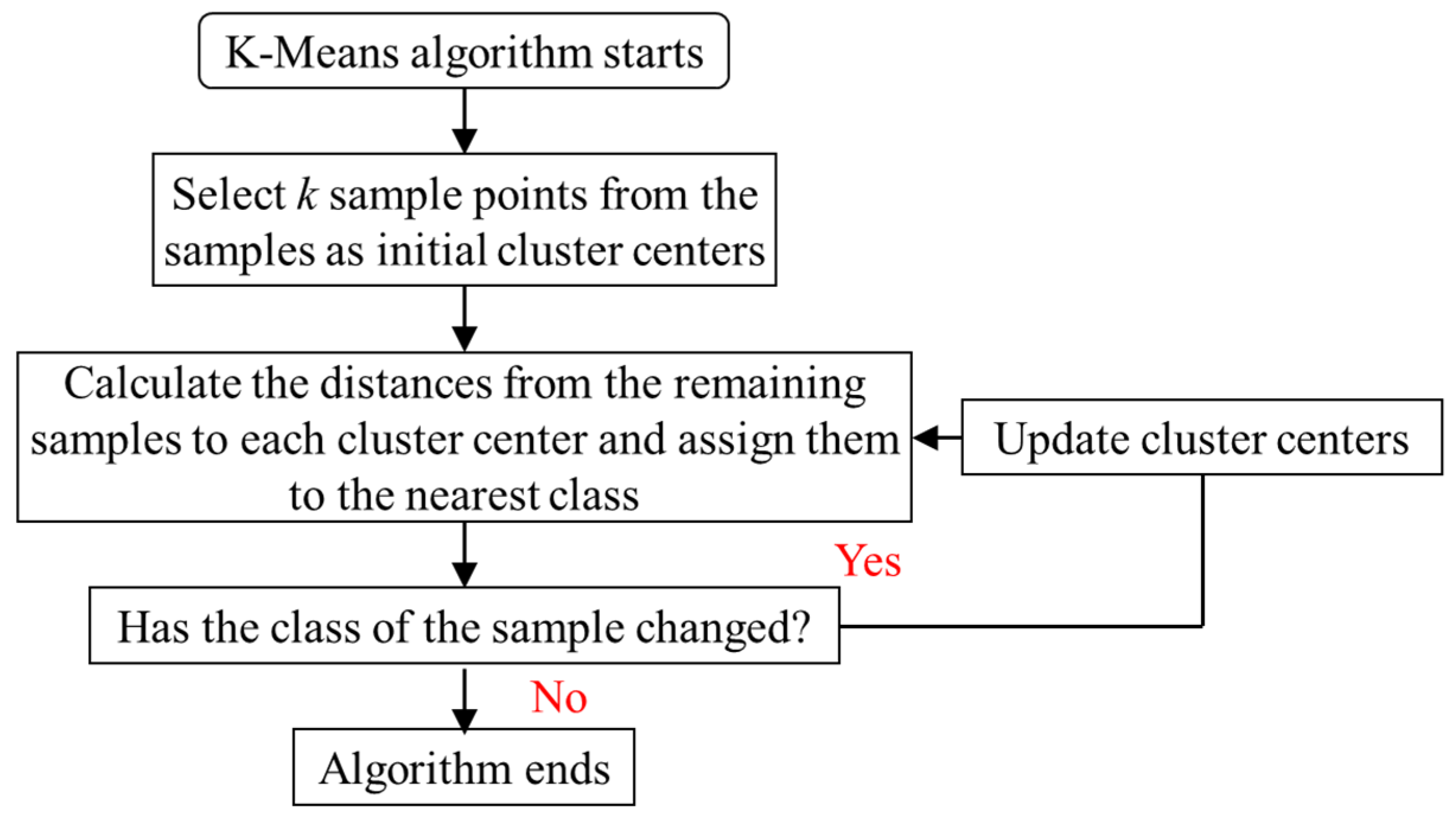
The k-means algorithm is an unsupervised learning clustering algorithm that can partition data into a finite number of categories. Its objective is as follows: For a dataset $X=\left\{x_1,x_2,\dots ,x_n\right\}$ (where $x_i$ is a j-dimensional vector, $x_i=\left\{x_{i1},x_{i2},\dots ,x_{ij}\right\}$), k-means divides X into k clusters such that the data points within each cluster are closest to the cluster centroid of that cluster. The flowchart of the algorithm is shown in Figure 2.

Figure 2. The flowchart of the k-means algorithm.

In the clustering process illustrated in Figure 2, the data input encompasses time series of PV power output generated by the TimeGAN model, along with corresponding meteorological factor data, including temperature, humidity, wind speed, and solar radiation. These data, after undergoing preprocessing to ensure quality, are utilized for clustering analysis. The output of the clustering process is the result of dividing these data into K clusters, with each cluster representing a pattern characterized by similar PV power output and meteorological features. Additionally, the output includes the centroids of each cluster, which serve as representatives of their respective clusters, revealing the typical characteristics of PV power output and their associated meteorological patterns under different scenarios. In this paper, the k-means algorithm adopts the initialization method of the k-means++ algorithm during initialization. Compared to the standard k-means algorithm, this approach increases the probability of selecting points that are far apart from each other as the initial cluster centroids. This modification effectively avoids the slow convergence issue often encountered with the k-means algorithm.

In the k-means algorithm, the number of clusters (K) needs to be manually determined. The elbow method can be employed for this selection. The elbow method is based on the sum of squared errors (SSE), which is defined as

$$SSE={\displaystyle \sum _{i=1}^k{{\displaystyle \sum _{p\in C_i}\left|q-m_i\right|}}^2}$$

(13)

Here, k represents the number of clusters, C_i denotes the i-th cluster, q is a sample point within C_i, and m_i signifies the cluster centroid of the i-th cluster.

4. Mathematical Model for Secure and Economical Operation Control of Power Systems

4.1. Objective Function

This paper formulates optimal scheduling objectives from both security and economic perspectives. On the security front, the objective is to minimize voltage fluctuations, with the relevant expression as follows:

$$ob{j}_1={\lambda }_u{\displaystyle \sum _{t=1}^T{\displaystyle \sum _{i=1}^I\left|\frac{U_{i,t}-U_{i,N}}{U_{i,N}}\right|}}$$

(14)

Here, T represents the total scheduling time periods, and I denotes the total number of nodes. $U_{i,t}$ indicates the voltage magnitude at node i during time period t, while $U_{i,N}$ represents the standard voltage value at node i. ${\lambda }_u$ denotes the penalty coefficient for voltage fluctuations.

On the economic front, this paper aims to minimize load shedding, as shown in (15).

$$ob{j}_2={\lambda }_L{\displaystyle \sum _{t=1}^T{\displaystyle \sum _{i=1}^I\mathrm{\Delta }{P}_{i,t}}}$$

(15)

Here, ${\lambda }_L$ represents the penalty cost for load shedding, and $\mathrm{\Delta }{P}_{i,t}$ denotes the amount of load shed at node i at time t.

By combining the aforementioned two sub-objective functions, the mathematical model for the final scheduling objective is presented as follows:

$$obj=ob{j}_1+ob{j}_2$$

(16)

The strategy proposed in this paper is essentially a robust stochastic optimization framework constructed based on multi-scenario generation technology: It generates a set of typical scenarios with probabilistic distribution characteristics through historical data clustering and employs scenario weight allocation to depict the fluctuation range of uncertain parameters. This approach implicitly considers the robust coverage of extreme scenarios and the economic balance of regular scenarios within the optimization model. Although it does not explicitly incorporate chance constraints, minimax structures, or two-stage recourse mechanisms, the construction process of the scenario set integrates the concept of statistical robustness. The convergence of the objective function value as the number of scenarios increases indirectly validates the effective modeling of uncertainty. Therefore, the formulation of the robust stochastic auxiliary model aims to emphasize the strategic coupling characteristics of this method between determinism and stochasticity.

4.2. Constraints

(1)

Power Flow Constraints

$$P_{ij,t}=-P_{j,t}+{\displaystyle \sum _{k\in ch(j)}{P}_{jk,t}}$$

(17)

$$Q_{ij,t}=-Q_{j,t}+{\displaystyle \sum _{k\in ch(j)}{Q}_{jk,t}}$$

(18)

$$U_{i,t}-U_{j,t}=r_{ij}{P}_{ij,t}+x_{ij}{Q}_{ij,t}$$

(19)

$$U_{\min }\le U_{i,t}\le U_{\max }$$

(20)

$$P_{l,\min }\le P_{ij,t}\le P_{l,\max }$$

(21)

where $P_{ij,t}$ and $Q_{ij,t}$ represent the active power and reactive power transmitted between nodes i and j at time t, respectively; $P_{j,t}$ and $Q_{j,t}$ denote the active and reactive power injections at node j at time t, respectively; $U_{i,t}$ and $U_{j,t}$ are the voltage magnitudes at nodes i and j at time t, respectively; $r_{ij}$ and $x_{ij}$ are the line resistance and reactance between nodes i and j, respectively; (20) represents the voltage fluctuation range at nodes; (21) specifies the upper and lower limits for the active power transmitted through the line.

(2)

OLTC Voltage Regulation Model

The OLTC voltage regulation model in the distribution network is represented by Equations (22)–(27). It primarily alters the transformer turns ratio by adjusting the tap positions.

$$U_{H,t}=B_{oltc,t}·U_{L,t}$$

(22)

$$B_{oltc,t}=B_{oltc,\min }+\mathrm{\Delta }B·b_t$$

(23)

$${\delta }_{up,t}+{\delta }_{dn,t}\le 1$$

(24)

$$b_t-b_{t-1}\ge {\delta }_{up,t}-{\delta }_{dn,t}·SR$$

(25)

$$b_t-b_{t-1}\le {\delta }_{up,t}·SR-{\delta }_{dn,t}$$

(26)

$${\displaystyle \sum ({\delta }_{up,t}+{\delta }_{dn,t})}\le N_{\max }^{oltc}$$

(27)

Here, $U_{H,t}$ and $U_{L,t}$ represent the voltages on the high-voltage and low-voltage sides of the transformer, respectively; $B_{oltc,t}$ is the transformer turns ratio at time t; Equation (23) indicates the adjustable upper and lower limits of the turns ratio; $\mathrm{\Delta }B$ denotes the unit adjustment step size, and $b_t$ is the tap position at time t; Equations (24)–(27) represent the daily usage limit of the OLTC; ${\delta }_{up,t}$ and ${\delta }_{dn,t}$ are the state variables for tap position changes; when ${\delta }_{up,t}$ is 1, it indicates an upward tap adjustment; when ${\delta }_{dn,t}$ is 1, it indicates a downward tap adjustment; SR represents the maximum reachable tap position; $N_{\max }^{oltc}$ denotes the maximum number of daily operations.

(3)

Reactive Power Compensation Device Model

To simplify calculations, this paper employs a continuous modeling approach for discrete reactor banks and capacitor banks, as shown in Equation (28):

$$RP{C}_{\min }\le RP{C}_t\le RP{C}_{\max }$$

(28)

where $RP{C}_t$ represents the reactive power output at time t, with the reactive power variation range extending from negative to positive values.

(4)

Energy Storage System Model

$$ES{S}^t=ES{S}^{t-1}+(P_c^{t-1}{\eta }_c-{\displaystyle \frac{P_d^{t-1}}{{\eta }_d}})\mathrm{\Delta }t$$

(29)

$$ES{S}_{\min }\le ES{S}^t\le ES{S}_{\max }$$

(30)

$$u_{d,t}+u_{c,t}\le 1$$

(31)

$$0\le P_c^t\le u_{c,t}{P}_{c,\max }$$

(32)

$$0\le P_d^t\le u_{d,t}{P}_{d,\max }$$

(33)

Here, $ES{S}^t$ represents the energy level of the energy storage battery at time t; ${\eta }_c$ and ${\eta }_d$ denote the charging and discharging efficiencies, respectively; $u_{c,t}$ and $u_{d,t}$ indicate the charging and discharging states at time t, respectively; $P_c^t$ and $P_d^t$ represent the charging and discharging powers at time t, respectively, while $P_{c,\max }$ and $P_{d,\max }$ denote the extreme values of the charging and discharging powers.

(5)

Demand Response Model

This paper employs a price-based demand response model, establishing time-of-use electricity pricing and utilizing a dynamic pricing mechanism to guide users in adjusting their electricity consumption behavior. Additionally, an elasticity coefficient matrix, incorporating elasticity impact weights, is introduced. The expression is as follows:

$$L_{ii,ij}=\left\{\begin{array}{c}{L}_{ii}={\displaystyle \frac{\mathrm{\Delta }{P}_{load,i}·C_{e,i}}{P_{load,i}·\mathrm{\Delta }{C}_{e,i}}}\\ L_{ij}={\displaystyle \frac{\mathrm{\Delta }{P}_{load,i}·C_{e,j}}{P_{load,i}·\mathrm{\Delta }{C}_{e,j}}}\end{array}\right.$$

(34)

$${\beta }_{ii,ij}=\left\{\begin{array}{c}{\beta }_{ii}={\displaystyle \frac{\mathrm{\Delta }{P}_{ii}}{\mathrm{\Delta }{P}_i}}\\ {\beta }_{ij}={\displaystyle \frac{\mathrm{\Delta }{P}_{ij}}{\mathrm{\Delta }{P}_i}}\end{array}\right.$$

(35)

$$L_{ii,ij}^{\mathrm{\Delta }}=\left[\begin{array}{cccc}{\beta }_{11}{L}_{11}& {\beta }_{12}{L}_{12}& \dots & {\beta }_{1n}{L}_{1n}\\ {\beta }_{21}{L}_{21}& {\beta }_{22}{L}_{22}& \dots & {\beta }_{2n}{L}_{2n}\\ ⋮& ⋮& \dots & ⋮\\ {\beta }_{n1}{L}_{n1}& {\beta }_{n2}{L}_{n2}& \dots & {\beta }_{nn}{L}_{nn}\end{array}\right]$$

(36)

where $L_{ii,ij}^{\mathrm{\Delta }}$ represents the elasticity matrix under the time-of-use pricing scheme; $P_{load,i}$ denotes the load quantity prior to demand response; $\mathrm{\Delta }{P}_{load,i}$ indicates the load reduction resulting from demand response; $C_{e,i}$ represents the electricity price before demand response; $\mathrm{\Delta }{C}_{e,i}$ signifies the price differential before and after demand response; $\mathrm{\Delta }{P}_{ij}$ denotes the load variation between moment j and moment i; $\mathrm{\Delta }{P}_i$ represents the overall load change at moment i. Taking load quantity and time-of-use electricity pricing as the research subjects, this study analyzes their relationship using elasticity theory, with a cycle set at 24 h. The expression for the load response model is as follows:

$$P_L=P_{load,i}(1+L_{ii,ij}^{\mathrm{\Delta }}{\displaystyle \frac{\mathrm{\Delta }{C}_{e,i}}{C_{e,i}}}+{\displaystyle \sum _{i=1,j\ne i}^{24}{L}_{ii,ij}^{\mathrm{\Delta }}\frac{\mathrm{\Delta }{C}_{e,i}}{C_{e,i}}})$$

(37)

5. Solution Strategy Based on Improved Harris’s Hawks Optimization

The IHHO algorithm draws its design inspiration from the cooperative behavior and surprise-attack hunting style of Harris’s hawks during prey capture. The optimization process of the algorithm comprises three stages: exploration, transition between exploration and exploitation, and exploitation.

5.1. Algorithmic Strategy

The IHHO imitates the cooperative behavior and surprise-attack hunting style of Harris’s hawks during their predation on prey. The positions of Harris’s hawks are regarded as candidate solutions, while the position of the prey represents the best candidate solution in each iteration.

(1)

Exploration Phase

In the early stage, Harris’s hawks remain in a waiting state and employ two strategies with equal probability for searching for prey. The expression is as follows:

$$x_z^{t+1}=\left\{\begin{array}{c}{x}_{rand}^t-g_1·\left|x_{rand}^t-2g_2·x_z^t\right|,\hspace{1em}\hspace{1em}\hspace{1em}q\ge 0.5\\ (x_{prey}^t-x_m^t)-g_3·(L_b+g_4·(U_b-L_b)),\hspace{1em}\hspace{1em}\hspace{1em}q\ge 0.5\end{array}\right.$$

(38)

Here, $x_z^t$ represents the coordinates of the z-th individual in the t-th update iteration; $x_{rand}^t$ represents the coordinates of an individual randomly selected from the population during the t-th update iteration, q and $g_o(o=1,2,3,4)$ are random numbers within the range [0, 1]; $x_{prey}^t$ represents the coordinates of the optimal individual in the population during the t-th update iteration; $x_m^t$ represents the average coordinates of the population during the t-th iteration, with the expression given by

$$x_m^t={\displaystyle \frac{{\displaystyle \sum _{z=1}^N{x}_z^t}}{N}}$$

(39)

where N represents the population size.

(2)

Exploration-Exploitation Transition Phase

IHHO analyzes the prey’s escape energy to accomplish the transition from the exploration phase to the exploitation phase, with the expression given by

$$E=2E_0(1-k/K)$$

(40)

where $E_0$ represents the initial escape energy of the prey; k and K represent the current iteration number and the maximum iteration number, respectively.

When $\left|E\right|>1$, Harris’s hawks search different areas to locate the prey, which is the exploration phase; when $\left|E\right|<1$, the population explores for the optimal solution within the range of the current solution, which is the exploitation phase.

(3)

Exploitation Phase

Based on the prey’s escape maneuvers and Harris’s hawks’ capture strategies, Harris’s hawks employ four methods to mimic the capture behavior.

Method 1: Soft Encirclement

When $0.5\le \left|E\right|<1$ and $r\ge 0.5$, the prey has sufficient energy to escape, the energy of the prey is gradually depleted. The coordinate update expression is

$$x_z^{t+1}=x_{prey}^t-x_z^t+E·\left|J·x_{prey}^t-x_z^t\right|$$

(41)

Here, J represents the jumping intensity of the prey during its escape process, $J\in [0,2]$ and its expression is given by

$$J=2·(1-r_5)$$

(42)

Method 2: Hard Encirclement

When $\left|E\right|<0.5$ and $r\ge 0.5$, Harris’s hawks launch a rapid assault as the prey’s energy is exhausted. The coordinate update expression is

$$x_z^{t+1}=x_{prey}^t-E·\left|x_{prey}^t-x_z^t\right|$$

(43)

Method 3: Progressive Rapid Dive with Soft Encirclement

When $0.5\le \left|E\right|<1$ and $r<0.5$, Harris’s hawks swiftly launch an assault to capture the prey. While diving towards the prey, Harris’s hawks anticipate their next move, with the expression given by

$$Y=x_{prey}^t-E·\left|J·x_{prey}^t-x_z^t\right|$$

(44)

While diving towards the prey, the optimal diving approach for the current action is evaluated and compared with the previous one. If the Harris’s hawk detects deceptive behavior from the prey, indicating that the candidate solution is not worth pursuing, it will alter its diving approach for the next attempt, with the expression given by

$$Z=Y+S·H(D)$$

(45)

Here, D represents the dimension of the optimization problem; S denotes a D-dimensional random vector, $S\in [0,1]$; $H(D)$ represents another D-dimensional random vector.

The coordinate update expression is given by

$$x_z^{t+1}=\left\{\begin{array}{c}Y,f(Y)<f(x_z^t)\\ Z,f(Z)<f(x_z^t)\end{array}\right.$$

(46)

where f(⋅) represents the value of the objective function.

Method 4: Progressive Rapid Dive with Hard Encirclement

When $\left|E\right|<0.5$ and $r<0.5$, Harris’s hawks swiftly launch an assault to capture the prey. While diving towards the prey, Harris’s hawks anticipate their next move, with the expression given by

$$Y=x_{prey}^t-E·\left|J·x_{prey}^t-x_m^t\right|$$

(47)

5.2. Algorithm Improvement

Improvement 1: Integration of ICMIC Chaotic Mapping

In the initial stage of IHHO, the population is randomly generated, leading to uneven distribution of the population and consequently reducing the algorithm’s global search capability. To enhance the uniformity and rationality of population initialization, chaotic mapping is employed to initialize the population, thereby improving the traversal of the population at the start of the algorithm. The ICMIC mapping is introduced to generate chaotic sequences for initializing the population, thereby enhancing the algorithm’s global search capability and enabling it to more effectively locate the global optimum. The expression for the ICMIC mapping is as follows:

$$\left\{\begin{array}{c}{x}_{n+1}=\sin {\displaystyle \frac{a}{x_n}},\hspace{1em}\hspace{1em}a\in (0,\infty )\\ -1<x_n<1\end{array}\right.$$

(48)

Here, a represents a control parameter, which is set to 100 in this paper.

Improvement 2: Levy Flight Function

Levy(D) denotes a D-dimensional random vector generated by Levy flight. The Levy distribution is continuously stable for non-negative random variables. Levy(x) represents the Levy flight function, with its expression given by

$$\left\{\begin{array}{c}Levy(x)=0.01\times {\displaystyle \frac{\mu ·\sigma }{{\left|\upsilon \right|}^{1/\beta }}}\\ \sigma ={\left[{\displaystyle \frac{\mathrm{\Gamma }(1+\beta )\times \sin \frac{\pi \beta }{2}}{\mathrm{\Gamma }(\frac{1+\beta }{2})\times \beta \times 2^{(\frac{\beta -1}{2})}}}\right]}^{1/\beta }\\ \mathrm{\Gamma }(y)=(y-1)!\end{array}\right.$$

(49)

where $\mu$ and $\upsilon$ represent random numbers within the range of [0, 1]; $\beta$ is a constant, which is set to 1.5 in this paper. IHHO conducts local exploitation through four strategies and maintains a good balance between exploring new solutions and exploiting current solutions by dynamically adjusting its hunting strategies.

6. Case Study

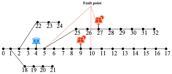
To illustrate the effectiveness of the method proposed in this paper, a modified IEEE-33-node test system is employed for analysis. The topological structure of this test system is shown in Figure 3 below. Specifically, two distributed photovoltaic power generation systems are installed at nodes 9 and 27, respectively. An energy storage system is installed at node 4. Faults occur at nodes 5, 10, and 27, causing power fluctuations at these nodes. TimeGAN adopts a four-stage cascaded architecture consisting of an embedder, a generator, a discriminator, and a reconstructer, which is tailored for learning both static and dynamic features of photovoltaic power output temporal data. The network structures and functions of each module are as follows: The embedder employs two layers of long short-term memory (LSTM) networks and one fully connected (FC) layer to map high-dimensional photovoltaic temporal data (power output + meteorological factors) into a low-dimensional latent space, extracting core features. The generator utilizes two layers of LSTM with dropout and one FC layer to generate photovoltaic power output temporal data that aligns with the real distribution from random noise combined with latent space features. The discriminator employs two layers of bidirectional LSTM networks and one FC layer (with a sigmoid activation function in the output layer) to distinguish between real photovoltaic data and generated data while also evaluating the “authenticity” and “temporal consistency” of the temporal data. The reconstructer uses two layers of LSTM networks and one FC layer to reconstruct the latent space features back into photovoltaic data of the original dimension, verifying the effectiveness of feature representation. The dimension of the LSTM hidden layers is set to 128, and the sequence input dimension is 16. Regarding the dropout layer, a dropout layer with a dropout rate of 0.2 is incorporated into the generator to prevent the model from overfitting to local fluctuation characteristics of photovoltaic power output. The hardware setup includes an NVIDIA RTX 3090 GPU (with 24 GB of memory), an Intel i9-12900K CPU made in USA, and 64 GB of RAM. The software environment consists of Python 3.8, PyTorch 1.12.0 (as the deep learning framework), Pandas/Numpy (for data processing), and Matplotlib (for result visualization). Parallel acceleration is achieved through GPU batch processing computation, with each training round taking approximately 0.8 s and the total training duration being around 30 min. The distributed PV unit employs N-type monocrystalline silicon modules, with a rated power of 550 W per module, a total installed capacity of 500 kWh, and is equipped with a 500 kVA inverter boasting an efficiency of ≥98.5%. It features overvoltage protection and low-voltage ride-through capability. The energy storage system utilizes lithium iron phosphate batteries, with a total capacity of 224 kWh/100 kW and a charging/discharging efficiency of ≥95%. The OLTC provides three-phase regulation, featuring 17 taps, a single-tap voltage regulation of 0.025 p.u., and a voltage regulation range of 0.8 to 1.2 p.u. The photovoltaic data is sourced from the U.S. National Renewable Energy Laboratory dataset [28], while the accompanying meteorological dataset, including temperature, humidity, solar radiation, and wind speed, is obtained from the NASA POWER meteorological database [29].

Figure 3. Topological structure of the test system.

The typical PV scenarios generated in this paper are shown in Figure 4 and Figure 5 below.

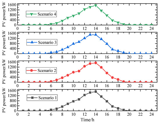
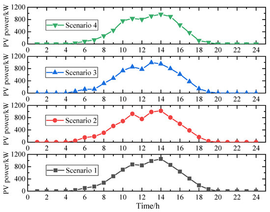
Figure 4. PV power at node 9.

Figure 5. PV power at node 27.

By observing the figure above, it can be found that the advantage of generating typical PV output scenarios using the method proposed in this paper lies in its ability to integrate historical operational data and utilize the TimeGAN model to capture both static and temporal features of PV output, thereby generating high-quality, diverse time-series data scenarios. This approach not only considers the historical variation patterns of PV output but also learns point-wise conditional probability distributions through the introduction of supervised loss training, thus more comprehensively reflecting the complexity and diversity of PV output. Furthermore, by incorporating the k-means clustering algorithm for cluster analysis of PV weather characteristics, it further reveals potential correlation patterns between PV output and weather factors, making the generated typical scenarios closer to actual operational conditions and enhancing their representativeness and practicality. The method’s ability to accurately reflect the volatility and uncertainty of PV output mainly stems from the TimeGAN model’s refined capability to capture both static and temporal features of time-series data. By introducing embedding and reconstruction functions, TimeGAN maps high-dimensional complex temporal dynamics into a low-dimensional latent space, enabling the model to learn key variation factors more efficiently. Meanwhile, the game process between the generator and discriminator ensures the quality and diversity of the generated data, allowing the generated scenarios to fully reflect the volatility and uncertainty of PV output. Additionally, by screening weather factors strongly correlated with PV output through cluster analysis and considering their impact on PV output, the portrayal of PV volatility and uncertainty in the generated scenarios is further enhanced.

Building upon the existing visual representation of photovoltaic scenarios, the following evaluation metrics have been introduced for quantitative analysis. The Kullback–Leibler (KL) divergence measures the discrepancy in probability distributions between the generated data and historical data, with smaller values indicating closer distributions. The calculated KL divergence between the generated data and historical data is 0.037, significantly lower than the 0.121 observed with the traditional GAN model. The Wasserstein distance reflects the geometric distance between two distributions, and on the test set, the Wasserstein distance between the generated data and real data is 0.082, representing a 56% reduction compared to the LSTM model. The maximum mean discrepancy (MMD), which is based on kernel methods for distribution similarity testing, yields an MMD value of 0.045 using a Gaussian kernel function, validating the consistency of the distributions. Under a predefined 5% extreme scenario threshold, the generated data successfully captures 98.7% of the power fluctuations corresponding to historical extreme weather events, representing a 21% improvement over the Monte Carlo simulation method. The data characteristic values under different prediction models are presented in Table 1 below.

Table 1. Data characteristic values under different prediction models.

Evaluation Metrics	Historical Data	TimeGAN	Traditional GAN	LSTM
Average Power/kW	125.3	124.8	121.6	123.7
Maximum Power (kW)	312.5	310.1	305.2	308.4
Minimum Power (kW)	12.7	13.2	10.5	15.1
Standard Deviation Peak-to-Valley	87.4	86.9	82.1	84.3
Difference Ratio	0.92	0.91	0.89	0.90
Extreme Scenario Coverage Rate	-	98.7%	76.3%	82.1%

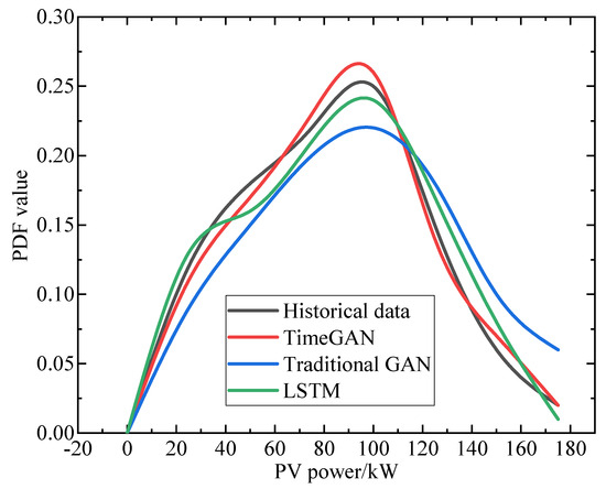
Figure 6 presents the comparative data of probability density functions (PDFs) of different methods.

Figure 6. PDFs of different methods.

The error in PDF values between TimeGAN and historical data within the core power generation range of 50–125 kW is ≤5%, with a peak position deviation of only 1 kW. The peak value in the historical data is 102 kW, while the peak value in the generated data is 101 kW. The traditional GAN overestimates the PDF values by 33% in the range above 125 kW, leading to overfitting in extreme scenarios. The LSTM underestimates by 17% in the low power range of 0–25 kW, failing to accurately capture residual power generation at night.

The Pearson correlation coefficients for each variable are presented in Table 2 below.

Table 2. Pearson correlation coefficients for each variable.

Variable	PV Power	Solar Radiation	Temperature	Humidity	Wind Speed
PV Power	1.000	0.982	0.876	−0.654	−0.312
Solar Radiation	0.982	1.000	0.891	−0.687	−0.298
Temperature	0.876	0.891	1.000	−0.432	−0.105
Humidity	−0.654	−0.687	−0.432	1.000	0.087
Wind Speed	−0.312	−0.298	−0.105	0.087	1.000

PV power exhibits a strong positive correlation with solar radiation (r = 0.982) and temperature (r = 0.876), while showing a significant negative correlation with humidity (r = −0.654), aligning with physical principles: increased cloud cover reduces radiation and raises humidity. Wind speed demonstrates a weak correlation with photovoltaic power (r = −0.312) and is excluded from subsequent cluster analysis to minimize noise. Solar radiation serves as the direct driving factor for photovoltaic power generation; hence, its correlation coefficient approaches 1. Temperature indirectly affects output by influencing photovoltaic cell efficiency, albeit with a lag effect, resulting in a slightly lower correlation coefficient. Elevated humidity thickens cloud cover, reducing radiation and exhibiting a negative correlation. Wind speed has a limited impact on local microclimates, resulting in an insignificant correlation.

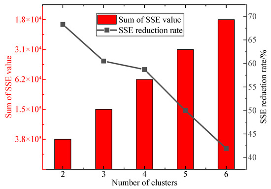
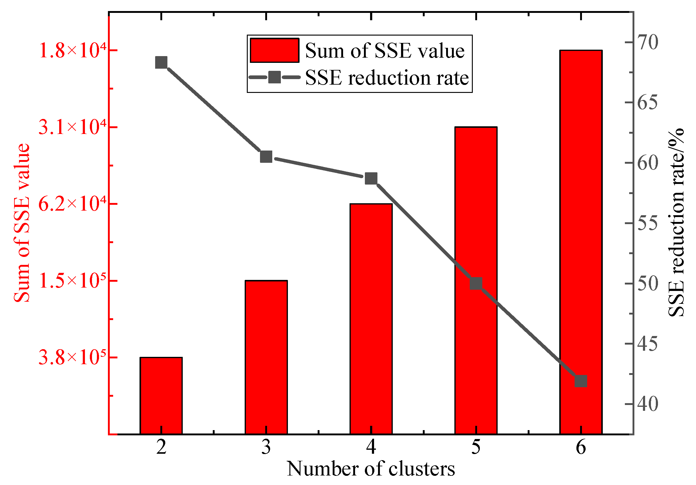
The elbow method was employed to determine the optimal number of clusters, as illustrated in Figure 7 below.

Figure 7. Analysis of optimal cluster number.

When k = 4, the SSE reduction rate drops below 60% for the first time, and the rate of decline significantly slows down when k = 5, which aligns with the “elbow” characteristic. Therefore, k = 4 is selected. For k values ranging from 1 to 3, the within-cluster variance is relatively large, indicating underfitting of the model. When k = 4, the data is reasonably divided into four types of scenarios: “high radiation on sunny days,” “moderate radiation on cloudy days,” “low radiation on overcast days,” and “no radiation at night.” When k > 4, excessive subdivision leads to a decrease in inter-cluster differences, such as distinguishing between “thin cloud” and “thick cloud” scenarios, but the resolution of meteorological data is insufficient.

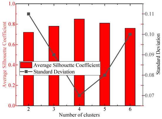
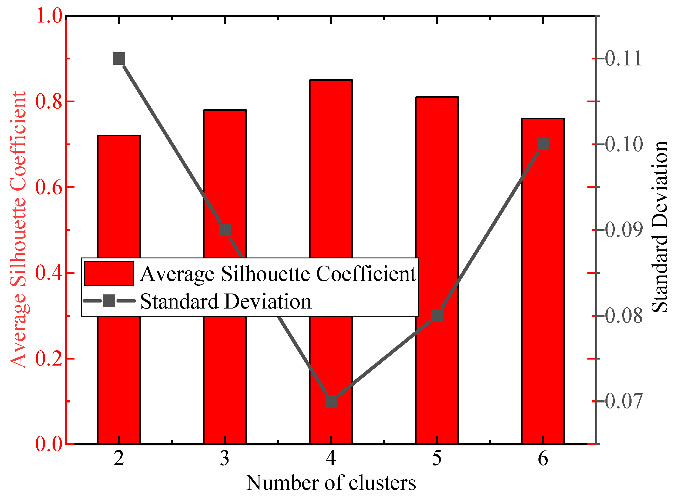
Figure 8 displays the Silhouette Coefficients for different numbers of clusters to validate the clustering quality.

Figure 8. Silhouette coefficients for different numbers of clusters.

When k = 4, the silhouette coefficient reaches its highest value (0.85), indicating tight clustering within each cluster and good separation between clusters. When k = 5, the coefficient decreases because over-segmentation leads to blurred boundaries for some clusters. When the silhouette coefficient approaches 1, it means that the distance between a sample and other samples within the same cluster is close, while the distance to samples in different clusters is far. For k = 4, the meteorological characteristics of the four types of scenarios differ significantly (e.g., solar radiation exceeds 800 W/m² on sunny days and is below 300 W/m² on overcast days), resulting in high separation. When k = 5, the newly added “local short-term shading” scenario overlaps with the “cloudy” scenario, causing the silhouette coefficient to decrease.

In addition to the SC, two other metrics have been selected as evaluation indicators. Specifically, the Calinski–Harabasz Index (CHI) reflects the ratio of inter-cluster variance to intra-cluster variance, with a higher ratio indicating a more reasonable clustering partition. The Davies–Bouldin Index (DBI) measures the average similarity between clusters, with a lower value indicating more significant differences between clusters and better non-overlapping properties. In the photovoltaic-meteorological fused feature dataset, artificial outliers were introduced at proportions of 5%, 10%, 15%, and 20%, while keeping the number of clusters k constant at 4. Clustering was repeated 10 times, and the mean and standard deviation of the evaluation metrics were calculated for each outlier proportion (Table 3).

Table 3. Robustness analysis of clustering.

Outlier Proportion	Mean SC ± Standard Deviation	Mean CHI ± Standard Deviation	Mean DBI ± Standard Deviation
0%	0.85 ± 0.012	1286.3 ± 45.2	0.21 ± 0.015
5%	0.83 ± 0.015	1215.7 ± 52.6	0.23 ± 0.018
10%	0.80 ± 0.021	1102.4 ± 68.9	0.27 ± 0.022
15%	0.72 ± 0.035	958.6 ± 89.3	0.35 ± 0.030
20%	0.61 ± 0.042	789.2 ± 105.7	0.48 ± 0.038

When the outlier proportion is ≤10%, the mean SC decreases by only 0.05, the mean CHI decreases by ≤14.3%, and the mean DBI increases by ≤28.6%. Moreover, the standard deviations of all metrics are relatively small (≤0.022), indicating that the clustering algorithm exhibits strong resistance to interference from low-proportion outliers. When the outlier proportion exceeds 15%, the metrics show significant deterioration due to the high proportion of outliers disrupting the inherent distribution patterns of PV-meteorological features. In practical engineering, the proportion of outliers in PV and meteorological monitoring data is typically ≤8% (after cleaning using the 3σ criterion). Therefore, the clustering method proposed in this paper demonstrates good robustness against outliers in practical applications.

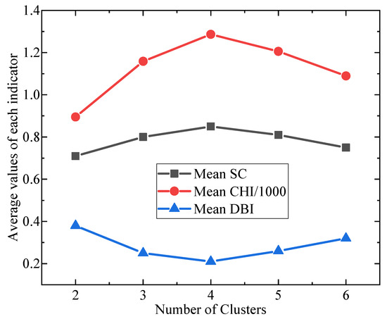
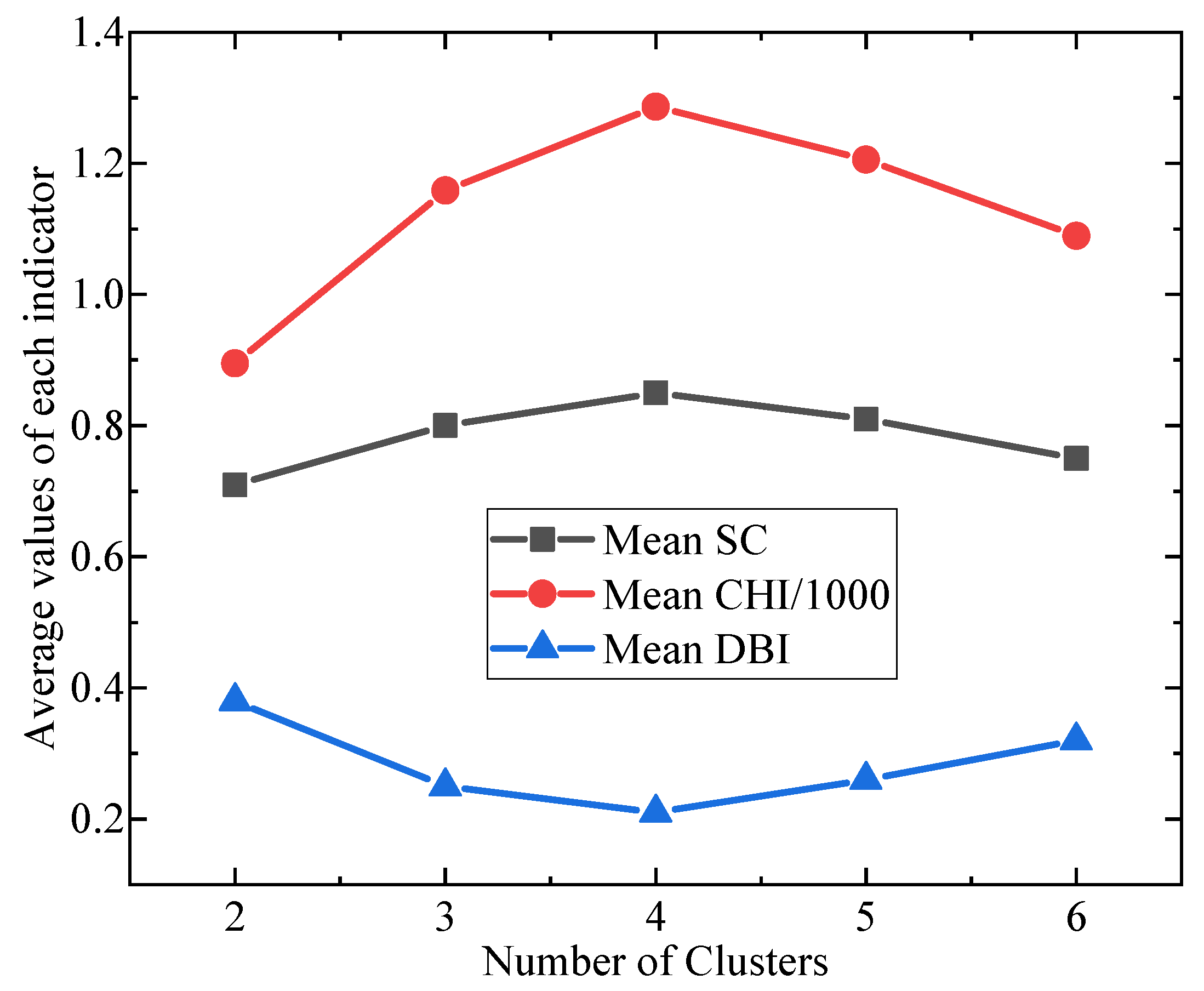
Keeping the PV-meteorological fused feature data unchanged, clustering was performed with the number of clusters k set to 2, 3, 4, 5, and 6, respectively. Clustering was repeated 10 times for each k value, and the mean values of the SC, CHI, and DBI were calculated, as shown in Figure 9.

Figure 9. Sensitivity analysis on the number of clusters.

SC exhibits an initial increase followed by a decrease as k increases, reaching its peak (0.85) at k = 4. When k < 4, the rise in SC is attributed to the enhanced similarity of samples within clusters due to an increased number of clusters. When k > 4, the decline in SC results from over-clustering, which blurs the boundaries between clusters and leads to the division of some similar samples into different clusters. CHI follows a similar trend to SC, reaching its maximum value (1286.3) at k = 4. When k > 4, the decrease in CHI is because the reduction in intra-cluster variance is less significant than the reduction in inter-cluster variance, thereby reducing the rationality of the clustering partition. DBI shows an initial decrease followed by an increase as k increases, reaching its minimum value (0.21) at k = 4. When k > 4, the rise in DBI is due to over-clustering, which increases the similarity between clusters and reduces the effectiveness of the clustering partition.

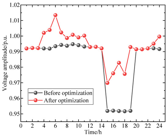
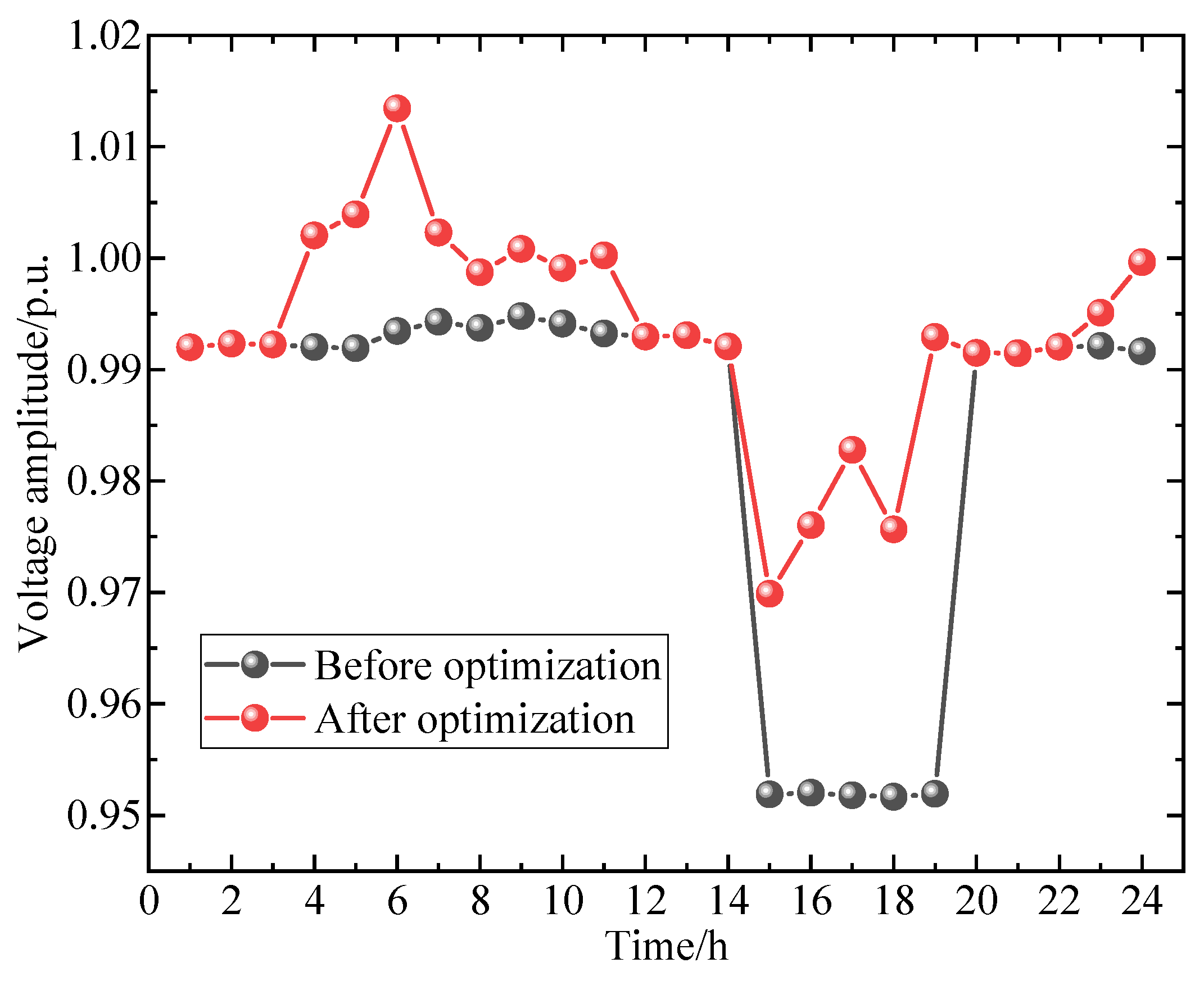
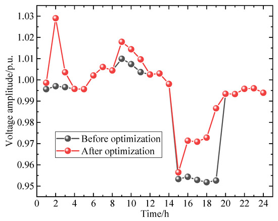
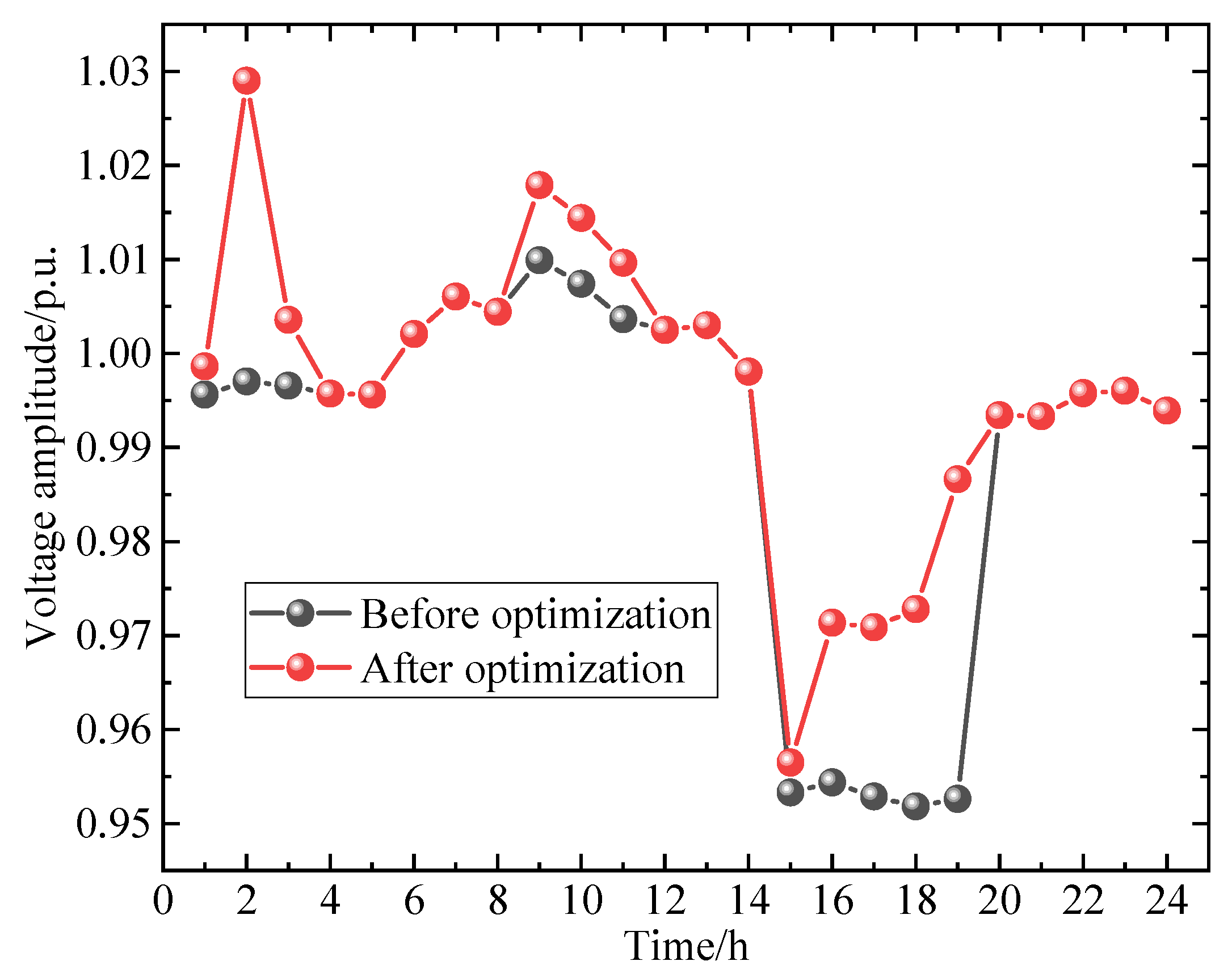
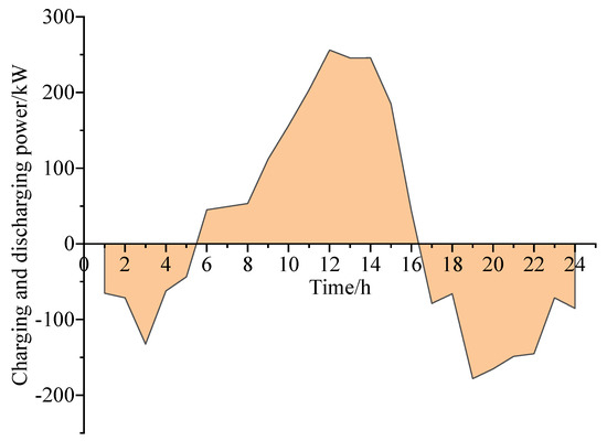
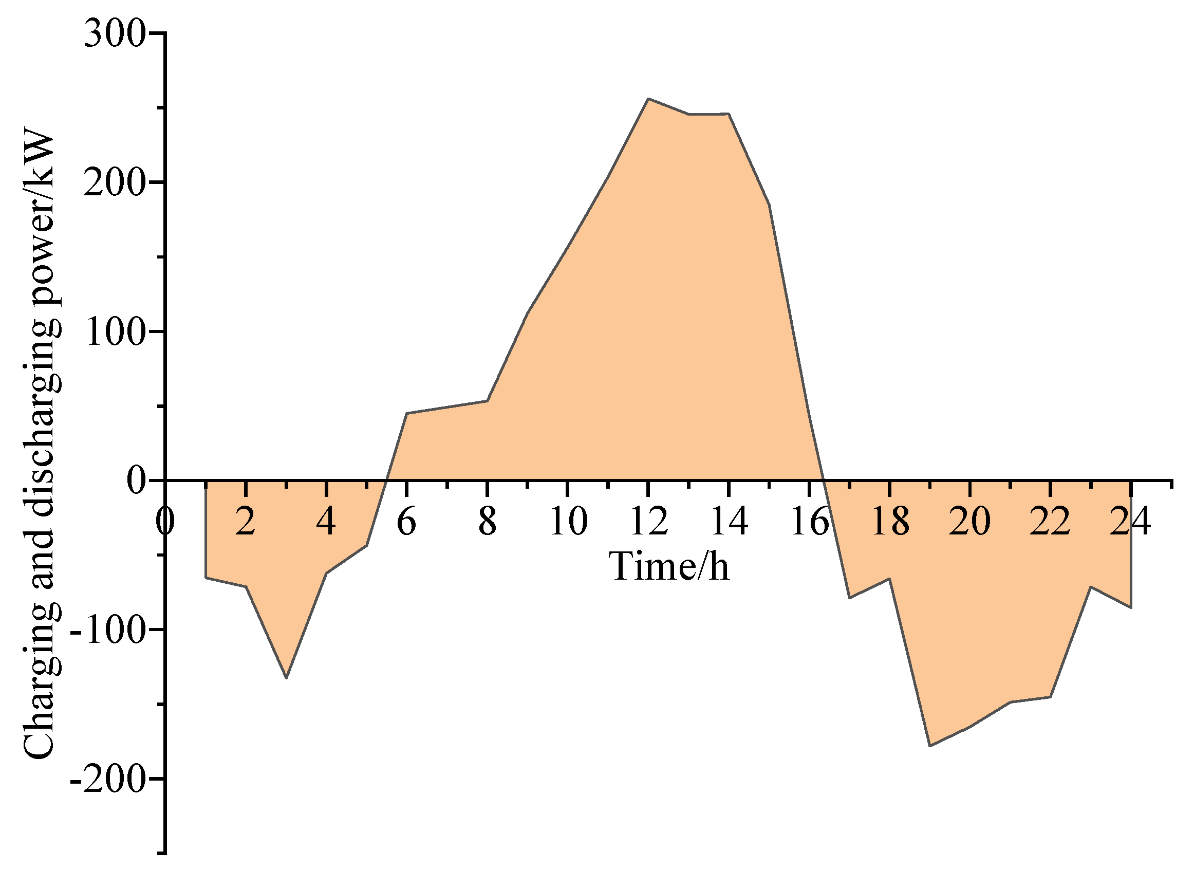
Figure 10 and Figure 11 illustrate the voltage fluctuations at two PV-connected nodes, respectively. Figure 12 reflects the variation trend of the charging/discharging power of the energy storage system.

Figure 10. The voltage magnitude at node 9.

Figure 11. The voltage magnitude at node 27.

Figure 12. Charging/discharging power of the energy storage system.

Under the unoptimized scheme, the voltage magnitudes at PV-connected nodes 9 and 27 exhibit significant and high-frequency oscillations in response to fluctuations in PV output: voltage rapidly climbs during peak PV output periods and sharply declines during valley periods, with a peak-to-valley difference in voltage magnitude far exceeding that of the optimized scheme. Given that engineering requirements for voltage fluctuations in power systems stipulate a peak-to-valley difference of ≤0.05 p.u. and a fluctuation rate of ≤2%/h, the fluctuation metrics of the unoptimized scheme completely exceed these standards, resulting in sustained voltage instability in the system—this represents the most intuitive core defect of the unoptimized scheme. Excessively high voltage at PV-connected nodes can lead to surplus reactive power at those nodes; if not promptly addressed, this surplus reactive power can propagate through the grid, triggering a cascaded voltage increase at adjacent nodes and creating regional overvoltage issues. Simultaneously, the disruption of reactive power balance further diminishes the grid’s voltage regulation capability, making it difficult for the system to swiftly restore voltage stability in the event of subsequent sudden load increases or sharp declines in PV output, thereby easily precipitating significant voltage drops and seriously threatening the safe and stable operation of the power grid.

Voltage control at PV connection nodes is challenging primarily due to the intermittent and fluctuating nature of PV output, which leads to frequent changes in nodal power. Traditional voltage regulation methods struggle to respond quickly to such dynamic variations, especially under extreme weather conditions or fault scenarios, where power supply–demand imbalances can further exacerbate voltage fluctuations. By generating multi-scenario PV output data using the TimeGAN model and employing k-means clustering to screen typical and extreme scenarios, a multi-scenario robust optimization model incorporating flexible adjustment resources has been constructed. The use of an improved Harris Hawks Optimization algorithm for global optimization enables the voltage control strategy to dynamically adapt to power fluctuations under different scenarios, significantly enhancing voltage stability. The flexibility of energy storage systems is reflected in their rapid switching capability between charging and discharging states, allowing them to store excess electrical energy during peak PV output periods to prevent overvoltage and release energy during low output or high load periods to support voltage. Additionally, by guiding user-side load adjustments through demand response models and time-of-use electricity pricing mechanisms, the system’s proactive regulation capability against voltage fluctuations is further strengthened.

To further verify the overall effectiveness of the method, multiple sets of verification cases were designed. By comparing voltage indicators before and after optimization, including voltage deviation rate and voltage stability margin, a comprehensive analysis was conducted on the applicable scenarios and performance boundaries of the method. The results are shown in Table 4.

Table 4. Comparison of voltage-related indicators before and after optimization.

Network Size	Mean Voltage Deviation Rate Before Optimization/%	Mean Voltage Deviation Rate After Optimization/%	Rate of Change	Voltage Stability Margin Before Optimization	Voltage Stability Margin After Optimization	Rate of Change
IEEE-14	2.8	1.9	−32.1%	0.85	0.89	+4.7%
IEEE-33	3.5	2.7	−22.9%	0.82	0.84	+2.4%
IEEE-118	4.2	3.9	−7.1%	0.78	0.79	+1.3%
Penetration Rate	Mean Voltage Deviation Rate Before Optimization/%	Mean Voltage Deviation Rate After Optimization/%	Rate of Change	Voltage Stability Margin Before Optimization	Voltage Stability Margin After Optimization	Rate of Change
10%	2.1	1.5	−28.6%	0.88	0.91	+3.4%
30%	4.0	3.2	−20.0%	0.80	0.82	+2.5%
50%	5.7	5.5	−3.5%	0.75	0.75	0%

In networks of all sizes, the core voltage indicators show positive improvements after optimization, verifying the method’s universality. However, as the network size increases, the positive effect of optimization on voltage weakens. For instance, in the IEEE-118 node system, the voltage deviation rate decreases by only 7.1%. This is because large-scale networks exhibit strong node coupling, leading to an exponential increase in the constraint dimensions for multi-scenario robust optimization. Consequently, the global search efficiency of the improved HHO algorithm declines, and the voltage optimization effects on some nodes are offset by the overall network complexity. In the IEEE-33 node system, under certain extreme scenarios, such as a sudden drop in PV output or a sudden increase in load, the voltage deviation rate of some local nodes rises from 2.9% to 3.1% after optimization, indicating a loss of positive impact. Nevertheless, the average value across all scenarios still shows positive improvement, suggesting that non-absolute positive effects are isolated cases in extreme local scenarios and do not undermine the overall effectiveness of the method. When the PV penetration rate is ≤30%, optimization has a significant positive impact on voltage. However, when the penetration rate increases to 50%, there is no improvement in the voltage stability margin, and the voltage deviation rate decreases by only 3.5%, indicating a near-disappearance of the positive impact. Under high penetration rates, during specific periods such as midday peak PV output, the optimization strategy aims to balance the overall network power by reducing reactive power compensation at some nodes. This results in an increase in the voltage deviation rate at those nodes from 5.6% to 5.8%. Nonetheless, the average value across all periods remains better than before optimization. The method demonstrates significant voltage optimization effects in scenarios with low to medium renewable energy penetration rates. In high-penetration scenarios, it requires the integration of flexible devices such as energy storage and SVGs to strengthen constraints and maintain positive impacts. The proposed method possesses both theoretical and technological potential for extension to larger-scale power networks. Its core framework is modular and scalable, with improvement ideas for key technical components tailored to the characteristic requirements of large-scale networks: the scenario generation and analysis module can be tuned to adapt to multi-node scenarios; the optimization model framework is universal and can be extended by adding constraint dimensions and parameters; and the improvement ideas for the solution algorithm can support large-scale solutions, such as introducing strategies like parallel computing. However, the method itself has inherent limitations, including a relatively singular focus on scenario generation objects, narrow consideration of non-ideal information transmission, deviations between model assumptions and actual conditions, and a lack of consideration for dynamic transient characteristics. During its extension, it also faces unique limitations such as decreased algorithm solution efficiency, difficulties in acquiring and integrating multivariate data, complex coordination and control of flexible regulation resources, and increased challenges in balancing robustness and economy.

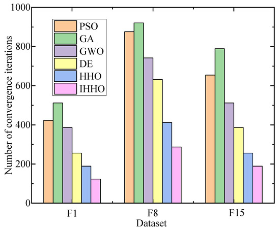
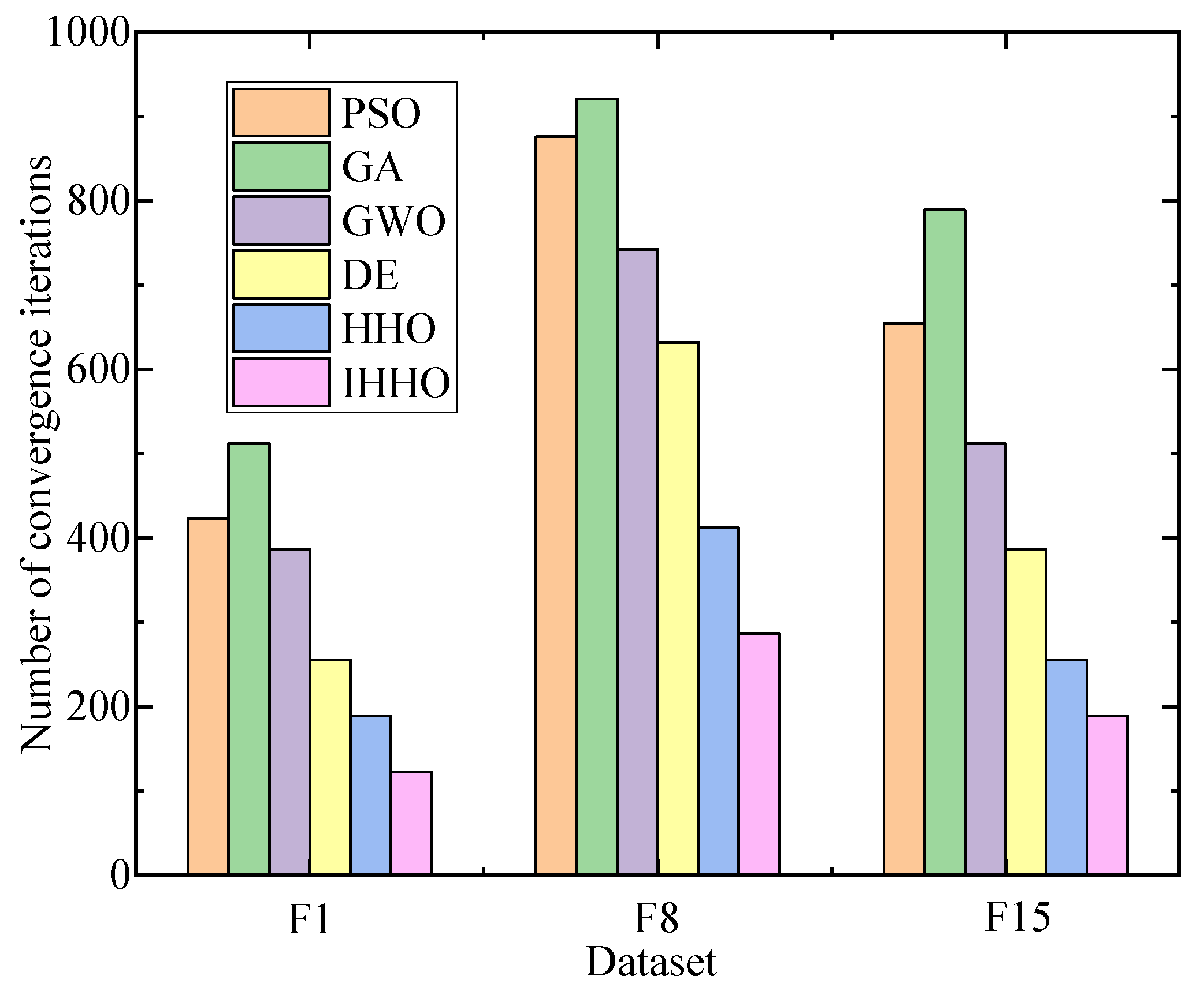
To further demonstrate the convergence performance of the algorithm, this paper selects the CEC2017 benchmark set, choosing unimodal function F1, multimodal function F8, and composite functions F15 and F23, with the dimensionality set to 30. For PSO, the inertia weight w is set to 0.729, and the cognitive coefficient is set to 1.494. GA employs tournament selection, single-point crossover with a probability of 0.8, and uniform mutation with a probability of 0.1. In GWO, the convergence factor a decreases linearly, while in DE, the scaling factor F is set to 0.5, and the crossover probability is 0.9. The parameters are uniformly set as follows: population size N = 50, maximum number of iterations T = 1000, and 30 independent runs. The optimization accuracies of different algorithms are shown in Table 5 below.

Table 5. Optimization accuracy of different algorithms.

Algorithm	F1	F8	F15	F23
PSO	1.23 × 10−4	18.72	0.45	2.31 × 103
GA	2.56 × 10−3	25.41	1.32	3.02 × 103
GWO	8.74 × 10−6	12.15	0.12	1.87 × 103
DE	3.12 × 10−7	5.89	0.05	1.24 × 103
HHO	1.02 × 10−8	3.21	0.02	8.76 × 103
IHHO	9.87 × 10−10	0.89	0.00	5.42 × 103

The IHHO demonstrates an accuracy two orders of magnitude higher than DE on the unimodal function (F1), owing to chaotic initialization that avoids local optima. In the multimodal function (F8), the Lévy flight perturbation significantly enhances IHHO’s ability to escape local traps, reducing errors by 72% compared to HHO. Under the complex terrain of the composite function (F23), IHHO improves the probability of converging to the global optimum by 41% through dynamically adjusting its escape energy. Figure 13 illustrates the convergence speeds across different datasets.

Figure 13. Convergence speeds of different algorithms.

The IHHO achieves a 35% faster convergence speed than HHO on F1, as chaotic mapping uniformly covers the search space, accelerating early exploration. In F8, the long-jump characteristic of Lévy flight enables IHHO to skip ineffective regions, reducing the number of iterations by 30%. The standard deviation of IHHO over 30 runs on F8 is 0.12, significantly lower than HHO’s 0.45, indicating that the improved strategies enhance algorithm stability. IHHO has an average runtime of 1.2 s per run, which is 0.1 s longer than HHO due to Lévy flight computation but considerably lower than PSO’s 2.1 s and GA’s 2.8 s. On F1, chaotic initialization reduces the fitness variance of the initial population by 63%, preventing premature convergence. In F8, after introducing Lévy flight, the number of times the algorithm escapes local optima increases from 12 out of 30 runs for HHO to 25 out of 30 runs for IHHO.

7. Conclusions

Complex operating conditions of power systems severely threaten the secure and stable operation of power systems, especially under fault-related extreme scenarios. The decision-making approach proposed in this paper offers an effective solution to this problem. By generating a joint scenario set from historical operational data, a multi-scenario robust stochastic optimization model is constructed, taking advantage of the system’s flexible adjustment resources. Moreover, the introduction of an improved Harris Hawks Optimization algorithm successfully addresses the non-convex and nonlinear challenges of the model, enabling the search for the global optimal solution. The simulation results on the modified IEEE—33 bus test system validate the feasibility and effectiveness of the proposed method. The generated photovoltaic scenarios using the TimeGAN model exhibit a KL divergence of 0.037 and a Wasserstein distance of 0.082 when compared to historical data, indicating a high degree of similarity and distribution consistency. Furthermore, the model successfully captures 98.7% of power fluctuations. This research provides valuable insights and a practical framework for ensuring the secure and stable operation of power systems, and it holds great potential for further application and development in real-world power system management.

References

- Qiao, X.; Qi, Y.; Zheng, Z.; Wang, W. Approximate Opacity and Its Enforcement for Cyber-Physical Systems Based on Reinforcement Q-Learning. IEEE Trans. Ind. Cyber-Phys. Syst. 2026, 4, 1–11. [Google Scholar] [CrossRef] [Scilit]
- Cheng, Y.; Su, J.; Chang, X.; Li, Z.; Xue, Y.; Sun, H. Optimal Operation of Integrated Electricity and Heat Energy Systems Considering Cyber-Physical Interaction. IEEE Trans. Smart Grid 2026, 17, 205–216. [Google Scholar] [CrossRef] [Scilit]
- Liu, A.; Ren, Y.; Pang, Z.-H.; Niu, B. Fixed-Time Secure State Estimation for Cyber-Physical Systems With Multi-Channel Transmission Under DoS Attacks. IEEE Trans. Circuits Syst. II Express Briefs 2024, 71, 3805–3809. [Google Scholar] [CrossRef] [Scilit]
- Chatterjee, A.; Huang, H.; Malak, R.; Davis, K.R.; Layton, A. Extending Ecological Network Analysis to Design Resilient Cyber-Physical System of Systems. IEEE Open J. Syst. Eng. 2024, 2, 38–49. [Google Scholar] [CrossRef] [Scilit]
- Qi, J.; Luo, X.; Fang, C.; He, J. Securing Cyber-Physical Systems Under Periodic Detection: Optimal Stealthy Linear Attack and Countermeasure. IEEE Trans. Control. Netw. Syst. 2025, 12, 2505–2517. [Google Scholar] [CrossRef] [Scilit]
- Zhao, D.; Shi, Y.; Ding, S.X.; Li, Y.; Fu, F. Replay Attack Detection Based on Parity Space Method for Cyber-Physical Systems. IEEE Trans. Autom. Control. 2025, 70, 2390–2405. [Google Scholar] [CrossRef] [Scilit]
- Ma, J.; Zhang, H.; Zhang, J.; Guo, X. Event-Based Adaptive Fault-Tolerant Control for Nonlinear Cyber-Physical Systems via Intermittent Available Signals. IEEE Trans. Autom. Sci. Eng. 2025, 22, 19850–19859. [Google Scholar] [CrossRef] [Scilit]
- Li, Y.; Ge, Y.; Zhao, Y.; Xu, T.; Abdennebi, M.; Zhu, M. Methods for Evaluating Critical Lines and Nodes in Cyber–Physical Power Systems From Three Network Perspectives. IEEE Syst. J. 2024, 18, 1987–1998. [Google Scholar] [CrossRef] [Scilit]
- Qu, Z.; Wang, P.; Li, J.; Georgievitch, P.M.; Wang, Y. A Globally Cooperative Recovery Strategy for Cyber-Physical Power System Based on Node Importance. IEEE Access 2024, 12, 179–191. [Google Scholar] [CrossRef] [Scilit]
- Yang, X.; Li, T.; Long, Y.; Yang, H. Secure Fault-Tolerant Control for Nonlinear Cyber-Physical Systems Against Multiple Threats. IEEE Trans. Autom. Sci. Eng. 2025, 22, 15060–15069. [Google Scholar] [CrossRef] [Scilit]
- Mejdi, H.; Elmadssia, S.; Koubãa, M.; Ezzedine, T. A Comprehensive Survey on Game Theory Applications in Cyber-Physical System Security: Attack Models, Security Analyses, and Machine Learning Classifications. IEEE Access 2024, 12, 163638–163653. [Google Scholar] [CrossRef] [Scilit]
- Yang, M.; Zhai, J. Predictor-Based Decentralized Event-Triggered Secure Control for Nonlinear Cyber-Physical Systems Under Replay Attacks and Time Delay. IEEE Trans. Control. Netw. Syst. 2024, 11, 150–160. [Google Scholar] [CrossRef] [Scilit]
- Li, H.; Lu, M.; Mao, J.; Yu, X. The Interaction of Macroscopic Optimization and Microscopic Traffic Flow With Communication Uncertainty in Intelligent Vehicle Cyber–Physical System. IEEE Open J. Intell. Transp. Syst. 2025, 6, 1265–1281. [Google Scholar] [CrossRef] [Scilit]
- Haridas, R.; Sharma, S.; Bhakar, R.; Gu, C. A Novel Integrated Load Redistribution Attack Model to Induce Cascading Failures in Cyber Physical Systems. IEEE Trans. Ind. Cyber-Phys. Syst. 2025, 3, 454–463. [Google Scholar] [CrossRef] [Scilit]
- Xiahou, K.; Du, W.; Xu, X.; Lin, Z.; Liu, Y.; Liu, Z.; Wu, Q. Resilience Assessment for Hybrid AC/DC Cyber-Physical Power Systems Under Cascading Failures. IEEE Trans. Reliab. 2025, 74, 3442–3453. [Google Scholar] [CrossRef] [Scilit]
- Zhou, B.; Su, R.; Zang, T.; Li, C.; Tong, X.; Gong, Y. Resilience Assessment of Power-Thermal Systems Considering Coordinated Cyber and Physical Attacks. IEEE Internet Things J. 2025, 12, 40159–40175. [Google Scholar] [CrossRef] [Scilit]
- Zhou, L.; Wang, Y.; Wu, Y.; He, S.; Song, Z. Quality-Relevant Modeling and Monitoring of Industrial Cyber-Physical Systems: The Semi-Supervised Dynamic Latent Variable Models. IEEE Trans. Ind. Cyber-Phys. Syst. 2025, 3, 39–47. [Google Scholar] [CrossRef] [Scilit]
- Bi, Y.; Wang, F.; Ding, P.; Wang, T.; Qiu, J. Multivariable Adaptive Super-Twisting Sliding Mode Resilient Control for Uncertain Nonlinear CPSs Against Actuator and Sensor Attacks. IEEE Trans. Autom. Sci. Eng. 2025, 22, 9039–9048. [Google Scholar] [CrossRef] [Scilit]
- Phillips, S.C.; Taylor, S.; Boniface, M.; Modafferi, S.; Surridge, M. Automated Knowledge-Based Cybersecurity Risk Assessment of Cyber-Physical Systems. IEEE Access 2024, 12, 82482–82505. [Google Scholar] [CrossRef] [Scilit]
- Xu, Q.; Li, X.; Jiang, Y.; Zhu, S.; Yang, B.; Chen, C.; Duan, S.; Guan, X. Transportation-Energy-Communication Integrated Management of Ship Cyber-Physical Systems Against Cyber Attacks. IEEE Trans. Smart Grid 2025, 16, 2518–2528. [Google Scholar] [CrossRef] [Scilit]
- Alvarez-Alvarado, M.S. Quantum Computing for Reliability Assessment of SCADA With Continuous Penetration Testing and High Penetration of Cyber–Physical Attacks. IEEE Trans. Smart Grid 2025, 16, 5392–5403. [Google Scholar] [CrossRef] [Scilit]
- Li, H.; Tang, T. Comprehensive Evaluation About Functional Elements of Intelligent Vehicle Cyber Physical System Based on the Normal Cloud Model. IEEE Syst. J. 2024, 18, 580–589. [Google Scholar] [CrossRef] [Scilit]
- Vincent, E.; Korki, M.; Seyedmahmoudian, M.; Stojcevski, A.; Mekhilef, S. Reinforcement Learning-Empowered Graph Convolutional Network Framework for Data Integrity Attack Detection in Cyber-Physical Systems. CSEE J. Power Energy Syst. 2024, 10, 797–806. [Google Scholar] [CrossRef] [Scilit]
- Wang, Y.; Wei, Z.; Liu, R. A Novel Proactive Defense Strategy Design for Cyber-Physical Systems in the Presence of FDI Attacks. IEEE Access 2025, 13, 86487–86497. [Google Scholar] [CrossRef] [Scilit]
- Liu, M.; Feng, Q.; Hai, X.; Zhang, Q.; Wen, C.; Khong, A.W.H. Collaborative Multiobjective Decisions for Cyber-Physical Production Systems Under Time-Varying Demands. IEEE Trans. Cybern. 2025, 55, 2643–2656. [Google Scholar] [CrossRef] [Scilit]
- Li, X.; Shang, R.; Zhao, Q.; Zhang, Y.; Liu, J.; Wu, C.; Guo, P. A Unified Online Assessment Framework for Pre-Fault and Post-Fault Dynamic Security. Energies 2026, 19, 673. [Google Scholar] [CrossRef] [Scilit]
- Zhang, C.; Wang, D.; Zhang, W.; He, L.; Zhou, K.; Li, J.; Zhu, L.; Zhou, B.; Zhou, Q.; Shuai, Z. A Novel Optimal Power Flow Method Considering Interval Uncertainties Under High Renewable Penetration Based on Security Limits Definition. IEEE Trans. Sustain. Energy 2025, 17, 926–938. [Google Scholar] [CrossRef] [Scilit]
- Available online: https://data.nlr.gov/ (accessed on 24 February 2026).
- Available online: https://power.larc.nasa.gov/ (accessed on 24 February 2026).
Disclaimer/Publisher’s Note: The statements, opinions and data contained in all publications are solely those of the individual author(s) and contributor(s) and not of MDPI and/or the editor(s). MDPI and/or the editor(s) disclaim responsibility for any injury to people or property resulting from any ideas, methods, instructions or products referred to in the content. |
© 2026 by the authors. Licensee MDPI, Basel, Switzerland. This article is an open access article distributed under the terms and conditions of the Creative Commons Attribution (CC BY) license.