


Abstract
In pico-hydropower, the use of pumps as turbines is a cost-effective solution, especially for remote areas. The abundant seawater makes it a good fluid for pumped storage. The operation of centrifugal pumps in normal and reverse modes involves thickness loss because of solid particle concentration and vapor cavitation. Some research has been performed to predict cavitation in centrifugal pumps, but this issue still exists in several pico-hydropower plants. Therefore, to analyse the synergy between erosion and cavitation in a seawater centrifugal pump, we performed a CFD analysis to compute the effect of material mass loss due to erosion on cavitation risk. The Euler–Lagrangian method was used to track the released particles combined with the RNG k-ε turbulence model. The first part studied the effect of the surface mean roughness height (Ra) on the performance of the centrifugal pump. Increasing Ra from 0 to 15 μm decreases the pump hydraulic efficiency from 93% to 91%, respectively. The second analysis focused on the distribution of erosion thickness and its temporal evolution for 40 μm and 50 μm particles. For both the pump mode and the turbine mode, the erosion thickness is a polynomial function of power 2 with time. The most eroded regions are the blade leading edge (LE) and the blade trailing edge in pump and turbine mode, respectively. The last section focuses on analysing the effect of erosion thickness on cavitation damage. As the surface roughness increases, the cavitation damage power increases. The cavitation power risk increases from 111 kW to 156 kW in pump mode. In turbine mode, when the erosion thickness is between 0.0011 μm and 0.0022 μm, the cavitation damage is the same, approximately 170 kW, whereas the total gas distribution is uniformly distributed in the blade channel. With respect to seawater, the NPSHr increased compared with that with freshwater, from 3.35 m to 3.67 m.
1. Introduction
A centrifugal pump is composed of an impeller and a volute to carry fluid to the penstock. The impeller is composed of blades that transport the fluid in the blade channel by increasing its pressure. Pump performance depends on the blade geometry, incidence loss, flow area (Q), and specific speed (ns) [1]. Most studies of centrifugal pumps focus on analysing the performance drop. On the other hand, failure or blade cracking can occur because of erosion, corrosion, and cavitation. Understanding the causes and prevention of centrifugal pump failure is crucial. Knowledgeable erosion/cavitation can provide engineers or operators with good guidelines concerning the reliability and durability of the pump. Once the cause of failure is understood, we can establish effective maintenance strategies and make necessary cost adjustments [2].
Cavitation in hydraulic machines is the most critical issue and causes noise, pressure pulsation, vapor formation, and material fatigue. Some studies have been performed to predict the effect of cavitation inception coefficient on centrifugal pump characteristics, resulting in a decrease in efficiency [3,4,5]. However, seawater has a higher vapor pressure and viscosity than freshwater does, which may cause more cavitation risk. The presence of solid particles makes the blade surfaces more eroded and rougher, increasing the hydraulic efficiency of the impeller.
The work of [6] investigated the effects of particle concentration and particle shape on the blade thickness loss of a centrifugal pump impeller. A linear relationship between the particle concentration and erosion rate was found. Compared with natural water, seawater fluid has a different dynamic viscosity, which can alter the erosion rate under the same fluid working conditions. In addition, erosion is material removal by solid particle wall attack. This mass removal increases the blade surface roughness, which affects the friction factor (f).
In the literature, few papers have discussed cavitation in turbine mode. However, in the blade sections where low-pressure zones appear, cavitation can occur in turbine mode at the blade TE. In this case, the blade lifetime is affected by the number of pump turbine cycles (pump or turbine). The goal of this study is to use CFD simulations to provide good ideas about the blade locations where erosion and cavitation occur for a centrifugal pump operated as a pump and as a turbine. The use of seawater as a fluid in centrifugal machines is not largely discussed in the case of cavitation and erosion. In the first section, we study the effect of blade surface roughness on hydraulic efficiency. Afterward, the effect of blade thickness loss on cavitation damage is evaluated.
2. Methodology
2.1. Centrifugal Pump Design
A centrifugal pump is a turbomachinery machine used to transport liquid flow from one point to another by increasing its pressure. It contains an inlet stator, a rotating impeller, a diffuser, and a volute. The blades of the impeller can be backwards or forward. Owing to the fluid velocity at the inlet, the inlet static pressure is low at the blade suction side. Each centrifugal pump is designed for a given best efficiency point (BEP). In turbomachinery engineering, for water pumps and turbines, the dimensionless parameters are identified as follows:
From Equation (3), if we replace the water flow (Q) from the equation of pump power, we can obtain the following equation:
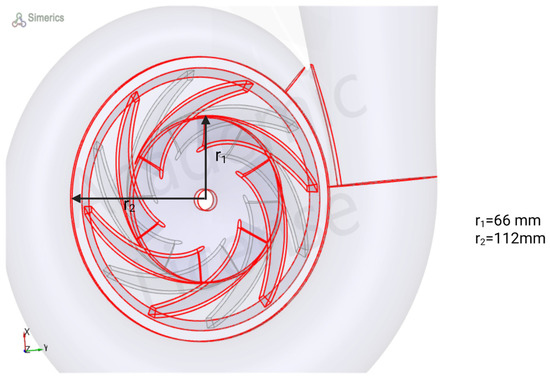
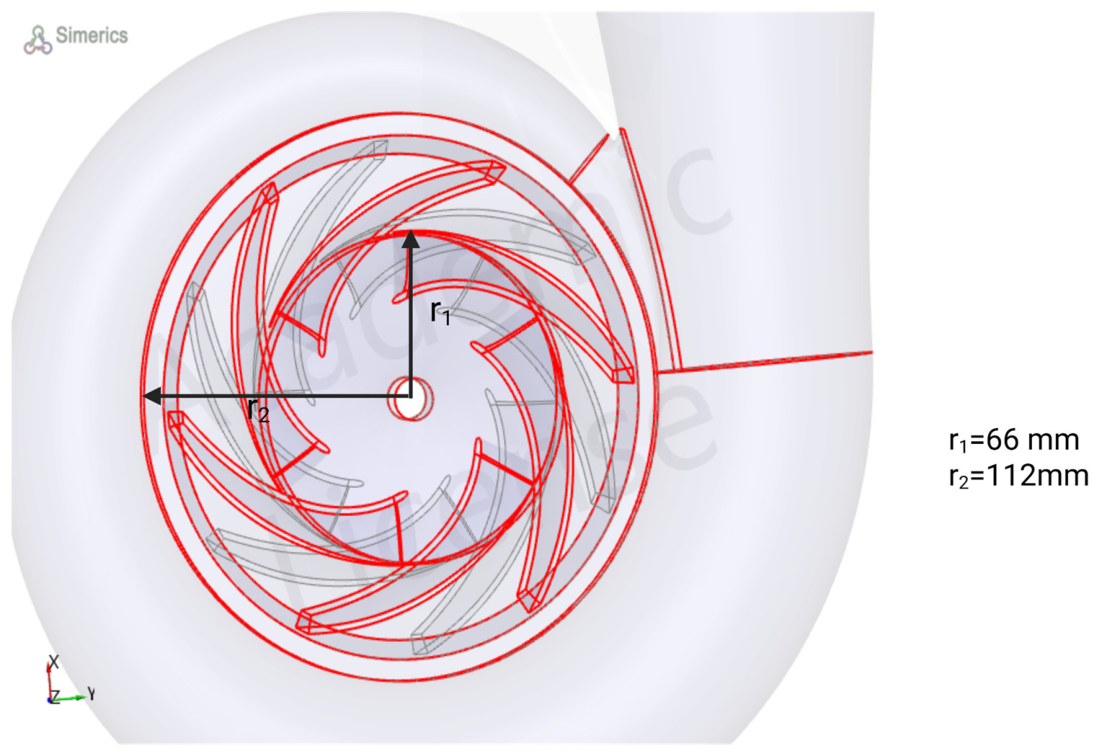
Given the data from Table 1, the specific speed is 49. The 3D geometry of the pump is generated by CFTurbo software (v2025 R2.2). Figure 1 summarizes the pump design parameters. The number of blades is 6 in the backwards direction.
Table 1.
Centrifugal pump design parameters.
Figure 1.
3D view of the centrifugal pump.
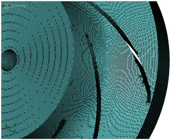
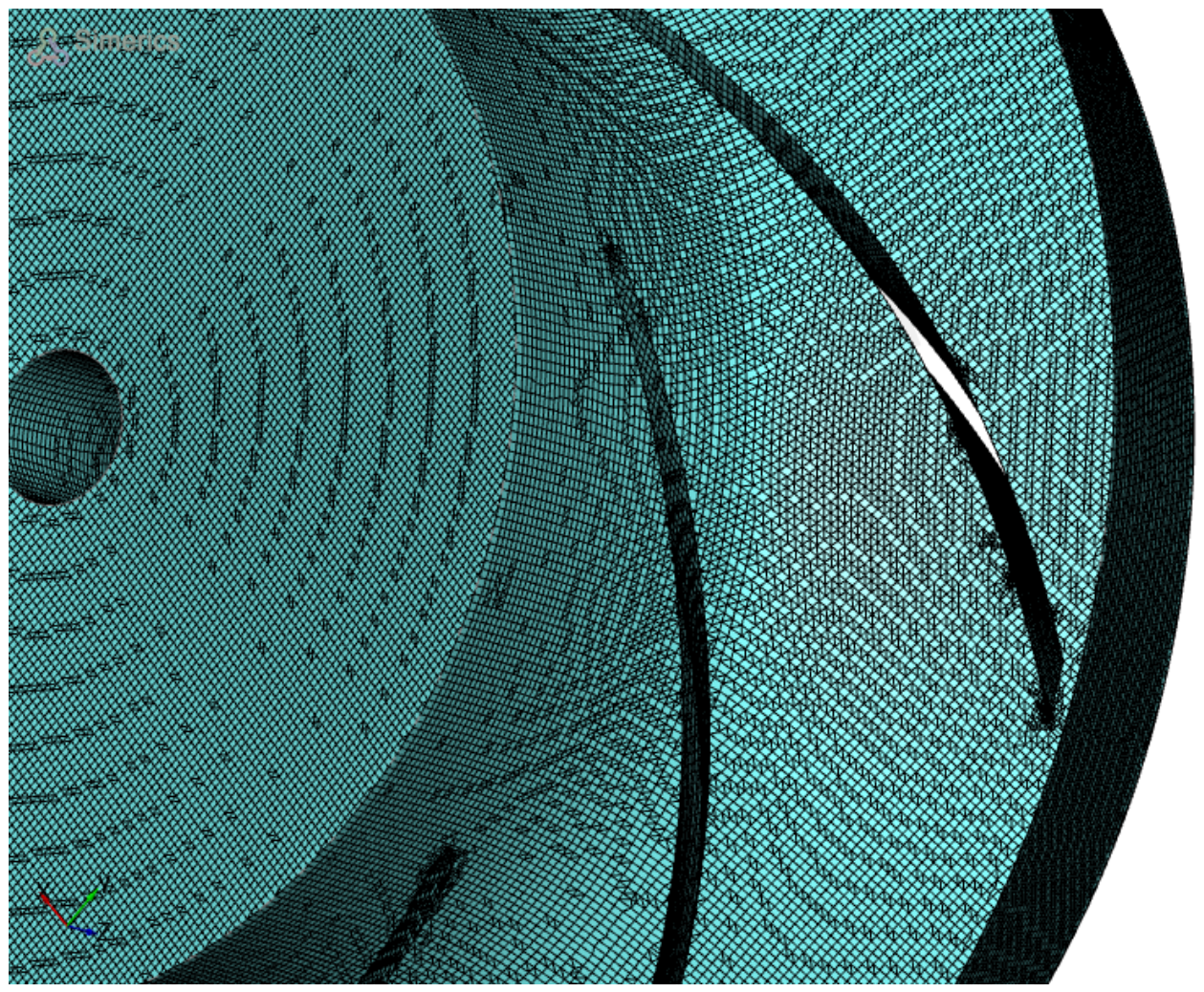
The binary meshing method was used to create the impeller mesh (Figure 2, Figure A1 and Table A1). The number of backwards blades is 6. At the blade channel entrance, the fluid enters with a low-velocity magnitude and leaves at a higher velocity at the blade trailing edge. The total pressure increases from the LE to the TE.
Figure 2.
Mesh generated by the binary meshing method at the TE. For more information, the mesh is presented in Appendix A. (There are two color: blue and black. Black is material surface whereas blue is meshing flow areas).
The power consumed by the pump is as follows:
2.2. Erosion Due to Solid Particles
Erosion is the removal of material mass because the solid particles slide on the blade wall. When a liquid flow contains solid particles, slurry erosion occurs. We generally have 4 types of erosion mechanisms:
- Cutting erosion: The material is removed when the particle strikes a material surface at a low impingement angle. The material mass is reduced by scouring or scraping against the sharp edges of the particles, resulting in the formation of short track lengths.
- Surface fatigue: Erosion mechanism at high strike angles and low speed. The mass loss is due to surface fatigue of the material.
- Plastic deformation: The erosion mechanism is due to the formation of flakes. When a particle sticks in the flake area, it continues to cut the material surface.
- Brittle fracture: If a particle attacks a brittle surface, it leaves the surface after cracking the subsurface.
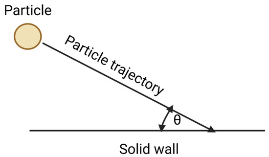
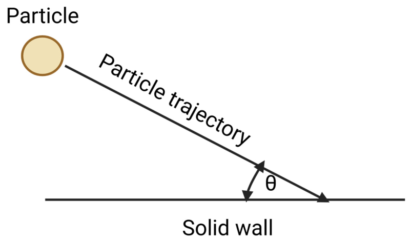
The quantity of removed mass depends on the flow regime, material mechanical properties, and solid particle parameters. However, when a particle hits a surface, it slides in the tangential direction of the flow. The movement of this particle depends on its impact velocity (Vimpact) and impingement angle (θ) (Figure 3). The data in Table 2 give the material’s mechanical properties.
Figure 3.
Collision between a solid particle and a wall on a smooth surface.
Table 2.
Wall material properties.
The work of [7,8] investigated the appearance of wear in the Francis Turbine runner because of the presence of solid particles. As the concentration of solid particles in water increases, the erosion rate increases.
Finnie developed an erosion model for ductile and brittle materials for determining the mechanism of slurry erosion. The maximum erosion rate occurs at an impingement angle of 30° [9].
Finnie and Grant Tabakoff [9,10] studied erosion wear in different cases. Finnie proposed an erosion model to compute the erosion rate (ER) according to Equation (2). The erosion rate is the ratio of the total removed mass divided by the eroded particle mass (Figure 4).
Figure 4.
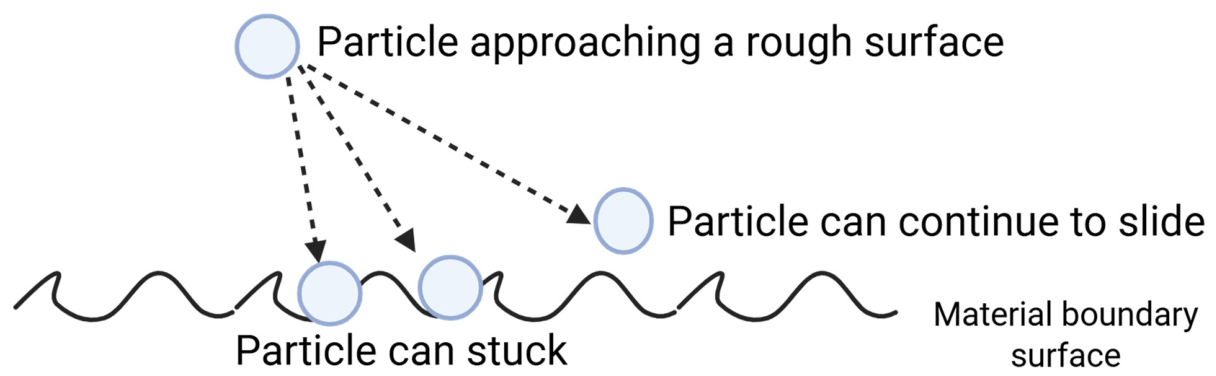
The effects of surface roughness on the erosion mechanism are as follows: (cure line: material surface boundary layer).
In this simulation, we assumed that the particle was perfectly spherical. The restitution ratios were 0.5. However, the kinetic energy loss of the particle before and after wall interaction is reduced. Given that liquids have higher density, we assumed that the initial particle velocity is the same as the fluid velocity. Table 3 shows the material properties and particles used for the erosion simulation.
Table 3.
Erosion parameters used with the Finnie model to compute the erosion thickness.
In the case of an eroded surface, the wall is considered a rough surface. The effect of surface roughness is shown in the figure below. However, in the presence of thickness loss, the particle can continue to slide in the wall direction or become stuck. This leads to a change in the erosion type, from abrasion to plastic deformation.
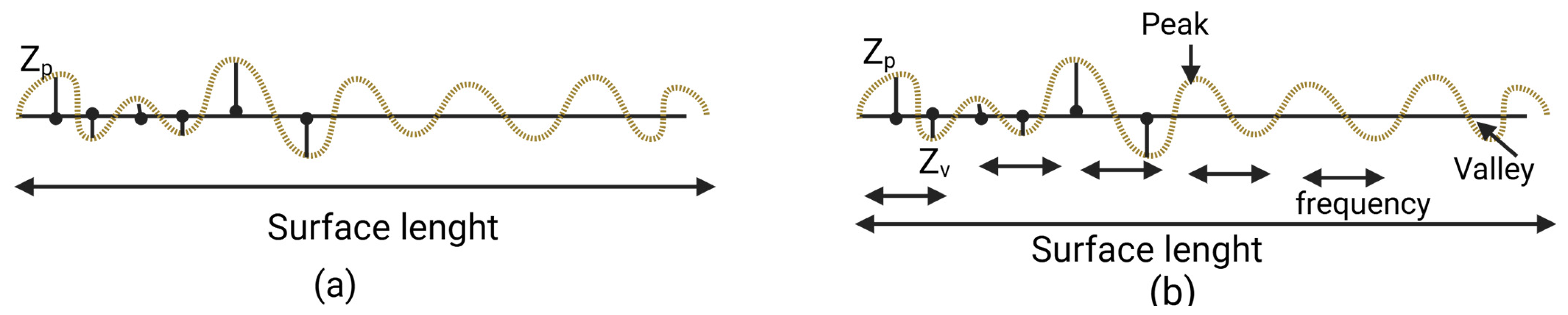
Two roughness heights are defined: the average surface roughness and the mean surface roughness (Figure 5).
Figure 5.
Average and mean surface roughness, respectively ((a) and (b)).
On a rough surface, we have peak and valley surface heights that change depending on the surface height. For the average roughness height, the surface roughness is defined as the average of the peak and valley surface values.
In the case of the mean surface roughness, the surface length is subdivided into (n) small lengths to detect the peak and valley heights. The Ra is calculated as follows:
In this study, we used the average surface roughness as the input for the wall roughness height.
2.3. Cavitation Model
Cavitation is the formation of a vapour fraction in liquid flow. In contrast to boiling, the phase change from liquid to vapour is due to a pressure drop in each region. In a centrifugal pump impeller, owing to rotation and its associated centrifugal forces, the static pressure at the blade inlet is lower. In thermodynamics, the pressure at which the vapour appears is the vapour pressure (pv). The onset of the cavitation limit generally occurs with a critical value, which is the incipient cavitation constant given as follows:
As the liquid passes through the impeller channel, the pressure gradient changes. Near the LE of the impeller blades on the suction surfaces, a rapid increase in velocity and a corresponding decrease in pressure occur. If the static pressure of the liquid drops below the vapour pressure, then cavitation occurs. The fluid then moves into the impeller; within the blade passage area, the pressure increases. This pressure rise causes the collapse of the air cavitation bubbles, and the resulting implosion of the bubbles and consequent shock waves can cause pitting of the impeller blades and, eventually, structural failure.
In the pump impeller inlet, the static pressure is likely equal to the vapour pressure:
The typical range of the value of σ is 0.2 to 0.4 [11]. From Equations (10) and (4), one can compute the optimum conditions at the pump inlet conditions as follows:
From Equation (9), the non-cavitation flow corresponds to a high cavitation number linked to a high reference pressure. That is, the pressure distribution is very high compared with the vapour pressure. The Thoma coefficient is the minimum coefficient of cavitation damage. Below this value, erosion causes significant damage [12]. The value of σ can be calculated as follows:
In this study, the constant gas model is considered [13,14] on the basis of the Singhal et al. model. This model assumes that in the cavitation flow, the presence of non-condensable gas (NCG) is ideal. The density follows the ideal gas law:
The volume gas fraction is defined as follows:
The non-condensable mass gas fraction fg is constant and typically ranges from to 23 ppm. In the presence of the vapour phase, the weighted density is
Since we are in the presence of an incompressible fluid, we assume that and ; from Equation (4), we have the following:
From mass conservation,
From Equations (5) and (6), we have the following:
The appearance of the vapour phase is a result of mass transfer from the liquid to the vapour phase. The amount of mass transfer is as follows:
Liquid phase:
Vapour phase:
Combining Equations (8) and (7), we have the amount of mass transfer from the liquid to the vapour phase:
The liquid fraction is as follows:
2.4. Turbulence Model
In this study, the RNG k-ε model was used to solve the full 3D Navier–Stokes equation.
In the case of an incompressible fluid, the density variation with time is 0.
To decompose the instantaneous average Navier–Stokes equation variables, we use Reynolds average Navier–Stokes (RANS) averages. The flow variable is composed of an average mean and a fluctuating component.
Inserting this equation into Equation (14) results in the following:
The appearance of the transport term should be solved by using k-ε models.
where is the turbulent kinetic energy. In this simulation, we used an RNG model that better describes the turbulent viscosity in low-Reynolds-number regions. The first term in the second term of Equation (16) corresponds to the turbulence production. This expression depends on turbulence, viscosity, modelling, and energy dissipation. In the RNG theory, the turbulence viscosity depends on the k–ε constants and swirl factor (w, vorticity index).
The discrete phase model (DPM) was used to track the particle motion from the release position at the outlet section.
FD: Drag forces.
- FG: Gravity forces
- FC: Coriolis forces
- FCentrifugal: Centrifugal forces.
3. Results
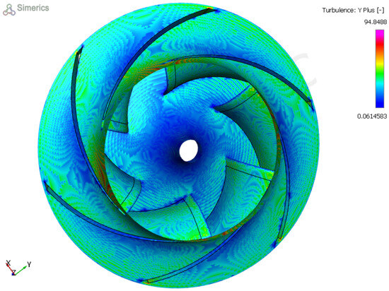
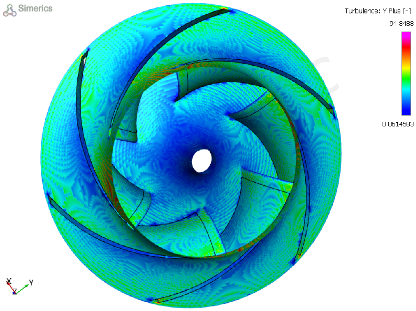
To better evaluate our model accuracy, we computed the Y+ value on the centrifugal pump side. Y+ is the nondimensional distance from the wall to the mesh. As much as this value is lower, the viscous force is dominant. At the same location of the boundary layer, with the same dynamic viscosity, changing the surface height will change the velocity gradient.
The value of Y+ is defined as:
where
The change in u+ with Y+ is a logarithmic function. When the value of y+ is less than 5, we assume that u+ is equal to Y+. In our case, the wall function shows a viscous and buffer sublayer, as illustrated in the figure below. The distribution of the Y+ values is displayed in the figure below (Figure 6). This means that our flow is dominated by viscous and turbulent forces.
Figure 6.
Y+ value distribution. From this distribution, the wall function is a sublayer viscous area.
3.1. Effect of Surface Roughness on the Impeller Efficiency
According to Colebrook’s White equation, in turbulent flow, as the relative surface roughness increases, the friction factor increases. To illustrate the effect of blade surface roughness on the impeller efficiency, we computed the impeller efficiency for different Ra. The table below shows a decrease in the impeller efficiency by 10% when the surface is changed from smooth to rough with Ra= 15 μm (Table 4).
Table 4.
Variation in the impeller efficiency with surface roughness. A decrease in efficiency is expected as Ra increases.
3.2. Comparison of Erosion Thickness Between Water and Seawater
Effect of the Operation Mode on Erosion Thickness
The erosion thickness is linearly related to the erosion density. It is defined as follows:
The thermophysical properties of water and seawater are listed below (Table 5). The dynamic viscosity of seawater with a salt concentration of 30 g/L is less than that of water. This causes high erosion thickness on the sides of the blade (Table 6).
Table 5.
Thermophysical properties of water and seawater.
Table 6.
Erosion thickness with water and seawater for particle sizes of 40 and 50 microns.
The erosion thickness is the material mass loss in the orthogonal direction of the wall. The material loss increases the surface roughness height, which affects the total efficiency. The efficiency decreases because of solid particle erosion. We changed the surface roughness in Simerics MP+ (version 6.0.17) after each time step by the maximum erosion thickness in the boundary layer (Table 7).
Table 7.
Blade surface roughness heights after 125 ms of pump operation.
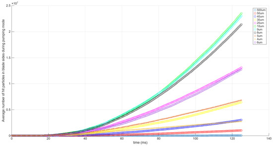
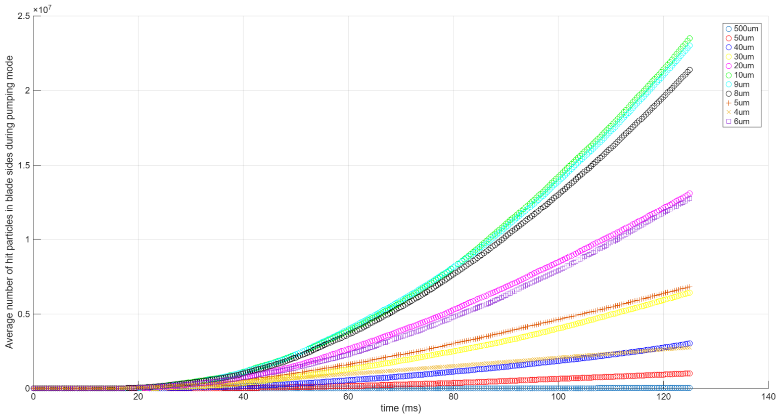
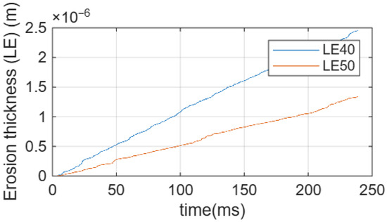
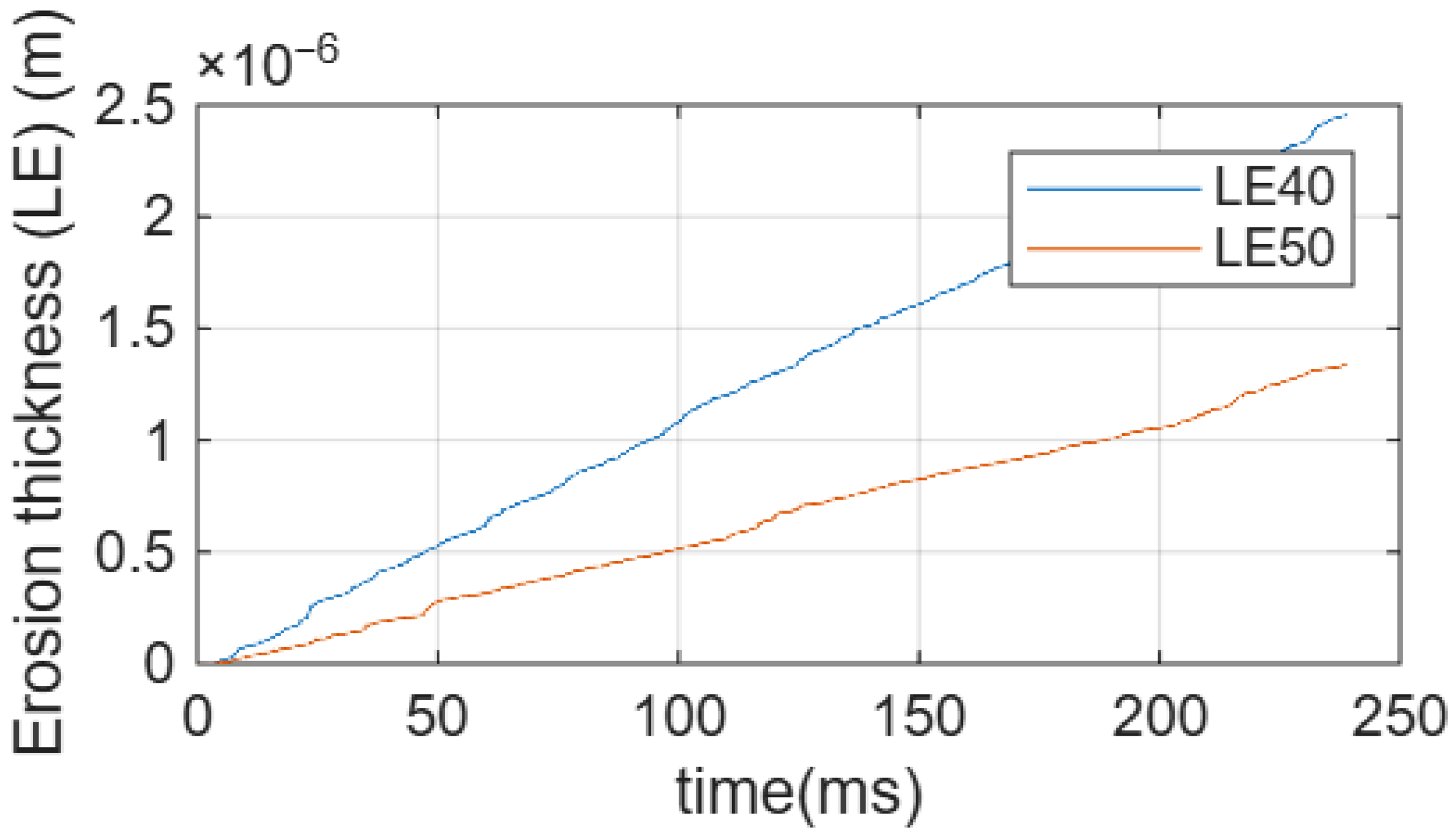
From the temporal evolution, we can see that the erosion thickness is a polynomial pump running time (Figure 7). This means that with these two sizes, the particles are parallel to the blade channel. In the case of seawater, when it passed from 40 to 50 microns, the erosion thickness increased (Figure 8). However, owing to the high density of the fluid and the kinetic energy of the particles, the particle leaves the blade channel more quickly than it does at 40 µm. However, using seawater as a fluid in a centrifugal pump designed with water under standard thermodynamic conditions reduces hydraulic efficiency. In our case, we passed from 0.897 to 0.896. In the blade leading edge boundary layer, the erosion thickness is linear with time (Figure 8), making this surface roughness more strongly impacted by erosion thickness loss (Figure 9).
Figure 7.
Temporal evolution of particle hit counts on blade sides for different particle sizes (pump mode). After a given operation time, the erosion thickness increases because the particles are parallel to the blade channel.
Figure 8.
Temporal evolution of erosion thickness at the blade leading edge with respect to particle size. The erosion thickness is linear with time.
Figure 9.
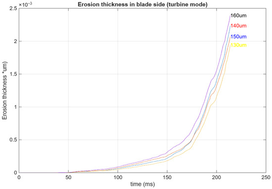
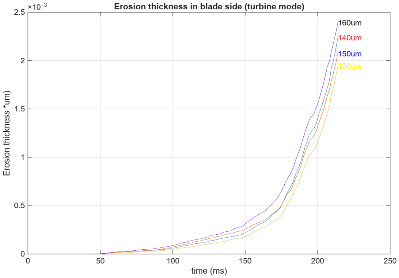
Erosion thickness on the blade sides in turbine mode. The erosion thickness loss is exponential with time.
3.3. Cavitation Damage
3.3.1. Pump Mode
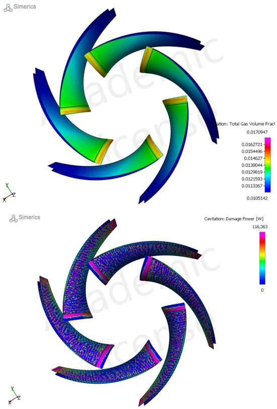
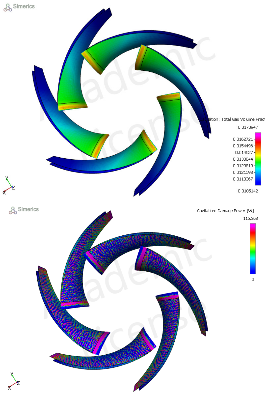
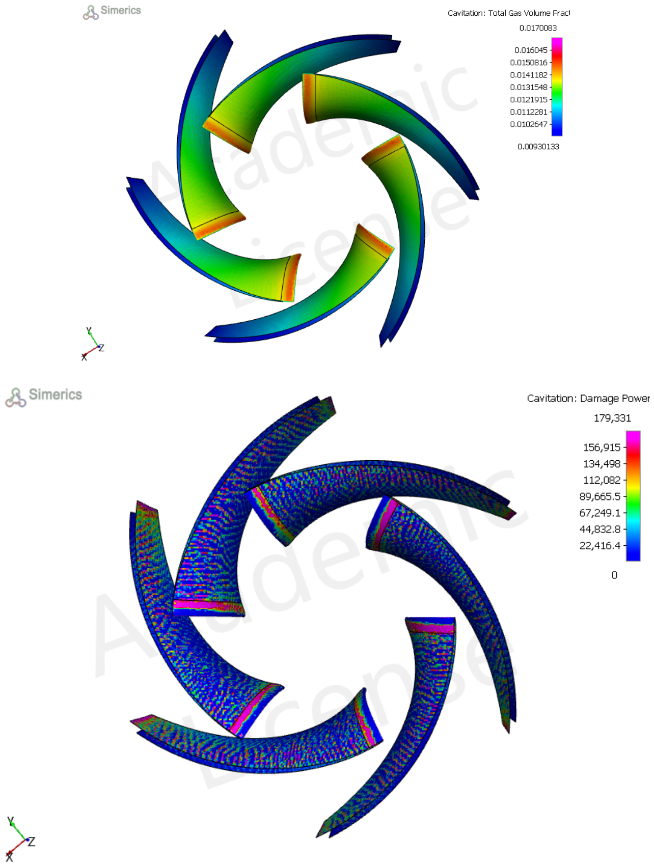
Erosion–cavitation in the pump mode strongly affects the inlet section. At the inlet section, the fluid enters a zone with high velocity and low pressure, creating a very low-pressure zone. Figure 10 shows the damage power in the blade LE section. From t = 238 ms to t =253 ms, the erosion thickness increases at the leading edge of the blade. As the erosion thickness increases, the flow pattern changes, causing changes in pump cavitation damage. However, the surface roughness changes according to the average erosion thickness. In Simerics, we used surface roughness as a variable with the corresponding erosion thickness in the given boundary layer (Figure 10 and Figure 11). For example, on the blade side, the surface roughness is equal to the erosion thickness caused by a particle size of 40 microns as follows: ThicknessBS = particle.40 µm.erosion_thickness@patch. “Pump-BladeSides” (Table 8).
Figure 10.
The total gas fraction and cavitation damage in the pump mode. The total gas mass fraction is greater at the blade LE because of the low-pressure zone. This zone has more cavitation risk in the pump mode.
Figure 11.
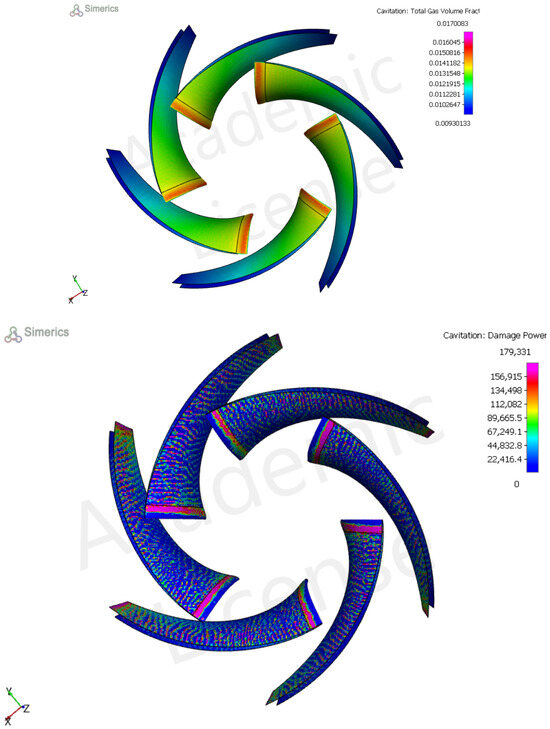
Total gas mass fraction and cavitation damage at t = 253 ms.
Table 8.
Erosion thickness on the blade leading edge and blade sides at t = 238 ms.
- particle.40 µm.erosion_thickness: the erosion thickness caused by a particle size of 40 μm
- patch. BladeSides: We obtain the value at the blade sides
- ThicknessBS: The blade roughness height corresponding to the given erosion thickness
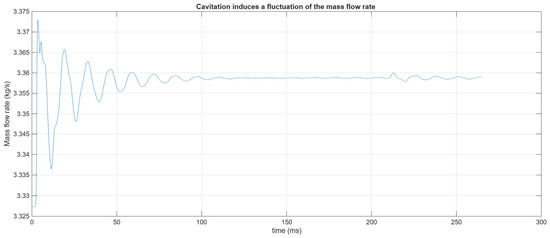
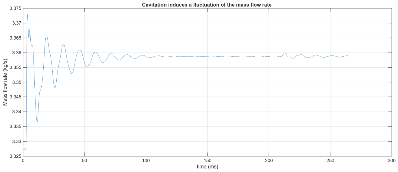
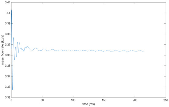
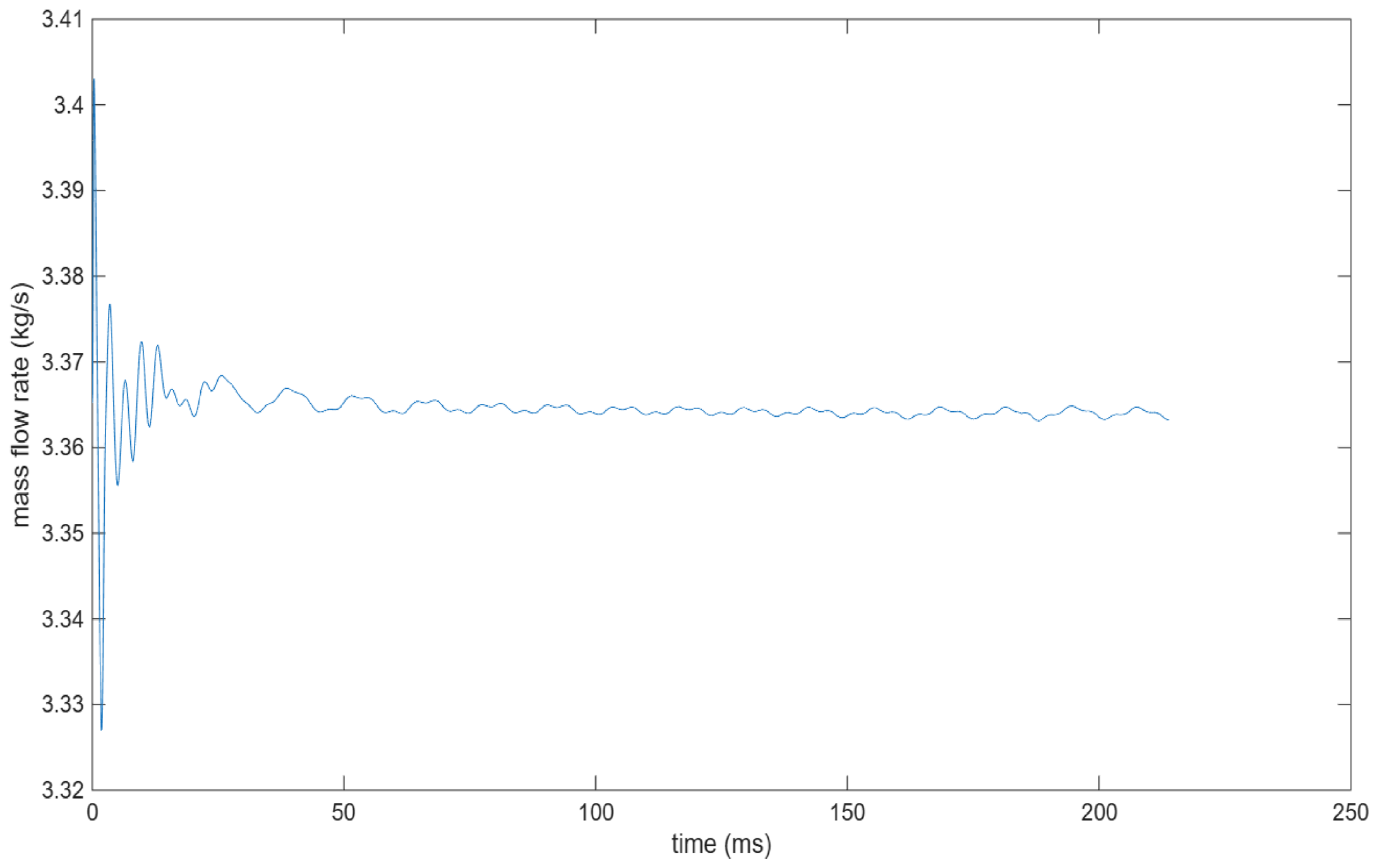
One consequence of the cavitation is that the mass flow rate is not constant. However, when the surface roughness increased significantly, our simulation revealed that some fluctuations were observed, as depicted in Figure 12. This means that the pressure on the sides of the blade fluctuates (Table 9).
Figure 12.
Mass flow rate at the pump outlet exposed to cavitation and erosion damage.
Table 9.
Erosion thickness in the blade leading edge and the blade sides at t = 253 ms.
The required NPSHr is greater in the case of seawater than in freshwater. However, the dynamic viscosity of seawater is higher than that of freshwater, causing more shear stress and friction losses. We run the tutorial of the Simerics tutorial of the centrifugal pump at Q = 0.012 m3/s, H = 10 m, and N = 2500 RPM. The NPSHr values for seawater are 3.67 m and 3.35 m, respectively (Table 10).
Table 10.
NPSHr values for a centrifugal pump used with freshwater and seawater.
To validate our results, the studies of [15,16,17] reported that the onset of cavitation occurs earlier in the case of seawater and increases as the salt concentration increases. The bubble size is larger in the case of seawater than in freshwater.
3.3.2. Pump as Turbine (PaT)
When the centrifugal pump operates in reverse mode, the flow attacks the blade TE with an incidence loss because of the difference between the blade outlet angle and flow angle. This incidence loss affects the erosion thickness, as only very large particles can resist flow.
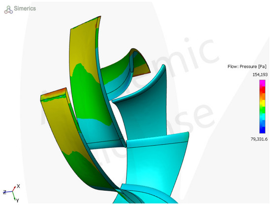
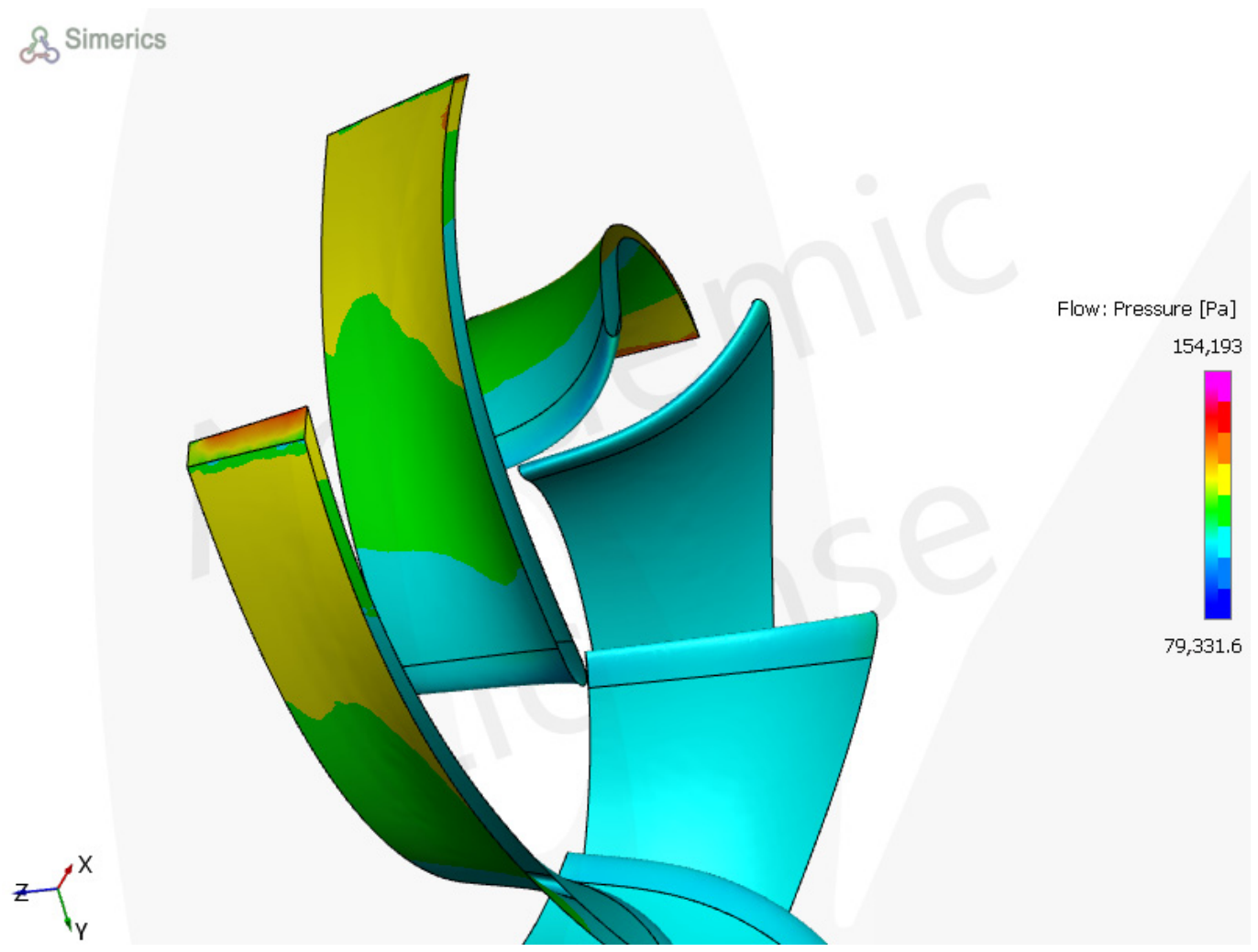
The distribution of the static pressure is not uniform in the blade channel, causing nonuniform free gas concentration (Figure 13). As the erosion thickness increased, the hydraulic efficiency of the PaT decreased. However, the erosion thickness loss at t = 193 ms and t = 202 ms increased from 0.0012 μm to 0.0022 μm, where the hydraulic efficiency decreased from 90% to 89.95%.
Figure 13.
Static pressure on the sides of the blade. Uniformity from blade TE to blade LE.
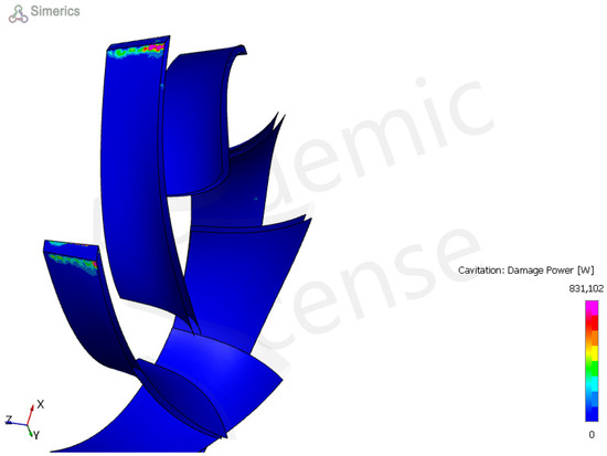
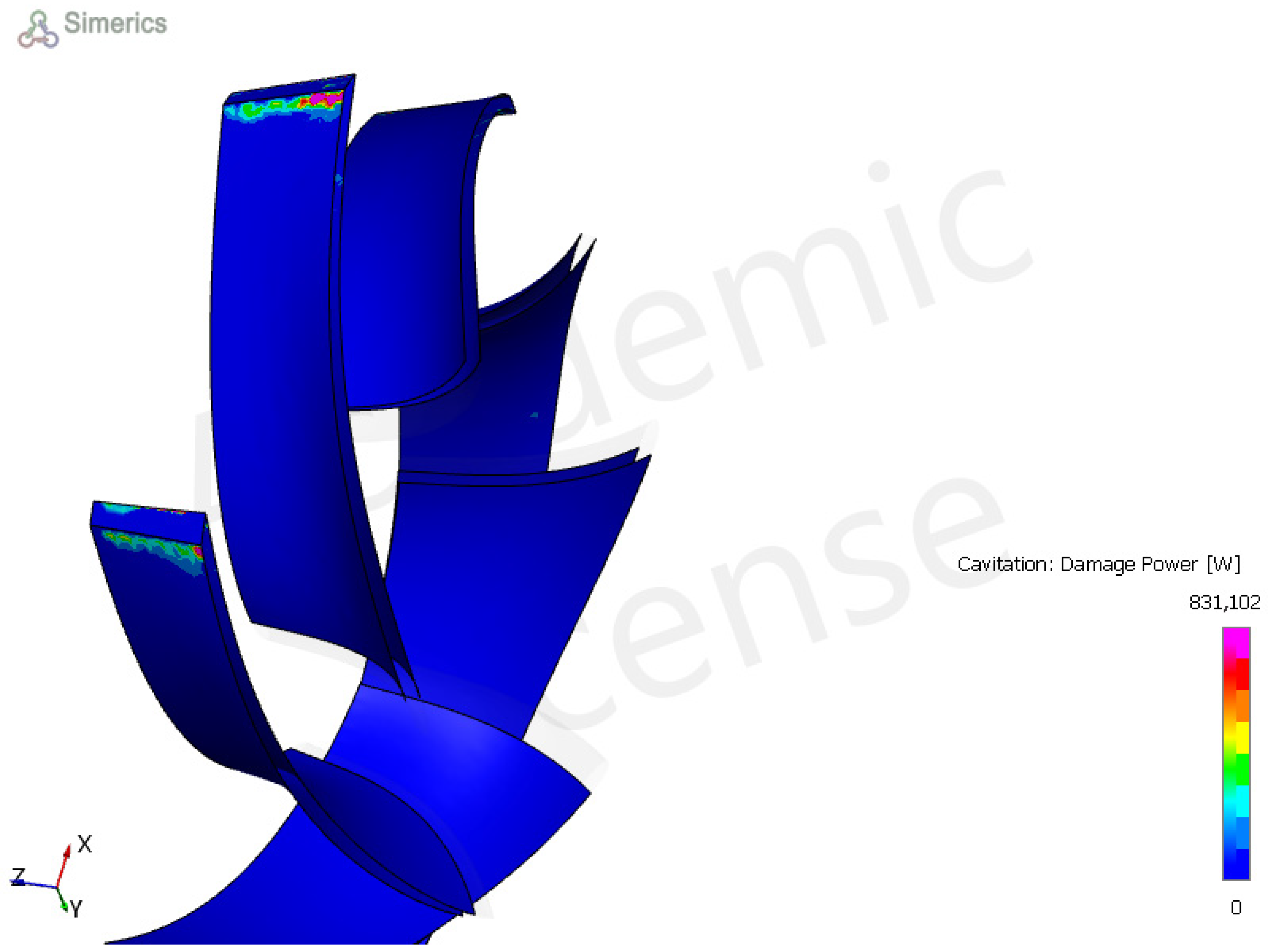
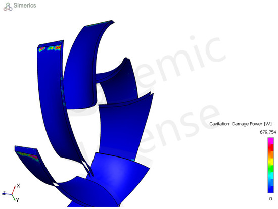
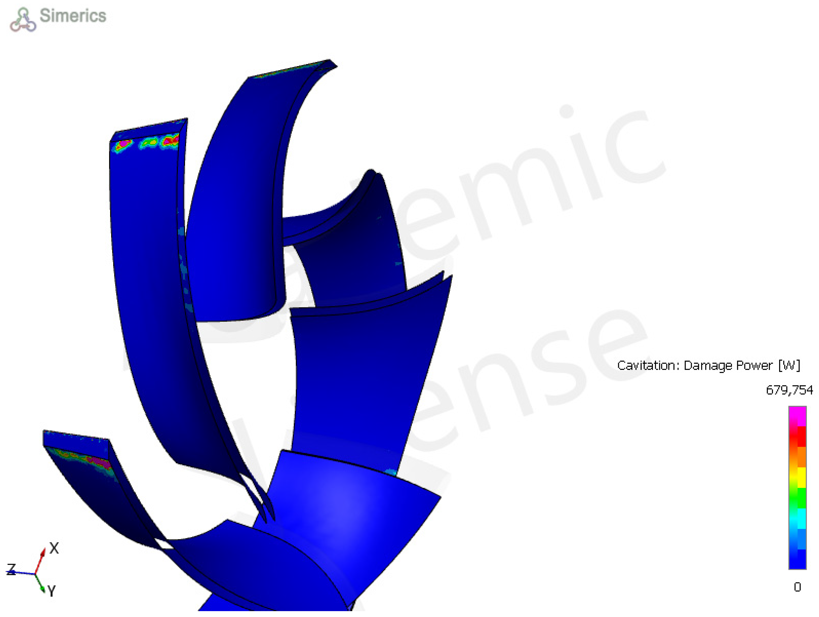
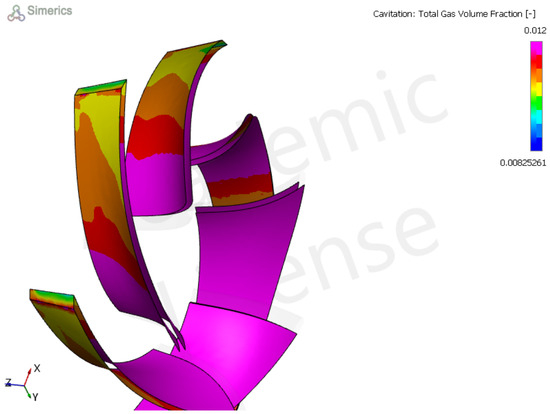
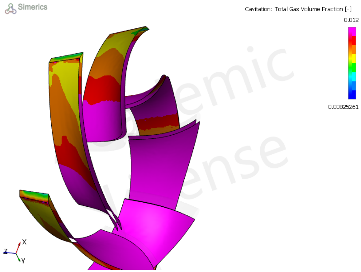
Our study revealed that in turbine mode, the mass flow rate fluctuates because of the synergistic effects of cavitation and erosion (Figure 14). The fluctuation in the mass flow rate leads to a fluctuation in the static pressure. In turbine mode, cavitation can occur at the blade TE and LE because of low static pressure (Figure 15, Figure 16 and Figure A2). A review by [13] revealed that flow separation occurs at the blade LE in turbine mode, causing high cavitation inception in this region.
Figure 14.
The gas damage power in turbine mode is t = 193 ms, ser = 0.0012 μm, ηp = 0.9.
Figure 15.
The gas damage power in turbine mode is t = 202 ms, ser = 0.0022 μm, ηp = 0.8995.
Figure 16.
The mass flow rate in the PaT operated under erosion–cavitation synergy.
Thoma’s coefficient is used to predict the cavitation risk in turbine mode. When Thoma’s coefficient is less than the critical coefficient, there is a cavitation risk. The critical Thoma’s coefficient is computed as follows:
In our case, the critical coefficient is 0.01, where the computed Thoma’s coefficient is 0.19.
4. Discussions
The performance of a centrifugal pump depends on its flow characteristics and geometry. However, the blade angle distribution fixed the magnitude of the relative velocity, which affected the impact velocity of the particles. The experimental results from [18] show that reducing the inlet relative velocity decreases the degree of cavitation damage. Another proposition is to increase the inlet static pressure slightly by using an inlet swirl. This will keep the inlet pressure above the fluid vapour pressure.
In turbine mode, travelling cavitation can occur on the blade section side to propagate the gas flow rate. However, in this cavitation type, the air bubbles flow in the blade direction. As illustrated in Figure 17, the gas fraction is distributed in the blade section.
Figure 17.
The gas volumetric fraction on the blade suction side in turbine mode. the gas bubbles travelled on the blade channel. The total gas mass fraction varies along the blade channel, which can cause cavitation to travel.
The work of [19] compared experimental and theoretical simulations of the effect of cavitation on the internal flow of a centrifugal pump. As the cavitation coefficient intensifies, the small vortex is considered in the flow regime in performance prediction.
5. Conclusions
In this study, we studied the erosion–cavitation synergy in a centrifugal pump operated as a pump and as a turbine. Erosion makes the wall surfaces rougher, which decreases the impeller efficiency.
The thickness loss increased with a polynomial function in the pump and turbine modes. The total free gas concentration was high at the blade LE section, causing high potential damage due to cavitation. As the erosion thickness increases, the degree of cavitation damage increases. In turbine mode, the cavitation damage is serious at the blade TE and blade LE, whereas the total free gas concentration is not uniform along the blade channel. The synergy between erosion and cavitation in a centrifugal pump is positive. As the thickness loss increases, the degree of cavitation damage increases.
The general conclusions below should be noted:
- As the surface roughness increases, the impeller efficiency decreases because of an increase in the friction factor.
- The erosion thickness depends on the particle size. For the pump, the temporal evolution ER is constant with particle sizes of 40 and 50 microns (particle go parallel to the blade channel), whereas it is exponential in turbine mode.
- The erosion thickness makes the impeller surface rougher. However, the particles slide in the flow direction where they cut the material wall surface. As the surface becomes rougher, the particles can continue their trajectory and become stuck, rebound or reflected.
- In pump mode, cavitation damage is more serious at the blade inlet because of low-static-pressure regions. In turbine mode, cavitation is more likely to occur at the blade Edges.
- In the case of seawater, cavitation onset occurs earlier than in freshwater.
Author Contributions
Conceptualization, J.E.M. and P.H.; methodology, J.E.M.; software, J.E.M.; validation, P.H., A.H. and F.B.; formal analysis, J.E.M.; investigation, P.H.; resources, J.E.M.; writing—original draft preparation, J.E.M.; writing—review and editing, J.E.M.; visualization, J.E.M.; supervision, P.H.; project administration, P.H. All authors have read and agreed to the published version of the manuscript.
Funding
This research received no external funding.
Data Availability Statement
The original contributions presented in this study are included in the article. Further inquiries can be directed to the corresponding author.
Conflicts of Interest
The authors declare that there are no conflicts of interest.
Abbreviations
| LE: | Blade leading edge |
| TE: | Blade trailing Edge |
| BS: | Blade sides |
| s: | Blade thickness loss (m) |
| e: | Blade thickness (m) |
| ER: | Erosion rate |
| erdensity: | Erosion density (kg/m2s) |
| θ: | Impingement angle (deg) |
| Hv: | Material Vickers’ index (Pa) |
| ρm: | Material density (kg/m3) |
| ρg: | Gas density (kg/m3) |
| ρp: | Particle density (kg/m3) |
| Vp: | Particle velocity (m/s) |
| z: | Position of the turbine (m) |
| He: | Effective pump head (m) |
| μt: | Turbulent viscosity (Ps.s) |
| N: | Rotational speed (rev/min) |
| Q: | volumetric flow of the fluid (m3/s) |
| : | shear stress at wall |
Appendix A
Mesh at the TE.
Figure A1.
Mesh quality at blade TE.
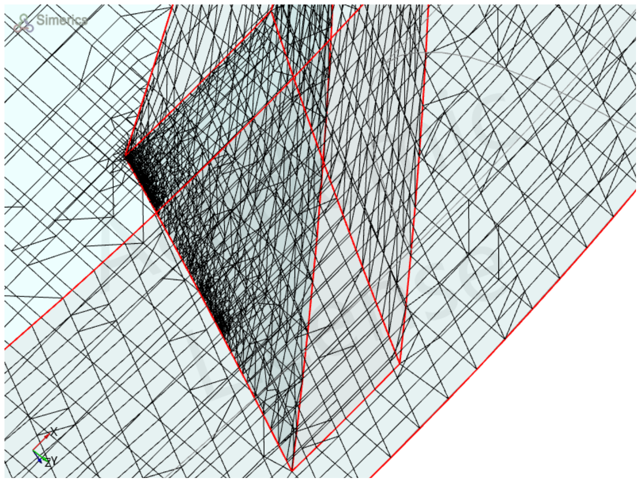
Figure A2.
Cavitation damage with total gas mass fraction (pump as turbine).
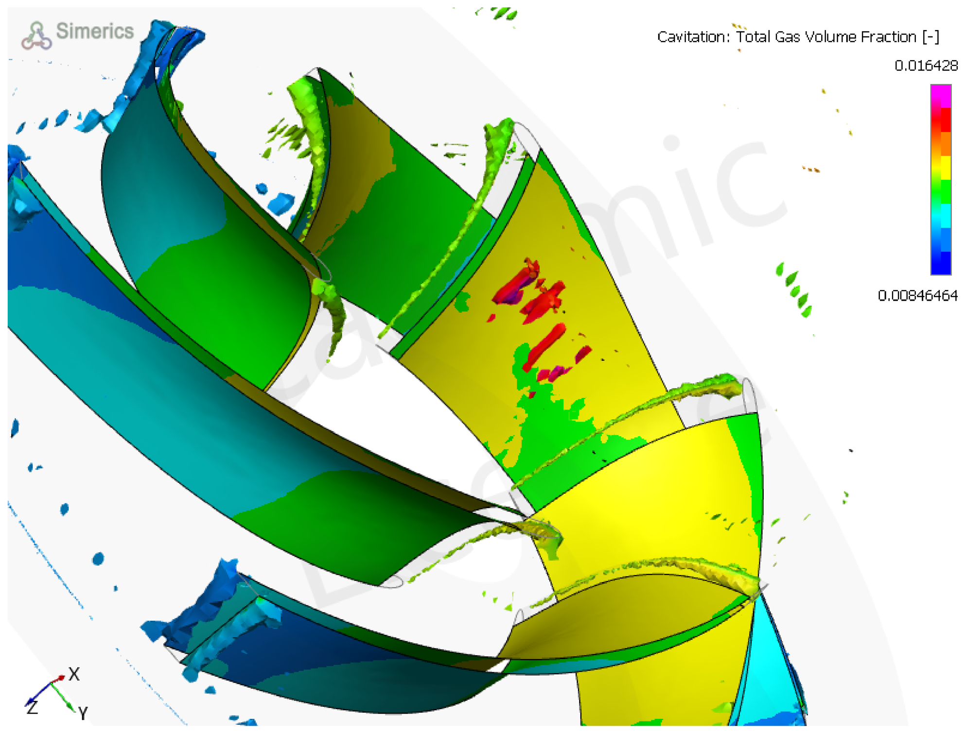
Table A1.
Mesh parameters.
References
- Chitale, S.K.; Jadhav, P.N.; Dhoble, S.S.; Deshmukh, D.M. Parameters Affecting Efficiency of Centrifugal Pump—A Review. Int. J. Sci. Res. Sci. Technol. 2021, 8, 49–58. [Google Scholar] [CrossRef] [Scilit]
- Gall, F.P. The Corrosion of Centrifugal Pumps in Aqueous Environments. In Proceedings of the Pumps Compressors Conference, Beijing, China, 19–22 September 2013. [Google Scholar]
- Tao, R.; Xiao, R.; Wang, F.; Liu, W. Cavitation behavior study in the pump mode of a reversible pump-turbine. Renew. Energy 2018, 125, 655–667. [Google Scholar] [CrossRef] [Scilit]
- Dönmez, A.H.; Yumurtacı, Z.; Kavurmacıoğlu, L. The Effect of Inlet Blade Angle Variation on Cavitation Performance of a Centrifugal Pump: A Parametric Study. J. Fluids Eng. 2019, 141, 4040557. [Google Scholar] [CrossRef] [Scilit]
- Gohil, P.P.; Saini, R.P. Effect of temperature, suction head and flow velocity on cavitation in a Francis turbine of small hydro power plant. Energy 2015, 93, 613–624. [Google Scholar] [CrossRef] [Scilit]
- Bandi, S.; Banka, J.; Kumar, A.; Rai, A.K. Effects of sediment properties on abrasive erosion of a centrifugal pump. Chem. Eng. Sci. 2023, 277, 118873. [Google Scholar] [CrossRef] [Scilit]
- Thapa, B. Sand Erosion in Hydraulic Machinery. PhD Thesis, Norwegian University of Science and Technology (NTNU), Trondheim, Norway, 2004. [Google Scholar]
- Thapa, B.S.; Gjosater, K.; Eltvik, M.; Dahlhaug, O.G.; Thapa, B. Effects of turbine design parameters on sediment erosion of a Francis Turbine runner. In Proceedings of the International Conference on the Developments of Renewable Energy Technology, Dhaka, Bangladesh, 5–7 January 2012. [Google Scholar]
- Finnie, I. Erosion of surfaces by solid particles. Wear 1960, 3, 87–103. [Google Scholar] [CrossRef] [Scilit]
- Wakeman, T.; Tabakoff, W. Measured Particle Rebound Characteristics Useful for Erosion Prediction. In Volume 3: Coal, Biomass and Alternative Fuels; Combustion and Fuels; Oil and Gas Applications; Cycle Innovations; American Society of Mechanical Engineers: New York, NY, USA, 1982. [Google Scholar] [CrossRef] [Scilit]
- Dixon, S.L.; Hall, C.A. Centrifugal Pumps, Fans, and Compressors. In Fluid Mechanics and Thermodynamics of Turbomachinery; Elsevier: Amsterdam, The Netherlands, 2014; pp. 265–317. [Google Scholar] [CrossRef] [Scilit]
- Dixon, S.L.; Hall, C.A. Hydraulic Turbines. In Fluid Mechanics and Thermodynamics of Turbomachinery; Elsevier: Amsterdam, The Netherlands, 2014; pp. 361–418. [Google Scholar] [CrossRef] [Scilit]
- Kan, K.; Binama, M.; Chen, H.; Zheng, Y.; Zhou, D.; Su, W.; Muhirwa, A. Pump as turbine cavitation performance for both conventional and reverse operating modes: A review. Renew. Sustain. Energy Rev. 2022, 168, 112786. [Google Scholar] [CrossRef] [Scilit]
- Mousmoulis, G.; Kassanos, I.; Anagnostopoulos, I. Study and Detection of Cavitation in Centrifugal Pumps. In Cavitation and Bubble Dynamics; Elsevier: Amsterdam, The Netherlands, 2021; pp. 133–171. [Google Scholar] [CrossRef] [Scilit]
- Al-Arabi, A.A.; El-Kadi, M.A. Cavitation in centrifugal pumps handling salted water. J. Eng. Res. Appl. Sci. 2006. [Google Scholar]
- Ceccio, S.; Gowing, S.; Shen, Y.T. The Effects of Salt Water on Bubble Cavitation. J. Fluids Eng. 1997, 119, 155–163. [Google Scholar] [CrossRef] [Scilit]
- Arakeri, V.H.; Acosta, A.J. Viscous Effects in the Inception of Cavitation on Axisymmetric Bodies. J. Fluids Eng. 1973, 95, 519–527. [Google Scholar] [CrossRef] [Scilit]
- Yokoyama, S. Effect of the Tip Shape at Entrance of the Impeller Vane of the Centrifugal Pump on Cavitation. Bull. JSME 1960, 3, 326–332. [Google Scholar] [CrossRef] [Scilit]
- Lu, J.; Li, J.; Zhang, C.; Zhou, Y.; He, Y. Research on the Cavitation Characteristics of Pump Turbines Based on Mode Decomposition. Processes 2025, 13, 732. [Google Scholar] [CrossRef] [Scilit]

Disclaimer/Publisher’s Note: The statements, opinions and data contained in all publications are solely those of the individual author(s) and contributor(s) and not of MDPI and/or the editor(s). MDPI and/or the editor(s) disclaim responsibility for any injury to people or property resulting from any ideas, methods, instructions or products referred to in the content. |
© 2026 by the authors. Licensee MDPI, Basel, Switzerland. This article is an open access article distributed under the terms and conditions of the Creative Commons Attribution (CC BY) license.