


Abstract
Accurate prediction of syngas composition is essential for process design, optimization, and scale-up, yet it remains challenging due to interactions among operating conditions, biomass properties, and chemical reactions. This study used a database of 450 experimental observations spanning a wide range of biomass feedstocks and operating conditions to compare the predictive performance of Aspen Plus simulations and Machine Learning models in estimating the concentrations of CO, CO2, H2, and CH4 in syngas. Aspen Plus was used to simulate the 4 stages of the biomass gasification process under different operating conditions, with special focus on the three reactor modules (RPlug, RGibbs, and REquil) modeling the last two stages. In parallel, Machine Learning models using four regression algorithms (XGBoost, Support Vector Machines, Random Forest and Artificial Neural Networks), with different preprocessing and data-splitting strategies, were evaluated for predicting syngas composition. The best Machine Learning models achieved R2 values of 0.753 (CO), 0.866 (CO2), 0.879 (H2) and 0.734 (CH4) on the test set. These results outperformed the Aspen Plus approach and highlight the potential of Machine Learning models as complementary or alternative tools for modelling biomass gasification. Shapley Additive Explanation analysis identified the most influential input variables, revealing key roles for the steam-to-biomass ratio and the equivalence ratio in predicting syngas composition. This study demonstrates that existing Aspen Plus simulation models require further development to improve performance metrics across a wide range of biomass feedstocks and operating conditions.
1. Introduction
The continuous growth of industry and population has intensified the challenge of meeting rising energy demand. At the same time, concerns about energy accessibility, security, and long-term sustainability remain central to the debate on future energy systems. Traditional and renewable energy sources each present important advantages and drawbacks, and choosing an optimal solution is far from straightforward. Compounding this challenge is the persistent issue of waste management. Integrating waste valorization with energy production can support circular economy strategies, enhance resource efficiency, and reduce both environmental impact and pressure on natural resources [1].
Among renewable energy options, biomass stands out as the only carbon-neutral primary resource capable of supplying renewable transportation fuels while simultaneously enabling reductions in NOx and SOx emissions. It also offers a productive route for converting low-value residues into high-value energy carriers [2]. Biomass can be converted through biochemical or thermochemical routes, with the latter gaining increasing attention in recent decades. Within thermochemical processes, gasification has emerged as a highly promising technology, as it enables the production of synthesis gas (syngas) for downstream biofuel synthesis and typically achieves higher efficiency in power generation compared to traditional biomass-to-energy alternatives [3].
Biomass gasification involves reacting carbon-based feedstocks with an oxidant agent—such as air, steam, or oxygen—to produce a mixture predominantly composed of CO and H2, along with smaller amounts of CO2, CH4, N2, and light hydrocarbons. The overall process proceeds through four stages: Drying, Pyrolysis, Oxidation and Reduction. Drying aims to reduce the biomass’ moisture content to less than 5%. In the next stage (Pyrolysis), the volatile components are vaporized in the absence of oxygen and under the effect of temperature. The third stage occurs in the presence of oxygen once again, as the objectives are the partial combustion of combustible substances—mainly char—present in the gas mixture obtained from Pyrolysis and the generation of energy to sustain the process. In the final stage (Reduction), syngas is formed through reactions between the gases and the unburned char from the Oxidation/Partial Combustion stage. The final composition depends on several factors, including the type of biomass, the gasification technology, and the oxidant agent used (e.g., air, steam, or O2) [4].
The composition of syngas is a key parameter that determines its energy content, combustion characteristics, and suitability for downstream applications such as Fischer–Tropsch synthesis and hydrogen production. However, accurately predicting syngas composition remains challenging due to complex interactions among chemical reactions, thermodynamic equilibria, feedstock properties, and operating conditions. Parameters such as Temperature, Pressure, Equivalence Ratio, Steam-to-Biomass Ratio, moisture content, and biomass composition significantly influence the resulting gas mixture. Consequently, reliable prediction models are essential for gasifier design, optimization, and scale-up [5].
The objective of this study is to evaluate several alternatives for simulating the biomass gasification process using Aspen Plus (AP) and Machine Learning (ML) approaches, and to compare their performance in predicting the final syngas composition.
2. Literature Review
A wide range of studies have explored biomass gasification using AP, leveraging its extensive thermodynamic and modelling capabilities. Doherty et al. applied a restricted equilibrium model using the RGibbs reactor to evaluate the influence of parameters such as temperature, biomass composition, steam to biomass ratio, air–fuel ratio, and oxidant agent temperatures on gasification performance [6]. Similarly, Pala et al. used AP with an RGibbs module to investigate how operating temperature and steam to biomass ratio affect the resulting syngas composition [7]. The versatility of AP has also allowed researchers to study the role of feedstock variability: Mehrpooya et al. evaluated 23 different biomass types using RGibbs-based modelling to quantify their impact on syngas characteristics [8]. Other studies, such as that of Safarian et al., have examined downdraft gasifiers using the REquil module to identify optimal operating strategies for the gasifier performance [9].
Despite its advantages, AP modelling also presents several limitations. Developing accurate models requires significant expertise in chemical reaction mechanisms and thermodynamic property estimation. Furthermore, detailed simulations can be computationally intensive and time-consuming, particularly when large numbers are required for optimization or sensitivity analysis. In addition, simplifications and assumptions—such as equilibrium conditions or simplified reaction networks—are often necessary to make the models tractable, which may reduce predictive performance under certain operating conditions [10].
In recent years, ML techniques have gained increasing attention as alternative or complementary tools for modelling complex chemical and energy systems. ML algorithms can identify patterns and relationships within experimental or simulated datasets without requiring explicit knowledge of the underlying physical mechanisms. By learning from data, ML models can rapidly predict system outputs once trained, making them attractive for applications involving large datasets, real-time monitoring, or optimization tasks [11].
Several authors have investigated the application of ML to improve or complement gasification modelling. Elmaz et al. evaluated four ML regression techniques—polynomial regression, support vector regression, decision tree regression, and multilayer perceptron—to predict key syngas components (CO, CO2, CH4, H2) and the high heating value (HHV) for two biomass types: pinecone and wood pellets [12]. Sakheta et al. explored a hybrid approach in which ML models were used to replace one of the Aspen Plus modules, enabling a comparison between fully mechanistic simulations and an integrated ML-enhanced workflow [13]. More recently, Paudel et al. reported an Artificial Neural Network framework coupled with Particle Swarm Optimization for accurate prediction and optimization of biochar yield, higher heating value and carbon content [14].
However, ML models also present challenges. Their predictive capability strongly depends on the quality and quantity of available training data. When data are limited or do not represent the full operating range, ML models may suffer from poor generalization. Additionally, many ML models are considered “black-box,” meaning their internal decision processes may lack transparency and physical interpretability compared with first-principles simulations. Consequently, the integration and comparison of data-driven approaches with traditional process modelling tools remain an important area of research [15].
A comparative analysis between physics-based process simulators and ML models can provide valuable insights into their respective strengths and limitations. AP models benefit from strong physical foundations and interpretability, while ML models offer computational efficiency and the ability to capture nonlinear relationships directly from data. Understanding how these approaches perform relative to each other in predicting syngas composition is crucial for identifying suitable modelling strategies for biomass gasification systems [16].
Thus, the present study aims to compare the predictive performance of AP simulations and ML models for estimating syngas composition in biomass gasification processes. Specifically, this work investigates how well each modelling approach predicts the concentrations of major syngas components under varying operating conditions. A simulation model for the gasification process was developed in AP using thermodynamic equilibrium and process simulation principles. At the same time, ML algorithms were trained on datasets generated from experimental data. The predictive performance of both approaches was then evaluated and compared.
By systematically assessing these two modelling paradigms, this research contributes to a better understanding of their roles in gasification modelling and process optimization. The results provide insights into whether data-driven methods can complement or potentially replace traditional process simulation tools in certain applications.
The present work differentiates itself from previous contributions by simultaneously evaluating the three AP reactor modules most widely applied in gasification studies for the Oxidation and Reduction stages—RPlug, RGibbs, and REquil—and comparing their predictive performance directly with the performance of ML models.
From the ML perspective, the main differences between this study and previous works lie in the combination of multiple preprocessing techniques and advanced data splitting strategies with various regression algorithms, and in the range of observations used to generate Machine Learning-only models. By doing so, it seeks to ensure more robust model performance across a wide range of biomass feedstocks and operating conditions.
3. Materials and Methods
3.1. Database and Data Preparation
In this work, a database with 450 experimental observations compiled by Sakheta et al. was used to compare the results of AP with ML approaches for predicting syngas composition [13]. This database includes 40 types of biomass, operating temperatures between 600 and 1100 °C, and different combinations of oxidant agents, along with the concentrations of CO, CO2, H2, and CH4 in the syngas. Biomass types are characterized by their proximate and ultimate analysis. The first uses four categories for this purpose—Moisture Content (MC), Fixed Carbon (FC), Volatile Matter (VM) and Ash—while the second is divided according to chemical elements—Carbon (C), Oxygen (O), Nitrogen (N), Sulphur (S) and Hydrogen (H). The type and amount of oxidant agents used are expressed by the Equivalence Ratio (ER) and the Steam-to-Biomass Ratio (S/B). The Equivalence Ratio is the ratio of the amount of air supplied to the amount of air required stoichiometrically for complete combustion (Equation (1)). The Steam-to-Biomass Ratio is the ratio of the amount of steam to the amount of biomass fed into the system (Equation (2)). There is no variable representing the amount of O2 supplied as an oxidant agent because this database does not include the use of concentrated O2 for that purpose. Biomass proximate and ultimate analyses, along with Temperature, ER, and S/B, comprise the 12 input variables used in this study. The 4 output variables considered were the volume percentage (Vol%) of carbon monoxide (CO), carbon dioxide (CO2), hydrogen (H2) and methane (CH4) in syngas.
where is the mass flow rate of steam and is the mass flow rate of biomass fed into the gasification process.
Table 1 provides more detailed information regarding the variable values in the database.
Table 1.
Variables and data range of the dataset.
Preprocessing involved removing observations with missing values, followed by detecting and removing outliers. Outlier detection and removal were carried out using the Covariance matrix, the Mahalanobis distance (Equation (3)), and the Chi-Square distribution [17].
where is the Squared Mahalanobis Distance, is the observation point, is the mean vector of the data distribution and is the data’s covariance matrix. T represents the transpose of the vector (x − μ) and −1 the inverse of the covariance matrix.
For each observation, the Squared Mahalanobis Distance is calculated to quantify its deviation from the multivariate mean and to be compared afterwards with the critical value from the Chi-Square distribution. The critical value of the Chi-Square distribution depends on the selected significance level and on the degrees of freedom. In this study, the significance level was 0.05, and the degrees of freedom were equal to the number of input variables, 12. Each observation’s squared distance is subsequently compared to this threshold: if it exceeds the critical value, the observation is flagged as a potential outlier; otherwise, it is considered consistent with the underlying distribution. Finally, the identified outliers were removed.
In the next step, data were split into training and testing sets, with specific proportions (commonly 75% and 25% for training and testing sets), using Kennard–Stone algorithm (KS), SPXY algorithm and Random Split (RS) [18,19]. RS was performed using the train_test_split function from scikit-learn [20]. The algorithms for KS and SPXY are explained below. Assuming sample matrices like the following:
The formulas for calculating the distance for KS (Equation (4)) and SPXY (Equation (5)) are shown below:
where is the distance for the Kennard–Stone method, and are elements of the matrix.
where is the distance for the SPXY method, and are elements of the matrix, and and are elements of the . The main difference between the two methods is that SPXY takes into consideration the values from the variable .
3.2. Aspen Plus Simulation Process
Aspen Plus V14.0 was used to construct a detailed process simulation model of biomass gasification to estimate syngas composition. This software includes a large property database for chemical components, which is used in calculations. Model development involved selecting system components from the AP databanks, configuring the property method, defining conventional and non-conventional components, and assembling a flowsheet reflecting the four main stages of gasification—using unit operation blocks and connecting material and energy streams, defining feed streams (flow rate, composition) and specifying unit operation blocks (thermodynamic condition, chemical reactions, etc.).
Different conventional components were selected from the database, along with two non-conventional components for biomass and ash modelling. The Peng–Robinson equation of state with the Boston–Mathias alpha function (PR-BM) was adopted to compute thermodynamic properties. Biomass was modelled as a non-conventional solid (MIXCINC stream class), with enthalpy and density estimated via HCOALGEN and DCOALIGT. Proximate, ultimate, and sulfur analyses were used to characterize the biomass feed.
The assumptions considered during the modelling of the gasification process in Aspen Plus are as follows:
- Isothermal and steady state process.
- The pressure drop across the blocks is zero.
- Operation at atmospheric pressure (~1 bar).
- No heat and pressure losses occur in the gasifier.
- Tar formation is not considered.
- Char contains only carbon.
- Ash is inert without catalytic activity.
These assumptions are according to the work of Prins et al., who realized the importance of identifying a suitable departing hypothesis to preserve the predictive capacity of the thermodynamic model [21].
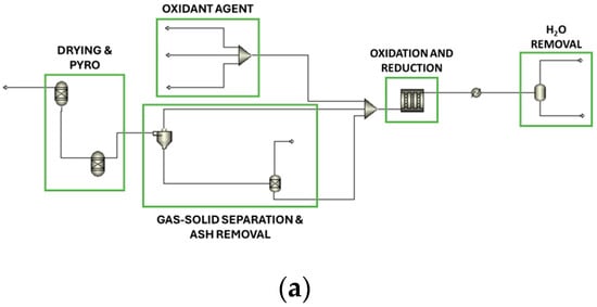
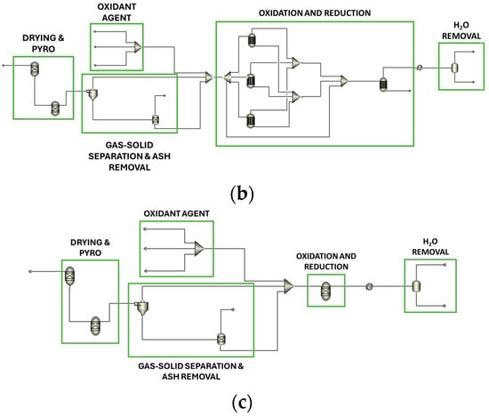
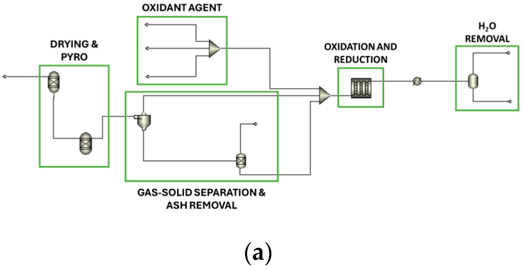
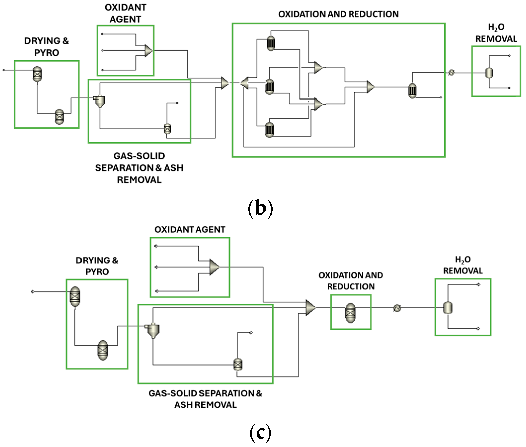
Although gasification occurs in a single reactor in practice, in AP, the process is divided into multiple modules to represent Drying, Pyrolysis, Oxidation and Reduction. Three alternatives were considered, with the primary difference being the Aspen Plus modules used more commonly in the Oxidation and Reduction stages. The Aspen Plus simulation model is shown in Figure 1.
Figure 1.
Aspen Plus simulation model with (a) RPlug, (b) REquil and (c) RGibbs.
In the first section, an RYield block, combined with an RGibbs block, simulates the decomposition of biomass into its elemental constituents and moisture removal. Then, gas–solid separation is performed using an SSplit module to remove solid carbon and ash from the gas stream. Also in this section, solid carbon is separated from the ash in a module called Sep. In the Oxidant Agent section, there are three feed streams—air, concentrated O2, and steam—which are mixed before entering the gasifier models. As mentioned earlier, the database used contains no records involving the use of concentrated O2. Consequently, there are cases where only air is used, others where only steam is used, and others where both air and steam are used simultaneously. After that, the gas stream from the SSplit, the reused solid carbon from Sep, and the oxidant agent are combined into a single stream to be fed to the reactors for the Oxidation and Reduction stages in the same reactor—the reactors are fed without any flow division. For the Oxidation and Reduction stages, the Aspen Plus modules chosen were RGibbs (AP–RG), REquil (AP–REQ) and RPlug (AP–RP). The latter two (AP–REQ and AP–RP) operate on a stoichiometric basis, requiring the chemical reactions involved to be specified. The chemical reactions are presented in Table 2 and Table 3 [22].
Table 2.
Main Gasification Reactions: Heterogeneous Reactions.
Table 3.
Main Gasification Reactions: Homogeneous Reactions.
For RPlug (AP–RP configuration), the reactions considered were: R2, R3, R5, R6, R7, and R9. With REquil (AP–REQ configuration), four modules were used, each with two reactions, since the Aspen Plus module supports only one heterogeneous reaction per unit. Thus, the reaction pairs used were: R1 and R5; R2 and R6; R3 and R7; R4 and R8. The reaction kinetics used in the RPlug model were taken from a book by Basu [23].
After the gasification stage, each stream passes through a heat exchanger where it is cooled to 25 °C and then through a separator to remove any water that may be present in the stream leaving the reactors.
For each reactor configuration in AP, input variables—including biomass composition and operating conditions—were loaded to generate predictions for all observations of the test set.
3.3. Machine Learning Approach
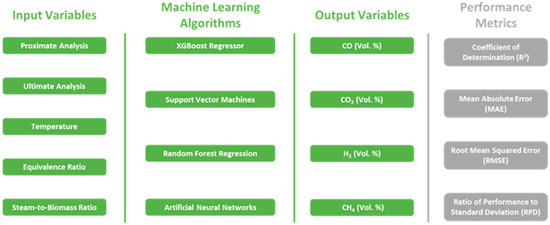
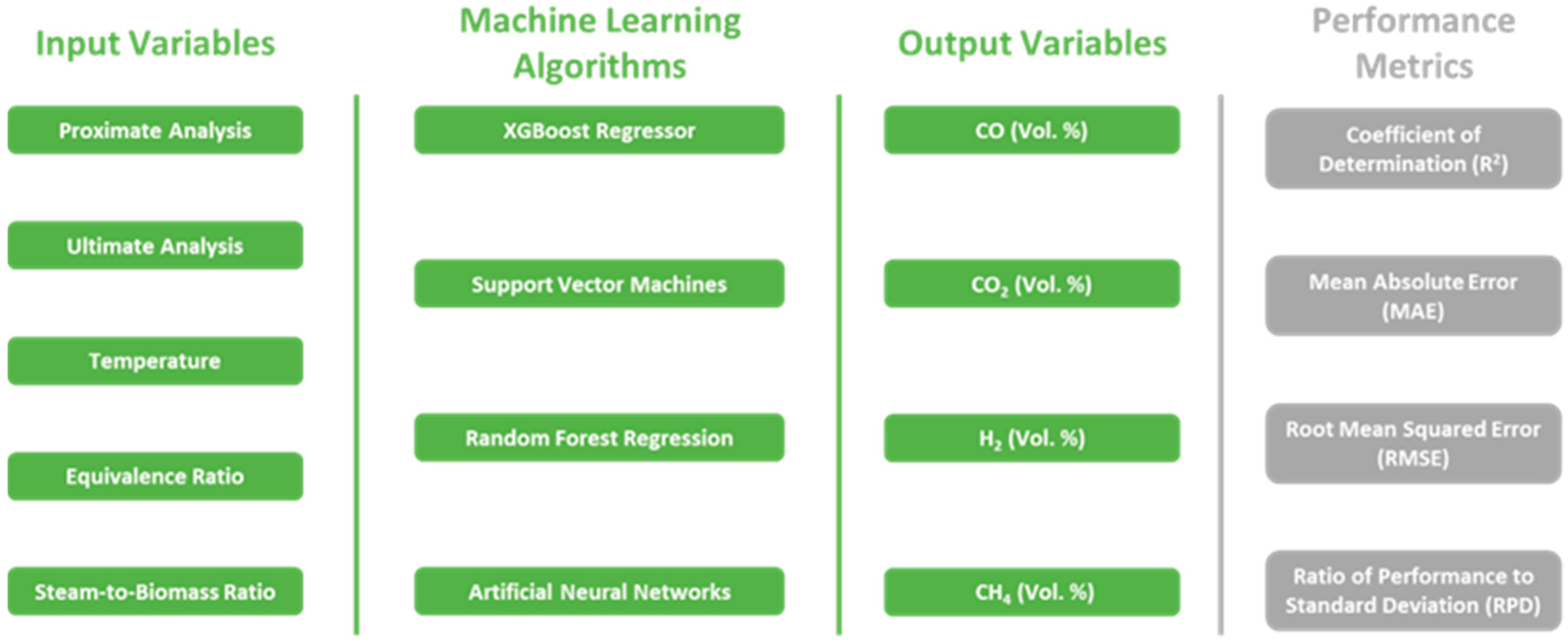
As an alternative to improve predictions of the final composition of syngas, ML models were selected because similar approaches to enhance existing process flowchart simulation models have emerged as a research area of interest, with promising results [16]. With ML, the procedure is to implement a wide range of regression methods and ensure the models developed are suitable for diverse biomass types and operating conditions—ML models simulate the entire process, the four stages of gasification. A diagram summarizing the main variables, algorithms, and evaluation metrics used in this ML approach is shown in Figure 2.
Figure 2.
Summary Diagram for the ML approach.
The results from ML were obtained using software packages supported in Python V3.12, considering the 12 input variables, described in detail in Table 1, for each of the 4 target variables—the compositions of CO, CO2, H2, and CH4 in the syngas, considered individually.
Variable normalization with StandardScaler (SS) was also applied—in some situations optionally, and in others mandatorily, according to the algorithm that would be applied later, before the data was fed into the regression methods. The 4 regression models used were: XGBoost (XGB), Support Vector Machine for Regression (SVR), Random Forest Regression (RFR), and Artificial Neural Network (ANN). The combination of the four regression algorithms, the three data division methods, and the data normalization step yielded 18 models for each property.
To determine the most adequate models, cross-validation (CV) was used, based on the scikit-learn function, with a 5-fold cross-validation strategy [20]. The hyperparameters of each model were optimized using a Python search tool called GridSearchCV. GridSearchCV was used to generate training and test evaluation metrics with values closer to each other, thereby reducing overfitting to the training data. The values of the hyperparameters tested for each model are depicted in Table 4.
Table 4.
Range of values of the hyperparameters tuned for ML models.
The performance of each model was also evaluated through the calculation of the following performance metrics: Coefficient of Determination (R2) (Equation (6)), Mean Absolute Error (MAE) (Equation (7)), Root Mean Squared Error (RMSE) (Equation (8)) and Ratio of Performance to Standard Deviation (RPD) (Equation (9)). These metrics are defined as follows:
where is the number of samples of the calibration set or the prediction set; represents the experimental value of the i-th sample; represents the mean of all the experimental values of the calibration set or the prediction set; represents the predicted value of the i-th sample of the calibration set or the prediction set by the prediction model. Note that it is possible that the R2 of the prediction set calculated could be negative because the prediction formula may perform worse than using the mean of the prediction set being predicted. The model’s performance is better when R2 and RPD are higher, and MAE and RMSE are lower. In the specific case of the RPD, models with values greater than 2.5 are considered sufficient for screening, whereas those with values less than 2.0 are not recommended for prediction [24].
To understand the importance of each input variable and how they influence the output variables, a Shapley Additive Explanation (SHAP) analysis was performed on the predicted results. SHAP analysis is a method used to interpret ML models and to understand how much each variable contributes to a model’s prediction based on the Game Theory method [25]. A positive SHAP value increases the model’s prediction, while a negative SHAP value decreases the prediction. The magnitude of the value indicates the importance of the variable [26].
4. Results and Discussion
Before the data is provided to the simulation models and the ML approach, the database undergoes a preliminary preparation stage, as presented in Section 3.1. After completing the preprocessing steps, during which 36 observations with missing values and 53 outliers were identified and removed, the total number of samples decreased from 450 to 361. These 361 observations were then divided into training and test sets at a 75–25% ratio, as mentioned above, using the 3 methods (RS, SPXY, and KS), leading to a training set of 271 samples and a test set of 90 samples. The training set was used solely for the ML approach to optimize the models and select the best-performing model. The test set was used in both approaches (AP and ML). The final performance of each model is evaluated, and comparisons between them are made based on the test set points.
4.1. Aspen Plus Modelling Results
For the prediction obtained using the AP, simulations were carried out for all points in the test set for each of the four variables. The reactor model with the best performance for predicting each composition was then selected and compared with the best-performing ML model. In this case, the chosen decision metric for comparing the three reactor options was MAE. The values of this metric for the 12 hypotheses—3 reactors × 4 properties—are shown in Table 5. The highlighted cells represent the best performance for each composition.
Table 5.
MAE values for Aspen Plus models.
Based on the MAE values for each reactor, the best options are RGibbs for CO and CO2 and REquil for H2 and CH4. These two reactors will be the options considered in comparison with the ML model.
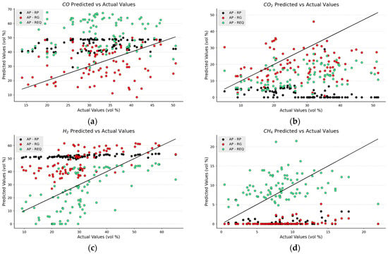
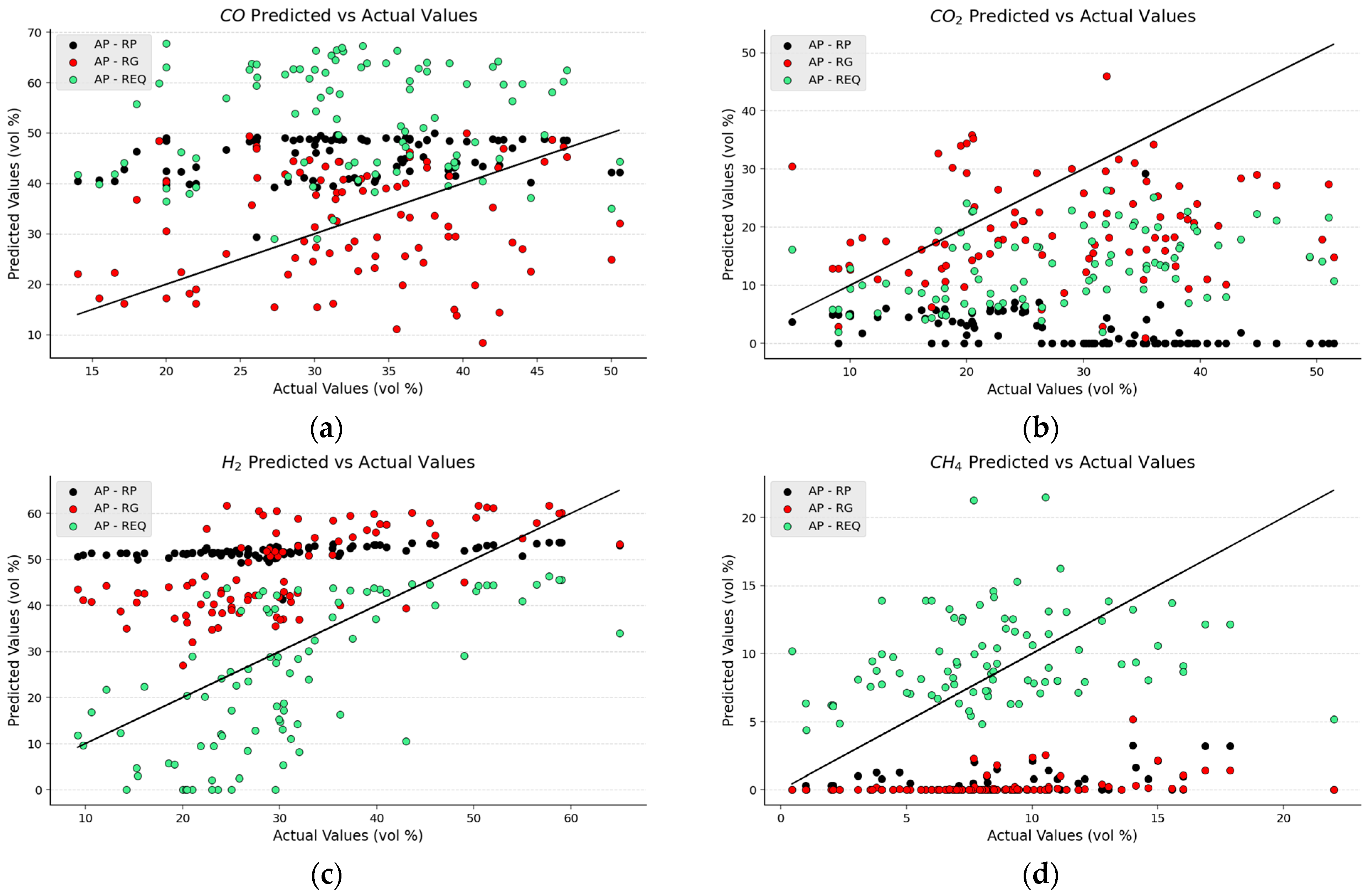
In addition to evaluating the data using a set of metrics to select the best-performing option, plots have been built to understand each reactor’s behavior better and identify explanations for prediction errors. Figure 3 shows the four plots used for the analysis.
Figure 3.
Comparison between testing AP–RP, AP–RG and AP–REQ results for 90 different cases for predicting (a) CO, (b) CO2, (c) H2, and (d) CH4 (Test Set).
Analyzing Figure 3a, one can notice that, for CO prediction, RGibbs performs best, while RPlug and REquil tend to overestimate CO across almost all observations.
For CO2, RGibbs once again performs best because, although the REquil data points are relatively close together, they are almost all below the line x = y, whereas RGibbs’ data points are slightly more scattered.
The opposite occurs with H2: the RGibbs points are mostly on the same side of the line, while those for REquil are more widely distributed.
Lastly, for CH4, both RPlug and RGibbs show very little sensitivity to this output, with predictions remaining almost unchanged across the entire range of experimental values.
RPlug shows poor performance and low sensitivity in predicting the 4 compositions—for CH4, the values are close to zero. In contrast, the other 3 compositions are always close to a specific value, forming a line parallel to the x-axis.
4.2. Machine Learning Results
The initial stages of the ML-based approach are performed using the training sets containing the 271 observations. Table 6 shows an example of all the ML models evaluated and the values of their respective metrics for the training set, in this case for predicting CO composition. The hyperparameter optimization was performed using GridSearchCV, minimizing the average RMSE value (CV_Score in Table 6), calculated through the cross-validation procedure implemented in the Python Scikit-learn package [20]. The highlighted row corresponds to the model selected.
Table 6.
Cross-validation score and performance metrics of CO prediction for the training set.
Table 7 presents the values of the metrics for the selected models used to estimate CO2, H2, and CH4 compositions.
Table 7.
Best CV_Score and performance metrics of CO2, H2 and CH4 prediction for the training set.
4.3. Comparison of Aspen Plus and Machine Learning Results
Once the best-performing models from each approach had been selected, a comparison was conducted to determine which was more accurate. Table 8 sums up the results of this comparison.
Table 8.
Performance metrics for the test set.
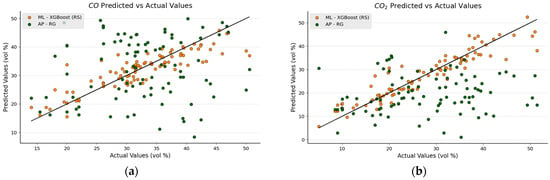
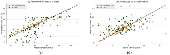
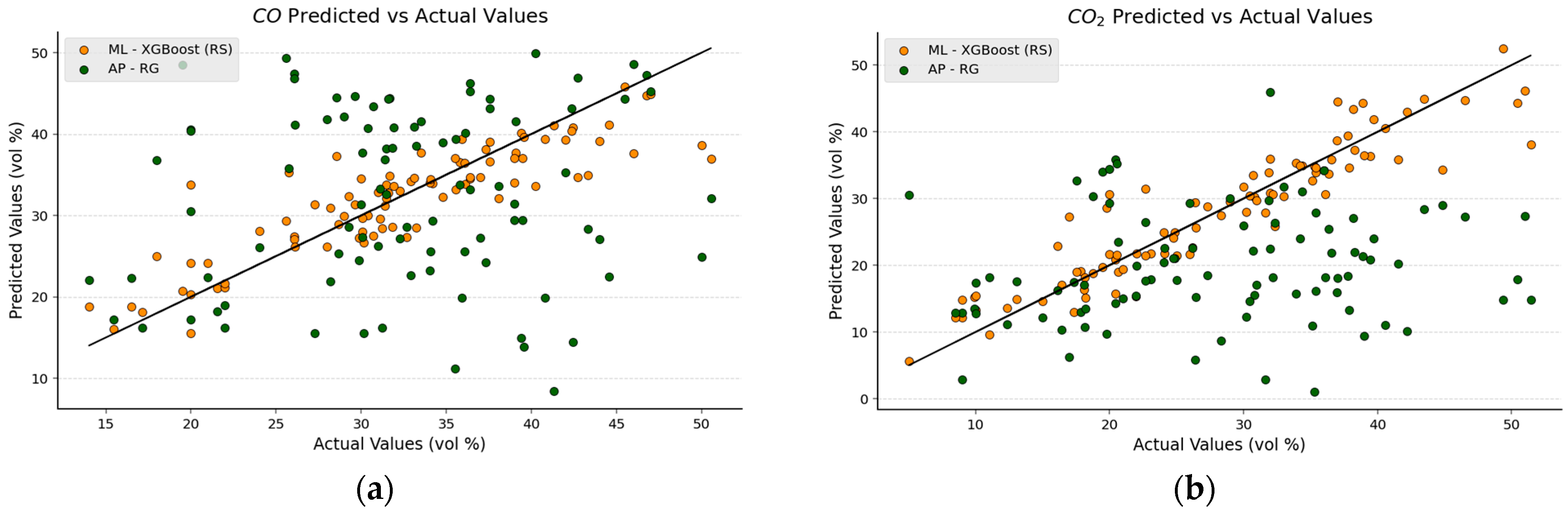
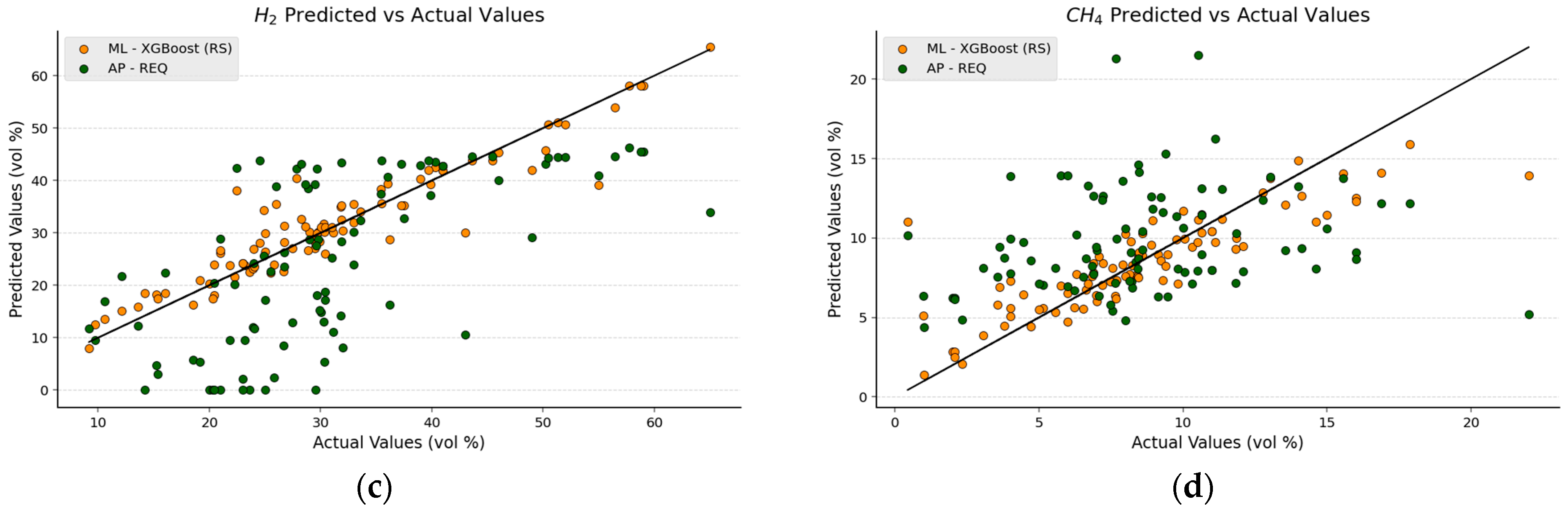
Figure 4 presents the parity plots comparing the predictions of both AP and ML models with the experimental values from the database.
Figure 4.
Comparison between AP and ML results for 90 different cases for predicting (a) CO, (b) CO2, (c) H2, and (d) CH4 (Test Set).
Both the metric values and the figures show that the ML models perform significantly better than the AP ones. The RPD values for the ML models indicate that those are suitable for predicting CO2 and H2, while those for CO and CH4 are close to the limit value (2.0) and still need improvement.
4.4. SHAP Analysis
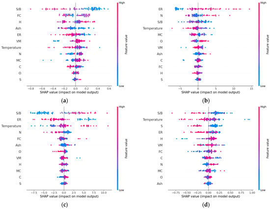
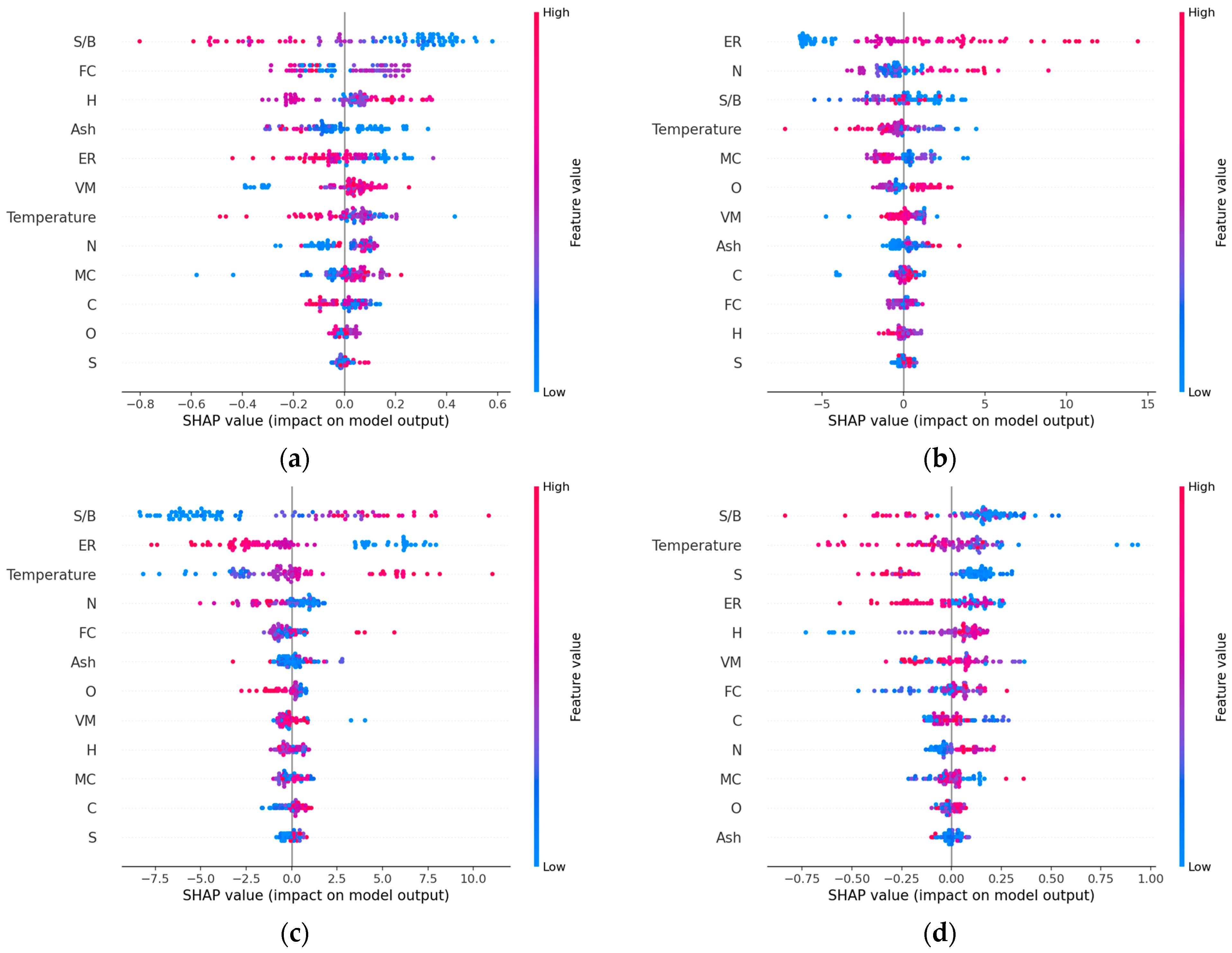
The last stage of the research involved analyzing the importance of each input variable using the SHAP method. This method enables understanding which variables have the greatest influence on the model and how they do so—positively or negatively. The results of the analysis are presented in Figure 5 as summary plots, also known as bee swarm plots.
Figure 5.
Summary plots of the SHAP Analysis cases for (a) CO, (b) CO2, (c) H2, and (d) CH4 (Test Set).
Each point in the plots represents one value of the input variable; therefore, there are as many points for each input as observations are being considered—in this case, 90. This plot provides information such as: which variables have the greatest influence—ranked from most influential to least influential, from top to bottom, on the left-hand side; on the opposite side, there is a color scale for the points on the chart, indicating the dimension of the input value itself—red points represent the observations with the highest values of each feature, and blue points the lowest; the position of the points throughout the plot is directly related to the SHAP value (x-axis) of each point, which translates the individual contribution through the sign of the value—positive or negative—and its magnitude via the absolute value of the SHAP value.
Thus, according to the chosen ML model, the variables with the greatest influence on CO level prediction are the Steam-to-Biomass Ratio (S/B) and Fixed Carbon (FC). S/B carries considerable weight, as the data points are more widely dispersed and further from 0. From the color scale of the points, higher S/B values correspond to lower CO levels, whilst lower S/B values correspond to higher CO levels. There is an inverse relationship between this input and the CO content of the final syngas.
When predicting CO2 levels, the Equivalence Ratio (ER) is the most influential variable. High ER values positively influence the CO2 content of syngas.
In the plot for H2, the discrepancy in the weights of the first 3 variables is no longer as evident—several inputs have many SHAP values far from 0. Temperature, ER and S/B have similar impacts.
The presence of methane in the gasification product depends heavily on S/B and Temperature; the higher these inputs, the lower the CH4 content in the syngas.
5. Conclusions
This study compared the predictive performance of Aspen Plus process simulations and Machine Learning models for estimating the composition of syngas produced during biomass gasification. Three different Aspen Plus reactor modules (RPlug, RGibbs, and REquil) were evaluated for the Oxidation and Reduction stages of the biomass gasification process, and their results were compared with several Machine Learning regression algorithms trained using a diverse dataset of biomass types and operating conditions. The results demonstrate that the predictive performance of the Machine Learning models is significantly better than that of Aspen Plus simulations for all syngas components analyzed.
Among the Aspen Plus models, RGibbs provided the best predictions for CO and CO2, while REquil performed better for H2 and CH4 prediction. However, the overall predictive performance of these models remained limited, with negative R2 values in several cases and RPD values below 1.0 across all outputs.
In contrast, Machine Learning models demonstrated significantly higher predictive performance. The best models achieved R2 values of 0.753 for CO, 0.866 for CO2, 0.879 for H2, and 0.734 for CH4, and RPD values ranged from 1.9 to 2.9.
The Shapley Additive Explanation analysis provided further insights into the influence of input variables on model predictions. The steam-to-biomass ratio and fixed carbon were identified as the most influential variables for CO prediction, while the equivalence ratio had the strongest effect on CO2 formation. For hydrogen production, temperature, equivalence ratio, and steam-to-biomass ratio exerted comparable influences. Methane formation was mainly affected by the steam-to-biomass ratio and temperature.
Overall, the results demonstrate that Machine Learning approaches can significantly outperform conventional thermodynamic simulations in predicting syngas composition. While Aspen Plus models remain valuable for process understanding and mechanistic analysis, Machine Learning models provide faster, more accurate predictions once trained on representative datasets.
Future research using Aspen Plus should focus on improving the representation of complex physical and chemical phenomena, particularly by including tar formation, detailed reaction kinetics, and better modelling of heat and mass transfer limitations. Regarding the Machine Learning approach, using real-time data to monitor the gasification process could expand the existing database and, as a result, improve predictive performance.
Author Contributions
Conceptualization, N.M.O.D. and F.G.M.; methodology, N.M.O.D. and F.G.M.; software, N.M.O.D.; validation, N.M.O.D. and F.G.M.; investigation, N.M.O.D. and F.G.M.; resources, F.G.M.; data curation, N.M.O.D.; writing—original draft preparation, N.M.O.D.; writing—review and editing, N.M.O.D. and F.G.M.; supervision, F.G.M.; project administration, F.G.M.; funding acquisition, F.G.M. All authors have read and agreed to the published version of the manuscript.
Funding
This work received financial support from Agenda “H2Driven Green Agenda”, nr. C644923817-00000037, investment project number. 50, financed by the Recovery and Resilience Plan (PRR) and by the European Union—NextGeneration EU. This work was also supported by national funds through FCT/MECI: LEPABE, UID/00511/2025 (https://doi.org/10.54499/UID/00511/2025) and UID/PRR/00511/2025 (https://doi.org/10.54499/UID/PRR/00511/2025) and ALiCE, LA/P/0045/2020 (https://doi.org/10.54499/LA/P/0045/2020).
Data Availability Statement
The database used in this work is available in the online version at doi:10.1016/j.compchemeng.2024.108834 (Supplementary Materials).
Conflicts of Interest
The authors declare no conflicts of interest.
Abbreviations
The following abbreviations are used in this manuscript:
| AP | Aspen Plus |
| ANN | Artificial Neural Network Algorithm |
| C | Carbon—Biomass Ultimate Analysis |
| CV | Cross-validation |
| ER | Equivalence Ratio |
| FC | Fixed Carbon—Biomass Proximate Analysis |
| HHV | High Heating Value |
| H | Hydrogen—Biomass Ultimate Analysis |
| KS | Kennard-Stone Algorithm |
| ML | Machine Learning |
| MC | Moisture Content—Biomass Proximate Analysis |
| N | Nitrogen—Biomass Ultimate Analysis |
| O | Oxygen—Biomass Ultimate Analysis |
| RFR | Random Forest Regression Algorithm |
| RS | Random Split Method for Data Division |
| REQ | REquil Module from Aspen Plus |
| RG | RGibbs Module from Aspen Plus |
| RP | RPlug Module from Aspen Plus |
| SHAP | Shapley Additive Explanation |
| SPXY | SPXY Algorithm |
| SS | Standard Scaler Method for Standardization |
| S/B | Steam-to-Biomass Ratio |
| S | Sulfur—Biomass Ultimate Analysis |
| SVR | Support Vector Machine for Regression Algorithm |
| VM | Volatile Matter—Biomass Proximate Analysis |
| Vol% | Volume Percentage |
| XGB | XGBoost Regression Algorithm |
| wt% | Weight Percentage |
References
- Bezanty, A. Addressing the Energy Trilemma Through Advanced Gasification. Decarbonisation Technology. February 2024. Available online: https://decarbonisationtechnology.com/article/220/addressing-the-energy-trilemma-through-advanced-gasification (accessed on 15 April 2026).
- Azzone, E.; Morini, M.; Pinelli, M. Development of an Equilibrium Model for the Simulation of Thermochemical Gasification and Application to Agricultural Residues. Renew. Energy 2012, 46, 248–254. [Google Scholar] [CrossRef] [Scilit]
- Safarian, S.; Unnþórsson, R.; Richter, C. A Review of Biomass Gasification Modelling. Renew. Sustain. Energy Rev. 2019, 110, 378–391. [Google Scholar] [CrossRef] [Scilit]
- Basu, P. Combustion and Gasification in Fluidized Beds; Dekker, M., Ed.; CRC Press: Boca Raton, FL, USA, 2004. [Google Scholar]
- Gao, Y.; Wang, M.; Raheem, A.; Wang, F.; Wei, J.; Xu, D.; Song, X.; Bao, W.; Huang, A.; Zhang, S.; et al. Syngas Production from Biomass Gasification: Influences of Feedstock Properties, Reactor Type, and Reaction Parameters. ACS Omega 2023, 8, 31620–31631. [Google Scholar] [CrossRef] [Scilit] [PubMed]
- Doherty, W.; Reynolds, A.; Kennedy, D. Aspen Plus Simulation of Biomass Gasification in a Steam Blown Fluidised Bed; Formatex Research Centre: Norristown, PA, USA, 2013. [Google Scholar]
- Pala, L.P.R.; Wang, Q.; Kolb, G.; Hessel, V. Steam Gasification of Biomass with Subsequent Syngas Adjustment using Shift Reaction for Syngas Production: An Aspen Plus model. Renew. Energy 2017, 101, 484–492. [Google Scholar] [CrossRef] [Scilit]
- Mehrpooya, M.; Khalili, M.; Sharifzadeh, M.M.M. Model Development and Energy and Exergy Analysis of the Biomass Gasification Process. Renew. Sustain. Energy Rev. 2018, 91, 869–887. [Google Scholar] [CrossRef] [Scilit]
- Safarian, S.; Richter, C.; Unnthorsson, R. Waste Biomass Gasification Simulation Using Aspen Plus: Performance Evaluation of Wood Chips, Sawdust and Mixed Paper Wastes. J. Power Energy Eng. 2019, 7, 12–30. [Google Scholar] [CrossRef]
- Loweski Feliz, M.; Abdelouahed, L.; Taouk, B. Comparative and Descriptive Study of Biomass Gasification Simulations Using Aspen Plus. Energies 2024, 17, 4443. [Google Scholar] [CrossRef] [Scilit]
- Xu, Y.; Ge, J.; Ju, C.W. Machine Learning in Energy Chemistry: Introduction, Challenges and Perspectives. Energy Adv. 2023, 2, 896–921. [Google Scholar] [CrossRef] [Scilit]
- Elmaz, F.; Yücel, Ö.; Mutlu, A.Y. Predictive Modeling of Biomass Gasification with Machine Learning-based Regression Methods. Energy 2020, 191, 116541. [Google Scholar] [CrossRef] [Scilit]
- Sakheta, A.; Raj, T.; Nayak, R.; O’Hara, I.; Ramirez, J. Improved Prediction of Biomass Gasification Models through Machine Learning. Comput. Chem. Eng. 2024, 191, 108834. [Google Scholar] [CrossRef] [Scilit]
- Paudel, P.P.; Park, S.; Oh, K.C.; Kim, D.H. Artificial Neural Network Modeling for Prediction and Optimization of Biochar Yield and Properties. J. Anal. Appl. Pyrolysis 2026, 193, 107421. [Google Scholar] [CrossRef] [Scilit]
- Lipton, Z.C. The Mythos of Model Interpretability. ACM Queue 2018, 16, 31–57. [Google Scholar] [CrossRef] [Scilit]
- Jadoon, U.K.; Díaz, I.; Rodríguez, M. A Comparative Study of Aspen Plus and Machine Learning Models for Syngas Prediction in Biomass-Plastic Waste Co-gasification. In Proceedings of the 35th European Symposium on Computer Aided Process Engineering (ESCAPE 35); PSE Press: Notre Dame, IN, USA, 2025; Volume 4, pp. 370–375. [Google Scholar] [CrossRef] [Scilit]
- Leys, C.; Klein, O.; Dominicy, Y.; Ley, C. Detecting Multivariate Outliers: Use a Robust Variant of the Mahalanobis Distance. J. Exp. Soc. Psychol. 2018, 74, 150–156. [Google Scholar] [CrossRef] [Scilit]
- Galvão, R.K.H.; Araujo, M.C.U.; José, G.E.; Pontes, M.J.C.; Silva, E.C.; Saldanha, T.C.B. A Method for Calibration and Validation Subset Partitioning. Talanta 2005, 67, 736–740. [Google Scholar] [CrossRef] [Scilit] [PubMed]
- Kennard, R.W.; Stone, L.A. Computer Aided Design of Experiments. Technometrics 1969, 11, 137–148. [Google Scholar] [CrossRef]
- Scikit-Learn Developers. Scikit-Learn: Machine Learning in Python. Available online: https://scikit-learn.org/stable/ (accessed on 19 March 2026).
- Prins, M.J.; Ptasinski, K.J.; Janssen, F.J.J.G. From Coal to Biomass Gasification: Comparison of Thermodynamic Efficiency. Energy 2007, 32, 1248–1259. [Google Scholar] [CrossRef] [Scilit]
- Puig-Arnavat, M.; Bruno, J.C.; Coronas, A. Review and Analysis of Biomass Gasification Models. Renew. Sustain. Energy Rev. 2010, 14, 2841–2851. [Google Scholar] [CrossRef] [Scilit]
- Basu, P. Biomass Gasification and Pyrolysis: Practical Design and Theory; Academic Press: Cambridge, MA, USA, 2010. [Google Scholar]
- Wang, Y.; Yuan, H.; Xiong, Z. Transfer of Near-infrared Analysis Models for Gasoline RON based on Ensemble Learning. Microchem. J. 2024, 206, 111513. [Google Scholar] [CrossRef] [Scilit]
- Lundberg, S.M.; Allen, P.G.; Lee, S.-I. A Unified Approach to Interpreting Model Predictions. 2017. Available online: https://github.com/slundberg/shap (accessed on 15 April 2026).
- Ponce-Bobadilla, A.V.; Schmitt, V.; Maier, C.S.; Mensing, S.; Stodtmann, S. Practical guide to SHAP analysis: Explaining Supervised Machine Learning Model Predictions in Drug Development. Clin. Transl. Sci. 2024, 17, e70056. [Google Scholar] [CrossRef] [Scilit] [PubMed]

Disclaimer/Publisher’s Note: The statements, opinions and data contained in all publications are solely those of the individual author(s) and contributor(s) and not of MDPI and/or the editor(s). MDPI and/or the editor(s) disclaim responsibility for any injury to people or property resulting from any ideas, methods, instructions or products referred to in the content. |
© 2026 by the authors. Licensee MDPI, Basel, Switzerland. This article is an open access article distributed under the terms and conditions of the Creative Commons Attribution (CC BY) license.