Research on Reliability Evaluation Method of Distribution Network Considering the Temporal Characteristics of Distributed Power Sources

Abstract

Large-scale integration of photovoltaics (PV) introduces complex source-load temporal volatility and grid-connection/off-grid transitions. Traditional static reliability assessments fail to capture these dynamics, resulting in “considerable deviations” in system indices. This paper proposes a reliability evaluation framework that couples temporal source-load trajectories with a multi-stage fault recovery process. Unlike traditional methods that rely on a single static snapshot, the proposed model evaluates the system state across a continuous 5-h restoration window. The novelty lies in the unique integration of a Dynamic Time Warping (DTW)–Kmedoids method to preserve temporal phase-shifts and a multi-stage Mixed-Integer Linear Programming (MILP) model to simulate PV grid-connection transitions throughout this window. By capturing the intra-outage evolution of sources and loads, the framework fundamentally corrects the “considerable deviations” of static assessments. Case studies demonstrate high precision with an error of less than 0.71% and a 20-fold speedup. Crucially, the framework corrects the 22.31% risk underestimation bias inherent in static models by tracking real-time source-load evolution. This confirms that temporal coordination performance is the primary determinant of the reliability ceiling in active distribution networks. The findings reveal that the precise alignment of intermittent generation and fluctuating demand defines the actual operational safety margin, providing a superior quantitative foundation for grid resilience enhancement.

1. Introduction

The large-scale integration of distributed generation (DG) such as wind and photovoltaic (PV) power, coupled with electricity market reforms, has fundamentally transformed the characteristics of distribution networks [1]. However, distributed energy resources (DERs) are constrained by weather, leading to inherent instability and output fluctuations, which poses significant challenges to system operation. Traditional reliability assessment methods for distribution networks exhibit notable deficiencies. They predominantly focus on calculating steady-state indices and often neglect the post-fault restoration process. This limitation renders them inadequate for capturing the dynamic characteristics of active networks with multiple power sources. These methods struggle to accurately characterize the operational behavior following renewable integration, are ineffective in addressing source-network parameter mismatch issues under high penetration rates, and fail to adequately integrate the mutual interactions between fault restoration procedures and renewable energy volatility. Consequently, they fall short of meeting the reliability assessment requirements of modern distribution systems.

1.1. Literature Review

1.1.1. Review of Research Status on Reliability Assessment of Traditional Distribution Networks

International academic research on distribution network reliability assessment focuses on algorithm optimization and the innovation of evaluation systems. Customized paradigms are proposed to address topological diversity, providing theoretical support for such studies. Existing methods are divided into two categories: analytical methods and simulation methods. Analytical methods [2,3,4,5,6,7,8,9] describe network topology through precise mathematical models. One category enumerates failure modes with equipment as the core object. For instance, the Failure Mode and Effects Analysis (FMEA) method described in Ref. [10] is suitable for simple networks but suffers from the combinatorial explosion problem. The modular partitioning algorithm presented in Ref. [11] can enhance the assessment efficiency for multi-feeder systems, yet its effectiveness depends heavily on the degree of network modularization. Another category focuses on load nodes. The affine minimal path method presented in Ref. [12] can quickly determine fault isolation areas. Analytical methods offer high accuracy, but their computational complexity increases exponentially with network scale. Simulation methods [13,14,15,16,17,18], namely Monte Carlo simulation, are divided into sequential and non-sequential types. They are suitable for large-scale, complex networks and can accommodate the modeling of multiple random variables. However, they suffer from drawbacks such as time-consuming sampling and difficulties in integration with planning models. To address the time-consuming nature of these simulations, Ref. [19] proposed an accelerated mechanism based on importance sampling and state classification, significantly improving computational efficiency. In traditional reliability assessment, the calculation of steady-state indices predominantly relies on state enumeration or stochastic sampling [20], which simplifies the post-fault recovery into pre-defined duration parameters. This approach neglects the specific operational logic of fault isolation and network reconfiguration. The underlying reason is that traditional analytical frameworks struggle to integrate complex discrete switching actions into continuous probabilistic models. Consequently, they face difficulties in capturing dynamic power supply capability changes in modern distribution networks with multiple sources and reconfiguration paths. Furthermore, existing methods are mostly based on fixed power profiles, failing to reflect the coupling impact of time-varying source-load fluctuations during the restoration period. However, fault recovery is critical for ensuring power supply continuity. Incorporating its dynamic process into assessment models can significantly enhance evaluation accuracy and provide a solid basis for strategy formulation [21].

1.1.2. A Review of Current Research on Reliability Assessment of Distribution Networks with DG

Traditional assessment methods struggle to adapt to the operational characteristics of modern distribution networks. Their capability to address source-network parameter mismatch issues under high penetration levels is insufficient, and they fail to effectively integrate the mutual interactions between fault restoration procedures and renewable energy volatility. Despite extensive research, scenario generation, time series-based modeling, and restoration optimization with Mixed-Integer Linear Programming (MILP) are predominantly studied in isolation [22]. The main technical challenge and research gap lie in the severe disconnect between stochastic temporal modeling and deterministic physical topology optimization. Existing MILP restoration frameworks almost exclusively rely on static data snapshots at a single instant (e.g., worst-case peak load) [23]. However, when a power outage lasts for several hours, a static snapshot cannot capture hazardous intra-outage dynamic transitions (such as the “duck curve” effect where PV output rapidly vanishes just as evening peak load surges). Separately applying time-series scenario generation without physically embedding its continuous trajectories directly into the dynamic restoration optimization process fails to accurately quantify the true support capability of distributed energy resources during prolonged outages [24].

1.2. The Main Work of This Article

The large-scale integration of distributed PV introduces complex source-load temporal features and intermittent grid-connection behaviors, posing significant challenges to traditional assessment methods that rely on static data snapshots. Since static models fail to capture the dynamic evolution of sources and loads during the restoration window, considerable deviations arise between evaluated indices and actual operational risks. These deviations manifest in two primary ways. First, static models mask temporal mismatches, such as sudden PV drops coinciding with peak loads. This causes a severe underestimation of the Expected Energy Not Supplied (EENS). Second, the omission of continuous physical constraints yields overly optimistic results for the System Average Interruption Duration Index (SAIDI).

To eliminate these deviations and reflect the true reliability of active distribution networks, this paper proposes an assessment framework that couples dynamic temporal trajectories with multi-stage physical optimization. The main work and innovations are focused on two aspects. First, a Dynamic Time Warping (DTW)–Kmedoids-based scenario clustering method is developed, leveraging the non-linear alignment of the DTW algorithm to preserve “severe temporal phase-shift features” typically lost in traditional clustering, thereby providing high-fidelity trajectory inputs. Second, a multi-stage MILP model considering source-load temporal characteristics and PV grid-connection/off-grid features is established. By embedding continuous trajectories into the “isolation-reconfiguration-restoration” sequence via virtual fault flows, the model synergistically optimizes switching logic and islanding transitions under linearized physical constraints. This coupling mechanism bridges the gap between stochastic temporal modeling and deterministic topological optimization, fundamentally correcting the deviations of static assessments and providing a more rigorous benchmark for modern grid planning.

2. Scenario Clustering and Typical Scenario Extraction Using DTW–Kmedoids Accounting for Temporal Correlation of Sources and Loads

2.1. The Theoretical Foundation of Algorithms

Considering the volatility and randomness of PV output as well as the temporal correlation between source and load, a scenario clustering method combining DTW and the Kmedoids algorithm is adopted to process PV scenario data with temporal characteristics. The DTW algorithm is used to measure the similarity of different temporal sequences, addressing the time-axis offset problem caused by weather fluctuations or operation mode switching and accurately aligning sequence features. Subsequently, based on the Kmedoids algorithm, the data is clustered to classify operational modes with similar dynamic characteristics into the same clusters. Actual data points are selected as cluster medoids to enhance robustness against outliers, generating a set of typical temporal source-load scenario sets that provide accurate input for subsequent related analyses.

2.1.1. Theoretical Basis of the Kmedoids Algorithm

The traditional Kmedoids algorithm achieves cluster partitioning of datasets through an iterative optimization strategy, and its core lies in constructing a clustering quality evaluation system based on a cost function. The sum of squared clustering errors is defined as the objective function [25].

$$E={\displaystyle \sum _{j=1}^k{\displaystyle \sum _{x\in C_j}{\left|x-O_j\right|}^2}}$$

(1)

where $x$ denotes a sample in each cluster $C_j$; $O_j$ represents its cluster medoid.

The implementation steps of the algorithm are as follows:

• Initial Medoid Selection: Randomly select k samples from the dataset as initial cluster medoids;
• Sample Assignment Phase: Assign non-medoid samples to the nearest cluster based on Euclidean distance;
• Medoid Update: Within each cluster, select the actual sample that minimizes the total distance as the new medoid;
• Convergence Criterion: Repeat Steps 2 and 3 until the variation in the sum of squared errors (SSE) satisfies the adaptive criterion:

$${\displaystyle \frac{|{\mathrm{SSE}}_t-{\mathrm{SSE}}_{t-1}|}{{\mathrm{SSE}}_0}}<\epsilon$$

(2)

where $SS{E}_t$ and $SS{E}_{t-1}$ are the SSE at the current and previous iterations, $SS{E}_0$ is the initial SSE, and $\epsilon$ is the relative tolerance (set to ${10}^{-4}$). This relative threshold scales automatically with the magnitude of input scenarios, ensuring consistent convergence without manual tuning.

Compared with the K-means algorithm, which uses the mean value to determine the virtual center, the Kmedoids algorithm forces the selection of actual samples as cluster medoids, which can significantly reduce the impact of outliers on the clustering results.

2.1.2. Theoretical Basis of the DTW Algorithm

The DTW algorithm was first proposed by Japanese scholar Itakura, and its core is to construct a temporal alignment model based on the idea of dynamic programming. This algorithm breaks through the limitations of traditional equal-length sequence matching. It is specifically designed for the elastic matching of unequal-length sequences. Furthermore, it exhibits superior robust characteristics in complex scenarios, such as temporal phase shifts and amplitude fluctuations. Empirical studies have shown that the synergistic application of DTW features and machine learning models can significantly improve the comprehensive performance of the models [26]. This temporal feature fusion strategy provides a new solution path for complex pattern recognition problems.

The calculation process of DTW is as follows: The distortion degree between the i-th frame $T_i$ of the test template and the j-th frame $R_j$ of the reference template is denoted as $d\left(i, j\right)$, and let $D\left(i, j\right)$ be the distortion degree when the test template has been matched to the i-th frame and the reference template to the j-th frame. To obtain the final result DTW(m, n), a matrix can be defined where the (i,j)-th position contains $d\left(i, j\right)$ and $DTW\left(i, j\right)$. For the warping path $W=\left\{w1,w2,w3,\dots ,wk\right\}$, we have:

$$\left\{\begin{array}{l}\mathrm{DTW}(m,n)={\displaystyle \sum _{i=1}^k{w}_i}\\ d(m,n)={\displaystyle \sum _{i=1}^k{w}_i}\cdot \mathrm{DTW}(m^i,n^i)\end{array}\right.$$

(3)

In the formula, the constraints of w_i are as follows:

(1)

The warping path satisfies $w_1=\left(1,1\right)$, and $w_k =\left(m,n\right)$;

(2)

For any 1 ≤ i < k, when $w_i = \left(a_i,b_i\right)$ and $w_{i+1} = \left(a_{i+1},b_{i+1}\right)$, we have $a_{i+1}$ ≤ $a_i$ + 1 and $b_{i+1}$ ≤ $b_i$ + 1;

(3)

For any 1 ≤ i < k, when $w_i= \left(a_i,b_i\right)$ and $w_{i+1} =\left(a_{i+1},b_{i+1}\right)$, we have $a_{i+1}$ ≥ $a_i$, $b_{i+1}$ ≥ $b_i$, and $a_i + b_i\ne a_{i+1} + b_{i+1}$.

Based on the above constraints, the state transition equation is derived via the dynamic programming method as follows:

$$\mathrm{DTW}(i,j)=\min \left\{\begin{array}{l}\mathrm{DTW}(i-1,j)+d(i,j)\\ \mathrm{DTW}(i,j-1)+d(i,j)\\ \mathrm{DTW}(i-1,j-1)+2d(i,j)\end{array}\right.$$

(4)

In the formula, DTW denotes the shortest distance obtained from the previously traversed region, and d denotes the distance from the previous coordinate to the current coordinate.

2.1.3. Theoretical Basis of the DTW–Kmedoids Algorithm

The Euclidean distance is replaced with the DTW distance, thus forming a new cost function [27] for evaluating the quality of clustering results based on the DTW distance, which is defined as follows:

$$S={\displaystyle \sum _{j=1}^k{\displaystyle \sum _{x\in C_j}\mathrm{DTW}(x-O_j)}}$$

(5)

where $x$ denotes a sample in each cluster $C_j$, and $O_j$ represents its cluster medoid.

By combining the temporal matching advantage of DTW with the robust characteristic of Kmedoids, a clustering method for the temporal characteristics of PV output is constructed. The specific implementation process is as follows:

(1)

Data Standardization: Perform Z-score normalization on the original power sequences;

(2)

Medoid Initialization: Select the initial medoids using the max-min distance method to improve the representativeness of the initial points;

(3)

Dynamic Distance Calculation: Construct a similarity matrix between samples based on DTW;

(4)

Iterative Optimization: Gradually reduce the value of the total cost function by alternately performing sample assignment and medoid update.

2.2. Determination of the Optimal Number of Clustering Scenarios

In Kmedoids cluster analysis, the rationality of the preset number of clusters (K value) directly affects the quality of pattern partitioning. To avoid the risks of overfitting or underfitting caused by manual empirical intervention, this paper conducts a quantitative evaluation of candidate K values based on the classic Elbow Method [28]. This method determines the optimal number of clusters K by analyzing the relationship between the Within-Cluster Sum of Squares (WSS) corresponding to different numbers of clusters, which is defined as the sum of squared Euclidean distances from all samples to their respective cluster medoids, namely:

$$\mathrm{WSS}(K)={\displaystyle \sum _{k=1}^K{\displaystyle \sum _{x_i\in C_k}{‖x_i-m_k‖}^2}}$$

(6)

where $C_{\mathrm{k}}$ denotes the k-th cluster, ${\mathrm{m}}_{\mathrm{k}}$ represents the intra-cluster medoid, and ${‖x_i-m_k‖}^2$ characterizes the dispersion degree of samples relative to the medoid of their affiliated cluster. By enumerating different candidate numbers of clusters, the corresponding WSS values are calculated, and the K-WSS response curve is plotted. The elbow inflection point in the curve where the rate of decrease in WSS slows down significantly is the optimal number of clusters.

3. A Reliability Assessment Method for Distribution Networks Considering the On-Grid and Off-Grid Characteristics of Distributed Power Sources

This chapter develops a distribution network reliability assessment model based on virtual fault flow, incorporating source-load temporal characteristics and PV grid-connection/off-grid features. Case analysis and scenario clustering are conducted to achieve accurate reliability calculation.

3.1. Model Assumption Conditions

The reliability assessment model of distribution networks is related to network topology, component types, and fault types, and different assumptions will affect the complexity of the model. In addition, potential fault conditions in actual operation are complex, and considering all possible faults will bring great difficulties to model construction. Therefore, to better illustrate the model established in this section, the fault types are simplified and the process of load restoration after faults is explained as follows:

• This study adopts the N-1 contingency criterion, considering only single branch faults. This is a standard assumption in reliability assessment, as the simultaneous occurrence of independent multiple faults is statistically negligible in typical distribution networks [29]. While multiple concurrent changes would increase model complexity, they fall outside the scope of this baseline study.
• A distribution system designed with a meshed structure but operating in a radial mode is considered, where each feeder outlet is equipped with a circuit breaker. When a persistent fault occurs, the relay protection system identifies the faulty branch. It then controls the corresponding circuit breaker to trip. This rapid action isolates the downstream fault area, thereby minimizing the number of affected loads.
• After the switching interruption time, the corresponding switches upstream and downstream of the fault are opened to isolate the fault. The network topology is then reconfigured by operating switches and reclosers. Finally, once the fault is cleared, the system restores power supply after the repair-switching interruption time.
• Linear power flow equations are adopted, and line capacity constraints are implemented based on the piecewise relaxation method.

3.2. Virtual Fault Flow Modeling Mechanism

The optimal recovery problem after a fault is modeled as a multi-stage MILP problem. The mathematical core of this model is the Virtual Fault Current mechanism. It converts complex topological searches into linear power flow constraints. To accurately simulate the complete process of “fault isolation—network reconfiguration—load recovery” after a distribution network fault, the VFF mechanism divides the fault recovery process into two core stages. Among them, the RA stage is used to determine the fault isolation scope. The PF stage optimizes the reconfiguration path to maximize load recovery. This linear modeling method ensures that the recovery strategy can be solved to global optimality within seconds. Meanwhile, the power supply status of each node is described by binary variables. This enables quantitative calculation of power outage duration and scope.

(1)

Fault recovery sequence: Fault trigger → Fault Isolation Stage (RA) → Network Reconfiguration Stage (PF) → Load Restoration → System Reset. These two stages correspond to the action logic of circuit breakers and switches, respectively, ensuring the temporal rationality of fault handling;

(2)

Virtual Fault Flow Types:

① RA Stage (Fault Isolation):

By means of the tripping action of circuit breakers to isolate the fault area, only the on-off status of circuit breakers is considered without involving network topology adjustment, and its core objective is to rapidly define the scope of fault impact.

② PF Stage (Network Reconfiguration):

On the basis of fault isolation, the on-off status of branches is adjusted through switch actions to reconstruct the radial power grid topology, thus realizing the load transfer and restoration in non-fault areas.

(3)

Key Variable Definitions:

$p_{i,t}^{xy}$: Binary variable, Node i is in a power outage state at time t after isolation in the RA Stage due to a fault on branch xy (1 indicates power outage, 0 indicates power supply);

$q_{i,t}^{xy}$: Binary variable, Node i is restored to power supply at time t after reconfiguration in the PF Stage (1 indicates restoration, 0 indicates sustained power outage).

3.3. Objective Function

Taking the minimization of the System Average Interruption Duration Index (SAIDI) as the core objective, this index can comprehensively reflect the impacts of power outage scope, duration and the number of users, and is the core quantitative index for distribution network reliability assessment. The expression of the objective function is as follows:

$$\mathrm{SAIDI}={\displaystyle \frac{{\displaystyle \sum _{i\in {\Psi }^{\mathrm{LN}}}{\mathrm{NC}}_i{\mathrm{CID}}_i}}{{\displaystyle \sum _{i\in {\Psi }^{\mathrm{LN}}}{\mathrm{NC}}_i}}}$$

(7)

${\Psi }^{LN}$ denotes the set of load nodes, covering all user nodes in the system for which power supply reliability needs to be evaluated; $N{C}_i$ is the number of users at Node i, which is used to reflect the impact of power outages at different nodes on the overall system reliability in a weighted manner; $CI{D}_i$ represents the average fault duration at Node i (hours/year), reflecting the power outage risk of a single node during long-term operation, and its calculation depends on the fault recovery process simulated by the virtual fault flow.

Selecting SAIDI as the objective function aims to minimize the overall power outage losses of the system. This is achieved by optimizing the action strategies of circuit breakers and switches after faults. Simultaneously, this optimization strictly accounts for the constraints imposed by the grid-connection and off-grid characteristics of DG during the restoration process.

3.4. Constraint Conditions

(1)

Node Power Balance Constraints

$$P_{i,t}^{xy}=P_i{q}_{i,t}^{xy},\forall i\in {\Psi }^{LN}$$

(8)

$$Q_{i,t}^{xy}=Q_i{q}_{i,t}^{xy},\forall i\in {\Psi }^{LN}$$

(9)

$$P_{i,t}^{xy,PV}=q_{i,t-1}^{xy}P{V}_i^{set}{P}_i^{PV},\forall i\in {\Psi }^{LN}$$

(10)

$$Q_{i,t}^{xy,PV}=q_{i,t-1}^{xy}P{V}_i^{set}{Q}_i^{PV},\forall i\in {\Psi }^{LN}$$

(11)

$$P_{ki,t}^{xy}+P_{i,t}^{xy,PV}={\displaystyle \sum _{j\in {\Psi }_i}{P}_{ij,t}^{xy}+P_{i,t}^{xy},\forall ki\in {\rm Y}}$$

(12)

$$Q_{ki,t}^{xy}+Q_{i,t}^{xy,PV}={\displaystyle \sum _{j\in {\Psi }_i}{Q}_{ij,t}^{xy}+Q_{i,t}^{xy},\forall ki\in {\rm Y}}$$

(13)

$$\begin{array}{c}-\left(2-s_{ij,t}^{i,xy}-s_{ij,t}^{j,xy}\right)M+2\left(r_{ij}{P}_{ij,t}^{xy}+x_{ij}{Q}_{ij,t}^{xy}\right)\le U_{i,t}^{xy}-U_{j,t}^{xy}\\ \le \left(2-s_{ij,t}^{i,xy}-s_{ij,t}^{j,xy}\right)M+2\left(r_{ij}{P}_{ij,t}^{xy}+x_{ij}{Q}_{ij,t}^{xy}\right),\forall ij\in {\rm Y}\end{array}$$

(14)

$$U_{i,t}^{xy}={\left(V^S\right)}^2,\forall i\in {\Psi }^{SS}$$

(15)

$$\underset{¯}{U}\le U_{i,t}^{xy}\le \overline{U},\forall i\in {\Psi }^{LN}$$

(16)

$$P_{PV,\min }\le P_{i,t}^{xy,PV}\le P_{PV,\max }$$

(17)

$$Q_{PV,\min }\le Q_{i,t}^{xy,PV}\le Q_{PV,\max }$$

(18)

This set of constraints ensures the real-time equilibrium of active and reactive power at each node. Equations (8)–(14) implement the linearized DistFlow branch power flow [30] to model the power distribution from the main grid and PV units to the loads. Equations (15) and (16) enforce nodal voltage security boundaries to ensure power quality, while Equations (17) and (18) restrict PV active and reactive outputs within their respective installed capacities and operational limits.

$q_{i,t}^{xy}$: The power supply status of node i when a fault occurs in the xy branch at time t.

$P_{i,t}^{xy}$/$Q_{i,t}^{xy}$: The active/reactive power of node i when a fault occurs in the xy branch at time t.

$P_{i,t}^{xy,PV}$/$Q_{i,t}^{xy,PV}$: The PV active/reactive power at node i when a fault occurs in the xy branch at time t.

$P{V}_i^{set}$: The installation status of PV systems at Node i.

$s_{ij,t}^{i,xy}$/$s_{ij,t}^{j,xy}$: The closure status of the i/j terminal switch of branch ij when the xy branch fails at time t.

$r_{ij}$/$x_{ij}$: The resistance/reactance of branch ij.

$U_{i,t}^{xy}$: The square value of the voltage at node i when a fault occurs in the xy branch at time t.

$M$: Constants used for logical constraints in the large M method.

(2)

Branch Power Flow Capacity Constraints

$$-M{s}_{ij,t}^{j,xy}\le P_{ij,t}^{xy}\le M{s}_{ij,t}^{j,xy},\forall ij\in {\rm Y}$$

(19)

$$-M{s}_{ij,t}^{j,xy}\le Q_{ij,t}^{xy}\le M{s}_{ij,t}^{j,xy},\forall ij\in {\rm Y}$$

(20)

$$-S_{ij}^C\le P_{ij,t}^{xy}\le S_{ij}^C,\forall ij\in {\rm Y}$$

(21)

$$-S_{ij}^C\le Q_{ij,t}^{xy}\le S_{ij}^C,\forall ij\in {\rm Y}$$

(22)

$$-\sqrt{2}{S}_{ij}^C\le P_{ij,t}^{xy}\pm Q_{ij,t}^{xy}\le \sqrt{2}{S}_{ij}^C,\forall ij\in {\rm Y}$$

(23)

$$P_{f,t}^{xy}=P_{t{r}^f,t}^{xy},\forall f\in {\Psi }^F,t{r}^f\in {\rm Y}$$

(24)

$$Q_{f,t}^{xy}=Q_{t{r}^f,t}^{xy},\forall f\in {\Psi }^F,t{r}^f\in {\rm Y}$$

(25)

$$P_{f,t}^{xy}\le S_f^C,\forall f\in {\Psi }^F$$

(26)

$$Q_{f,t}^{xy}\le S_f^C,\forall f\in {\Psi }^F$$

(27)

$$\pm Q_{f,t}^{xy}+P_{f,t}^{xy}\le \sqrt{2}{S}_f^C,\forall f\in {\Psi }^F$$

(28)

Equations (19) and (20) establish the logical coupling between the power flow of branch $ij$ and its switching status under fault scenarios. These constraints ensure that power flow exists if and only if the branch is in a conducting state ($s_{ij}^{xy,t}=1$); otherwise, the active and reactive power flows are forced to zero using the Big-M method. Equations (21)–(28) define the branch capacity limits to prevent thermal overloads during the restoration process. To ensure the computational efficiency of the MILP framework, the original non-linear apparent power constraint is transformed into a set of linear inequalities through the piecewise relaxation method.

$S_{ij}^C$: the apparent power of branch ij.

$P_{t{r}^f,t}^{xy}$/$Q_{t{r}^f,t}^{xy}$: The active/reactive power provided by the transformer.

$P_{f,t}^{xy}$/$Q_{f,t}^{xy}$: The active/reactive power at the outlet of the transformer feeder.

(3)

Network Topology and Islanding Operation Constraints

$$s_{ij,t}^{i,xy}+s_{ij,t}^{j,xy}-1\le l_{ij,t}^{xy}\le \left(s_{ij,t}^{i,xy}+s_{ij,t}^{j,xy}\right)/2,\forall ij\in {\rm Y}$$

(29)

$${\displaystyle \sum _{i\in {\Psi }^{LN}}{q}_{i,t}^{xy}={\displaystyle \sum _{ij\in {\rm Y}}{l}_{ij,t}^{xy}}}$$

(30)

$${\displaystyle \sum _{\forall jk\in {\rm Y}}{k}_{jk,t}^{xy}}-{\displaystyle \sum _{\forall ij\in {\rm Y}}{k}_{ij,t}^{xy}}=K_i,\forall i\in {\Psi }^{LN}$$

(31)

$$K_i=\left\{\begin{array}{l}1, \forall i\in {\Psi }^{PV}\\ 0, \forall i\notin {\Psi }^{PV}\cup {\Psi }^{SS}\end{array}\right.$$

(32)

$$\left|k_{ij,t}^{xy}\right|\le n_{PV}{l}_{ij,t}^{xy},\forall ij\in {\rm Y}$$

(33)

Equations (29) and (30) maintain the radial operational structure of the distribution network, which is a prerequisite for standard protection coordination. To address safety requirements and simplify the control logic, Equations (31)–(33) employ a virtual load and virtual power flow mechanism to suppress unintentional islanding—a design necessity considering that the studied feeders lack dedicated grid-forming inverters capable of independent frequency and voltage regulation during autonomous operation. The grid-connection and off-grid logic of PV units are strictly coupled with their Low Voltage Ride Through (LVRT) capability and protection protocols. This coupling ensures the physical rigor of the reliability assessment. During the immediate post-fault period, the nodal voltage may drop below the safety threshold defined by regional grid codes. If this occurs, the PV unit is mandated to trip (go off-grid). This action prevents equipment damage and satisfies anti-islanding protection requirements. Furthermore, it avoids feeding fault currents, which simplifies the protection coordination for sectionalizing switches. In the restoration phase, the PV status transitions based on the system’s re-energization status. A PV unit re-synchronizes with the grid only after the node is re-connected to the main substation via tie-line operations. Once connected, the PV unit provides active power to reduce the EENS. Simultaneously, it utilizes its inverter’s reactive power capacity to provide voltage support. This dual contribution ensures the feasibility of long-distance load transfer. Consequently, the power supply status $q_{i,t}^{xy}$ depends not only on topological path availability but also on the PV’s ability to maintain localized power quality within the multi-stage optimization framework.

$l_{ij,t}^{xy}$: The connection status of the ij branch when the xy branch fails at time t.

$K_i$: The virtual load of each distributed generator.

$k_{ij,t}^{xy}$: The virtual power associated with the branch

(4)

Switchgear Operation Logic Constraints

$$b_{ij,t}^{i,xy}\ge 1-x_{ij}^{i,CB},\forall ij\in {\rm Y}$$

(34)

$$b_{ij,t}^{j,xy}\ge 1-x_{ij}^{j,CB},\forall ij\in {\rm Y}$$

(35)

$$s_{ij,t}^{i,xy}\ge 1-x_{ij}^{i,SW},\forall ij\in {\rm Y}$$

(36)

$$s_{ij,t}^{j,xy}\ge 1-x_{ij}^{j,SW},\forall ij\in {\rm Y}$$

(37)

$$s_{ij,t+1}^{i,xy}\ge s_{ij,t}^{i,xy},\forall ij\in {\rm Y}$$

(38)

$$s_{ij,t+1}^{j,xy}\ge s_{ij,t}^{j,xy},\forall ij\in {\rm Y}$$

(39)

$$q_{ij,t+1}^{xy}\ge q_{ij,t}^{xy},\forall ij\in {\rm Y}$$

(40)

These constraints synchronize the physical configuration of devices with their operational states. Equations (34)–(37) specify that the action of circuit breakers and switches is strictly governed by their physical installation at specific branch terminals. Equations (38)–(40) describe the “memory effect,” ensuring that devices unaffected by the fault or isolation logic retain their initial operational status.

$b_{ij,t}^{i,xy}$: The operating state of the circuit breaker at terminal i of the ij branch when there is a fault in the xy branch at time t.

$x_{ij}^{i,CB}$/$x_{ij}^{i,SW}$: Installation status of circuit breaker/switch at end i of ij branch.

(5)

Virtual Fault Flow Propagation Constraints

$$f_{xy,t}^{xy,RA}=0$$

(41)

$$-\left(2-b_{ij,t}^{i,xy}-s_{ij}^{i,NO}\right)M+f_{i,t}^{xy,RA}\le f_{ij,t}^{xy,RA}\le \left(2-b_{ij,t}^{i,xy}-s_{ij}^{i,NO}\right)M+f_{i,t}^{xy,RA},\forall ij\in {\rm Y}$$

(42)

$$-\left(2-b_{ij,t}^{j,xy}-s_{ij}^{j,NO}\right)M+f_{j,t}^{xy,RA}\le f_{ij,t}^{xy,RA}\le \left(2-b_{ij,t}^{j,xy}-s_{ij}^{j,NO}\right)M+f_{j,t}^{xy,RA},\forall ij\in {\rm Y}$$

(43)

$${\displaystyle \sum _{ij\in {{\rm Y}}_I^B}{b}_{ij}^{i,NO}}+{\displaystyle \sum _{ij\in {{\rm Y}}_J^B}{b}_{ij}^{j,NO}}-1={\displaystyle \sum _{ij\in {{\rm Y}}_I^B}{b}_{ij,t}^{i,xy}+{\displaystyle \sum _{ij\in {{\rm Y}}_J^B}{b}_{ij,t}^{j,xy}}}$$

(44)

$$0\le f_{i,t}^{xy,RA}\le 1,\forall i\in {\Psi }^{LN}$$

(45)

$$0\le f_{ij,t}^{xy,RA}\le 1,\forall ij\in {\rm Y}$$

(46)

$$f_{i,t}^{xy,RA}=1,\forall i\in {\Psi }^{SS}$$

(47)

$$p_{i,t}^{xy}=1-f_{i,t}^{xy,RA},\forall i\in {\Psi }^{LN}$$

(48)

$$f_{xy,t}^{xy,PF}=0$$

(49)

$$-\left(1-s_{ij,t}^{i,xy}\right)M+f_{i,t}^{xy,PF}\le f_{ij,t}^{xy,PF}\le \left(1-s_{ij,t}^{i,xy}\right)M+f_{i,t}^{xy,PF},\forall ij\in {\rm Y}$$

(50)

$$-\left(1-s_{ij,t}^{j,xy}\right)M+f_{j,t}^{xy,PF}\le f_{ij,t}^{xy,PF}\le \left(1-s_{ij,t}^{j,xy}\right)M+f_{j,t}^{xy,PF},\forall ij\in {\rm Y}$$

(51)

$$0\le f_{i,t}^{xy,PF}\le 1,\forall i\in {\Psi }^{LN}$$

(52)

$$0\le f_{ij,t}^{xy,PF}\le 1,\forall ij\in {\rm Y}$$

(53)

$$f_{i,t}^{xy,PF}=1,\forall i\in {\Psi }^{SS}$$

(54)

$$q_{i,t}^{xy}=f_{i,t}^{xy,PF},\forall i\in {\Psi }^{LN}$$

(55)

$$1-p_{i,t}^{xy}\le q_{i,t}^{xy},\forall i\in {\Psi }^{LN}$$

(56)

Equations (41)–(56) model the network response after a fault. We formulated these constraints by extending the VFF mechanism introduced in Ref. [5]. Specifically, Equations (41)–(48) simulate the Fault Isolation Stage (RA), where the propagation of virtual fault signals identifies the immediate outage area. Equations (49)–(56) model the Network Reconfiguration Stage (PF), simulating the optimal load transfer and restoration via switch actions.

$f_{xy,t}^{xy,RA}$/$f_{xy,t}^{xy,PF}$: The virtual fault flow of the xy branch in the RA/PF stage when a fault occurs in the xy branch at time t.

$p_{i,t}^{xy}$: The power supply status of node i when a fault occurs in the xy branch at time t.

$s_{ij}^{j,NO}$/$b_{ij}^{i,NO}$: In the normal operating state, the switch/circuit breaker at end i of the ij branch is in action.

(6)

Definition of Reliability Indices

$${\mathrm{CID}}_i={\displaystyle \sum _{t=1}^T{\displaystyle \sum _{xy\in {\rm Y}}{\lambda }_{xy}{\tau }_{xy}^{SW}{p}_{i,t}^{xy}}}+{\displaystyle \sum _{t=1}^T{\displaystyle \sum _{xy\in {\rm Y}}{\lambda }_{xy}\left({\tau }_{xy}^{RP}-{\tau }_{xy}^{SW}\right)\left(1-q_{i,t}^{xy}\right)}},\forall i\in {\Psi }^{LN}$$

(57)

$${\mathrm{CIF}}_i={\displaystyle \sum _{t=1}^T{\displaystyle \sum _{xy\in {\rm Y}}{\lambda }_{xy}{p}_{i,t}^{xy}}},\forall i\in {\Psi }^{LN}$$

(58)

$$\mathrm{SAIDI}={\displaystyle \frac{{\displaystyle {\sum }_{i\in {\Psi }^{\mathrm{LN}}}{\mathrm{NC}}_i{\mathrm{CID}}_i}}{{\displaystyle {\sum }_{i\in {\Psi }^{\mathrm{LN}}}{\mathrm{NC}}_i}}}$$

(59)

$$\mathrm{SAIFI}={\displaystyle \frac{{\displaystyle {\sum }_{i\in {\Psi }^{\mathrm{LN}}}{\mathrm{NC}}_i{\mathrm{CIF}}_i}}{{\displaystyle {\sum }_{i\in {\Psi }^{\mathrm{LN}}}{\mathrm{NC}}_i}}}$$

(60)

$$\mathrm{ASAI}=1-{\displaystyle \frac{\mathrm{SAIDI}}{8760}}$$

(61)

$$\mathrm{EENS}={\displaystyle \sum _{h\in \mathrm{H}}\frac{\Delta h}{8760}{\displaystyle \sum _{i\in {\Psi }^{\mathrm{LN}}}{\mathrm{CID}}_i{\mu }_h{L}_i}}$$

(62)

Finally, the binary status variables are converted into quantifiable reliability metrics. Equations (57)–(58) define the Customer Interruption Duration (CID) and Frequency (CIF) for individual load nodes. Equations (59)–(62) aggregate these into system-level indices, including SAIDI, System Average Interruption Frequency Index (SAIFI), Average Service Availability Index (ASAI), and EENS.

${\lambda }_{xy}$: Failure rate of branch roads.

${\tau }_{xy}^{SW}$: Switching interrupt time.

${\tau }_{xy}^{RP}$: Repair-switching interruption time.

4. Case Study Analysis

4.1. Experimental Environment

To ensure the reproducibility of the proposed methodology, the experimental environment is specified as follows. All simulations, including the DTW-based scenario clustering and the reliability assessment of the distribution network, were conducted on a high-performance computing platform. The hardware configuration includes an AMD Ryzen 7 5800H processor (3.20 GHz) and 16 GB of RAM. On the software side, the entire algorithmic framework was implemented using the MATLAB R2022a programming environment. Specifically, the MILP models for virtual fault flow and optimal network reconfiguration were formulated using the YALMIP 20210331 optimization toolbox and solved to optimality using the IBM ILOG CPLEX solver was developed by IBM, located in Armonk, NY, USA. This configuration provides a stable and consistent environment for verifying the computational efficiency and accuracy of the results presented in this case study.

4.2. Test System Description

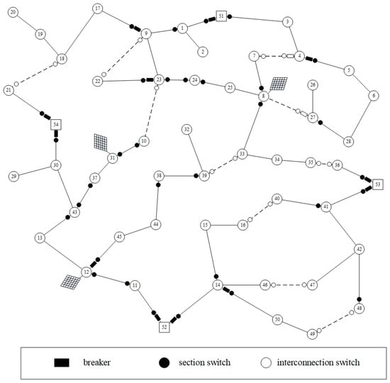
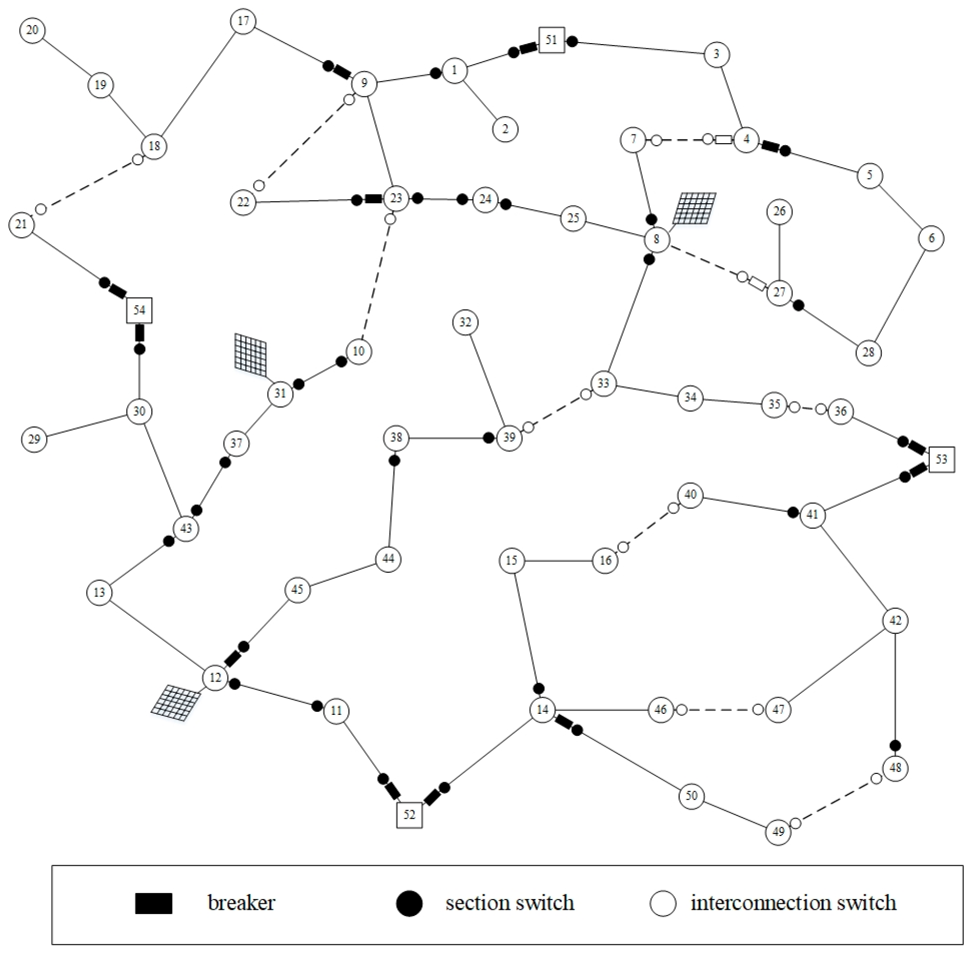
To verify the feasibility of the established model and method, a 54-bus distribution system as shown in Figure 1 is adopted as a case study [31]. The 54-bus distribution system is deliberately adopted as the testbed because its topological characteristics perfectly align with the core objectives of this study. A primary focus of our proposed methodology is to evaluate complex cross-substation load transfer capabilities and collaborative fault restoration. To effectively verify this, the testbed must feature a multi-substation structure interconnected by flexible tie-lines. The 54-bus system perfectly provides this environment, demonstrating how our MILP model optimizes multi-source power routing during emergencies. In contrast, standard single-source radial benchmarks (e.g., the IEEE 33-bus system) completely lack the inter-substation collaboration capability required for our analysis. Furthermore, transmission-level benchmarks like the IEEE 118-bus system are fundamentally unsuitable, as they do not reflect the specific operational constraints of distribution networks. This system consists of 50 load nodes, 4 substation nodes, 8 feeders, and 61 branches. The system base power is 1 MVA, and the base voltage is 13.5 kV; the failure rate of all branches is 0.1 times per (kilometer · year); the system’s repair-switching interruption time ${\tau }_{xy}^{RP}$ and switching interruption time ${\tau }_{xy}^{SW}$ are set to 3 h and 0.5 h, respectively. Three load conditions are considered, with their coefficients being 70% (2000 h/year), 83% (5760 h/year), and 100% (1000 h/year) of the peak demand corresponding to each load condition. Nodes 8, 12, and 31 in the system are selected as PV connection points, with a total installed PV capacity of 2000 kWp.

Figure 1. Topology of 54-Node Distribution System.

4.3. Extraction of Typical Scenarios of Source and Loads

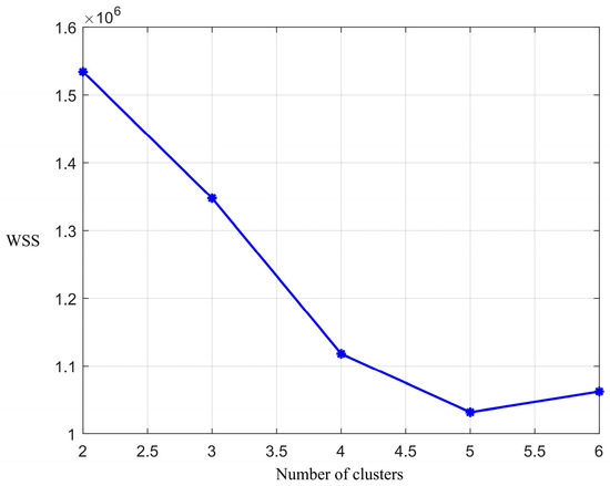
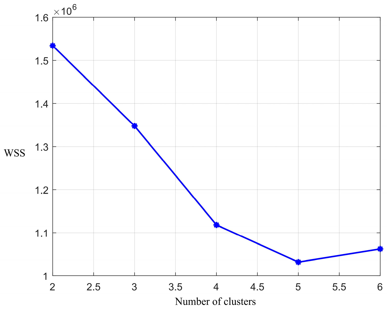
The simulation dataset comprises a full year (8760 h) of historical load demand and photovoltaic (PV) grid-connected output data from the urban distribution network in the Jiaxing Economic and Technological Development Zone, provided by the local utility company. Given that a typical fault recovery process generally does not exceed 5 h, temporal data segments of this length are extracted for the dynamic analysis. Specifically, the data is sampled at 15 min intervals, yielding 20 discrete sampling points for each 5-h restoration window. The Within-Cluster Sum of Squares (WSS) values for different numbers of clusters are calculated using the classic Elbow Method to quantitatively evaluate candidate cluster numbers. By analyzing the active and reactive power, the optimal number of clustering scenarios is determined. To determine the optimal number of scenarios, the Within-Cluster Sum of Squares (WSS) was calculated for candidate cluster numbers ranging from 2 to 6, as illustrated in Figure 2. The results show a sharp reduction in WSS when $K$ increases from 2 to 4, indicating significant improvements in clustering density. At $K=5$, the WSS curve reaches a distinct “elbow” point, where the rate of decrease diminishes significantly. Statistically, $K=5$ represents the threshold where further increasing the cluster count offers marginal accuracy gains while unnecessarily complicating the subsequent MILP optimization. From a physical perspective, these five clusters accurately categorize the primary diurnal power profiles—ranging from winter heating peaks to summer cooling transitions—ensuring the reliability assessment covers both typical and high-risk operational states.

Figure 2. WSS Values with Different Cluster Numbers.

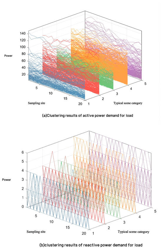
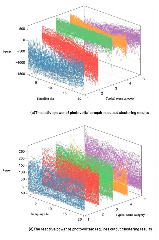
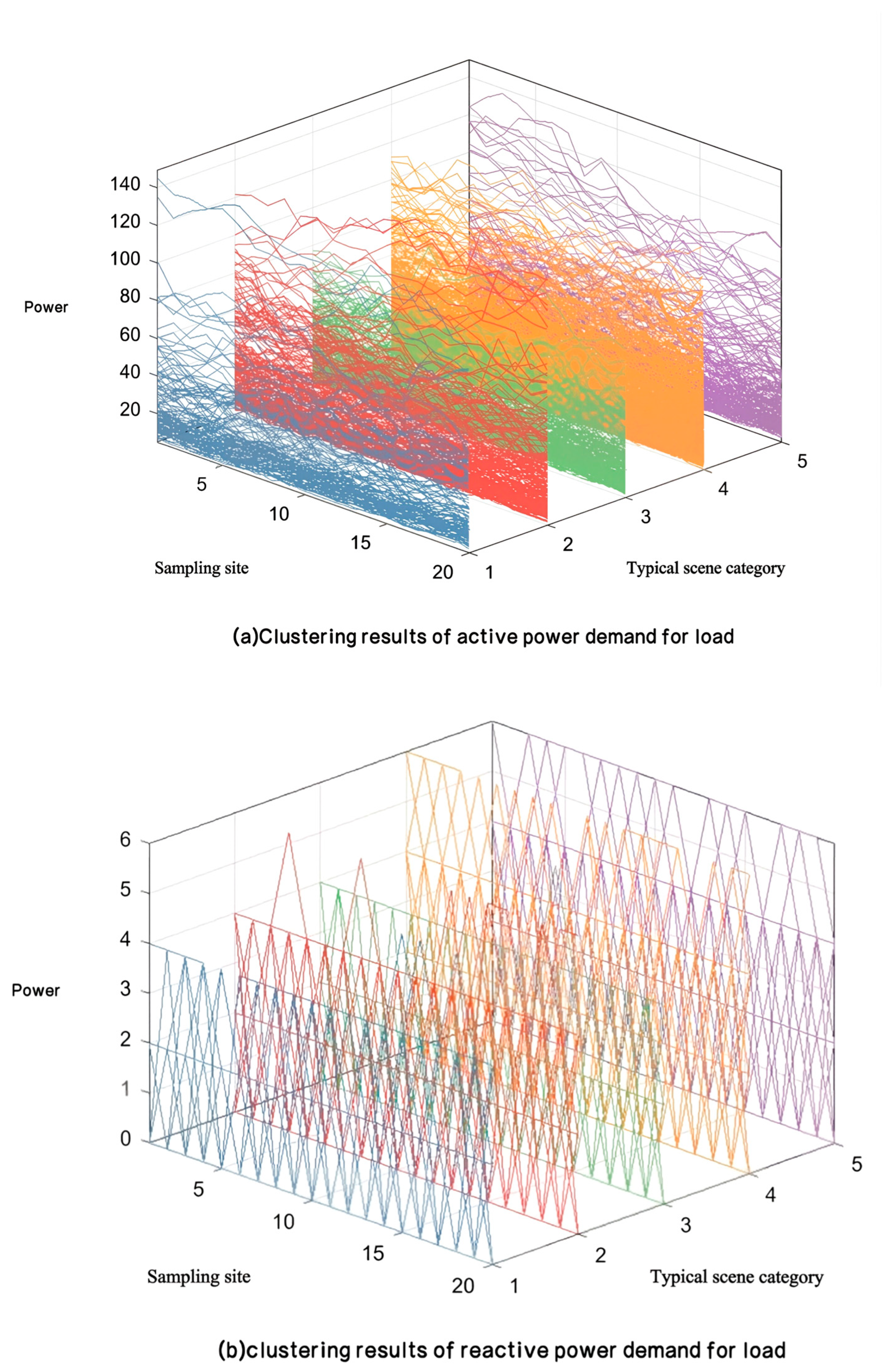
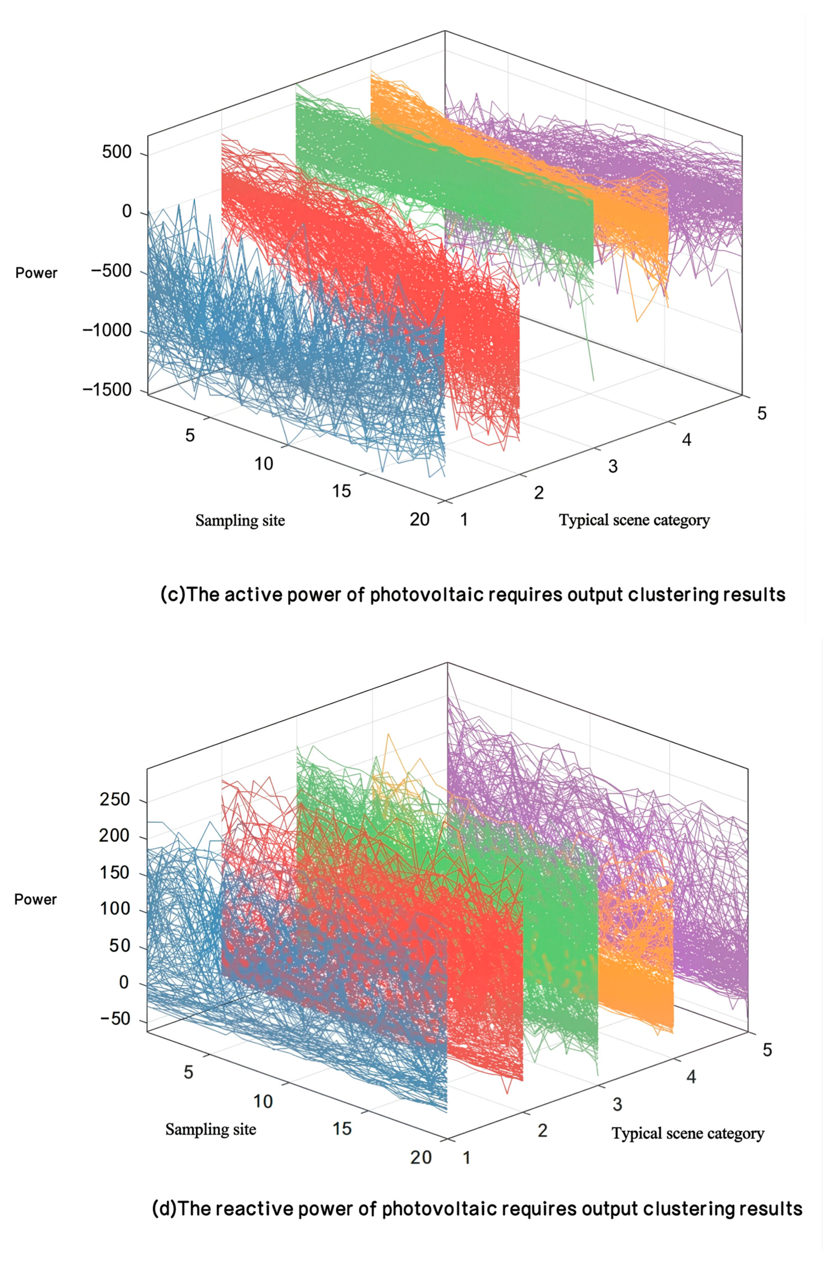
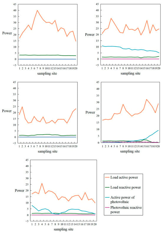
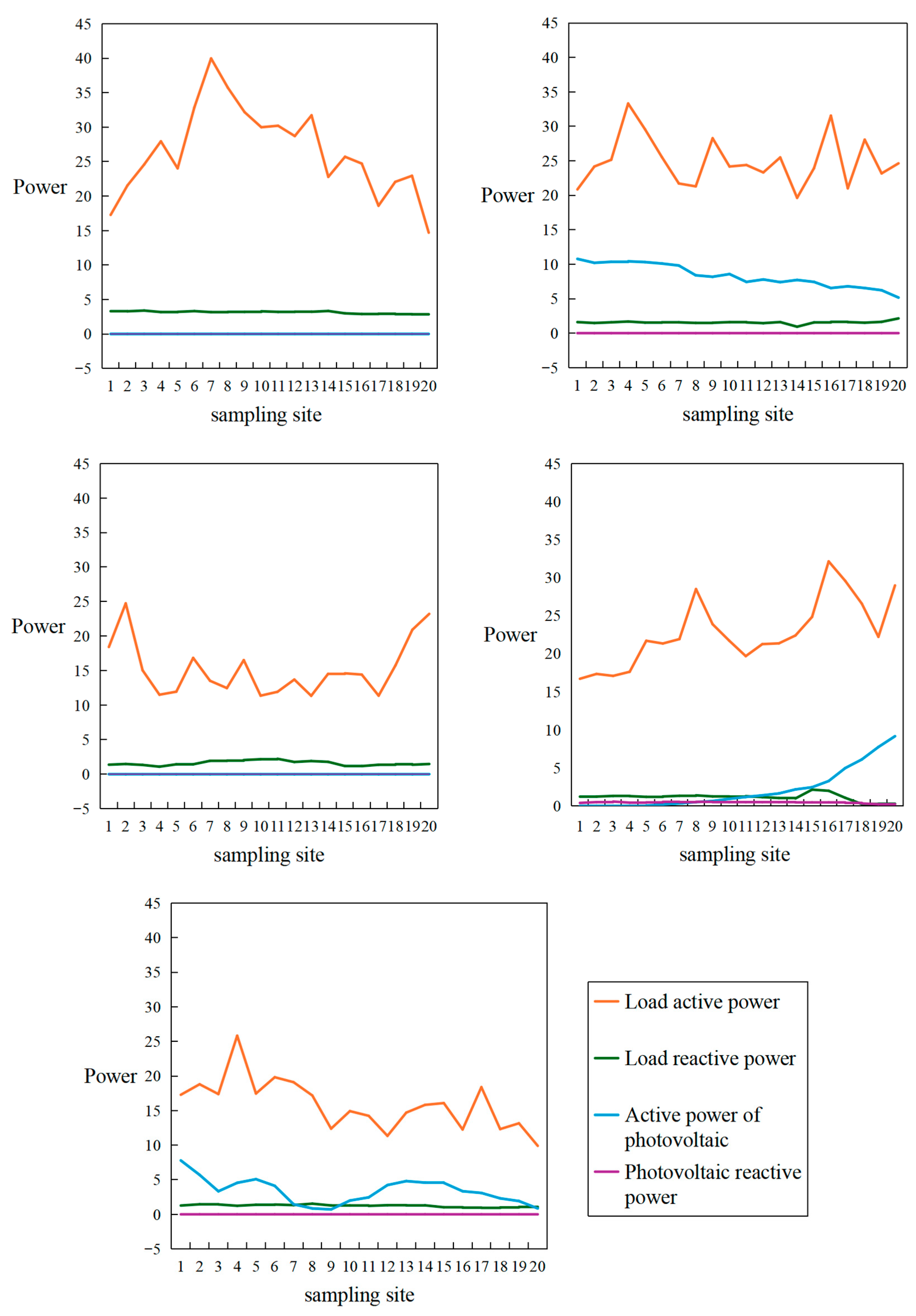
Considering the temporal correlation of source-load output based on historical data, a scenario clustering method combining DTW and Kmedoids algorithms is adopted to extract typical scenarios. The clustering results of typical active and reactive power output scenarios for sources and loads are shown in Figure 3.

Figure 3. Clustering Results of Source-Load Active/Reactive Power Typical Output Scenarios.

The cluster center data of the typical scenario clustering results for each category are used as the input data of the reliability assessment model considering the grid-connected and off-grid characteristics of PV systems. The relationships between the source-load cluster centers of each typical scenario are illustrated in Figure 4.

Figure 4. Relationship Between Source-Load Clustering Centers.

Analysis of the clustering results reveals that the five source-load output scenarios correspond to different actual operating conditions.

Scenario 1: This represents “winter heating or continuous cloudy days”. The sustained high load is primarily driven by the continuous operation of electric heating and indoor lighting during cold or low-visibility periods. The flat zero-power PV curves in Figure 3c combined with this persistent demand create the highest reliability risk, as no local generation is available to mitigate potential faults.

Scenario 2: This depicts “spring/autumn clear daytimes”. The load is moderate and stable, reflecting standard commercial and domestic activities under mild temperatures. The abundant and consistent PV output provides a strong “safety cushion,” allowing for high load restoration capability during midday faults.

Scenario 3: This corresponds to “late-night or pre-dawn” operations. The load remains at its minimum “base” level as most human activities cease. The low magnitude of both load and PV curves results in the lowest operational stress on the grid.

Scenario 4: This illustrates the “summer morning to noon” transition. The gradual upward trend in load is driven by the progressive activation of air conditioning (cooling load) as ambient temperatures rise. This is fortunately matched by a synchronized increase in PV output, demonstrating a “natural hedging” effect that balances the grid.

Scenario 5: This captures the “evening peak transition”. The purple curves in Figure 3a show intense fluctuations, which are primarily attributed to the randomized and intensive start-up of residential appliances (e.g., cooking, cleaning, and entertainment) and lighting as residents return home. This volatile demand coincides with the rapid extinction of PV output in Figure 3c, creating a critical “duck curve” impact. The sharp increase in net load during this window significantly stresses the tie-lines and necessitates precise MILP-based load transfer strategies.

Based on practical operational experience, Scenario 1 (high load in winter) and Scenario 4 (dynamic matching in summer) have a relatively high occurrence probability (approximately 25–30%), followed by Scenario 2 (PV output in spring and autumn) and Scenario 5 (evening transition) with a moderate probability (approximately 20% each), while Scenario 3 (low load in late night) has the lowest probability (approximately 10%). Therefore, in the case study verification of this chapter, the occurrence probabilities of Scenarios 1 to 5 are set to 25%, 20%, 10%, 25%, and 20%, respectively.

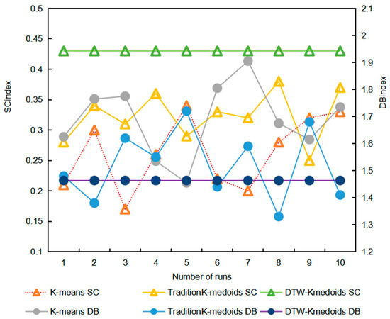
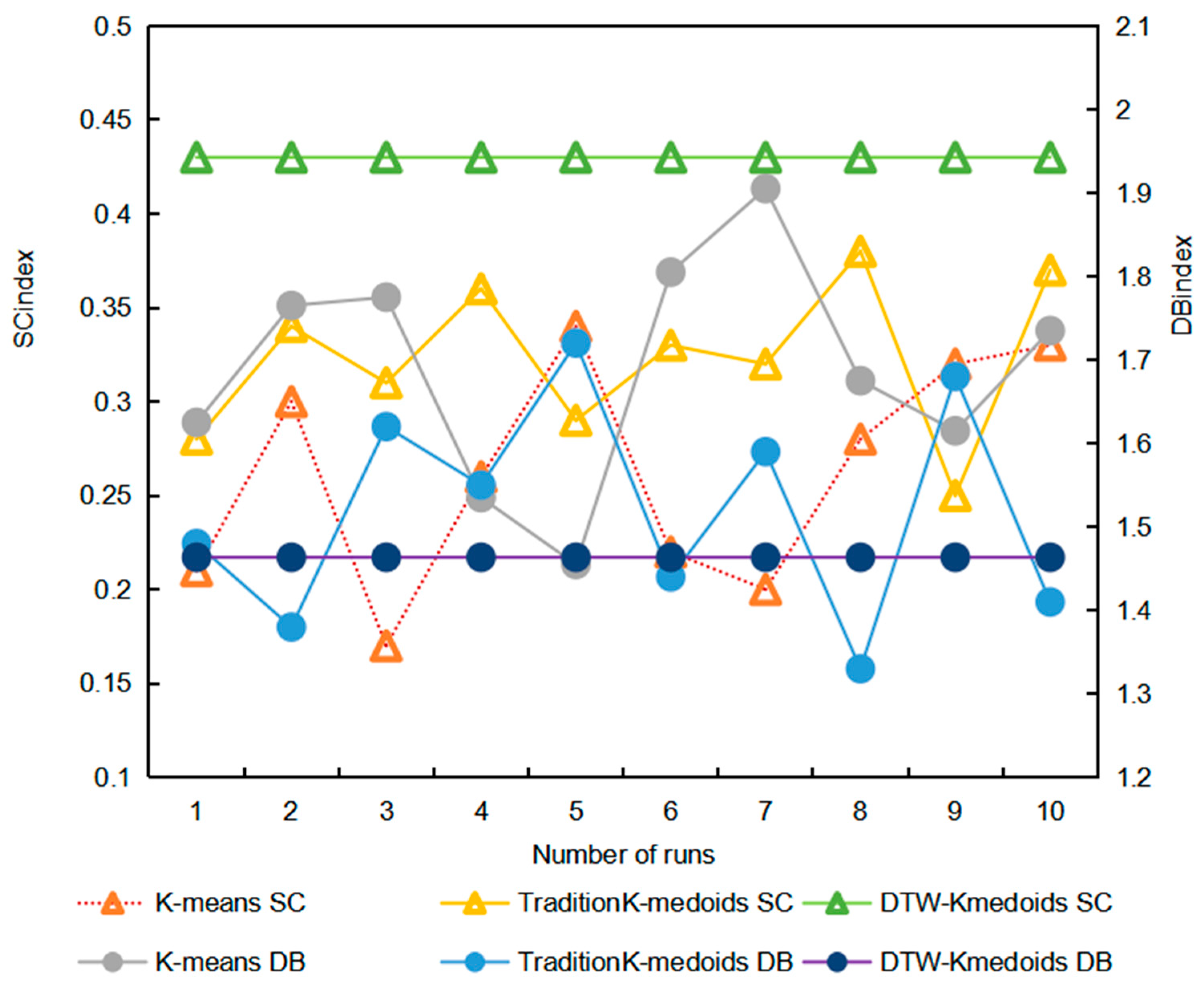
To rigorously demonstrate the success of the scenario clustering, the Silhouette Coefficient [32] (SC) and the Davies–Bouldin [33] (DB) index are introduced. The SC metric concurrently measures intra-cluster compactness and inter-cluster separation (a value closer to 1 indicates highly dense and well-separated clusters), while the DB index evaluates the ratio of intra-cluster scatter to inter-cluster separation (a lower value indicates superior clustering performance). As depicted in Figure 5, the three algorithms were executed 10 times with random initializations to test algorithmic stability. The traditional Euclidean-based K-means and Kmedoids exhibit severe fluctuations and inferior metric scores across different runs, struggling with the temporal shifts in the source-load curves. In contrast, the proposed DTW–Kmedoids algorithm consistently achieves the highest SC (stabilized at approximately 0.43) and the lowest DB index (stabilized at approximately 1.47) without fluctuation. This quantitative comparison strongly proves that incorporating DTW successfully aligns the temporal phase-shift features of PV and load curves. Consequently, the proposed method maximizes inter-cluster separation and intra-cluster compactness, ensuring the generated typical scenarios are highly representative and reliable for the subsequent reliability assessment.

Figure 5. Comparison of Clustering Metrics for Three Algorithms.

4.4. Analysis of Reliability Assessment Results Based on Typical Scenarios

The reliability assessment method for distribution networks considering the on-grid and off-grid characteristics of distributed power sources that was established was adopted to evaluate the reliability of typical scenarios obtained through clustering. The reliability index results of the distribution network are shown in Table 1.

Table 1. System Reliability Indices of Distribution Network under Typical Scenarios.

	SAIDI	SAIFI	EENS	ASAI
Typical Scenarios1	3.85	2.10	28.60	99.57
Typical Scenarios2	0.55	0.35	5.20	99.94
Typical Scenarios3	2.15	1.25	18.90	99.76
Typical Scenarios4	2.70	1.50	21.30	99.69
Typical Scenarios5	1.25	0.85	12.50	99.86
Overall Indicators	2.21	1.27	17.91	99.75

As shown in Table 1, significant differences in reliability levels are observed across typical scenarios due to distinct operating conditions. Scenario 1 (winter nights/cloudy days) exhibits the poorest reliability (SAIDI = 3.85 h/year) attributed to high load peaks, no PV output, and excessive stress on the main grid. Scenario 2 (daytime in spring/autumn) achieves the optimal reliability (SAIDI = 0.55 h/year, ASAI = 99.94%) with a PV active power peak of 31.36 MW, dynamic matching with stable loads, reactive power support from grid-connected PV, and post-fault reconfiguration. Scenario 3 (late night/early morning) features the lowest load (9.96 MW) but moderate reliability due to the absence of PV support. Scenario 4 (summer morning to noon) exhibits relatively poor reliability (SAIDI = 2.70 h/year). This occurs despite the presence of active PV generation. The primary cause is a critical temporal mismatch during the early phase of this scenario. During summer mornings, air-conditioning loads surge rapidly as temperatures rise. While PV output is active and growing synchronously, it remains relatively weak in the early morning hours. It has not yet reached its peak capacity. Consequently, an ‘early-stage power deficit’ emerges. The weak PV generation is insufficient to provide adequate grid-connected support to relieve stress on tie-lines during heavy cooling demand. This forces the system to rely heavily on tie-lines for load transfer. The resulting tie-line congestion limits the success rate of reconfiguration. This ultimately degrades the average reliability for this scenario. Scenario 5 (evening) sees decreasing PV output that still assists the main grid, with SAIDI optimized to 1.25 h/year and EENS to 12.50 MWh/year via reconfiguration.

To quantify the impact of multi-stage reconfiguration, a ‘No Reconfiguration’ baseline was established for Scenarios 1 (extreme stress) and 5 (dynamic volatility). Crucially, without reconfiguration, distributed PV units remain off-grid due to the lack of grid-forming capabilities, forcing affected nodes to endure the full 3-h repair. Consequently, the baseline SAIDI for both scenarios is fixed at 6.75 h/year, with EENS at 48.5 MWh/year (S1) and 34.0 MWh/year (S5).

The proposed strategy yields distinct improvements. In Scenario 5, SAIDI plummets by 81.5% (to 1.25 h/year) and EENS to 12.50 MWh/year. This is driven by a strong synergy: reconfiguration enables PV re-synchronization to supply local loads, while moderate demand leaves ample tie-line capacity. Conversely, in Scenario 1, the SAIDI reduction is highly constrained (to 3.85 h/year). Here, zero PV output and tie-line saturation under heavy winter loads severely restrict load transfer. These results verify that reconfiguration efficacy is fundamentally dictated by the dynamic matching of PV support and network capacity.

A critical synthesis of the results underscores that the traditional cross-sectional (static) assessment often fails to reflect the true operational stress of the grid during the restoration phase. Unlike static models that “freeze” the system state at the moment of failure, the methodology proposed in this study accounts for the continuous source-load evolution within a 5-h restoration window post-fault. This temporal factor is vital because the reliability of a modern distribution network is not a static probability, but a dynamic transition. For instance, in scenarios where a fault occurs in the afternoon, a static assessment might suggest a safe margin; However, as the 5-h restoration progresses, the simultaneous decline of PV output and the rise in evening residential load can rapidly erode this margin. This dynamic transition exposes “hidden risks” that static methods simply cannot capture. By bridging the gap between the failure instant and the completion of restoration, the proposed temporal framework provides a more realistic and rigorous benchmark for utility operators.

The quantitative results further reveal that the dynamic matching between PV generation and load demand fundamentally dictates the system’s reliability performance. Notably, Scenarios 1 and 4 exhibit severely degraded reliability indices (i.e., significantly higher SAIDI, SAIFI, and EENS). This is primarily driven by the critical temporal superposition of peak load demands and insufficient PV power within the restoration window. Conversely, Scenarios 2 and 5 demonstrate enhanced resilience, benefiting directly from robust localized PV support. Furthermore, the findings highlight that mitigating outage losses requires more than static network adjustments; it heavily relies on the temporal coordination between the grid-connected power injection from PV units (once re-energized) and system-wide reconfiguration. A sequential restoration strategy proves most effective. In this strategy, once PV units are reconnected to the grid through post-fault network reconfiguration, they provide local active and reactive power support, thereby alleviating stress on tie-lines and facilitating further load transfer. For high-volatility scenarios characterized by severe temporal mismatches, the strategic deployment of energy storage systems and fast-response control strategies will be a crucial pathway for future reliability enhancement.

4.5. Method Comparison and Generalizability Analysis

To further verify the accuracy and efficiency of the reliability assessment method considering the typical source-load operation scenarios proposed in this paper, the reliability assessment results of the proposed method were compared with those of three other methods: the reliability assessment without scenario clustering, the reliability assessment based on the Monte Carlo simulation method, and the reliability assessment based on the Traditional Static-profile Clustering (TSC) method. The reliability assessment results obtained by each method are shown in Table 2.

Table 2. Comparison of Reliability Assessment Results for Different Schemes.

	SAIDI (Hours/year)	SAIFI (Times/year)	EENS (MWh/year)	ASAI (%)	Solution Time (s)
	54	54	54	54	54
Monte Carlo simulation method	2.19	1.25	17.86	99.75	3672
Excluding scenario clustering	1.83	1.09	15.20	99.83	96
Traditional Static-profile Clustering	2.09	1.19	16.75	99.77	128
The proposed method	2.21	1.27	17.91	99.75	178

As shown in Table 2, the calculated results of the proposed method demonstrate high consistency with the Monte Carlo benchmark. The errors for both SAIDI and EENS are strictly maintained below 1%. This high precision stems from the temporal trajectory modeling. The DTW–Kmedoids clustering preserves the full dynamic evolution of sources and loads. During optimization, the multi-stage MILP model performs continuous temporal verification across the 5-h window. It captures voltage and capacity fluctuations at every time step. This rigorous verification logic aligns perfectly with Monte Carlo simulations.

In contrast, traditional techniques exhibit significant risk underestimation. The TSC yields an EENS error of 6.2%. The approach excluding clustering reaches a deviation of 14.9%. Calculated data indicate that TSC fails most severely in ‘Scenario 5 (Evening Transition)’. This method only extracts a single snapshot at the instant of failure. It assumes constant parameters throughout the restoration period. This ‘blindly optimistic’ logic ignores the PV decay risk at sunset. Once PV output vanishes, the system violates voltage and capacity constraints, leading to the collapse of the assumed restoration plan (or violation of operational constraints). TSC fails to identify these latent outage losses. These comparisons clearly prove that only the coupling of DTW–Kmedoids and multi-stage MILP can accurately capture the dynamic operational risks of active distribution networks.

4.6. Sensitivity Analysis of Photovoltaic Permeability and Switching Time

This section evaluates the method’s applicability across different PV capacities. We add four penetration scenarios (0%, 15%, 40%, and 60%) to the 25% baseline. Table 3 presents the weighted EENS results for the three methods.

Table 3. Comparison of EENS Using Three Methods under Different PV Penetration Rates.

PV Penetration Rate	Monte Carlo Simulation Method	Traditional Static-Profile Clustering	The Proposed Method
0	21.73	21.71 (−0.09%)	21.74 (+0.04%)
15	19.67	19.04 (−3.20%)	19.74 (+0.36%)
25	17.86	16.75 (−6.21%)	17.91 (+0.28%)
40	16.56	15.06 (−9.06%)	16.65 (+0.54%)
60	15.59	13.58 (−12.89%)	15.70 (+0.71%)

The results show high consistency between the proposed method and the Monte Carlo benchmark. The maximum relative error is only 0.71%. This proves that the DTW–Kmedoids and multi-stage MILP framework accurately replicates source-load dynamics. Furthermore, its accuracy remains insensitive to changes in PV capacity.

In contrast, TSC’s bias expands sharply as penetration increases. The underestimation bias grows from 6.21% at the baseline to 13.53% at 60% penetration. The error stems from TSC using a single static snapshot for the entire recovery window. It assumes constant PV output, which ignores key temporal features. This flaw is fatal in the evening transition (Scenario 5). TSC fails to perceive the sunset-induced drop in PV output. It extrapolates high initial output to the full window, overestimating tie-line transfer reserves. This leads to missed risks of load shedding from overloading. Additionally, TSC ignores the asynchronous growth of load and PV in Scenario 4.

In conclusion, static methods cannot meet accuracy requirements for high-PV networks. They ignore temporal coupling. By embedding continuous trajectories, the proposed method corrects the optimistic bias of static assessments. It provides a reliable quantitative baseline for network planning under various PV penetration levels.

As Table 4 shows, the benchmark EENS increases linearly as the switching time ${\tau }_{xy}^{SW}$ extends. The proposed method accurately quantifies the actual load loss risk under various switching delay conditions. The maximum evaluation error is only 0.69%. This indicates that the proposed model maintains extremely high accuracy regardless of the switching speed. It adapts perfectly to both 0.1 h rapid automated isolation and 2.0 h delayed manual operation. This fully proves the effectiveness and strong generalization capability of the proposed algorithm.

Table 4. System EENS under Different Switching Interruption Times.

$\mathbf{Switching} \mathbf{Time} {\mathit{\tau }}_{\mathit{x}\mathit{y}}^{\mathit{S}\mathit{W}}$	Monte Carlo Simulation Method	Traditional Static-Profile Clustering	The Proposed Method
0.1 h	14.53	13.58 (−6.54%)	14.58 (+0.34%)
0.5 h	17.86	16.75 (−6.21%)	17.91 (+0.28%)
1 h	22.02	19.38 (−11.99%)	22.14 (+0.54%)
2 h	30.35	23.58 (−22.31%)	30.56 (+0.69%)

In contrast, the error of the traditional TSC method surges non-linearly as ${\tau }_{xy}^{SW}$ extends. When ${\tau }_{xy}^{SW}$ reaches 2.0 h, the underestimation bias of TSC jumps to 22.31%. This error stems from the “information lag effect”. TSC formulates its reconfiguration scheme relying solely on the static snapshot at the fault instant. However, when the switches actually close after a long delay, the real source-load states (such as severe PV decay) have drastically changed. Forcibly executing an outdated static topology triggers severe tie-line overloads. This forces large amounts of load to be shed, causing a non-linear surge in actual outage losses.

In conclusion, the proposed method completely eliminates the decision-making blind spots of static assessments. It provides highly accurate quantitative evaluations under various dispatch response parameters. This further verifies its effectiveness and generalizability in active distribution networks with high PV penetration.

5. Conclusions

To overcome the “information lag” inherent in traditional reliability assessments, this paper developed a dynamic evaluation framework combining DTW–Kmedoids clustering with a multi-stage physical optimization model. Unlike conventional methods that rely on single static snapshots, our approach embeds continuous source-load trajectories into the entire fault restoration process. This successfully bridges the long-standing gap between stochastic time-series modeling and deterministic grid operations.

Evaluations demonstrate both the computational efficiency and the practical necessity of this dynamic approach. The proposed framework accelerates the computation time from over 1 h (using the Monte Carlo benchmark) to approximately 178 s, while maintaining a marginal error of less than 0.71%. More importantly, the results expose a critical flaw in existing static models: a non-linear surge in estimation bias. When PV penetration reaches 60% or manual switching delays extend to 2 h, traditional methods underestimate the EENS by up to 22.31%. By tracking the dynamic changes in source and load during power outages, such as the severe “duck curve” impact during evening transitions, our strategy successfully guided load transfers, achieving an 81.5% reduction in the SAIDI.

The engineering significance of this study lies in shifting the paradigm of distribution network planning. We quantitatively prove that mitigating outage risks in active grids relies more heavily on the temporal coordination of distributed resources than on merely upgrading static line capacities. By eliminating the decision-making “blind spots” caused by static assessments, this framework equips utility operators with a highly reliable tool to accurately quantify risks and prevent severe load shedding during critical transition windows.

Despite these contributions, the current model assumes constant component failure rates and relies on deterministic trajectory inputs. Future research will focus on robust optimization techniques to accommodate short-term forecasting errors, alongside the integration of energy storage systems, to further enhance system resilience against extreme weather disturbances.

References

- Ren, C.; Rong, F. Vulnerability assessment method of distribution network including distributed power and energy storage access. In Advances in Intelligent Systems, Computing and Sustainable Development; Rong, F., Ren, C., Eds.; Lecture Notes in Electrical Engineering; Springer: Singapore, 2025; Volume 1310, pp. 1–8. [Google Scholar] [CrossRef] [Scilit]
- Jooshaki, M.; Abbaspour, A.; Fotuhi-Firuzabad, M.; Muñoz-Delgado, G.; Contreras, J.; Lehtonen, M.; Arroyo, J.M. Linear formulations for topology-variable-based distribution system reliability assessment considering switching interruptions. IEEE Trans. Smart Grid 2020, 11, 4032–4043. [Google Scholar] [CrossRef] [Scilit]
- Zhang, Y.; Xu, J.; Beer, M. A Single-Loop Time-Variant Reliability Evaluation via a Decoupling Strategy and Probability Distribution Reconstruction. Reliab. Eng. Syst. Saf. 2023, 232, 109031. [Google Scholar] [CrossRef] [Scilit]
- Jooshaki, M.; Lehtonen, M.; Fotuhi-Firuzabad, M.; Muñoz-Delgado, G.; Contreras, J.; Arroyo, J.M. On the explicit formulation of reliability assessment of distribution systems with unknown network topology: Incorporation of DG, switching interruptions, and customer-interruption quantification. Appl. Energy 2022, 324, 119655. [Google Scholar] [CrossRef] [Scilit]
- Li, Z.; Wu, W.; Zhang, B.; Tai, X. Analytical reliability assessment method for complex distribution networks considering post-fault network reconfiguration. IEEE Trans. Power Syst. 2020, 35, 1457–1467. [Google Scholar] [CrossRef] [Scilit]
- Duan, D.-L.; Wu, X.-Y.; Deng, H.-Z. Reliability evaluation in substations considering operating conditions and failure modes. IEEE Trans. Power Deliv. 2012, 27, 309–316. [Google Scholar] [CrossRef] [Scilit]
- Arefi, A.; Ledwich, G.; Nourbakhsh, G.; Behi, B. A fast adequacy analysis for radial distribution networks considering reconfiguration and DGs. IEEE Trans. Smart Grid 2020, 11, 3896–3909. [Google Scholar] [CrossRef] [Scilit]
- Wang, C.; Zhang, T.; Luo, F.; Li, P.; Yao, L. Fault incidence matrix based reliability evaluation method for complex distribution system. IEEE Trans. Power Syst. 2018, 33, 6736–6745. [Google Scholar] [CrossRef] [Scilit]
- Conti, S.; Rizzo, S.A.; El-Saadany, E.F.; Essam, M.; Atwa, Y.M. Reliability assessment of distribution systems considering telecontrolled switches and microgrids. IEEE Trans. Power Syst. 2014, 29, 598–607. [Google Scholar] [CrossRef] [Scilit]
- Meera, P.S.; Hemamalini, S. Reliability Assessment and Enhancement of Distribution Networks Integrated with Renewable Distributed Generators: A Review. Sustain. Energy Technol. Assess. 2022, 54, 102812. [Google Scholar] [CrossRef] [Scilit]
- Chen, X.; Zhao, Y.; Xiong, W.; Yuan, X.; Zou, X. Partition and block algorithm for active distribution network reliability evaluation with a soft open point. In Proceedings of the 2023 5th Asia Energy and Electrical Engineering Symposium (AEEES), Chengdu, China, 24–26 March 2023; pp. 777–783. [Google Scholar] [CrossRef] [Scilit]
- Li, Y.; Li, G.; Sun, S.; Zhang, X.; Bie, Z. Reliability Assessment of Active Distribution Network Considering Path-Based Post-Fault Island Division. In Proceedings of the 6th International Conference on Energy, Electrical and Power Engineering (CEEPE), Guangzhou, China, 12–14 May 2023; pp. 618–623. [Google Scholar] [CrossRef] [Scilit]
- Luo, H.; Li, Y.; Li, X.; Gao, B.; Yan, Z.; Zhang, Q. Reliability Analysis and Research of Distribution Network Based on Sequential Monte Carlo Method. In Proceedings of the 2nd Asia-Pacific Conference on Communications Technology and Computer Science (ACCTCS), Shenyang, China, 25–27 February 2022; pp. 169–172. [Google Scholar] [CrossRef] [Scilit]
- Zhang, H.; Song, X.; Guo, S.; Yan, M. Reliability analysis of loess backfilling slope stability by Monte Carlo simulation. In Proceedings of the 2022 16th IEEE International Conference on Signal Processing (ICSP), Beijing, China, 21–23 October 2022; pp. 348–353. [Google Scholar] [CrossRef] [Scilit]
- Qin, Y.; Wang, J.; Ren, S.; Li, Z. Prediction of EV random charging load based on Monte Carlo simulation method. In Proceedings of the 2023 3rd International Conference on New Energy and Power Engineering (ICNEPE), Huzhou, China, 24–26 November 2023; pp. 295–298. [Google Scholar] [CrossRef] [Scilit]
- Su, S.; Hu, Y.; He, L.; Yamashita, K.; Wang, S. An assessment procedure of distribution network reliability considering photovoltaic power integration. IEEE Access 2019, 7, 60171–60185. [Google Scholar] [CrossRef] [Scilit]
- Bai, H.; Miao, S.; Zhang, P.; Bai, Z. Reliability evaluation of a distribution network with microgrid based on a combined power generation system. Energies 2015, 8, 1216–1241. [Google Scholar] [CrossRef] [Scilit]
- Liu, J.; Sun, K.; Ding, Z.; Li, K.-J.; Sun, Y. Multi-Stage Planning of Distribution Network with High Penetration Renewable Energy Considering Reliability Index. IEEE Trans. Ind. Appl. 2024, 60, 2344–2356. [Google Scholar] [CrossRef] [Scilit]
- Urgun, D.; Singh, C.; Vittal, V. Importance Sampling Using Multilabel Radial Basis Classification for Composite Power System Reliability Evaluation. IEEE Syst. J. 2020, 14, 2791–2800. [Google Scholar] [CrossRef] [Scilit]
- Borges, C.L.T. An Overview of Reliability Models and Methods for Distribution Systems with Renewable Energy Distributed Generation. Renew. Sustain. Energy Rev. 2012, 16, 4008–4015. [Google Scholar] [CrossRef] [Scilit]
- Liu, W.; Li, L.; Hu, J.; He, X.; Zhang, Y.; Wu, J. A long-term reliability assessment method for active distribution networks considering the impacts of extreme weather events. In Proceedings of the 2023 3rd International Conference on Energy Engineering and Power Systems (EEPS), Dali, China, 28–30 July 2023; pp. 1025–1030. [Google Scholar] [CrossRef] [Scilit]
- Nakamura, A.; Alsharif, F.; Umemura, A.; Takahashi, R.; Tamura, J.; Sakahara, A.; Tosaka, F.; Nakamoto, R. Voltage Control and Virtual Synchronous Generator Control of HVDC Interconnection Line for Improving Stability of Power System Including Large-Scale Wind Farm. IET Gener. Transm. Distrib. 2021, 15, 3375–3387. [Google Scholar] [CrossRef] [Scilit]
- Luo, F.; Bu, Q.; Ye, Z.; Yuan, Y.; Gao, L.; Lv, P. Dynamic Reconstruction Strategy of Distribution Network Based on Uncertainty Modeling and Impact Analysis of Wind and Photovoltaic Power. IEEE Access 2024, 12, 64069–64078. [Google Scholar] [CrossRef] [Scilit]
- Nebuloni, R.; Ilea, V.; Bovo, C.; Berizzi, A.; Arrigoni, C.; Re, F.; Bonera, R. Optimal Reconfiguration of Radial Distribution Networks with Renewable Energy Resources by Considering Configuration Shift Steps. Sustain. Energy Grids Netw. 2025, 43, 101861. [Google Scholar] [CrossRef] [Scilit]
- Miraftabzadeh, S.M.; Colombo, C.G.; Longo, M.; Foiadelli, F. K-Means and Alternative Clustering Methods in Modern Power Systems. IEEE Access 2023, 11, 119596–119633. [Google Scholar] [CrossRef] [Scilit]
- Kate, R.J. Using dynamic time warping distances as features for improved time series classification. Data Min. Knowl. Discov. 2016, 30, 283–312. [Google Scholar] [CrossRef] [Scilit]
- Tsuda, N.; Hamasuna, Y. Controlled-Sized Clustering for Time-Series Data. In Proceedings of the 2020 Joint 11th International Conference on Soft Computing and Intelligent Systems and 21st International Symposium on Advanced Intelligent Systems (SCIS-ISIS), Hachijo Island, Japan, 5–8 December 2020; pp. 1–5. [Google Scholar] [CrossRef] [Scilit]
- Shi, C.; Wei, B.; Wei, S.; Wang, W.; Liu, H.; Liu, J. A quantitative discriminant method of elbow point for the optimal number of clusters in clustering algorithm. EURASIP J. Wirel. Commun. Netw. 2021, 2021, 31. [Google Scholar] [CrossRef] [Scilit]
- Brown, R.E. Electric Power Distribution Reliability, 2nd ed.; CRC Press: Boca Raton, FL, USA, 2017. [Google Scholar] [CrossRef] [Scilit]
- Su, Y.; Liu, F.; Kang, K.; Wang, Z. Implicit Sparsity of LinDistFlow Model. IEEE Trans. Power Syst. 2023, 38, 4966–4969. [Google Scholar] [CrossRef] [Scilit]
- Huang, G.; Zhou, Y.; Yang, C.; Zhu, Q.; Zhou, L.; Dong, X.; Li, J.; Zhu, J. Optimal allocation method of circuit breakers and switches in distribution networks considering load level variation. Processes 2023, 11, 2235. [Google Scholar] [CrossRef] [Scilit]
- Gao, M.; Gong, T.; Lin, R.; Zou, H. A Power Load Clustering Method Based on Limited DTW Algorithm. In Proceedings of the 2019 IEEE 3rd Information Technology, Networking, Electronic and Automation Control Conference (ITNEC), Chengdu, China, 15–17 March 2019; pp. 253–256. [Google Scholar] [CrossRef] [Scilit]
- Jin, J.; Ye, L.; Li, J.; Zhao, Y.; Lu, P.; Wang, W. Wind and Photovoltaic Power Time Series Data Aggregation Method Based on an Ensemble Clustering and Markov Chain. CSEE J. Power Energy Syst. 2022, 8, 757–768. [Google Scholar] [CrossRef] [Scilit]
Disclaimer/Publisher’s Note: The statements, opinions and data contained in all publications are solely those of the individual author(s) and contributor(s) and not of MDPI and/or the editor(s). MDPI and/or the editor(s) disclaim responsibility for any injury to people or property resulting from any ideas, methods, instructions or products referred to in the content. |
© 2026 by the authors. Licensee MDPI, Basel, Switzerland. This article is an open access article distributed under the terms and conditions of the Creative Commons Attribution (CC BY) license.