


Abstract
Industrial equipment data often exhibit high dimensionality and class imbalance, which make it difficult to achieve both accurate failure detection and identification of the factors contributing to failures. To address this issue, this study proposes an explainable failure classification framework, Feature-Wise Attention Graph Convolutional Network (FWA-GCN), which combines Feature-Wise Attention (FWA) with a Graph Convolutional Network (GCN) to provide both high classification performance and variable-level interpretability. In the proposed model, tabular sensor records are treated as nodes, and a similarity-based graph is constructed to capture relationships among samples. Feature-Wise Attention learns the importance of each feature and reweights node features accordingly, and the reweighted features are then used as input to the GCN to classify failure occurrences. To alleviate the class imbalance problem, a weighted loss function is applied during training by assigning a higher weight to the failure class. Experiments conducted on the Air Pressure System (APS) dataset demonstrate that the proposed FWA-GCN achieves Precision of 79.95%, Recall of 85.07%, and F1-score of 82.43%, outperforming conventional machine learning models including Random Forest, XGBoost, CatBoost, and Multi-Layer Perceptron, as well as a standard GCN model. Furthermore, an ablation study was conducted by removing the top features selected by the attention mechanism. The results show a significant decrease in recall, confirming the effectiveness of the attention-based feature importance and supporting the interpretability of the proposed framework.
1. Introduction
As industrial automation control systems and sensor-driven operations become more widespread, the volume of data generated across multiple process stages is rapidly increasing, and the complexity and interdependence of equipment systems are also growing [1]. Recently, this trend has expanded toward smart manufacturing systems that adopt digital twins to synchronize the states of individual equipment and processes in a virtual space. Through this integration, data and state information from multiple pieces of equipment can be linked to manage the overall process in a unified manner, evolving into a Digital Twin Network–type architecture [2]. As data accumulate at scale and operational structures become more complex, the need for data-driven diagnostic technologies grows in order to detect subtle changes that signal abnormal process behavior at an early stage and to prevent operational downtime.
Because real industrial processes in automotive and manufacturing plants are complex and dynamically changing, alarms based solely on predefined fixed thresholds or expert rules have limitations in effectively identifying anomalous signs [3]. If such anomalies are not detected in time, equipment failures and production interruptions may occur, leading to reduced productivity and increased maintenance costs. Therefore, as sensor-based condition monitoring data accumulate in manufacturing sites, machine learning- and deep learning-based anomaly detection—learning patterns of normal behavior from data and detecting deviations at an early stage—has become a key enabling technology [4,5,6,7,8,9]. However, in practical deployment, most manufacturers’ datasets exhibit severe class imbalance, where normal samples overwhelmingly outnumber failure cases [10,11]. In such settings, improving precision alone is insufficient. From a maintenance cost perspective, the cost of handling incidents caused by missed failures is often much higher than the cost of routine inspections; thus, failure diagnosis models must achieve high recall to reduce missed detections while maintaining precision.
As one approach to mitigating class imbalance, smart manufacturing systems have explored the use of digital twins to reproduce rare failure scenarios in virtual environments and augment data, thereby alleviating data imbalance [12,13]. However, data collected in virtual environments may not adequately capture unpredictable environmental noise, subtle vibrations, or complex interactions among fine-grained variables, which can lead to distribution gaps from real operational data. In addition, prior industrial failure diagnosis studies have applied sampling techniques such as the Synthetic Minority Over-Sampling Technique (SMOTE) [14,15,16,17] or focused on improving classification performance using traditional machine learning algorithms [18,19,20], including Random Forest [21], Support Vector Machine (SVM) [22], and XGBoost [23]. These methods can be effective in reducing overall errors, but they are limited in fully leveraging inter-feature relationships or structural information [24,25]. Industrial failures often appear not as anomalies in a single sensor, but as concurrent changes and interaction patterns across multiple sensor variables; thus, without modeling inter-feature relationships, both false positives and false negatives may increase.
Moreover, even when deep learning models improve predictive performance, they often suffer from a black-box issue, making it difficult to explain which sensor signals drive a failure decision. Practitioners in the field require clear, feature-level diagnostic evidence that supports immediate corrective actions, beyond a simple failure alarm.
To address these challenges, this study proposes a supervised failure detection framework, Feature-Wise Attention Graph Convolutional Network (FWA-GCN), which simultaneously considers class imbalance and interpretability. Existing GNN studies on tabular data have mainly focused on modeling relationships among samples and improving anomaly detection performance. However, studies that jointly address failure detection under class-imbalanced conditions and feature-level interpretability remain limited. The objectives of this study are as follows.
- To select sensors that contribute to discriminative performance in binary failure detection, we compute feature importance using the Gini importance from a Random Forest. Since multivariate sensor data may include irrelevant or redundant variables, we select only the top-ranked features to reduce the input dimensionality and then apply normalization to minimize the influence of outliers.
- Conventional machine learning models process each sample independently, which limits their ability to model inter-sample relationships in tabular data. In this study, we compute inner-product similarity between samples in the selected feature space and construct a graph by creating edges that connect only the Top-k most similar neighbors.
- By dynamically emphasizing important features for each sample via Feature-Wise Attention, we suppress the influence of noisy features and provide feature-level interpretability. In addition, by combining a class-ratio–based weighted loss function with threshold optimization, we effectively reduce missed failure detections even under severe class imbalance.
The paper is organized as follows. Section 1 introduces the research background and problem statement. Section 2 reviews related work on failure detection in industrial systems and graph-based learning. Section 3 describes the proposed Feature-Wise Attention Graph Convolutional Network (FWA-GCN) framework, including the graph construction algorithm and the mathematical formulation of the attention mechanism. Section 4 presents experiments and results on the APS Failure dataset, including comparisons with Random Forest (RF), XGBoost, CatBoost, Multi-Layer Perceptron (MLP), and GCN. We also conduct an ablation study by masking attention-selected features to verify whether the selected features truly affect detections, thereby assessing the reliability of the interpretability. Finally, Section 5 summarizes the main contributions and discusses future research directions.
2. Related Work
In this section, we review prior studies on anomaly detection for industrial systems and analyze the contributions and limitations of each approach. Specifically, Section 2.1 examines conventional machine learning and deep learning-based anomaly detection methods, while Section 2.2 discusses graph construction methodologies for learning latent structure from tabular data, thereby clarifying the technical distinctiveness of the framework proposed in this study.
2.1. Anomaly Detection Methods for Industrial Systems
Recent research on industrial anomaly detection has expanded toward lightweight machine learning models for practical deployment, unsupervised learning to address limited labels, and ensemble models designed for real-time operation. For example, Aly proposed an optimized Logistic Boosting model for factory IoT environments, demonstrating improved performance compared with RF and SVM. This method repeatedly assigns higher weights to misclassified instances, enabling effective learning of rare anomalies through boosting [26]. In many industrial settings, however, failure labels are scarce. To address this, Panza et al. proposed an unsupervised approach trained only on normal data, where anomalies are detected by computing an anomaly score based on the deviation between the model’s predictions and the observed values [27]. From the perspective of real-time deployment, David et al. combined Local Outlier Factor (LOF), One-Class Support Vector Machine (OCSVM), and an Autoencoder using a weighted averaging scheme, and proposed a hybrid ensemble pipeline that separates the manufacturing phase from the operational phase, achieving better performance than individual models [28]. Carletti et al. applied a deep learning–based anomaly detection method to sensor time-series data from a refrigerator manufacturing process and assigned anomaly scores to each pressure profile, reporting improved performance over traditional handcrafted-feature approaches [29]. However, many of the above studies process tabular data at the individual-sample level, making it difficult to structurally incorporate relationships among data samples. To address this limitation, we construct a similarity-based graph between samples and leverage information from neighboring samples jointly.
2.2. Graph Structure Learning for Tabular Data
Most data generated in modern industries are represented in tabular form. Sensor data from manufacturing processes and network traffic logs are typical examples of structured data composed of rows and columns. Anomaly detection on such tabular data has traditionally been studied using statistical approaches such as Isolation Forest and One-Class SVM (Support Vector Machine) [30,31,32,33], as well as deep learning models including Autoencoders and Multi-Layer Perceptron (MLP) [34,35,36]. However, these approaches treat each data sample independently, which limits their ability to capture interactions among samples or complex dependencies among variables, thereby restricting detection performance.
To overcome these limitations, recent studies have explored representing relationships among data samples or variables as graph structures and incorporating them into the learning process [37,38,39,40,41,42]. For example, LUNAR (Learnable Unified Neighborhood-based Anomaly Ranking) defines each data sample as a node and constructs a graph by connecting each node to its k nearest neighbors. Instead of using the original node attributes, the model uses edge features defined by the distances between nodes and their neighbors, and a Graph Neural Network (GNN) aggregates these distance vectors through a learnable function to compute anomaly scores [43]. While this approach can be viewed as a learnable extension of traditional distance-based anomaly detection methods such as k-NN and Local Outlier Factor (LOF), its focus on distance information rather than individual feature values limits feature-level interpretability.
Similarly, Prototype-oriented Hypergraph Representation Learning for Anomaly Detection (PHAD) introduces hypergraphs instead of simple graphs to model complex relationships among samples in tabular data [44]. In this approach, a single hyperedge can connect multiple nodes simultaneously, enabling the representation of higher-order correlations among data instances. However, when applied to high-dimensional data, the resulting structure may become complex and computationally expensive. Meanwhile, Graph Regularized Autoencoder constructs a graph based on pairwise distances between all data samples and retains only the essential connections using a Minimum Spanning Tree (MST) to learn latent relationships [45]. These studies are meaningful in that they attempt to incorporate latent relationships within tabular data through graph-based representations.
The approach of learning tabular data through graph representations has recently evolved in two main directions. One approach defines each data instance as a node and constructs a graph based on similarity or adjacency relationships among samples [38,43,44,45]. The other approach defines each feature as a node and explicitly models interactions among variables [46,47]. The former is effective for capturing relationships among samples, but it may be difficult to directly explain which input variables contribute most to the prediction. In contrast, the latter has strengths in modeling dependencies among variables, but its structure can become complex when applied to sample-wise failure classification tasks involving high-dimensional industrial tabular data. Moreover, many graph-based anomaly detection studies assume that the graph structure is originally given or focus on unsupervised anomaly detection settings [37,41,42], which differ from industrial tabular failure classification problems such as the APS dataset.
In contrast, this study uses a similarity graph in which each sample in the APS dataset is treated as a node, while incorporating feature-wise attention-based reweighting before graph convolution to selectively emphasize input variables that are important for failure classification. Rather than proposing a completely new GNN operation, this study focuses on designing and validating a graph-based classification framework tailored to high-dimensional and imbalanced APS tabular data. In particular, by combining a sample similarity graph with feature-wise reweighting, this study analyzes both the applicability and limitations of graph-based learning for industrial failure classification problems.
3. Methods
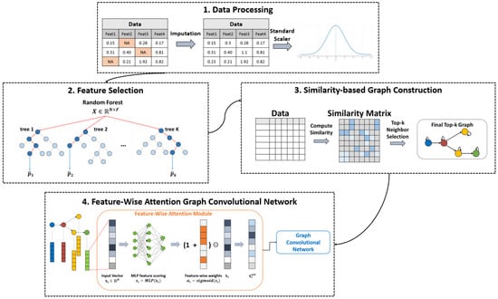
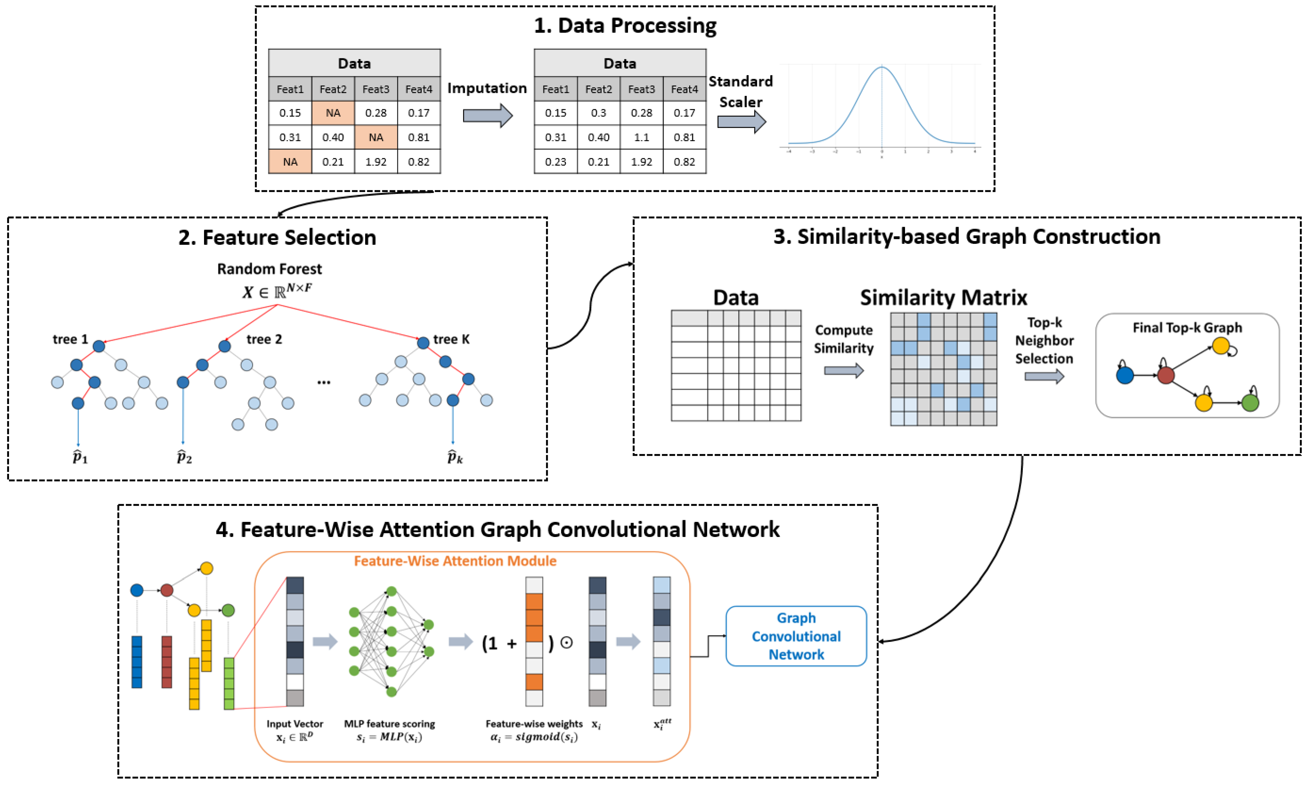
In this study, we propose the FWA-GCN framework to accurately classify failures in industrial sensor data that are high-dimensional and highly imbalanced. The overall framework consists of the following components, as illustrated in Figure 1.
Figure 1.
Feature-Wise Attention Graph Convolutional Network Workflow.
- Feature Selection: We reduce the input dimensionality by selecting features that are most informative for distinguishing failure from normal in a binary failure detection task.
- Similarity-based Graph Construction: We construct a graph by computing inter-sample similarity in the selected feature space, and control the message-passing computation and memory usage during GCN training via Top-k sparsification.
- FWA-GCN: We learn feature-level importance for each sample to reweight the input, and classify failures using the attention-weighted node features together with the constructed graph structure.
3.1. Problem Statement
We consider a binary classification task that detects whether a failure occurs from APS sensor-based data. The dataset consists of N samples, where each sample i is represented by an F-dimensional numerical feature vector. Here, yi = 1 denotes a failure and yi = 0 denotes a normal condition:
Given a training dataset , the goal of this study is to learn a classifier that can reliably distinguish the failure class even under severe class imbalance.
3.2. Feature Selection Based on Random Forest
Industrial data often contain many features and substantial noise, so using all variables as-is can increase computational cost and raise the risk of overfitting. Therefore, this study selects features that contribute most to distinguishing normal from faulty conditions using Random Forest (RF) importance based on impurity decrease. RF performs splits that reduce node impurity, and the accumulated impurity reduction before and after each split can be used to quantify each feature’s contribution to classification. Let p(c∣n) denote the proportion of class c ∈ {0, 1} at node n. For binary classification, the Gini impurity (G(n)) [48] is defined as:
where Nn is the total number of samples that reach node n in the tree, and Nn,c is the number of samples of class c among them. When node n is split by feature f into left and right child nodes nL and nR, the impurity decrease from this split is computed as a weighted reduction based on the sample proportions:
For a single decision tree T, the importance of feature f, denoted ImpT(f), is obtained by summing Δi(n,f) over all internal nodes n where f is used for splitting. Because higher-level nodes typically cover more samples, we weigh each term by the fraction of samples at node n relative to the root:
where NT is the set of internal nodes in tree T, v(n) is the feature used at node n, and Nroot is the total number of samples used to train the tree. Since RF is an ensemble of multiple trees, the forest-level feature importance is computed by averaging the tree-wise importances. Let M be the number of trees in the forest and Tt the t-th tree:
In this study, we apply a higher-class weight to the minority class when training the Random Forest (RF) to account for class imbalance. We then ranked features in descending order using the Gini importance of the RF trained on the training set, and jointly selected the number of top features D and the classification threshold τ that maximize the F1-score on the validation set. The selected D and τ were applied unchanged for evaluation on the test set.
3.3. Similarity-Based Graph Construction
Tabular data, such as sensor measurements, do not have an explicit graph structure. Therefore, to apply graph neural networks, it is necessary to define relationships between samples and construct a graph. In this study, we compute inter-sample similarity to define edges and generate a graph, under the assumption that samples exhibiting similar operating conditions or failure patterns are located close to each other in the feature space. Each sample is defined as a node, and the node feature matrix is given as follows,
where D is the number of selected features and each node i has a label yi ∈ {0, 1}. To reduce the influence of feature-vector magnitude and to compare pattern similarity, we apply L2 normalization:
We then compute a similarity matrix by taking inner products between the selected feature vectors. This can be interpreted as cosine similarity, where larger values indicate that the two samples have more similar feature patterns. In addition, to prevent negative similarity values from exerting excessive influence, we apply LeakyReLU and normalize the results with a row-wise softmax to obtain a connection-weight matrix P. Here Pij is used as the weight when node i receives a message from its neighbor j.
However, a fully connected graph substantially increases computational and memory costs during GCN training. Therefore, we limit the number of edges by connecting each node i only to its Top-k most similar neighbors j. We also add self-loops for training stability, so that each node has a total of k + 1 connections. The value of k is determined by comparing validation F1-scores over a candidate set, and we select the smallest value, k = 4, within the range where performance is similar, considering computational cost.
The similarity-based graphs were constructed independently for each split to prevent data leakage. Specifically, we computed separate similarity matrices and built separate graphs using only the samples within each of the Train, Validation, and Test splits. When constructing the Test graph, no feature information or label information from the Train or Validation data was used. This prevents transductive information mixing that can occur when the entire dataset is represented as a single graph, and maintains an inductive setting in which evaluation on unseen samples does not access information from other splits.
3.4. Feature-Wise Attention Graph Convolutional Network
This section describes the architecture and training procedure of the FWA-GCN, which classifies node-level failures using the D selected features from Section 3.2 and the similarity-based graph G = (V,E) constructed in Section 3.3. The proposed model consists of (i) a Feature-Wise Attention module that learns the importance of intra-node features and (ii) a GCN-based classifier that aggregates neighborhood information through the graph structure.
3.4.1. Feature-Wise Attention for Input Feature Re-Weighting
In tabular sensor data, the features explaining a failure may vary across samples, and a single failure can be reflected in multiple features simultaneously. Therefore, treating all features equally may allow non-informative features to negatively affect prediction performance. To mitigate this issue, this study learns feature-wise gate values for each node i with input vector , and reweights the input features accordingly. Specifically, for each feature k, the feature index embedding ek is combined with the actual feature value xi,k of node i, and an MLP is used to compute a feature score si,k:
Then, a sigmoid function is applied to obtain the feature-wise gate value
Here, αi,k ∈ (0, 1) represents an independent scaling factor indicating how strongly feature k should be emphasized for node i. The attention-refined input representation is computed as follows:
where ⨀ denotes element-wise multiplication. This formulation preserves the original input in a residual manner rather than replacing it entirely, while amplifying the magnitude of important features. Consequently, αi,k can be interpreted as the relative importance of feature k for failure classification at node i, and represents an input embedding that highlights features relevant to failure detection while retaining the original information.
3.4.2. Graph Convolutional Network for Failure Classification
Using the node features with Feature-Wise Attention applied and the graph G = (V, E, w), the GCN updates each node representation while aggregating information from neighboring nodes. Let H(l) denote the node representations at the l-th layer. A standard GCN update can be written as follows, where W(l) denotes trainable parameters and ϕ is a nonlinear activation function. is the normalized adjacency matrix with self-loops, defined by and .
In this study, we apply a linear classifier after two graph convolution layers and finally output the logit zi for node i. Here, pi denotes the probability that node i belongs to the failure class.
3.4.3. Loss Function and Imbalance-Aware Learning
Since the APS dataset is dominated by normal samples, the failure class may not be sufficiently reflected during training. To mitigate class imbalance, this study applies BCEWithLogitsLoss. For the logit zi of each node, the loss is defined as follows. Here, ω+ is the weight for the failure class and is set to reflect the class ratio in the training data.
In this study, letting the numbers of normal and failure samples in the training data be Nneg and Npos, respectively, we compute the failure-class weight as follows and apply it. This choice aims to increase the loss contribution of failure samples while alleviating training instability caused by overly large weights. The base weight is computed as the ratio between the numbers of normal and failure samples, which is approximately 59 for the APS training data. However, using this value directly can excessively amplify the contribution of failure samples in the loss function and lead to unstable training. To mitigate this, we apply a square root to the ratio and set the final weight to approximately 7.68. This is a data-driven choice that sufficiently increases the gradient contribution of failure samples while maintaining balance with normal samples. It is a principled approach computed directly from the class ratio without requiring an additional hyperparameter search.
4. Datasets and Proposed Framework
In this section, we conduct experiments to answer the following research questions.
- RQ1 (Failure Detection Performance): Does the proposed method improve APS failure detection performance compared with baseline models?
- RQ2 (Effect of Feature Selection on Classification Performance): Does Random Forest–based feature selection affect model performance?
- RQ3 (Effect of Graph Construction): How does a cosine-similarity–based graph influence the performance of FWA-GCN?
- RQ4 (Interpretability via Feature-Wise Attention): Does Feature-Wise Attention actually identify important features?
4.1. Datasets and Experimental Setup
To evaluate the proposed framework, we use the APS Failure dataset. The APS Failure dataset, collected from the UCI Machine Learning Repository, contains data from a fleet for large Scania trucks in daily operation. It focuses on the air pressure system, which supplies pressure to various components such as braking, gear shifting, stop signal switches, and air dryers [49].
The APS Failure dataset consists of 60,000 training samples and 16,000 test samples, with 170 sensor features. We further split the data as follows:
- Train: 48,000 × 170
- Validation: 12,000 × 170
- Test: 16,000 × 170
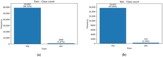
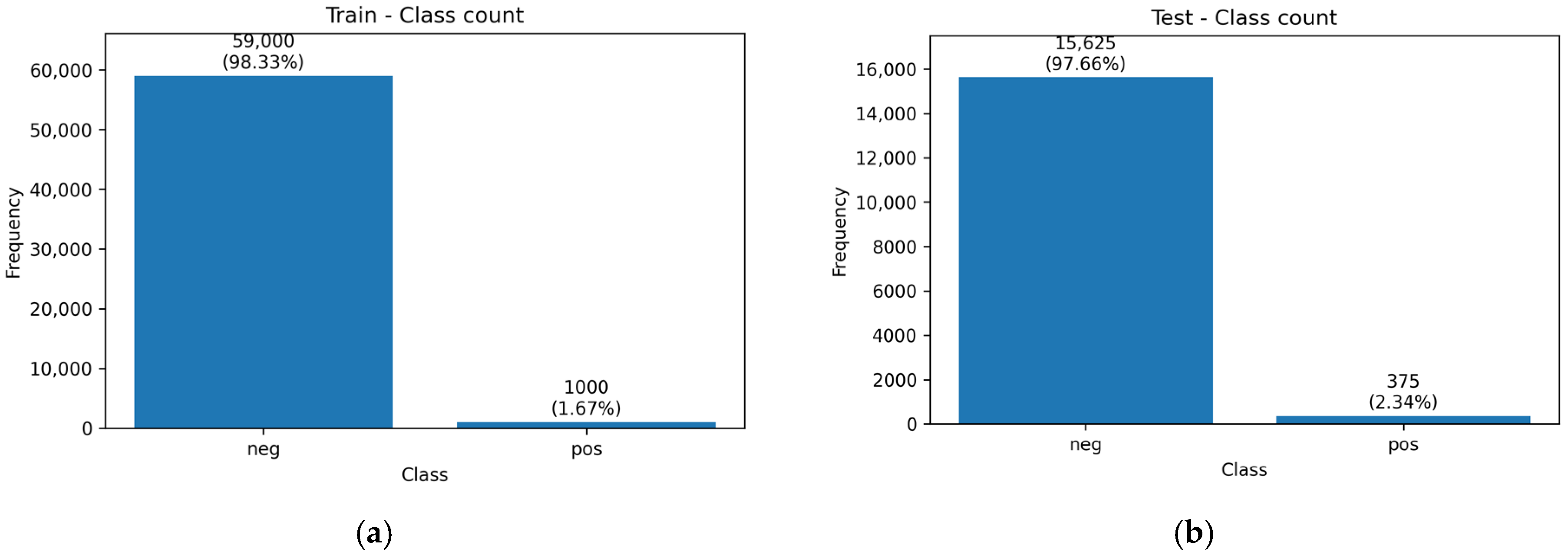
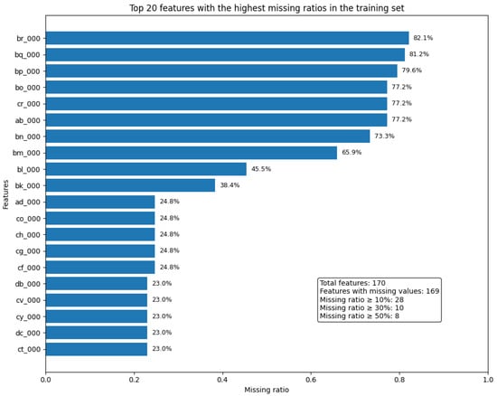
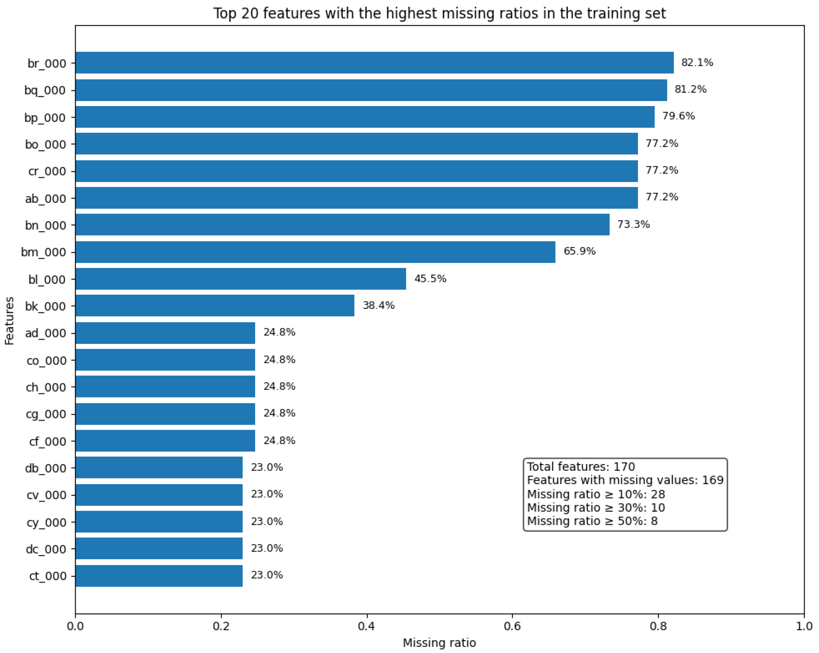
Samples are labeled as 0 for normal and 1 for failure. The training set exhibits severe class imbalance: among 60,000 training samples, 59,000 belong to the normal class, whereas only 1000 belong to the failure class. Figure 2 illustrates the class distribution of the training and test datasets, showing that both sets are highly imbalanced, with the negative class dominating the positive class. In addition, the dataset contains a substantial number of missing values. Figure 3 shows the missing-value ratio of the training features sorted in descending order. Several variables exhibit substantial missingness, and multiple features have missing ratios exceeding 30% and 50%, respectively. This indicates that the APS training set contains severe and non-uniform missing-value patterns, making appropriate imputation essential before model training.
Figure 2.
Class imbalance ratios of the training and test datasets: (a) class imbalance ratio in the training dataset; (b) class imbalance ratio in the test dataset.
Figure 3.
Missing values in the dataset.
Therefore, to prevent information leakage, missing values in the train, validation, and test sets were imputed using the median values computed from the training data. To mitigate class imbalance, we applied BCEWithLogitsLoss with a positive-class weight to MLP, GCN, and FWA-GCN, and used class weights for Random Forest so that the minority class is more strongly reflected during training. The major hyperparameters and class-imbalance handling methods of the tree-based models used for comparison (RF, XGBoost, and CatBoost) are presented in Table 1, while the network architectures and optimization settings of the deep learning models (MLP, GCN, and FWA-GCN) are provided in Table 2. All models were implemented using PyTorch version 2.3.0. Although the experimental environment included CUDA 12.1 and cuDNN 8.9.2, all training and inference were conducted in a CPU environment so that the models can be deployed in typical manufacturing settings where high-performance computing resources such as A100 or H100 GPUs are not available.
Table 1.
Hyperparameter settings of the compared machine learning models.
Table 2.
Hyperparameter settings of the compared deep learning models.
In all experiments, the best model was selected based on the validation loss, and for the comparison models, the final decision threshold (\tau) was set to maximize the F1-score on the validation set.
4.2. Baselines
To evaluate the failure classification performance of the proposed method, five representative machine learning and deep learning models widely used for tabular data classification were selected as baseline models.
- Random Forest (RF) [50]: An ensemble learning algorithm that constructs multiple decision trees and shows strong performance and robustness on tabular data. It can effectively learn nonlinear relationships.
- Extreme Gradient Boosting (XGBoost) [51]: XGBoost is a supervised learning algorithm based on Gradient Boosting Decision Trees (GBDT). It trains by sequentially adding decision trees to reduce the prediction errors of previous stages.
- Categorical Boosting (CatBoost) [52]: CatBoost is a supervised learning algorithm based on gradient boosting, designed to handle categorical features effectively. It reduces prediction bias through an ordered target-statistics scheme and provides stable training and strong predictive performance using symmetric tree structures.
- Multi-Layer Perceptron (MLP) [53]: A feed-forward artificial neural network composed of multiple layers of interconnected perceptron. It is used for various tasks such as complex pattern recognition, classification, and regression.
- Graph Convolutional Network (GCN) [54]: A deep learning model designed to analyze graph-structured data, extending the concept of CNNs to graphs. It aggregates and learns information from neighboring nodes to extract node-level or graph-level representations. It performs well when connectivity between nodes is important and generates node embeddings for tasks such as classification and prediction.
4.3. Evaluation Metrics
We use Precision, Recall, and F1-score to evaluate the performance of the proposed method and the baseline models by comparing their predictions with the ground-truth labels on the test dataset. In Equations (18)–(20), True Positive (TP) refers to cases where the model correctly predicts a positive sample as positive. False Positive (FP) refers to cases where the model incorrectly predicts a negative sample as positive, and False Negative (FN) refers to cases where the model incorrectly predicts a positive sample as negative. In class-imbalanced settings, F1-score alone is insufficient to fully evaluate overall model performance. Therefore, to provide a more reliable assessment under imbalance, we additionally report Precision–Recall Area Under the Curve (PR-AUC), Balanced Accuracy, and Matthews Correlation Coefficient (MCC). PR-AUC summarizes the precision–recall trade-off across different decision thresholds, while Balanced Accuracy corrects for imbalance by averaging the recall of the normal and failure classes. MCC is a balanced single metric that accounts for TP, TN, FP, and FN, and is particularly useful in class-imbalanced scenarios.
For accurate classification, we vary the threshold τ from 0 to 1 with a fixed step size and compute the F1-score on the validation dataset for each τ. We then select the value of τ that maximized the F1-score as the final threshold and applied it to the test dataset.
4.4. RQ1. Failure Detection Performance
This section compares the failure classification performance of Random Forest, XGBoost, CatBoost, MLP, GCN, and Feature-Wise Attention GCN on the APS dataset. The original APS data consist of 170 high-dimensional features, and using all variables may degrade performance or increase memory consumption due to unnecessary noise and redundant information. To address this issue, this study first trained a Random Forest model on the training set and ranked features based on Gini importance. The number of selected features, N, was then varied from 50 to 100 in increments of 5, and the optimal value was determined based on validation performance. As a result, the best validation performance was achieved when N = 75, which was selected as the final number of features. All models were subsequently trained and evaluated using the same top 75 features selected by Random Forest, and the performance changes before and after feature selection were compared.
Table 3 presents the performance of each model. The APS dataset is highly imbalanced, with the failure class being much smaller than the normal class. Therefore, this study primarily compares the models with an emphasis on recall from the perspective of failure detection. Based on the confusion matrix analysis in Table 4, the proposed FWA-GCN recorded 319 true positives (TP) and 56 false negatives (FN) for the failure class, achieving the lowest FN among the six models. In particular, Random Forest showed a high precision of 84.48%, but its recall was limited to 75.47%, resulting in a relatively large number of false negatives (92). XGBoost and CatBoost achieved recall values of 73.33% and 78.13%, respectively, indicating lower or similar failure detection sensitivity compared with RF.
Table 3.
Experimental results of Precision, Recall, F1-score by our methods and other comparative approaches on APS dataset.
Table 4.
Comparison of confusion matrices on the APS test dataset using the 75 features selected based on RF importance.
In real industrial environments, the operational trade-off of failure detection models must be carefully considered. Although an increase in false positives (FP) leads to unnecessary inspection costs, an increase in false negatives means that actual failures are missed, which may result in equipment damage, production interruption, and product quality degradation, causing cumulative and expanding losses. Therefore, in failure detection scenarios, reducing FN is more critical than reducing FP from an operational cost perspective. Even with a slight increase in FP, the proposed model showed more desirable characteristics for early failure detection by reducing the error of classifying failure samples as normal. In addition, compared with the baseline GCN, FWA-GCN reduced FN from 63 to 56, improving failure detection sensitivity while preserving the advantages of graph-based learning. In terms of PR-AUC, FWA-GCN(75) achieved 87.28%, outperforming all baselines except RF (89.13%). It also recorded a balanced accuracy of 92.28% and an MCC of 82.04%, confirming its overall effectiveness under an imbalanced setting.
4.5. RQ2. Effect of Feature Selection on Classification Performance
RQ2 analyzes the effect of Random Forest-based feature selection on model performance. Reducing the original 170 features to 75 not only decreases computational cost and memory usage by lowering the input dimensionality, but also enables the models to focus more effectively on information that is important for failure classification.
The experimental results show that using 75 features generally led to better overall performance than using the original 170 features. Table 5 presents the confusion-matrix-based comparison on the APS test set using the original 170 input features, allowing a direct comparison of TN, FP, FN, and TP before feature selection. For most models, both recall and F1-score improved. In the case of Random Forest, using 170 features resulted in a precision of 87.37%, recall of 68.27%, and F1-score of 76.65%. When 75 features were used, recall increased by 7.2 percentage points to 75.47%, and F1-score improved by 3.07 percentage points to 79.72%. The confusion matrix also showed that false negatives decreased from 119 to 92, while true positives increased from 256 to 283, indicating that feature selection helped remove unnecessary variables and strengthen signals relevant to failure detection.
Table 5.
Comparison of confusion matrices on the APS dataset using the original 170 input features.
A similar trend was observed in neural network-based models. For MLP, recall increased from 73.87% to 79.73%, and F1-score improved from 78.14% to 79.95% when using 75 features instead of 170. GCN also showed an improvement, with recall increasing from 77.33% to 83.20% and F1-score rising from 80.56% to 81.46%. These results suggest that selecting highly important features is more beneficial for failure class discrimination than directly using the full high-dimensional input.
The proposed FWA-GCN showed the same pattern. When all 170 features were used, it achieved a recall of 80.80% and an F1-score of 77.10%. With 75 selected features, recall increased to 85.07% and F1-score improved to 82.43%, showing gains across all major metrics. In addition, PR-AUC improved from 83.62% to 87.28%, balanced accuracy increased from 90.05% to 92.28%, and MCC rose from 76.61% to 82.04%. The confusion matrix further confirmed this improvement, with false negatives decreasing from 72 to 56 and true positives increasing from 303 to 319. This indicates that feature selection further enhanced the failure detection sensitivity of the proposed model.
Overall, Random Forest-based feature selection functioned as an effective preprocessing step for high-dimensional and imbalanced data such as APS. Using the top 75 features yielded better performance than using all 170 original features in most models. In particular, the proposed FWA-GCN achieved the highest recall and F1-score when combined with feature selection, demonstrating that an input configuration centered on core features makes a substantial contribution to improving graph-based failure classification performance.
4.6. RQ3. Effect of Graph Construction
Since the APS dataset is tabular data without an inherent graph structure, a graph that reflects relationships among samples must be constructed separately in order to apply a GNN. In this section, to examine the effect of graph construction on the failure classification performance of the proposed model (FWA-GCN), a cosine similarity-based Top-k graph was compared with a random graph in which neighbors were connected randomly using the same value of k. All experiments were conducted using the same top 75 features and the same training settings, with only the graph construction method changed. Precision, Recall, and F1-score were used as evaluation metrics. The classification threshold τ was determined on the validation set by selecting the value that maximized the F1-score, and the same threshold was then applied for the final evaluation.
The experimental results in Table 6 show that the similarity-based graph consistently outperformed the randomly constructed graph for all values of k. The F1-score of the similarity-based graph remained relatively stable, ranging from 76.30% to 78.32% for k = 4–10, with an average F1-score of 77.43%. In contrast, the F1-score of the randomly constructed graph ranged from 55.92% to 71.73%, with an average of 66.01%, which was approximately 11.42 percentage points lower than that of the similarity-based graph. These results suggest that a neighborhood structure connecting similar samples more effectively propagates characteristics related to failure samples.
Table 6.
Performance comparison of FWA-GCN under different graph construction methods on the APS dataset: Precision, Recall, and F1-score for a cosine-similarity based Top-k graph and a randomly constructed graph with the same k.
These findings indicate that, for tabular data such as APS where sample relationships are not explicitly given, constructing meaningful neighborhoods is critical to GNN performance. By connecting samples with similar patterns in the input space, the similarity-based graph enabled more stable aggregation of failure-related representations during message passing. In contrast, the randomly constructed graph introduced noisy and irrelevant connections, which likely diluted the failure signal. This effect may become even more pronounced in highly imbalanced settings such as the APS dataset, where random connections are more likely to form neighborhoods dominated by normal samples, thereby weakening the discriminability of failure samples.
4.7. RQ4. Interpretability via Feature-Wise Attention
In this section, Top-k feature ablation and a comparison with Shapley Additive Explanations (SHAP) [55] were conducted to verify whether Feature-Wise Attention actually identifies features that are important for failure classification. Table 7 summarizes the results of Top-k masking and SHAP overlap analysis, providing a detailed comparison between attention-based masking and random masking, as well as the degree of agreement between attention-selected features and SHAP-important features. If the attention mechanism truly selects important features, model performance should decrease when those features are removed, and the performance drop should be larger than when the same number of features are removed at random. To examine this, two masking conditions were compared on the same test set. Mask Top-k (Attention) refers to masking the top k features selected by attention by setting them to zero, whereas Mask Top-k (Random) refers to randomly selecting the same number of features and masking them in the same way. The baseline model achieved Precision of 79.95%, Recall of 85.07%, and F1-score of 82.43% on the test set.
Table 7.
Top-k Masking and SHAP Overlap Results for Validating Feature-Wise Attention Importance on the APS dataset.
The experimental results showed that masking the top features selected by attention caused a larger performance drop than random masking. As shown in Table 7, as k increased, the decreases in Recall and F1-score under attention-based masking became greater than those under random masking. At Top-30, the F1-score of Mask Top-k (Attention) dropped to 57.04%, whereas Mask Top-k (Random) showed a relatively milder decrease to 57.69%. This suggests that the top features selected by attention are not merely features with high scores, but variables that make substantial contributions to actual failure classification.
In addition, to assess the reliability of attention-based feature importance using an external interpretability method, SHAP-based feature importance was computed for 200 failure samples from the test set. The overlap between the top features identified by SHAP and those selected by attention was 7 out of 10 for Top-10, 12 out of 15 for Top-15, 16 out of 20 for Top-20, 23 out of 25 for Top-25, and 28 out of 30 for Top-30. In other words, a substantial portion of the most important feature sets was consistently identified by both SHAP and attention, and the agreement between the two methods increased as k became larger. These results indicate that the proposed Feature-Wise Attention does not form arbitrary internal weights, but instead captures core failure-related features in a manner that is largely consistent with variables identified as important by an external interpretability method.
5. Conclusions
In this study, we proposed an explainable failure classification framework based on FWA-GCN to detect failures in industrial sensor data characterized by multivariate features and class imbalance. The main contribution of the proposed framework is that it introduces a sample similarity-based graph for tabular data, dynamically learns sample-specific feature importance through Feature-Wise Attention, and combines a class-ratio-based weighted loss function with threshold optimization to address both class imbalance and interpretability. Unlike previous graph-based studies on tabular data that mainly focused on anomaly detection performance, this study is distinguished by its integrated consideration of minimizing missed failure detections and providing feature-level interpretability. Experimental results on the APS dataset showed that FWA-GCN(75) achieved the best performance among RF, XGBoost, CatBoost, MLP, GCN, and FWA-GCN, with Precision of 79.95%, Recall of 85.07%, and F1-score of 82.43%. In the confusion matrix, it recorded 319 true positives and 56 false negatives, demonstrating strong sensitivity in detecting failure samples.
In addition, the interpretability of Feature-Wise Attention was quantitatively validated through Top-k masking experiments and a comparison with SHAP-based feature importance. The results showed that removing the top variables selected by attention consistently caused performance degradation compared with the baseline, and a high degree of overlap was observed between the top important variables identified by attention and those identified by SHAP. This confirms that the proposed attention mechanism captures core variables in a manner largely consistent with an external interpretability method. These findings suggest that stable failure classification requires not only emphasizing key variables, but also jointly utilizing graph-based sample relationship information and feature interactions.
However, the proposed framework has a limitation in that constructing a similarity-based graph introduces additional computational and memory costs. In particular, as the dataset size increases, the cost of computing similarity matrices for each split and selecting Top-k neighbors may become significant. In this study, we alleviated this issue by using a Top-k–based sparse graph; however, future work will explore lightweight strategies such as approximate nearest neighbor–based graph construction, reference pool–based similarity computation, incremental graph updates, and subgraph or mini-batch learning to improve computational efficiency and real-time applicability. In addition, this study did not conduct a systematic comparison with other imbalance-handling strategies or a sensitivity analysis of the weighting formula itself. Therefore, future work should include comparisons with various imbalance-handling methods and ablation studies on weighting design to develop a more generalized framework for class-imbalanced failure detection.
In future work, we plan to extend the current binary failure detection task to a multi-class problem that distinguishes different failure types. We will also further investigate the effectiveness of imbalance-handling methods and graph construction strategies in more severely imbalanced environments to improve both detection performance and interpretability for each failure type. Furthermore, since the proposed FWA-GCN framework leverages graph-based relational information, it can be extended not only to industrial equipment data but also to anomaly and failure detection in network data. Therefore, we expect that future applications in environments such as Digital Twin Networks (DTN) will further validate both detection performance and interpretability.
Author Contributions
Conceptualization, J.N.; Methodology, J.N., J.L. and S.O.; Software, J.N., J.L. and S.O.; Validation, J.N., J.L. and S.O.; Formal analysis, J.N., J.L. and S.O.; Investigation, J.N.; Resources, J.N.; Data curation, J.N.; Writing—original draft, J.N., J.L. and S.O.; Writing—review and editing, J.P., M.H., H.R. and J.K.; Visualization, J.N.; Supervision, J.P., M.H., H.R. and J.K.; Project administration, J.P., M.H., H.R. and J.K. All authors have read and agreed to the published version of the manuscript.
Funding
This work was supported by the Institute of Information & Communications Technology Planning & Evaluation (IITP)-Innovative Human Resource Development for Local Intellectualization program grant funded by the Korea government (MSIT) (IITP-2026-RS-2022-00156287, 50%) and this work was partly supported by the Institute of Information & communications Technology Planning & Evaluation (IITP) grant funded by the Korea government (MSIT) (No. RS-2024-00345030, Development of digital twin base network failure prevention and operation management automation technology, 50%).
Data Availability Statement
The original contributions presented in this study are included in the article. Further inquiries can be directed to the corresponding author.
Conflicts of Interest
The authors declare that they have no potential conflicts of interest.
Abbreviations
The following abbreviations are used in this manuscript:
| APS | Air Pressure System |
| CNN | Convolutional Neural Network |
| DTN | Digital Twin Network |
| FN | False Negative |
| FP | False Positive |
| FWA | Feature-Wise Attention |
| FWA-GCN | Feature-Wise Attention Graph Convolutional Network |
| GCN | Graph Convolutional Network |
| GNN | Graph Neural Network |
| LOF | Local Outlier Factor |
| MLP | Multi-Layer Perceptron |
| MST | Minimum Spanning Tree |
| OCSVM | One-Class Support Vector Machine |
| PHAD | Prototype-oriented Hypergraph Representation Learning for Anomaly Detection |
| RF | Random Forest |
| SMOTE | Synthetic Minority Over-sampling Technique |
| SVM | Support Vector Machine |
| TP | True Positive |
| SHAP | Shapley Additive Explanations |
| MCC | Matthews Correlation Coefficient |
| PR-AUC | Precision–Recall Area Under the Curve |
| XGBoost | Extreme Gradient Boosting |
| CatBoost | Categorical Boosting |
| GBDT | Gradient Boosting Decision Tree |
References
- Mikayilov, K.; Gardashova, L. Modern Anomaly Detection Methods in Industry: A Comparative Analysis of Machine Learning Algorithms and Their Application to Improve the Efficiency of Manufacturing Processes. Prem. J. Sci. 2025, 14, 100154. [Google Scholar] [CrossRef] [Scilit]
- Soori, M.; Arezoo, B.; Dastres, R. Digital twin for smart manufacturing, A review. Sustain. Manuf. Serv. Econ. 2023, 2, 100017. [Google Scholar] [CrossRef] [Scilit]
- Kamat, P.; Sugandhi, R. Anomaly Detection for Predictive Maintenance in Industry 4.0-A Survey. E3S Web Conf. 2020, 170, 02007. [Google Scholar] [CrossRef] [Scilit]
- Selvi, K.T.; Praveena, N.; Pratheksha, K.; Ragunanthan, S.; Thamilselvan, R. Air Pressure System Failure Prediction and Classification in Scania Trucks Using Machine Learning. In Proceedings of the 2022 Second International Conference on Artificial Intelligence and Smart Energy (ICAIS), Coimbatore, India, 23–25 February 2022. [Google Scholar] [CrossRef] [Scilit]
- Dix, M.; Chouhan, A.; Ganguly, S.; Pradhan, S.; Saraswat, D.; Agrawal, S.; Prabhune, A. Anomaly Detection in the Time-Series Data of Industrial Plants Using Neural Network Architectures. In Proceedings of the 2021 IEEE Seventh International Conference on Big Data Computing Service and Applications (BigDataService), Oxford, UK, 23–26 August 2021. [Google Scholar] [CrossRef] [Scilit]
- Iftikhar, N.; Lin, Y.-C.; Nordbjerg, F.E. Machine Learning Based Predictive Maintenance in Manufacturing Industry. In Proceedings of the 3rd International Conference on Innovative Intelligent Industrial Production and Logistics (IN4PL 2022), Valletta, Malta, 24–26 October 2022. [Google Scholar] [CrossRef] [Scilit]
- Shiva, K.; Etikani, P.; Bhaskar, V.V.S.R.; Mittal, A.; Dave, A.; Thakkar, D.; Kanchetti, D.; Munirathnam, R. Anomaly Detection in Sensor Data with Machine Learning: Predictive Maintenance for Industrial Systems. J. Electr. Syst. 2024, 20, 454–462. [Google Scholar]
- Alrifaey, M.; Lim, W.H.; Ang, C.K. A Novel Deep Learning Framework Based RNN-SAE for Fault Detection of Electrical Gas Generator. IEEE Access 2021, 9, 21433–21442. [Google Scholar] [CrossRef] [Scilit]
- Kammerer, K.; Hoppenstedt, B.; Pryss, R.; Stökler, S.; Allgaier, J.; Reichert, M. Anomaly Detections for Manufacturing Systems Based on Sensor Data—Insights into Two Challenging Real-World Production Settings. Sensors 2019, 19, 5370. [Google Scholar] [CrossRef] [Scilit]
- Xue, F.; Yan, W. Multivariate Time Series Anomaly Detection with Few Positive Samples. In Proceedings of the 2022 International Joint Conference on Neural Networks (IJCNN), Padua, Italy, 18–23 July 2022. [Google Scholar] [CrossRef] [Scilit]
- Johnson, J.M.; Khoshgoftaar, T.M. Survey on Deep Learning with Class Imbalance. J. Big Data 2019, 6, 27. [Google Scholar] [CrossRef] [Scilit]
- Yan, S.; Zhong, X.; Shao, H.; Ming, Y.; Liu, C.; Liu, B. Digital Twin-Assisted Imbalanced Fault Diagnosis Framework Using Subdomain Adaptive Mechanism and Margin-Aware Regularization. Reliab. Eng. Syst. Saf. 2023, 239, 109522. [Google Scholar] [CrossRef] [Scilit]
- Li, X.; Li, D.; Wang, T.; Yuan, P.; Yu, T. Digital Twin-Driven Imbalanced Fault Diagnosis Method Based on New Distribution Discrepancy Metric and Large Margin Aware Focal Loss. Simul. Model. Pract. Theory 2025, 143, 103160. [Google Scholar] [CrossRef] [Scilit]
- Azhar, N.A.; Mohd Pozi, M.S.; Mohamed Din, A.; Jatowt, A. An Investigation of SMOTE Based Methods for Imbalanced Datasets with Data Complexity Analysis. IEEE Trans. Knowl. Data Eng. 2022, 34, 5809–5824. [Google Scholar] [CrossRef] [Scilit]
- Sridhar, S.; Sanagavarapu, S. Handling Data Imbalance in Predictive Maintenance for Machines Using SMOTE-Based Oversampling. In Proceedings of the 2021 13th International Conference on Computational Intelligence and Communication Networks (CICN), Lima, Peru, 22–23 September 2021. [Google Scholar] [CrossRef] [Scilit]
- Zhang, W.; Li, X.; Jia, X.D.; Ma, H.; Luo, Z.; Li, X. Machinery Fault Diagnosis with Imbalanced Data Using Deep Generative Adversarial Networks. Measurement 2020, 152, 107377–107388. [Google Scholar] [CrossRef] [Scilit]
- Xu, Y.; Zhao, Y.; Ke, W.; He, Y.L.; Zhu, Q.X.; Zhang, Y.; Cheng, X. A Multi-Fault Diagnosis Method Based on Improved SMOTE for Class-Imbalanced Data. Can. J. Chem. Eng. 2023, 101, 1986–2001. [Google Scholar] [CrossRef] [Scilit]
- Bezerra, F.E.; Oliveira Neto, G.C.d.; Cervi, G.M.; Francesconi Mazetto, R.; Faria, A.M.d.; Vido, M.; Lima, G.A.; Araújo, S.A.d.; Sampaio, M.; Amorim, M. Impacts of Feature Selection on Predicting Machine Failures by Machine Learning Algorithms. Appl. Sci. 2024, 14, 3337. [Google Scholar] [CrossRef] [Scilit]
- Zhang, W.; Yang, D.; Wang, H. Data-Driven Methods for Predictive Maintenance of Industrial Equipment: A Survey. IEEE Syst. J. 2019, 13, 2213–2227. [Google Scholar] [CrossRef] [Scilit]
- Zhang, R.; Li, Z.; Gao, F. Modeling and Diagnosis of Industrial System Using Hybrid Deep Residual Shrinkage Network and XGBoost. Process Saf. Environ. Prot. 2025, 200, 107438. [Google Scholar] [CrossRef] [Scilit]
- Wang, Z.; Liu, T.; Wu, X.; Liu, C. A Diagnosis Method for Imbalanced Bearing Data Based on Improved SMOTE Model Combined with CNN-AM. J. Comput. Des. Eng. 2023, 10, 1930–1940. [Google Scholar] [CrossRef] [Scilit]
- Wang, L.Z.; Chi, J.F.; Ding, Y.Q.; Yao, H.Y.; Guo, Q.; Yang, H.Q. Transformer fault diagnosis method based on SMOTE and NGO-GBDT. Sci. Rep. 2024, 14, 7179. [Google Scholar] [CrossRef] [Scilit]
- Guo, J.; Wang, Y.; Sun, X.; Liu, S.; Du, B. Imbalanced Data Fault Diagnosis Method for Nuclear Power Plants Based on Convolutional Variational Autoencoding Wasserstein Generative Adversarial Network and Random Forest. Nucl. Eng. Technol. 2024, 56, 5055–5067. [Google Scholar] [CrossRef] [Scilit]
- Wu, Y.; Dai, H.N.; Tang, H. Graph Neural Networks for Anomaly Detection in Industrial Internet of Things. IEEE Internet Things J. 2022, 9, 9214–9231. [Google Scholar] [CrossRef] [Scilit]
- Zhan, D.; Zhang, W.; Ye, L.; Yu, X.; Zhang, H.; He, Z. Anomaly Detection in Industrial Control Systems Based on Cross-Domain Representation Learning. IEEE Trans. Dependable Secur. Comput. 2025, 22, 2505–2518. [Google Scholar] [CrossRef] [Scilit]
- Aly, M.; Behiry, M.H. Enhancing Anomaly Detection in IoT-Driven Factories Using Logistic Boosting, Random Forest, and SVM: A Comparative Machine Learning Approach. Sci. Rep. 2025, 15, 23694. [Google Scholar] [CrossRef] [Scilit] [PubMed]
- Panza, M.A.; Pota, M.; Esposito, M. Anomaly Detection Methods for Industrial Applications: A Comparative Study. Electronics 2023, 12, 3971. [Google Scholar] [CrossRef] [Scilit]
- Velasquez, D.; Perez, E.; Oregui, X.; Artetxe, A.; Manteca, J.; Escayola Mansilla, J.; Toro, M.; Maiza, M.; Sierra, B. A Hybrid Machine-Learning Ensemble for Anomaly Detection in Real-Time Industry 4.0 Systems. IEEE Access 2022, 10, 72024–72036. [Google Scholar] [CrossRef] [Scilit]
- Carletti, M.; Masiero, C.; Beghi, A.; Susto, G.A. A deep learning approach for anomaly detection with industrial time series data: A refrigerators manufacturing case study. Procedia Manuf. 2019, 38, 233–240. [Google Scholar] [CrossRef] [Scilit]
- Zahoor, A.; Abbasi, W.; Babar, M.Z.; Aljohani, A. Robust IoT security using isolation forest and one class SVM algorithms. Sci. Rep. 2025, 15, 36586. [Google Scholar] [CrossRef] [Scilit] [PubMed]
- Ruff, L.; Kauffmann, J.R.; Vandermeulen, R.A.; Montavon, G.; Samek, W.; Kloft, M.; Schölkopf, B. A Unifying Review of Deep and Shallow Anomaly Detection. Proc. IEEE 2021, 109, 756–795. [Google Scholar] [CrossRef] [Scilit]
- Zope, K.; Singh, K.; Nistala, S.H.; Basak, A.; Rathore, P.; Runkana, V. Anomaly Detection and Diagnosis in Manufacturing Systems: A Comparative Study of Statistical, Machine Learning and Deep Learning Techniques. In Proceedings of the Annual Conference of the PHM Society 2019, Scottsdale, AZ, USA, 23–26 September 2019. [Google Scholar] [CrossRef] [Scilit]
- Liu, F.T.; Ting, K.M.; Zhou, Z.H. Isolation Forest. In Proceedings of the 8th IEEE International Conference on Data Mining (ICDM 2008), Pisa, Italy, 15–19 December 2008; pp. 413–422. [Google Scholar] [CrossRef] [Scilit]
- Givnan, S.; Chalmers, C.; Fergus, P.; Ortega-Martorell, S.; Whalley, T. Anomaly Detection Using Autoencoder Reconstruction upon Industrial Motors. Sensors 2022, 22, 3166. [Google Scholar] [CrossRef] [Scilit]
- Tang, Q.; Dai, C.; Wu, Y.; Zhou, H. Mlp-mixer based masked autoencoders are effective, explainable and robust for time series anomaly detection. Proceeding VLDB Endow. 2024, 18, 798–811. [Google Scholar] [CrossRef] [Scilit]
- Zhou, C.; Paffenroth, R.C. Anomaly Detection with Robust Deep Autoencoders. In Proceedings of the 23rd ACM SIGKDD International Conference on Knowledge Discovery and Data Mining (KDD 2017), Halifax, NS, Canada, 13–17 August 2017; pp. 665–674. [Google Scholar] [CrossRef] [Scilit]
- Ho, T.K.K.; Karami, A.; Armanfard, N. Graph Anomaly Detection in Time Series: A Survey. IEEE Trans. Pattern Anal. Mach. Intell. 2025, 47, 6990–7009. [Google Scholar] [CrossRef] [Scilit]
- Li, C.T.; Tsai, Y.C.; Chen, C.Y.; Liao, J.C. Graph Neural Networks for Tabular Data Learning: A Survey with Taxonomy and Directions. ACM Comput. Surv. 2025, 58, 1–51. [Google Scholar] [CrossRef] [Scilit]
- Haoxiang, W.; Zhaoyang, W.; Zhonglin, Y.; Haixing, Z.; Maosong, S. Multivariate Data Anomaly Detection Based on Graph Structure Learning. Comput. Model. Eng. Sci. 2026, 146, 39. [Google Scholar] [CrossRef] [Scilit]
- Alkhatib, A.; Ennadir, S.; Boström, H.; Vazirgiannis, M. Interpretable Graph Neural Networks for Tabular Data. In Proceedings of the 26th European Conference on Artificial Intelligence (ECAI 2024), Santiago de Compostela, Spain, 19–24 October 2024; pp. 1848–1855. [Google Scholar] [CrossRef] [Scilit]
- Du, X.; Yu, J.; Chu, Z.; Jin, L.; Chen, J. Graph autoencoder-based unsupervised outlier detection. Inf. Sci. 2022, 608, 532–550. [Google Scholar] [CrossRef] [Scilit]
- Ma, X.; Wu, J.; Xue, S.; Yang, J.; Zhou, C.; Sheng, Q.Z.; Xiong, H.; Akoglu, L. A Comprehensive Survey on Graph Anomaly Detection with Deep Learning. IEEE Trans. Knowl. Data Eng. 2023, 35, 12012–12038. [Google Scholar] [CrossRef] [Scilit]
- Goodge, A.; Hooi, B.; Ng, S.-K.; Ng, W.S. LUNAR: Unifying Local Outlier Detection Methods via Graph Neural Networks. In Proceedings of the AAAI Conference Artificial Intelligence, Palo Alto, CA, USA, 22 February–1 March 2022. [Google Scholar] [CrossRef] [Scilit]
- Li, S.; Lu, Y.; Jiu, S.; Huang, H.; Yang, G.; Yu, J. Prototype-oriented hypergraph representation learning for anomaly detection in tabular data. Inf. Process. Manag. 2025, 62, 103877. [Google Scholar] [CrossRef] [Scilit]
- Ahmed, I.; Galoppo, T.; Hu, X.; Ding, Y. Graph Regularized Autoencoder and its Application in Unsupervised Anomaly Detection. IEEE Trans. Pattern Anal. Mach. Intell. 2022, 44, 4110–4124. [Google Scholar] [CrossRef] [Scilit] [PubMed]
- Kim, M.; Choi, H.-S.; Kim, J. Explicit Feature Interaction-Aware Graph Neural Network. IEEE Access 2024, 12, 15438–15446. [Google Scholar] [CrossRef] [Scilit]
- Villaizán-Vallelado, M.; Salvatori, M.; Carro, B.; Sanchez-Esguevillas, A.J. Graph Neural Network Contextual Embedding for Deep Learning on Tabular Data. Neural Netw. 2024, 173, 106180. [Google Scholar] [CrossRef] [Scilit] [PubMed]
- Louppe, G.; Wehenkel, L.; Sutera, A.; Geurts, P. Understanding Variable Importances in Forests of Randomized Trees. In Proceedings of the 27th International Conference on Neural Information Processing Systems (NIPS 2013), Lake Tahoe, NV, USA, 5–8 December 2013. [Google Scholar]
- Biteus, J.; Lindgren, T. Planning Flexible Maintenance for Heavy Trucks Using Machine Learning Models, Constraint Programming, and Route Optimization. SAE Int. J. Mater. Manuf. 2017, 10, 306–315. [Google Scholar] [CrossRef] [Scilit]
- Cutler, A.; Cutler, D.R.; Stevens, J.R. Random Forests. In Ensemble Machine Learning; Springer: Berlin/Heidelberg, Germany, 2012; pp. 157–175. [Google Scholar] [CrossRef] [Scilit]
- Chen, T.; Guestrin, C. XGBoost: A scalable tree boosting system. In Proceedings of the 22nd Acm Sigkdd International Conference on Knowledge Discovery and Data Mining, San Francisco, CA, USA, 13–17 August 2016; pp. 785–794. [Google Scholar]
- Prokhorenkova, L.; Gusev, G.; Vorobev, A.; Dorogush, A.V.; Gulin, A. CatBoost: Unbiased boosting with categorical features. In Proceedings of the 32nd International Conference on Neural Information Processing System, Montréal, QC, Canada, 3–8 December 2018. [Google Scholar]
- Murtagh, F. Multilayer perceptrons for classification and regression. Neurocomputing 1991, 2, 183–197. [Google Scholar] [CrossRef] [Scilit]
- Kipf, T.N.; Welling, M. Semi-Supervised Classification with Graph Convolutional Networks. arXiv 2016, arXiv:1609.02907. [Google Scholar] [CrossRef] [Scilit]
- Lundberg, S.M.; Lee, S.I. A unified approach to interpreting model predictions. In Proceedings of the 31st International Conference on Neural Information Processing Systems (NIPS 2017), Long Beach, CA, USA, 4–9 December 2017; pp. 4768–4777. [Google Scholar]

Disclaimer/Publisher’s Note: The statements, opinions and data contained in all publications are solely those of the individual author(s) and contributor(s) and not of MDPI and/or the editor(s). MDPI and/or the editor(s) disclaim responsibility for any injury to people or property resulting from any ideas, methods, instructions or products referred to in the content. |
© 2026 by the authors. Licensee MDPI, Basel, Switzerland. This article is an open access article distributed under the terms and conditions of the Creative Commons Attribution (CC BY) license.