A New Evaluation Method for Rock Fracability Based on a Ternary Index

Abstract

Accurately evaluating fracability is crucial for improving shale gas fracturing efficiency. This study proposes a new mechanical deformation modulus to characterize rock fracture modes under coupled effects of stress conditions and mechanical parameters. Combined with tensile strength and fracture toughness, a ternary-index fracability evaluation method is established covering the full process of “fracture initiation–propagation–network formation”. Taking intervals Q1–Q9 of Gulong Shale as the research object, experiments were conducted to classify main intervals into four mechanical models: (1) “low tensile–low toughness–low modulus” (Q2), where fractures crack and grow easily but exhibit small apertures and weak fracture-forming capacity; (2) “low tensile–low toughness–medium modulus” (Q1, Q3, Q6), where fractures crack and grow easily, forming low-angle intersecting fracture networks; (3) “low tensile–low toughness–high modulus” (Q7, Q9), where fractures crack and grow easily, creating large-aperture, high-angle through-going fracture networks; and (4) “high tensile–low toughness–high modulus” (Q4, Q5, Q8), where fractures crack with difficulty but grow easily, developing high-angle through-going shear fractures. The evaluation results are consistent with the actual fracability characteristics of the Gulong Shale. Compared with conventional evaluation methods, the ternary index evaluation method can more clearly reveal the progressive evolution process of fractures from crack to propagation and then to fracture network formation, providing a reliable basis for fracture network prediction and fracturing optimization.

1. Introduction

With the continuous growth of global oil and gas demand, unconventional natural gas has received increasing attention [1,2]. Unconventional oil and gas, represented by shale gas, are expected to become important replacement energy sources in the future [3,4,5,6]. In recent years, China has experienced a boom in shale gas exploration and development [7,8,9]. For example, the major strategic breakthrough in Gulong Shale oil exploration at the Daqing Oilfield confirmed an oil-bearing area of 1413 square kilometers and added 1.268 billion tons of predicted geological oil reserves in 2021 [10]. Accelerating the exploration and development of continental shale oil and gas has become a national strategy for oil and gas resource replacement in China [11]. Shale is a naturally multi-scale and highly heterogeneous composite tight geological material [12]. Due to its tight reservoirs and complex lithology, fracturing transformation is required to obtain industrial production capacity [13,14,15]. Reservoir fracability serves as a critical evaluation metric for shale gas exploration, development, and effective hydraulic fracturing. It is widely recognized that brittleness characteristics constitute the primary factor influencing fracturing quality, significantly determining both the difficulty of fracturing and the morphology of fractures. Shales with higher brittleness readily develop natural fractures and can form complex fracture networks after cracking, often making them preferred targets for hydraulic fracturing [16,17,18,19]. However, because shale fabric is complex and diagenetic and stress environments are highly variable, there is still no unified standard for defining and quantifying brittleness. To characterize brittleness more accurately, a wide range of brittleness indices have been proposed from different perspectives (Table 1), including indices based on stress–strain response features, hardness, elastic parameters, failure strength, failure-related parameters (e.g., internal friction), energy conversion and post-peak behavior, and mineralogical composition. As these proxies reflect different aspects of deformation and failure, they are not directly interchangeable and may even yield inconsistent interval rankings for the same dataset. Elastic indicators represented by Young’s modulus are a typical example: although Young’s modulus is often used qualitatively to indicate “brittleness,” experimental and engineering observations show that high-modulus rocks tend to form a single, steeply propagating fracture, whereas under lower-modulus conditions, deformation is more readily distributed, which may instead promote dispersed fractures and the development of fracture networks [20]. This demonstrates that brittleness indices based on a single factor are insufficient to comprehensively characterize shale fracability [21].

Accordingly, researchers have proposed integrating factors such as brittleness indices, fracture toughness, in situ stress, and natural fracture development intensity to construct a comprehensive fracability index [22]. Nevertheless, this approach remains limited: fracability metrics are difficult to interpret from well logs and cannot fully and continuously characterize fracability variations along extended horizontal sections of highly heterogeneous shale reservoirs. Discrepancies between fracability assessments and actual fracturing outcomes have been observed [23]. Consequently, researchers have proposed various fracability indices tailored to the geological characteristics of specific study areas, aiming to address the challenge of rationally evaluating reservoir fracability [24]. Jin presented an integrated petrophysics–geomechanics workflow for shale fracability evaluation, emphasizing the combined influence of mechanical properties and reservoir architecture (e.g., fracture barriers) on stimulation effectiveness [25]. Yuan proposed an improved fracability evaluation method based on new fracture-toughness prediction models, explicitly incorporating brittleness, fracture toughness, and minimum horizontal in situ stress constraints, and validated the framework using field hydraulic-fracturing performance indicators [26]. However, no consensus has yet been reached, and a unified, effective method for characterizing rock fracability remains elusive.

Both the brittleness index and fracability index are comprehensive evaluation metrics constructed using mathematical weighting fitting methods, taking into account factors such as the mechanical properties of shale solidification, shale texture, and reservoir environmental conditions (in situ stress, temperature). Given the complexity of factors influencing shale, it is difficult to account for all variables. Consequently, employing a multi-factor weighting fitting approach can only effectively evaluate the fracability characteristics of specific local study sections. In fact, reservoir fracability is more concerned with rock fracability—specifically, the type of fracture network formed post-fracturing and the connectivity assessment of fracture networks in rocks with varying fracability. Factors influencing fracability can be summarized into three aspects: first, the initiation level of shale fractures, primarily measured by tensile strength parameters; second, the growth capability of fractures after formation, mainly evaluated by fracture toughness strength; and third, the fracture growth pathways that shape the fracture network development pattern, primarily governed by the rock’s mechanical properties and stress conditions. Therefore, starting from the mechanism of rock fracture formation, we should consider the most fundamental factors influencing rock fracability to develop a comprehensive, scientifically sound method for evaluating shale fracability that is operationally simple and easily applicable in the field.

This study first proposes a new deformation modulus for characterizing rock fracture development modes, based on the coupling deformation mechanism of stress conditions and mechanical parameters on rock mechanical deformation. On this basis, combined with rock tensile strength and fracture toughness, it defines three indices, namely the fracture initiation level index, fracture propagation capacity index, and fracture network pattern index, respectively. Taking the Gulong Shale as a case study, laboratory mechanical experiments were conducted. Following the three-level evaluation framework of “fracture initiation–propagation–network formation”, a ternary-index classification and evaluation system for the fracture-formability of Gulong Shale was established. The evaluation results are consistent with those of the actual engineering fracability assessment. Based on the evolutionary process of fracture formation, this method evaluates the development characteristics of rock fracturing and exhibits certain general applicability, thereby providing a theoretical basis for parameter optimization and fracture prediction in unconventional fracturing design.

Table 1. Summary of brittleness index (BI) studies.

Type	Author	Research Content	Notes
Full stress–strain curve	George [27]	B1 = εli × 100%	Irreversible axial strain at failure. εli < 3% indicates brittleness; 3–5% indicates brittle–ductile behavior; εli > 5% indicates ductility.
	Hucka [28]	B2 = sin(φ)	The sine of the internal friction angle φ.
		B3 = 45° + φ/2	The fracture angle as a function of the internal friction angle φ.
		B4 = εr/ε	The ratio of recoverable strain εr to total strain ε; the post-peak deformation modulus is represented by the slope of the drawn line.
	Antonellini [29]	B5 = A2/A1	The area under the loading curve is A1; the area under the post-peak line is A2.
Hardness	Ajiabdolmajid [30]	B6 = (εfp − εcp) /εcp	εfp and εcp are the plastic strains when the frictional strength and cohesion, respectively, reach their ultimate values.
		B7 = (εp − εr)/εp	A function of peak strain εp and residual strain εr.
	Honda [31]	B8 = (Hm − H)/K	H: macroscopic hardness. Hm: microscopic hardness.
	Lawn [32]	B9 = H/Kc	H: hardness coefficient; Kc: fracture toughness.
	Bazant [33]	B10 = KIC/(σyh0.5)	KIC is the plane-strain fracture toughness; σy is the yield stress; h is the characteristic specimen dimension.
	Quinn [34]	B11 = H·E/KIC2	H: hardness coefficient; E: Young’s modulus; KIC: fracture toughness.
	Yagiz [35]	B12 = Fmax/P	The ratio of the maximum impact load to the penetration depth.
	Copur [36]	B13 = Pdec/Pinc	The ratio of the decaying load to the incremental load.
	Rickman [37]	B14 = (1 − φ − Vsh)/(1 − φ)	Porosity φ and shale volume Vsh are used to characterize rock brittleness.
Strength	Feng [38]	B15 = α·σc·εf/(σt·εb)	σc and σt are the compressive and tensile strengths, respectively; εf and εb are the pre-peak and post-peak strains, respectively; α is an adjustment parameter.
	Prtodyakonov [39]	B16 = q·σc	q: clastic content; σc: uniaxial compressive strength.
	Bishop [40]	B17 = (τp − τr)/τp	τp: peak strength; τr: residual strength.
	Hucka [28]	B18 = σc/σt	The ratio of compressive strength σc to tensile strength σt.
		B19 = (σc − σt)/(σc + σt)	A function of compressive strength σc and tensile strength σt.
Energy	Altindag [41]	B20 = σc·σt/2	The mean of the product of compressive and tensile strengths.
		B21 = ((σc·σt)/2)1/2	A function of the strength ratio.
	Hucka [28]	B22 = Wr/W	The ratio of recoverable strain energy Wr to total energy W
	Bazant [33]	B23 = Lσt2/(E·GF)	GF, E, σt denote fracture energy, Young’s modulus, and tensile strength, respectively.
		B24 = E·GF/σt2	An energy-based indicator related to fracture energy and tensile strength.
	Tarasov [42]	B25 = dWr/dWe = (E − M)/M	The ratio of post-peak fracture-damage energy to pre-peak elastic strain energy.

Table 1. Summary of brittleness index (BI) studies.

Type	Author	Research Content	Notes
Full stress–strain curve	George [27]	B1 = εli × 100%	Irreversible axial strain at failure. εli < 3% indicates brittleness; 3–5% indicates brittle–ductile behavior; εli > 5% indicates ductility.
	Hucka [28]	B2 = sin(φ)	The sine of the internal friction angle φ.
		B3 = 45° + φ/2	The fracture angle as a function of the internal friction angle φ.
		B4 = εr/ε	The ratio of recoverable strain εr to total strain ε; the post-peak deformation modulus is represented by the slope of the drawn line.
	Antonellini [29]	B5 = A2/A1	The area under the loading curve is A1; the area under the post-peak line is A2.
Hardness	Ajiabdolmajid [30]	B6 = (εfp − εcp) /εcp	εfp and εcp are the plastic strains when the frictional strength and cohesion, respectively, reach their ultimate values.
		B7 = (εp − εr)/εp	A function of peak strain εp and residual strain εr.
	Honda [31]	B8 = (Hm − H)/K	H: macroscopic hardness. Hm: microscopic hardness.
	Lawn [32]	B9 = H/Kc	H: hardness coefficient; Kc: fracture toughness.
	Bazant [33]	B10 = KIC/(σyh0.5)	KIC is the plane-strain fracture toughness; σy is the yield stress; h is the characteristic specimen dimension.
	Quinn [34]	B11 = H·E/KIC2	H: hardness coefficient; E: Young’s modulus; KIC: fracture toughness.
	Yagiz [35]	B12 = Fmax/P	The ratio of the maximum impact load to the penetration depth.
	Copur [36]	B13 = Pdec/Pinc	The ratio of the decaying load to the incremental load.
	Rickman [37]	B14 = (1 − φ − Vsh)/(1 − φ)	Porosity φ and shale volume Vsh are used to characterize rock brittleness.
Strength	Feng [38]	B15 = α·σc·εf/(σt·εb)	σc and σt are the compressive and tensile strengths, respectively; εf and εb are the pre-peak and post-peak strains, respectively; α is an adjustment parameter.
	Prtodyakonov [39]	B16 = q·σc	q: clastic content; σc: uniaxial compressive strength.
	Bishop [40]	B17 = (τp − τr)/τp	τp: peak strength; τr: residual strength.
	Hucka [28]	B18 = σc/σt	The ratio of compressive strength σc to tensile strength σt.
		B19 = (σc − σt)/(σc + σt)	A function of compressive strength σc and tensile strength σt.
Energy	Altindag [41]	B20 = σc·σt/2	The mean of the product of compressive and tensile strengths.
		B21 = ((σc·σt)/2)1/2	A function of the strength ratio.
	Hucka [28]	B22 = Wr/W	The ratio of recoverable strain energy Wr to total energy W
	Bazant [33]	B23 = Lσt2/(E·GF)	GF, E, σt denote fracture energy, Young’s modulus, and tensile strength, respectively.
		B24 = E·GF/σt2	An energy-based indicator related to fracture energy and tensile strength.
	Tarasov [42]	B25 = dWr/dWe = (E − M)/M	The ratio of post-peak fracture-damage energy to pre-peak elastic strain energy.

2. Mechanical Deformation Modulus for Characterizing Fracture Modes

Rocks develop fractures through growing cracks, ultimately forming a fracture network. The fracture network mode is primarily governed by the rock’s internal solid mechanics properties (with Young’s modulus being the key parameter) and external stress conditions (surrounding pressure and differential stress).

(a)

Mechanisms for controlling fracture modes by stress conditions

Previous studies by the authors [43] show that confining pressure inhibits fracture propagation, whereas differential stress promotes fracture development. To quantify the stress-controlled mechanism, a differential stress coefficient is adopted as k = (σ₁ − σ₃)/σ₃, where a larger k indicates more pronounced brittle failure. According to Byerlee’s friction law [44]: when σ₃ < 100 MPa, k > 3.7 indicates evident brittle deformation, while k < 3.7 corresponds to brittle–ductile transition or ductile/plastic deformation.

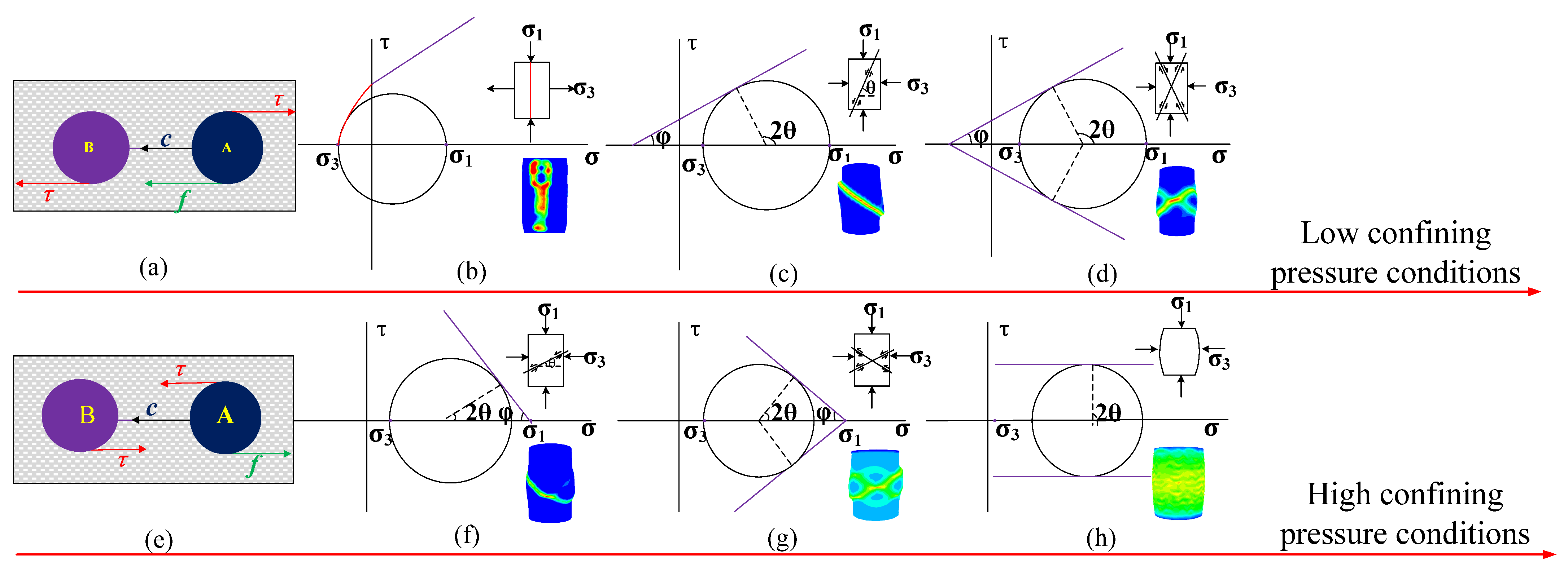
As shown in Figure 1, under low confining pressure (k < 3.7), increasing confining pressure drives the fracture mode to evolve from high-angle shear fractures to high-angle conjugate fractures, with fractures exhibiting extensional characteristics and shear failure angles greater than 45°. In contrast, under high confining pressure (k > 3.7), increasing confining pressure induces a transition from low-angle shear fractures to low-angle conjugate fractures, accompanied by compactional fracture properties and shear failure angles less than 45°. In this condition, compaction dominates under high confining pressure, facilitating the formation of low-angle shear fractures. Further increases in confining pressure lead to the development of low-angle conjugate shear fractures. When confining pressure becomes extremely high, rocks undergo ductile deformation, yielding no macroscopic fractures or forming dispersed microcracks that develop into fracture networks.

Figure 1. Evolution of rock fracture modes with increasing confining pressure. At low confining pressure (a–d): ideal stress model of rock (a), the deformation mechanism of high-angle splitting fracture (b), high-angle shear fracture (c), and high-angle conjugate shear fracture (d); at high confining pressure (e–h): ideal stress model of rock (e), the deformation mechanism of low-angle shear fracture (f), low-angle conjugate shear fracture (g), and plastic deformation (h). The colors in the rock sample represent the strain distribution pattern, and the areas where strain is concentrated are the parts of the rock sample that are prone to developing cracks (modified according to Wang et al., 2025 [43]).

Figure 1. Evolution of rock fracture modes with increasing confining pressure. At low confining pressure (a–d): ideal stress model of rock (a), the deformation mechanism of high-angle splitting fracture (b), high-angle shear fracture (c), and high-angle conjugate shear fracture (d); at high confining pressure (e–h): ideal stress model of rock (e), the deformation mechanism of low-angle shear fracture (f), low-angle conjugate shear fracture (g), and plastic deformation (h). The colors in the rock sample represent the strain distribution pattern, and the areas where strain is concentrated are the parts of the rock sample that are prone to developing cracks (modified according to Wang et al., 2025 [43]).

(b)

The control mechanism of Young’s modulus on fracture modes

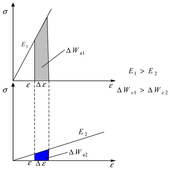
There is a close relationship between Young’s modulus E and the mechanical deformation of rock, which can be regarded as an elastomer. Under the stress loading condition, the elastic strain energy W_e is continuously stored during the compression process of the rock, and when W_e reaches the bonding energy W_b between particles inside the rock, random fractures are produced, the elastic energy is released at the same time, the rock enters into the yielding process, and the fractures expand and penetrate to eventually form macroscopic ruptures. As shown in Figure 2, the cumulative elastic strain energy per unit strain ΔW_e is a key energy parameter governing the fracture development mode of rocks under stress loading. The greater the Young’s modulus E, the higher the ΔW_e, leading to a more significant increase in the amplitude of stored elastic strain energy W_e.

Figure 2. Comparison of elastic strain energy accumulation per unit strain for different sizes of Young’s modulus.

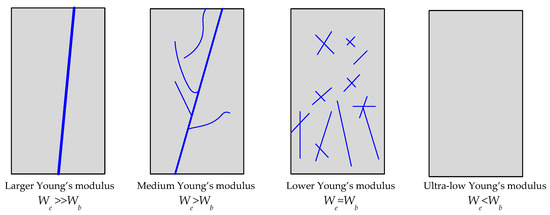
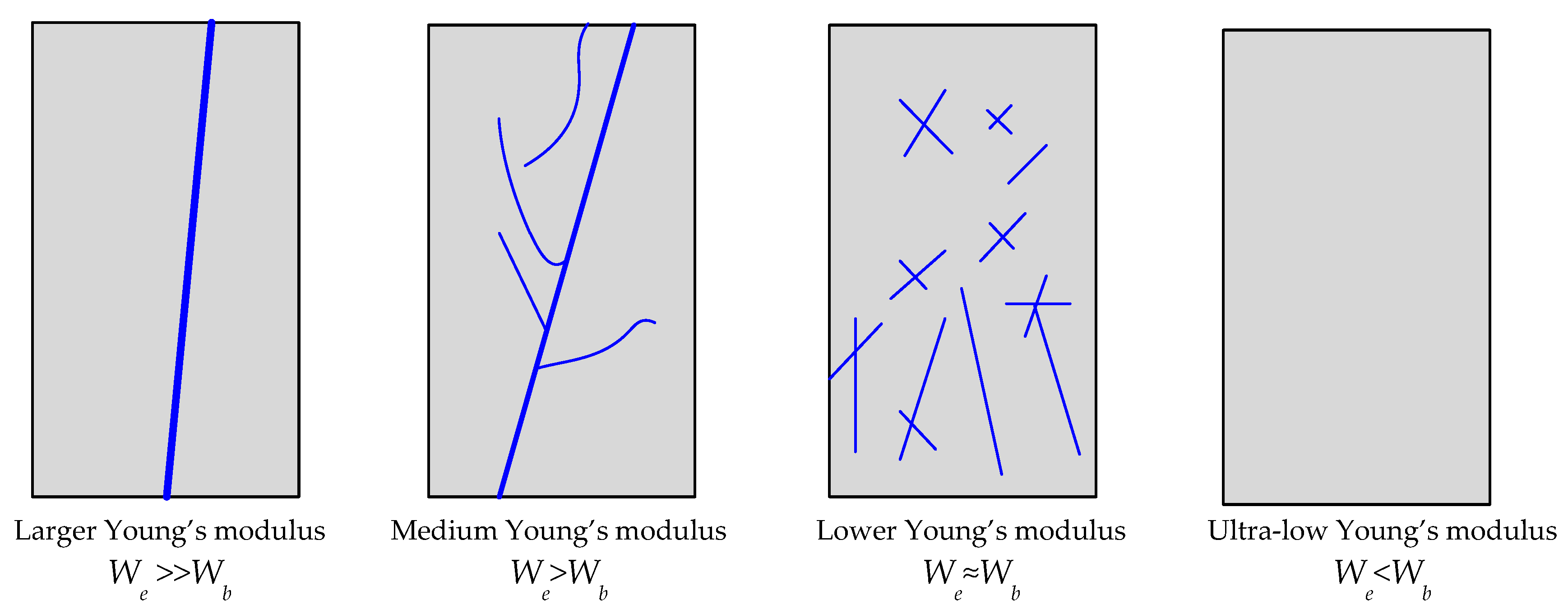
For rocks with a large modulus of elasticity E, the elastic strain energy accumulation per unit strain ΔW_e is large, as shown in Figure 3. When yield is reached, and W_e >> W_b, fractures are formed inside the rock, the energy is instantly released along the first fracture formed, inducing the expansion of the crack to form a macroscopic rupture, which tends to have a single fracture. For rocks with a medium modulus of elasticity E, the elastic strain energy accumulation per unit strain ΔW_e is not very large. When it reaches yield and W_e > W_b, fractures are formed inside the rock, and the energy is released along the first formed fracture, but it does not reach the energy condition to make the fracture expand to form a macro rupture, resulting in other random fractures having the opportunity to expand before the macro rupture of the rock. Finally, the extended fractures are connected to form a macro rupture, so the formation of the macro main fracture is accompanied by other fractures branching around it. For rocks with a small elastic modulus E, the elastic strain energy accumulation per unit strain ΔW_e is very small. When it reaches yield, and W_e ≈ W_b in the yielding process to generate random fractures, due to the elastic strain energy W_e being small, each fracture extension is very weak. Finally, dispersed fractures are formed, and macroscopically, there is no obvious penetration of the main fractures. When Young’s modulus continues to decrease, at this time, the elastic strain energy accumulation per unit strain ΔW_e is very small, with limited strain range energy. With the existence of W_e < W_b, no cracking occurs within the rock, which instead undergoes plastic deformation.

Figure 3. Schematic diagram of different fracture patterns developed with different Young’s moduli.

(c)

Mechanical deformation modulus describing the variability of rock fracture modes

Based on the study of the control mechanism of rock fracture modes by the intrinsic mechanical properties of rocks and external stress conditions, Young’s modulus parameters and differential stress coefficients are used to construct the deformation modulus used to describe the variability of rock fracture modes as in Equation (1).

$$E_F=f\left(E,{\displaystyle \frac{{\sigma }_3}{{\sigma }_1-{\sigma }_3}}\right)$$

(1)

The construct-based mechanical modulus needs to be considered to satisfy three conditions given by Equations (2)–(4).

$$f\left(E,{\displaystyle \frac{{\sigma }_3}{{\sigma }_1-{\sigma }_3}}\right)=E·g\left({\displaystyle \frac{{\sigma }_3}{{\sigma }_1-{\sigma }_3}}\right)$$

(2)

$${E·g\left({\displaystyle \frac{{\sigma }_3}{{\sigma }_1-{\sigma }_3}}\right)|}_{{\sigma }_{3=0}}=E$$

(3)

Since the deformation modulus describing the macroscopic fracture mode is characterized using Young’s modulus and stress conditions, when Young’s modulus approaches zero, or the confining pressure becomes extremely high, both cases indicate an absence of fracture development from the perspective of fracture evolution and are manifested mainly as plastic deformation. Therefore, from this perspective, the deformation modulus obtained under these two limiting conditions should be equal.

$$\underset{E\to 0}{\mathit{lim}}f\left(E,{\displaystyle \frac{{\sigma }_3}{{\sigma }_1-{\sigma }_3}}\right)=\underset{{\sigma }_3\to \mathrm{\infty }}{\mathit{lim}}f\left(E,{\displaystyle \frac{{\sigma }_3}{{\sigma }_1-{\sigma }_3}}\right)$$

(4)

Previous studies indicate that the influence of confining pressure on rock deformation and failure commonly exhibits a high sensitivity at low confinement and a tendency toward saturation at higher confinement. At low confining pressures, compliant defects within the rock are more readily and rapidly closed, such that the apparent stiffness and failure mode respond strongly to changes in confinement. As confining pressure further increases, these defects become progressively closed and stabilized, and the incremental effect of additional confinement on the elastic response and fracture development gradually weakens, resulting in a nonlinear trend that is “strong at first and then progressively levels off” [45,46]. Based on this mechanical rationale, the trial function is adopted:

$$E_F=E·e^{-{\displaystyle \frac{{\sigma }_3}{{\sigma }_1-{\sigma }_3}}}=E·e^{-{\displaystyle \frac{1}{k}}}$$

(5)

where $k={\displaystyle \frac{{\sigma }_1-{\sigma }_3}{{\sigma }_3}}$ is the differential stress coefficient [44].

When the Young’s modulus E is larger and the differential stress coefficient k is larger, then the deformation modulus E_F is larger, indicating that the rock is more likely to develop a single high-angle fracture after rupture, and the fracture is easy to expand. On the contrary, the smaller the deformation modulus E_F, the easier it is to form scattered cross fractures or the fracture networks, and the fractures are not easy to expand. When the deformation modulus E_F is very small, the rock undergoes plastic deformation, and it is not easy to produce fractures.

3. Evaluation Method of “Ternary Index”

(1)

Fracture Crack Index (FCI)

The initial formation of rock fractures begins with crack initiation, the difficulty of which is generally closely related to the tensile strength properties of the rock. The lower the tensile strength, the more easily the rock will crack. Therefore, define the rock fracture crack index FCI based on the tensile strength values tested in each formation.

$$FCI={\displaystyle \frac{T_{max}-T}{T_{max}-T_{min}}}$$

(6)

where T is the tensile strength of each formation, T_max is the maximum tensile strength in the formation, and T_min is the minimum tensile strength in the formation. The larger the index, the higher the level of fracture cracking in the formation relative to other formations, and the smaller the corresponding tensile strength.

(2)

Fracture Growth Index (FGI)

After the rock begins to crack, the fracture starts to grow. The ease with which these fractures grow is closely related to the rock’s fracture toughness. The greater the fracture toughness, the more difficult it is for the crack to grow. Define the rock fracture growth index FGI based on the fracture toughness strength values tested in each formation.

$$FGI={\displaystyle \frac{K_{max}-K}{K_{max}-K_{min}}}$$

(7)

where K is the fracture toughness of each oil formation, K_max is the maximum fracture toughness in the oil formation, and K_min is the minimum fracture toughness in the oil formation. The larger the index, the higher the level of fracture extension of the oil formation relative to other oil formations, and the smaller the corresponding fracture toughness strength.

(3)

Fracture Mode Index (FMI)

Based on the mechanical deformation modulus (E_F) tested for each oil interval, the fracture mode index FMI is defined.

$$FMI={\displaystyle \frac{E_F-E_{Fmin}}{E_{Fmax}-E_{Fmin}}}$$

(8)

where E_F is the value of the mechanical deformation modulus of each formation, E_Fmax is the maximum mechanical deformation modulus in the formation, and E_Fmin is the minimum mechanical deformation modulus in the formation.

(4)

“Ternary index” evaluation model

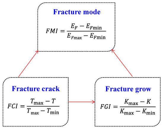
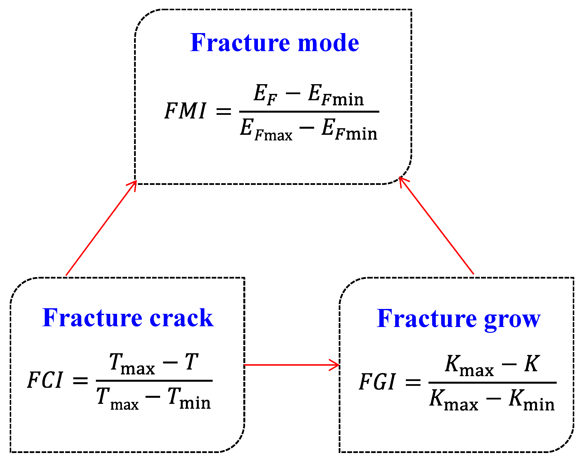
Rock fracture is a complex mechanical process that can usually be divided into three main stages: the fracture crack stage, the fracture growth stage, and the fracture mode formation stage. These three stages are interrelated and together determine the rupture behavior of rocks under stress. The crack level is the critical stress state at which fractures begin to develop in a rock under stress. Fracture growth is the process that determines the further expansion of the fractures in the rock under stress after fracture cracks. Fracture mode refers to the morphology and distribution characteristics of the fracture network formed in the process of rock rupture. Therefore, considering the influence of shale mechanical properties on fracture crack, fracture growth and fracture development mode, a ternary evaluation model of shale fracture development characteristics based on the variability of shale mechanical properties is established (Figure 4).

Figure 4. Ternary evaluation model of mechanical deformation of Gulong Shale: “cracking–growth–seam network mode”.

4. Experiment

4.1. Experimental Methods

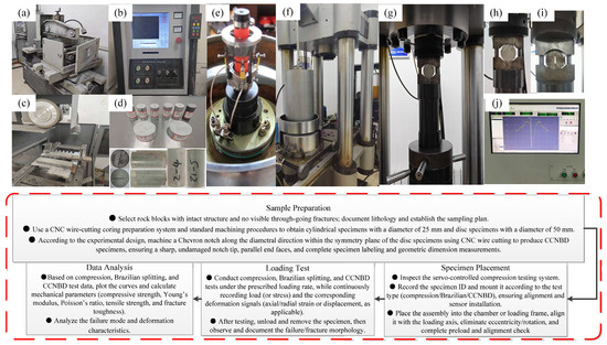
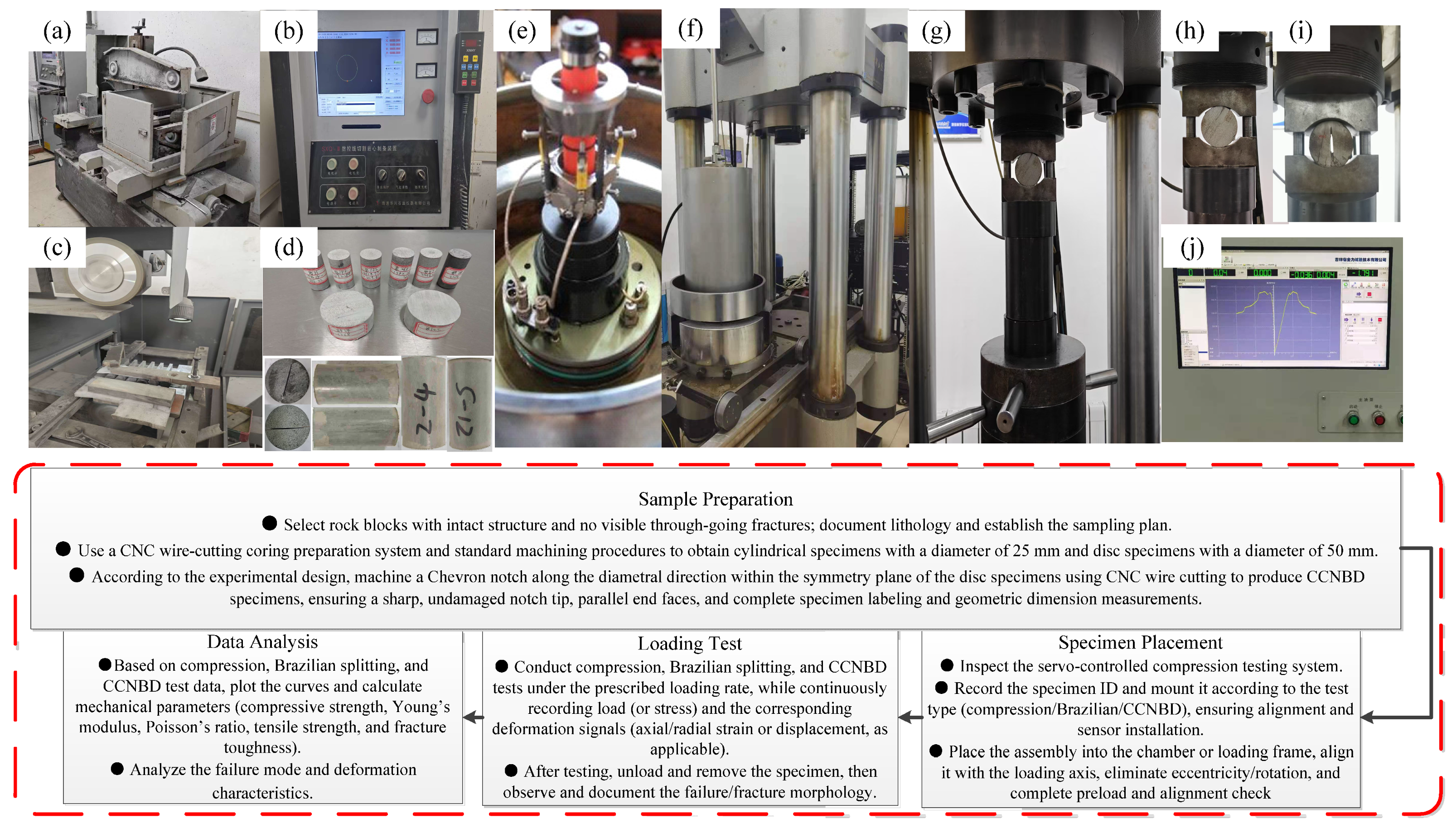
Taking Gulong Shale as an example, the Gulong Shale was hydraulically fractured in horizontal wells, and samples were systematically collected along vertical bedding planes at different depths, covering all oil intervals from Q1 to Q9. Based on the collected cores, standard specimens for triaxial compression, Brazilian splitting, and fracture-toughness tests were prepared using a CNC wire-cutting coring preparation system (Figure 5a–c), as shown in Figure 5d. A total of 100 samples were tested, yielding key mechanical parameters including Young’s modulus, Poisson’s ratio, compressive strength, tensile strength, and fracture toughness.

Figure 5. Integrated experimental procedure and instrumentation for triaxial compression, Brazilian splitting, and CCNBD fracture-toughness tests: (a–c) CNC wire-cutting core preparation system; (d) laboratory specimens; (e,f) triaxial compression testing system; (g–i) CCNBD and Brazilian splitting experimental platform; (j) LabVIEW software interface.

(1)

Triaxial Compression Experiment

The experimental equipment utilizes the TAW-2000 microcomputer-controlled electrohydraulic servo rock triaxial testing machine, manufactured by Changchun City Chaoyang Test Instrument Co., Ltd. in Changchun, China. To compare the mechanical properties of different types of rocks, specimens are designed to have identical size and shape. It has been observed that under typical peri-compression conditions, the diameter of cylindrical specimens typically ranges from 20 to 60 mm, with a height-to-diameter ratio of 2 to 3, minimizing dimensional effects. The axial and radial deformation of the specimen is measured using an induction gauge, while the axial load is dynamically monitored by a pressure transducer. The experimental equipment and measuring instruments are depicted in Figure 5e,f.

The specimen is processed into a core with a diameter of approximately 25 mm, and the ratio of the specimen’s height to its diameter is roughly 2.0 to 2.5 for standard cylindrical specimens. The unevenness of the two end surfaces of the specimen is less than 0.05 mm, the error in height and diameter is less than 0.3 mm, and the maximum deviation of the end face perpendicular to the specimen’s axis is less than 0.25°.

Estimate the effective confining pressure conditions of the core, given the static rock conditions, for the actual burial depth at which the core is located.

$${\sigma }_3^{\prime }={\int }_0^z\rho \left(z\right)gdz-\alpha P\left(z\right)$$

(9)

where P is the formation pressure, and z is the actual burial depth of the core. α denotes the Biot coefficient, which characterizes the degree to which pore-fluid pressure contributes to the effective stress acting on the rock skeleton. In this study, $\alpha$ was assumed to be 1.0 for all samples. The formation pressure $P\left(\mathrm{z}\right)$ at depth $\mathrm{z}$ was estimated under normal hydrostatic conditions.

Experiments were conducted to obtain the complete stress–strain curves of the rock samples throughout the destruction process, as well as various rock mechanical parameters, including compressive strength, Young’s modulus, Poisson’s ratio and post-peak softening modulus.

(2)

Tensile Strength Experiment

The tensile strength of rock is the maximum stress it can endure under tensile conditions. Owing to the simplicity of the Brazilian splitting test, the measured tensile strength is very similar to that obtained from the direct tensile method, making this technique commonly employed to ascertain the tensile strength of rocks.

According to the ISRM-recommended method for determining the tensile strength of rock materials [47], specimens were extracted from the core and fashioned into disc-shaped standard specimens with a diameter of approximately 50 mm. The ratio of the specimen’s height to its diameter was maintained between 0.5 and 1. The parallelism error between the two end surfaces was kept below 0.02 mm, and the surface roughness Ra was less than 1.6 μm. The edges were polished to prevent chipping during loading. The disk’s axis was oriented perpendicular to the loading direction, with a deviation not exceeding 0.1°.

The fundamental principle of the splitting method is based on the theoretical solution for the elasticity of a disk under opposing compressive forces. The maximum tensile stress that acts at the center of the specimen at the moment of its failure is:

$${\sigma }_{\mathrm{t}}={\displaystyle \frac{2P}{\pi dt}}$$

(10)

σ_t—Maximum tensile stress at the center of the specimen, i.e., tensile strength, MPa.

P—The ultimate pressure at the destruction of the sample, in Newtons (N).

dt—The diameter and thickness of the pressurized disk, in millimeters (mm).

The experimental platform was constructed using the TAW-2000 microcomputer-controlled electro-hydraulic servo rock triaxial testing machine, as depicted in Figure 5g,h. The displacement load was applied axially at a rate of 0.005 m per minute until complete destruction occurred. Experimental rock samples were utilized to test the pressure–displacement curve and to determine the fracture pressure, as well as to calculate the rock’s tensile strength.

(3)

Fracture Toughness Experiment

A herringbone-notched Brazilian disk specimen (CCNBD) was utilized to evaluate the fracture toughness of the rock. Diamond saw blades were employed to cut the rock into disk shapes, ensuring that the parallelism error of the end faces was less than 0.02 mm. The central herringbone notch was crafted using a wire-cutting machine, with the notch width being less than 0.1 mm. The herringbone notch needed to be symmetrical relative to the loading diameter, with a deviation not exceeding 1% of the diameter. Additionally, the notched surface exhibited a roughness of less than 1.6 μm. ${\alpha }_0$, ${\alpha }_1$, and B are the three basic geometric parameters of the CCNBD test, where ${\alpha }_0$ represents the initial fracture length of the specimen, ${\alpha }_1$ is the maximum notch length of the specimen, B is the thickness of the specimen, and α is the critical crack length.

All geometric parameters of the specimen are converted to dimensionless parameters using the radius and diameter of the rock sample. The conversion relationships are as follows:

$$\begin{array}{l}{\alpha }_0=a_0/R\\ {\alpha }_1=a_1/R\\ {\alpha }_B=B/R\end{array}$$

(11)

In order to ensure that the test results are valid, the selected parameters must fulfill the following restrictions [47].

$$\{\begin{array}{c}{\alpha }_1\ge 0.4\hfill \\ {\alpha }_1\ge {\alpha }_B/2\hfill \\ {\alpha }_B\le 1.04\hfill \\ {\alpha }_1\le 0.8\hfill \\ {\alpha }_B\ge 1.1729·{\alpha }_1^{1.6666}\hfill \\ {\alpha }_B\ge 0.04\hfill \end{array}$$

(12)

The fracture toughness of the CCNBD specimen is calculated as:

$$K_{IC}={\displaystyle \frac{P_{max}}{B·\sqrt{D}}}·Y_{min}^{\ast }$$

(13)

K_IC—Type I fracture toughness value, MPa·m^1/2.

P_max—Maximum destructive load value, kN.

D—Specimen diameter, cm.

B—Specimen thickness, cm.

Y*_min—Dimensionless critical stress intensity factor of the specimen, which is determined solely by the geometric parameters ${\alpha }_0$, ${\alpha }_1$ and ${\alpha }_{\mathrm{B}}$ of the rock sample. (In this paper, Y*_min utilizes the stress intensity factor recalibrated by Z. Q. Wang et al. 2013 [48].)

The experimental platform is constructed based on the TAW-2000 microcomputer-controlled electro-hydraulic servo rock three-axis testing machine, as depicted in Figure 5g,i. Specimens were diametrally loaded parallel to the chevron notch orientation under concentrated forces, using a constant displacement control mode. The loading rate was regulated by a loading-point displacement velocity of 0.5 mm/min. Load and deformation data were automatically recorded at discrete time intervals through the test frame’s integrated servo-control system software. The lower loading rate in the experiment is not only beneficial for the stable expansion of the fracture along the prefabricated fracture surface but also for the full development of the nonlinear fracture process zone at the crack tip and for the measurement of a more effective fracture toughness value.

4.2. Experimental Results

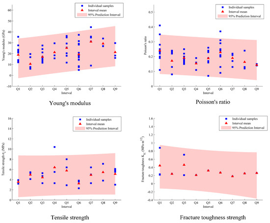
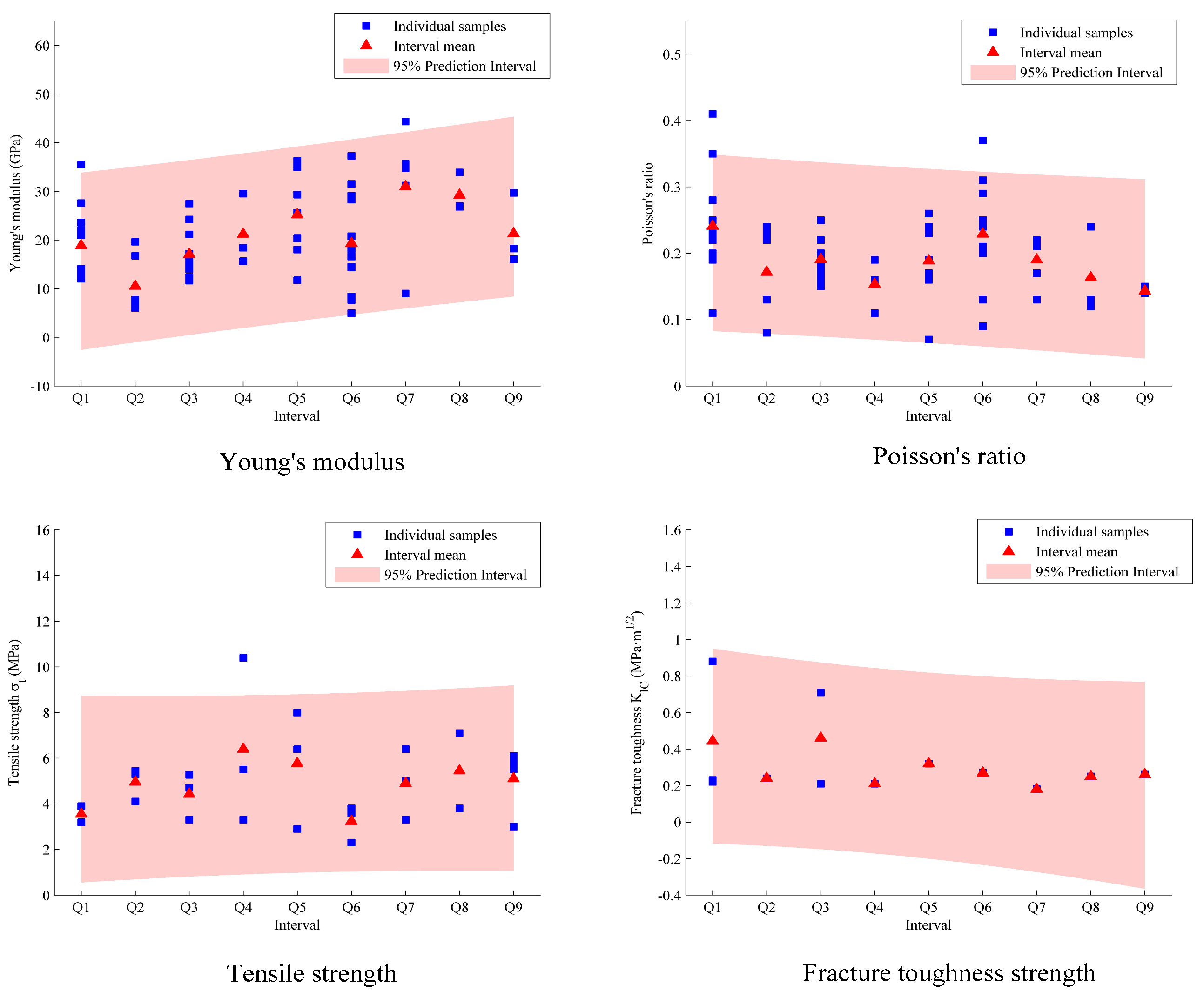
Through the above series of experiments, the mechanical deformation parameters and strength parameters of different intervals of Gulong Shale were obtained, as shown in Table 2, Table 3 and Table 4. It should be noted that both the Brazilian splitting and fracture-toughness tests require disc-shaped specimens, and pre-existing cracks need to be fabricated for fracture toughness specimens. Due to such stringent preparation requirements, it is difficult to meet the specifications during the preparation of strongly heterogeneous shale. Consequently, the number of valid specimens is 26 for tensile strength tests and 13 for fracture toughness tests, both of which are far fewer than those for elastic parameter tests, introducing certain uncertainty in the subsequent comprehensive evaluation. Nevertheless, the scatter distributions of elastic parameters, tensile strength, and fracture toughness across the Q1–Q9 intervals (Figure 6) show that both the measured data points and the corresponding interval means generally fall within the prediction interval at the 95% confidence level, indicating that the tested specimens exhibit acceptable reliability and representativeness at the interval scale.

Table 2. Mechanical modulus parameters of shale at different intervals.

Interval	Sample Number	Well Number	Uniaxial Compressive Strength (MPa)	Young’s Modulus (GPa)	Poisson’s Ratio
Q1	1	rc1	101.2	23.58	0.19
	2		111.4	27.59	0.23
	3		154.2	35.46	0.28
	4	ws2	14.78	13.86	0.22
	5		62.46	12.05	0.35
	6	ws3	49.4	12.41	0.25
	7		95.4	22.1	0.2
	8		71.3	21	0.11
	9		79.1	13.3	0.22
	10		76.7	14.08	0.41
	11		51.9	12.04	0.19
Q2	12	rc1	86.7	6.02	0.23
	13		90.6	6.06	0.22
	14		35.5	7.01	0.13
	15		24.9	7.72	0.08
	16		58.8	16.77	0.13
	17		64.8	19.62	0.24
Q3	18	rc3	100.9	17.19	0.2
	19		97	14.88	0.19
	20		81.8	14.02	0.19
	21		159.7	24.22	0.22
	22		98.7	15.67	0.15
	23		73.1	12.41	0.16
	24		33.6	11.63	0.18
	25		69.3	12.03	0.2
	26		114.5	16.66	0.25
	27		139.5	21.14	0.19
	28	rc1	153.5	27.5	0.17
Q4	29	rc3	97.1	15.68	0.11
	30		115.6	18.42	0.16
	31	rc1	172.9	29.5	0.19
Q5	32	rc3	115.9	18.01	0.17
	33		134.5	20.32	0.07
	34		52.6	11.74	0.23
	35	rc1	168.6	36.27	0.24
	36		160.1	34.9	0.26
	37		148.2	29.3	0.16
	38		131.8	25.6	0.19
Q6	39	rc3	133.3	20.79	0.24
	40		86	18.12	0.09
	41		91.9	16.59	0.2
	42	rc1	145.6	31.53	0.21
	43	ws4	72.66	14.5	0.21
	44		90.27	14.39	0.29
	45		67.68	8.4	0.31
	46		73.94	7.67	0.37
	47		15.7	5	0.13
	48	xk1	103.3	29.1	0.21
	49		85.9	28.3	0.24
	50	ws3	172.3	37.28	0.25
Q7	51	rc1	109.4	9	0.17
	52		95.4	44.34	0.13
	53	rc4	174	34.8	0.22
	54		164	35.66	0.22
	55		193	31.2	0.21
Q8	56	rc2	147.6	27	0.12
	57		145.4	26.8	0.13
	58	rc4	178	33.9	0.24
Q9	59	rc1	80.52	16.04	0.14
	60	rc2	75.97	18.24	0.15
	61	xk2	134.16	29.69	0.14

Table 3. Brazilian tensile strength (BTS) results of shale at different intervals.

Interval	Sample Number	Well Number	Tensile Strength/σt (MPa)
Q1	1	rc3	3.2
	2	rc2	3.9
	3	rc1	3.5
Q2	4	rc2	4.1
	5	ws1	5.3
Q3	6	rc3	3.3
	7	rc1	2
	8	rc2	4.7
Q4	9	rc3	3.3
	10	rc2	5.5
	11	ws1	10.4
Q5	12	rc3	8
	13	rc2	6.4
	14	ws1	2.9
Q6	15	rc3	3.6
	16	rc2	3.8
	17	ws4	2.3
Q7	18	rc2	5
	19	xk1	3.3
Q8	20	rc2	7.1
	21	ws1	3.8
Q9	22	rc3	3
	23	rc1	5.45
	24	rc2	5.8
	25	ws1	6.1
	26	xk2	4.39

Table 4. Experimental fracture toughness results for shale at different intervals.

Interval	Sample Number	Well Number	Fracture Toughness Strength/KIC (MPa·m1/2)
Q1	1	rc1	0.88
	2	xk3	0.23
	3	rc2	0.22
Q2	4	rc2	0.24
	5	xk1	/
Q3	6	rc3	0.71
	7	rc2	0.21
Q4	8	rc2	0.21
Q5	9	rc2	0.32
Q6	10	rc2	0.27
Q7	11	rc2	0.18
Q8	12	rc2	0.25
Q9	13	rc2	0.26

Notes: “/” indicates that a valid K_IC value was not obtained for the specimen; therefore, Q2 contains only one valid fracture-toughness measurement.

Figure 6. Interval–wise distributions of elastic parameters, tensile strength and fracture toughness across Q1–Q9 (95% prediction intervals).

(a)

Deformation Modulus Characteristics

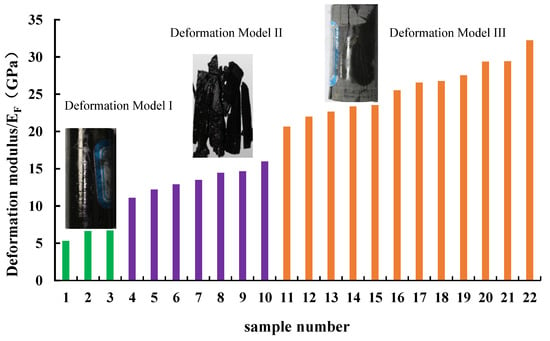
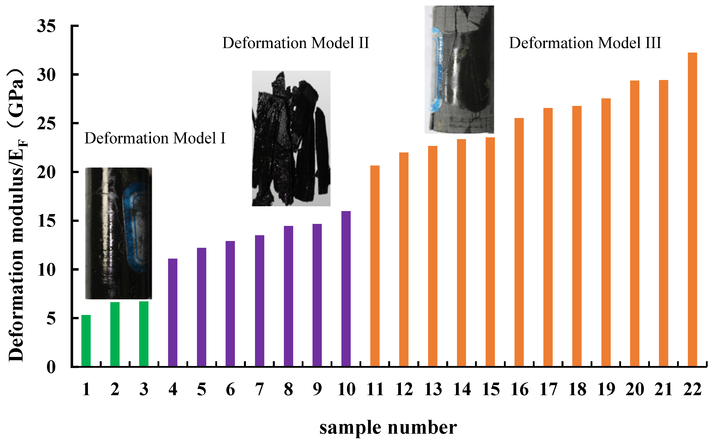
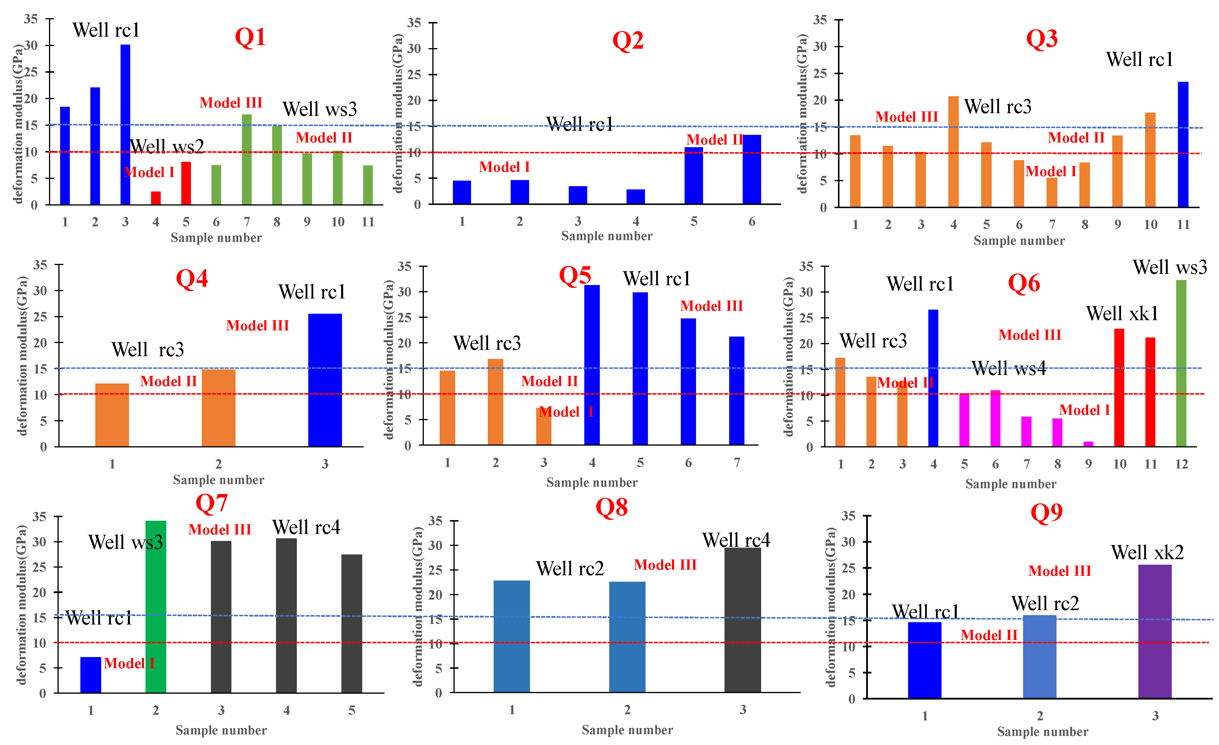
Based on the mechanical parameters of different layers, the average mechanical deformation modulus (E_F) (Table 2) for each well is obtained. Based on the statistical analysis of rock fracture mode differences using the shale dataset from the Gulong area, the shale deformation characteristics can be classified into three deformation models (Figure 7). Deformation model I exhibits a deformation modulus of less than 10 GPa (E_F < 10 GPa). This model indicates that the rock has minimal macroscopic ruptures and small fracture apertures, with a limited capacity to generate fractures. Deformation model II possesses a deformation modulus ranging from 10 GPa to less than 15 GPa (10 GPa < E_F < 15 GPa). Within this model, strain tends to disperse readily under stress, and the resulting dispersed ruptures often evolve into a complex network of low-angle fractures. Deformation model III has a deformation modulus exceeding 15 GPa (E_F > 15 GPa). In this model, strain is concentrated, facilitating the development of a network of fractures with high angles, creating through-going fractures. Notably, the boundaries between the three deformation models were determined from the fracture-mode statistical analysis of the present dataset and should therefore be regarded as dataset-specific unless independently validated.

Figure 7. Schematic diagram of fracture development models in different deformation modes.

(b)

Tensile Strength Characteristics

Rock tensile strength is an important parameter that describes the resistance to fracture. The lower the tensile strength, the easier it is for a fracture to initiate. Conversely, the higher the tensile strength, the more difficult it is to initiate a fracture. A total of 26 Brazilian split test samples were conducted on the Q1 to Q9 interval (Table 3), with overall tensile strength distributed between 2 MPa and 10.4 MPa. The tensile strength distribution shows obvious variations among different intervals. The Q1 interval strength ranges from 3.2 MPa to 3.9 MPa with an average strength of approximately 3.53 MPa; the Q2 interval ranges from 4.1 MPa to 5.3 MPa with an average of approximately 4.7 MPa; the Q3 interval ranges from 3.3 MPa to 4.7 MPa with an average of approximately 3.33 MPa; the Q4 interval ranges from 3.3 MPa to 10.4 MPa with an average of approximately 6.4 MPa; the Q5 interval ranges from 2.9 MPa to 8 MPa with an average of approximately 5.77 MPa; the Q6 interval ranges from 2.3 MPa to 3.8 MPa with an average of approximately 3.23 MPa; the Q7 interval ranges from 3.3 MPa to 5 MPa with an average of approximately 4.15 MPa; the Q8 s interval ranges from 3.8 MPa to 7.1 MPa with an average of approximately 5.45 MPa; and the Q9 interval ranges from 3 MPa to 6.1 MPa with an average of approximately 4.95 MPa. It should be pointed out that due to the limited number of samples, the above-average values are mainly used to characterize the relative differences in strength levels of each interval and provide a data basis for subsequent quantitative evaluation. Their statistical representativeness is limited and may not be sufficient to reflect the true overall mean value of the corresponding interval.

(c)

Fracture Toughness Characteristics

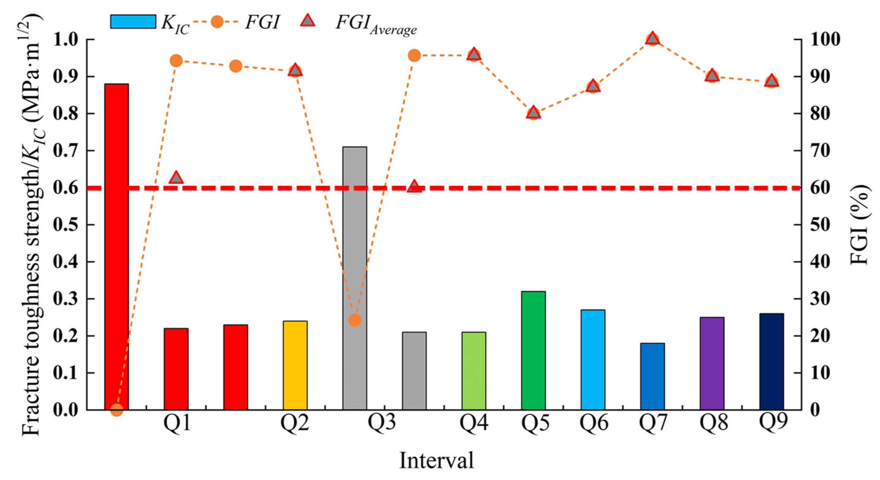
Fracture toughness is a critical parameter that characterizes fracture propagation in rocks. A lower value indicates easier fracture extension, whereas a higher value implies reduced propagability. Through conducting 12 tests of shale fracture toughness strength (perpendicular to bedding direction), the fracture toughness strength of each well was obtained (Table 4). Overall, the fracture toughness values of Q1–Q9 oil intervals are relatively small, with the fracture toughness K_IC of most samples concentrated between 0.2 and 0.3 MPa·m¹/². Among them, the K_IC of samples from Q1 and Q3 intervals are more dispersed; the K_IC of Q1 ranges between 0.22 and 0.88 MPa·m¹/², while the K_IC of Q3 ranges between 0.21 and 0.71 MPa·m¹/².

5. Fracability Evaluation Based on the Ternary Index Method

Based on the experimental results, the fracture crack, fracture growth, and fracture mode indices (Table 5) were calculated using the aforementioned formula to evaluate the mechanical property variations of the Gulong Shale. It should be emphasized that although the specimens were taken from different wells and certain inter-well differences may exist, the comparative analysis in this study focuses primarily on stratigraphic intervals. Differences between wells within the same interval are insignificant and generally do not affect the overall comparison results or ranking among intervals. Meanwhile, the thresholds adopted for index classification and model categorization are determined based on the fracture mode characteristics observed in the tested samples.

Table 5. Mechanical properties table of different oil intervals in different wells.

Interval	Well Number	Tensile Strength		Fracture Toughness Strength		Deformation Modulus
		Strength/MPa	FCI%	Strength/MPa·m1/2	FGI%	Modulus/GPa	Deformation Model	FMI%
Q1	rc1	3.5	82.14	0.88	0.00	23.54	III	67.69
	ws2	/	/	/	/	5.31	I	0.00
	ws3	/	/	/	/	11.09	II	21.46
	rc3	3.2	85.71	/	/	/	/	/
	rc2	3.9	77.38	0.22	94.29	/	/	/
	xk3	/	/	0.23	92.86	/	/	/
Q2	rc1	/	/	/	/	6.61	I	16.92
	rc2	4.1	75.00	0.24	91.43	/	/	/
	ws1	5.3	60.71	/	/	/	/	/
	xk1	/	/	/	/	/	/	/
Q3	rc3	3.3	84.52	0.71	24.29	12.19	II	25.55
	rc1	2	100.00	/	/	23.36	III	67.03
	rc2	4.7	67.86	0.21	95.71	/	/	/
Q4	rc3	3.3	84.52	/	/	13.47	II	30.30
	rc1	/	/	/	/	25.52	III	75.05
	rc2	5.5	58.33	0.21	95.71	/	/	/
	ws1	10.4	0.00	/	/	/	/	/
Q5	rc3	8	28.57	/	/	12.89	II	28.15
	rc1	/	/	/	/	26.76	III	79.65
	rc2	6.4	47.62	0.32	80.00	/	/	/
	ws1	2.9	89.29	/	/	/	/	/
Q6	rc3	3.6	80.95	/	/	14.47	II	34.01
	rc1	/	/	/	/	26.55	III	78.87
	ws4	2.3	96.43	/	/	6.69	I	5.12
	xk1	/	/	/	/	21.99	III	61.94
	ws3	/	/	/	/	32.24	III	100.00
	rc2	3.8	78.57	0.27	87.14	/	/	/
Q7	rc1	/	/	/	/	20.64	I	56.93
	rc4	/	/	/	/	29.39	III	89.42
	rc2	5	64.29	0.18	100.00	/	/	/
	xk1	3.3	84.52	/		/	/	/
	ws1	/	/	/		/	/	/
Q8	rc2	7.1	39.29	0.25	90.00	22.67	III	64.46
	rc4	/	/	/	/	29.45	III	89.64
	ws1	3.8	78.57	/	/	/	/	/
Q9	rc1	5.45	58.93			14.67	II	34.76
	rc2	5.8	54.76	0.26	88.57	15.99	III	39.66
	rc3	3	88.10	/	/	/	/	/
	ws1	6.1	51.19	/	/	/	/	/
	xk2	4.39	71.55	/	/	27.56	III	82.62

5.1. Fracture Mode Characteristics

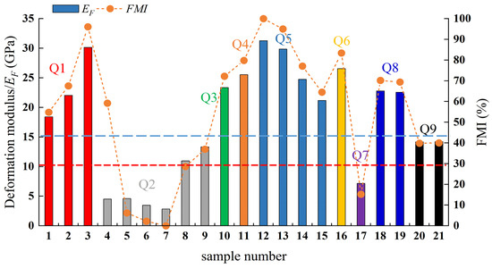
Figure 8 illustrates the rock mechanical deformation characteristics of different intervals within the same well (well rc1). As shown, in well rc1, Q2 and Q7 exhibit E_F generally below 10 GPa and FMI < 30%, classified as “low-modulus” shale. This type is less prone to forming through-fractures or possesses weak fracture-generating capacity. Q9 displays E_F between 10 GPa and 15 GPa, with 30% < FMI < 45%, termed “medium-modulus” shale. Strain tends to disperse, leading to distributed fracturing and the formation of complex fracture networks. For Q1, Q3, Q4, Q5, Q6, and Q8, E_F is generally greater than 15 GPa, classified as mechanical deformation model III with FMI > 45%. These are termed “high-modulus” shale, prone to developing open through-fractures with strong fracture-generating capacity.

Figure 8. Deformation modulus and FMI variations across intervals in Well rc1 (Note: The left y-axis shows the measured deformation modulus ${\mathrm{E}}_{\mathrm{F}}$ (GPa), the right y-axis shows the fracture mode index FMI (%), and different colors represent samples from different intervals).

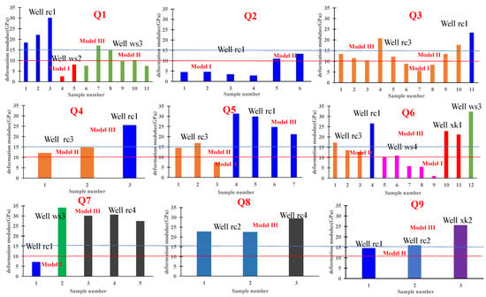
As shown in Figure 9, the distribution characteristics of E_F and FMI show significant differences among wells at the same interval, indicating strong heterogeneity in the study area. Q1, Q3, Q5, and Q6 intervals exhibit fracture development and deformation models I, II, and III. Q2 interval exhibits fracture development and deformation models I and II. Q4 and Q9 intervals exhibit fracture development models II and III. Q7 interval exhibits fracture development models I and III. Q8 interval exhibits fracture development model III.

Figure 9. Comparison of deformation modulus of different wells at the same interval.

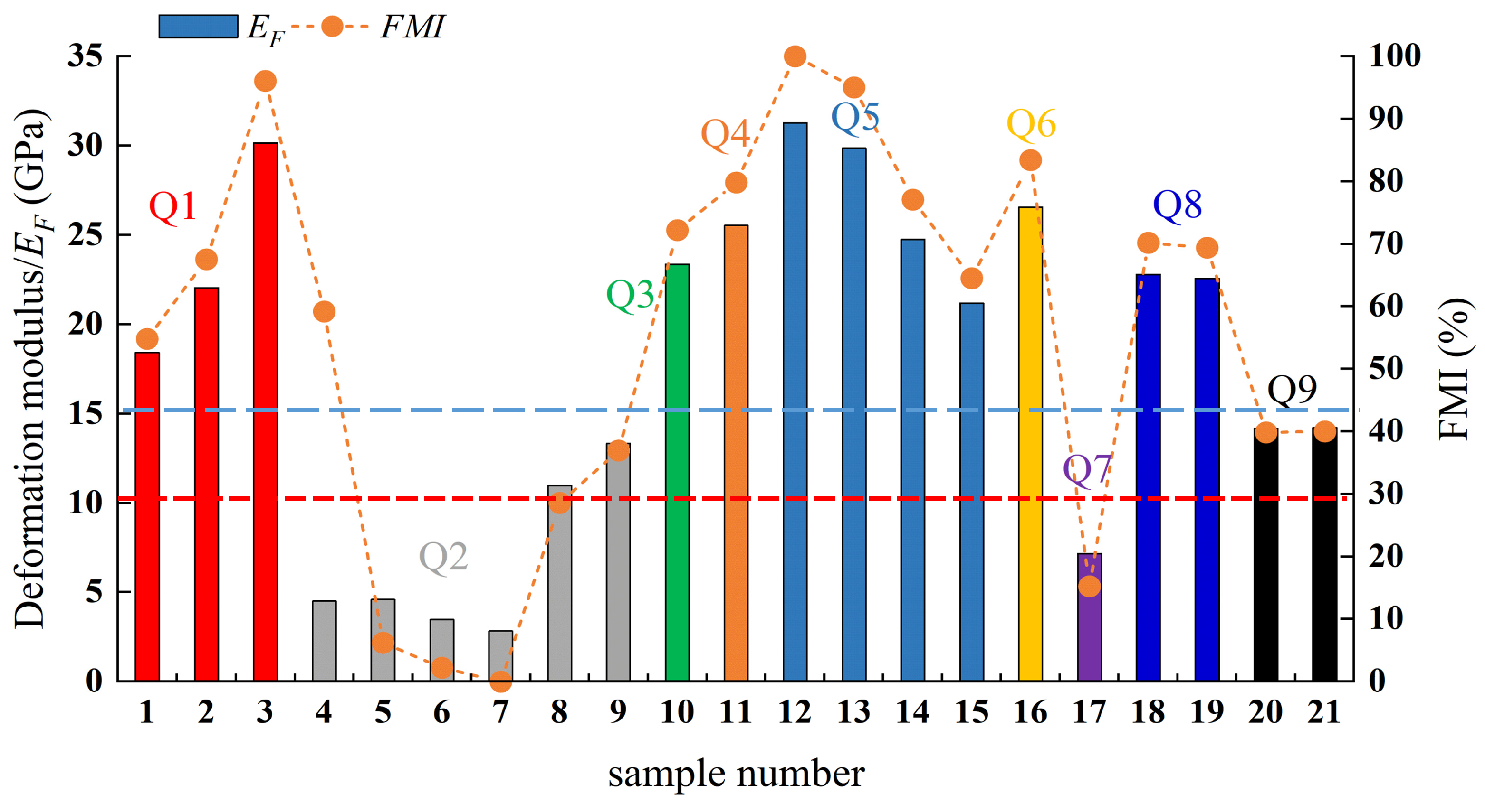
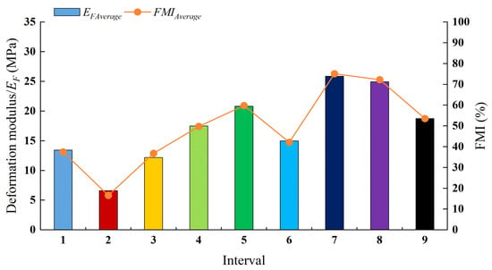
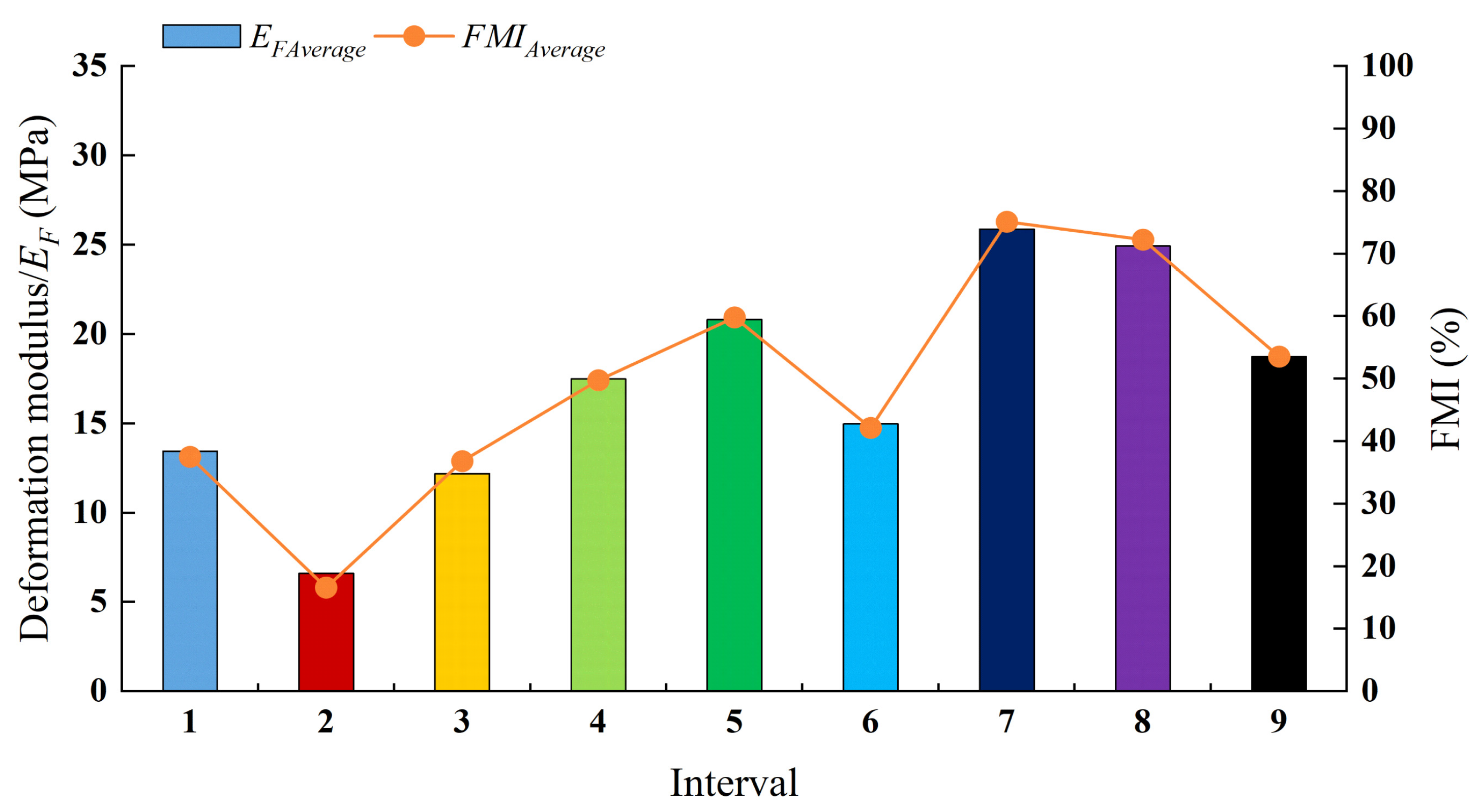
As shown in Figure 10 and Table 6, by obtaining the average values of E_F and FMI from different wells at the same interval and conducting lateral comparison: for Q2 (low-modulus shale), FMI_Average = 16.69% < 30%, E_FAverage = 6.61 GPa < 10 GPa, belonging to deformation mode I, which is not prone to forming through-going fractures or has weak cracking capacity; for Q1, Q3, and Q6 (medium-modulus shale), E_FAverage ranges from 10 GPa to 15 GPa, FMI_Average ranges from 30% to 45%, belonging to deformation mode II, which is prone to forming fracture network characteristics; and for Q4, Q5, Q7, Q8, and Q9 (high-modulus shale), EF_Average > 15 GPa, FMI_Average > 45%, belonging to deformation mode III, which is prone to developing high-angle through-going fractures.

Figure 10. Deformation modulus and FMI variation diagram for each interval.

Table 6. Interval-averaged values of FCI, FGI, and FMI for the Q1–Q9 intervals.

Interval	FCIaverage%	FGIaverage%	FMIaverage%
Q1	81.74 (wells = 3)	62.38 (wells = 3)	37.52 (wells = 3)
Q2	67.86 (wells = 2)	91.43 (wells = 1)	16.92 (wells = 1)
Q3	84.13 (wells = 3)	60.00 (wells = 2)	36.83 (wells = 2)
Q4	42.86 (wells = 3)	95.71 (wells = 1)	49.78 (wells = 2)
Q5	55.16 (wells = 3)	80.00 (wells = 1)	59.83 (wells = 2)
Q6	85.32 (wells = 3)	87.14 (wells = 1)	42.17 (wells = 5)
Q7	74.41 (wells = 2)	100.00 (wells = 1)	75.14 (wells = 2)
Q8	58.93 (wells = 2)	90.00 (wells = 1)	72.27 (wells = 2)
Q9	67.90 (wells = 5)	88.57 (wells = 1)	53.56 (wells = 3)

5.2. Fracture Crack Characteristics

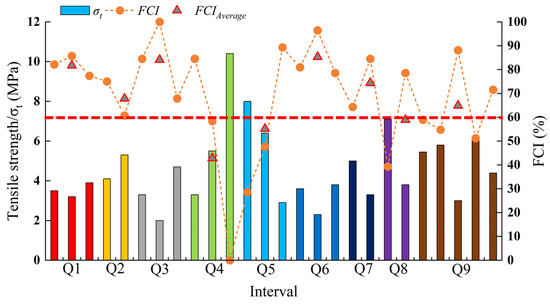
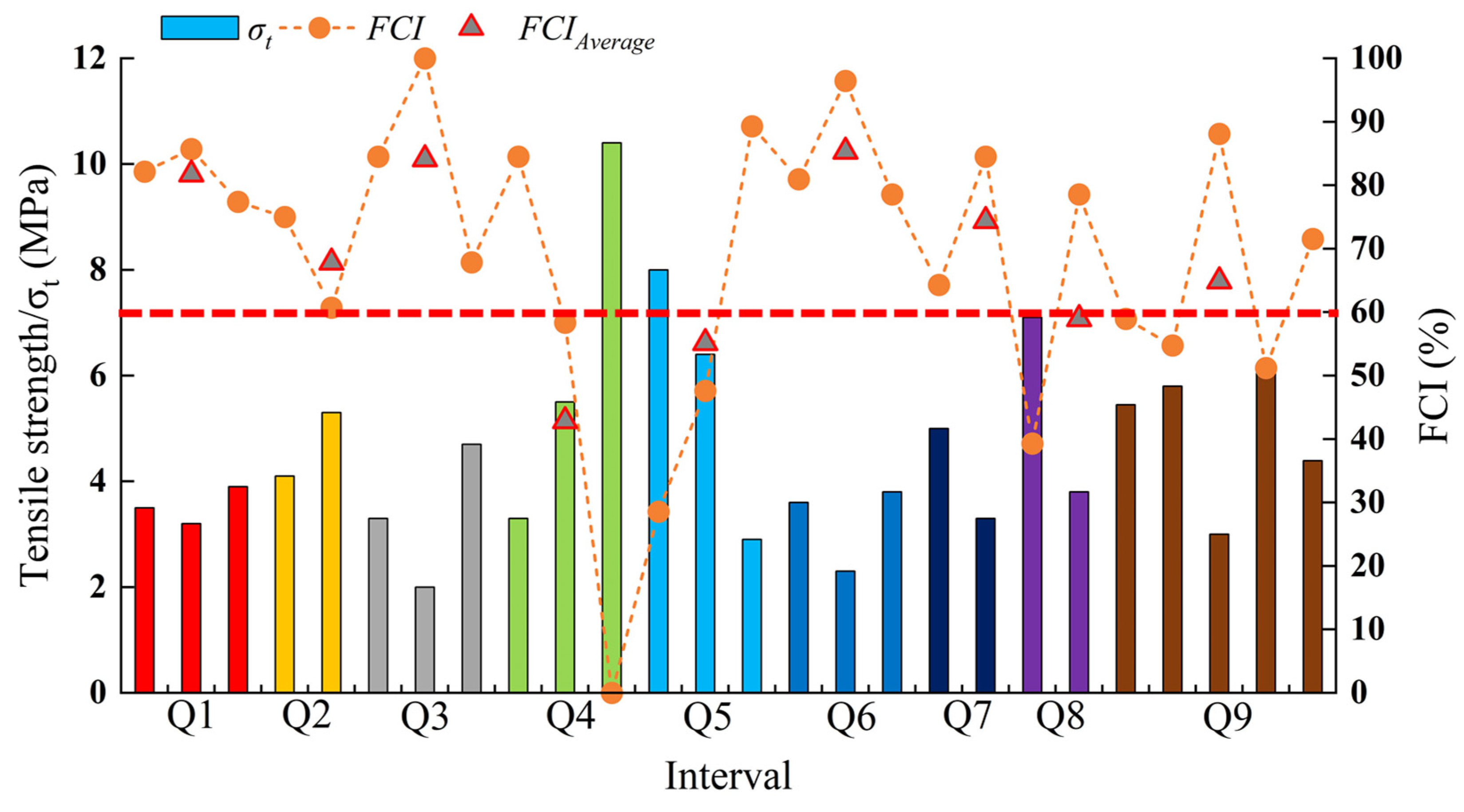
Based on the fracture crack index (FCI) evaluation of relative fracture initiation differences across the Q1-Q9 intervals (Figure 11 and Table 6), tensile strength distribution within the Q1-Q3, Q6, and Q9 intervals is uniform with low strength values. The overall FCI index exceeds 50%, indicating high susceptibility to cracking. The tensile strength distribution in Q4 (FCI between 0 and 80%), Q5 (FCI between 30 and 85%), and Q8 (FCI between 40 and 80%) shale intervals is dispersed, reflecting pronounced heterogeneity. Overall, the average fracturing indices across intervals, arranged from lowest to highest, are as follows: Q4 (FCI_Average = 42.86), Q5 (FCI_Average = 55.16), Q8 (FCI_Average = 58.93), Q9 (FCI_Average = 64.9), Q2 (FCI_Average = 67.86), Q7 (FCI_Average = 74.41), Q1 (FCI_Average = 81.74), Q3 (FCI_Average = 84.13), and Q6 (FCI_Average = 85.32). Shales with an average fracturing index FCI_Average > 60% are termed “low-tensile” shales, exhibiting easy fracturing and primarily distributed in the Q1-Q3, Q6, Q7, and Q9 intervals. Shales with FCI_Average < 60% are termed “high-tensile” shales, exhibiting difficult fracturing and primarily distributed in the Q4, Q5, and Q8 intervals.

Figure 11. Tensile strength and FCI variation chart for each oil interval (Note: The left y-axis shows the measured Brazilian tensile strength (${\mathsf{\sigma }}_{\mathrm{t}}$) (MPa), the right y-axis shows the fracture initiation index FCI (%), and different colors represent samples from different intervals).

5.3. Fracture Growth Characteristics

Based on the fracture growth index (FGI), the differences in relative fracture initiation degrees among Q1-Q9 intervals were evaluated (Figure 12 and Table 6). Overall, the average fracture growth index (FGI_Average) of each interval is greater than 60%, classifying them as “low toughness” shale, where fractures after initiation are prone to growth. Since one Q2 specimen has no valid fracture-toughness measurement (Table 4), the FGI_Average for Q2 was calculated based only on the single valid measurement. In comparison, the average fracture growth index (FGI_Average) of the Q2 and Q4-Q9 intervals is greater than 80%. The average fracture growth index of the Q1 (FGI_Average = 62.38%) and Q3 (FGI_Average = 60%) intervals is relatively low.

Figure 12. Fracture toughness and FGI variation diagram for each interval (Note: The left y-axis shows the measured fracture toughness ${\mathrm{K}}_{\mathrm{I}\mathrm{C}}$ (MPa·^1/2), and the right y-axis shows the fracture/growth/propagation capacity index FGI (%), different colors represent samples from different intervals).

6. Comprehensive Evaluation Results and Discussion

Based on the characteristics of the ternary indices of Gulong Shale, the fracability characteristics of Gulong Shale were classified into four types (Table 7): “low tensile–low toughness–low modulus” (Q2 interval), “low tensile–low toughness–medium modulus” (Q1, Q3, Q6 intervals), “low tensile–low toughness–high modulus” (Q7, Q9 intervals), and “high tensile–low toughness–high modulus” (Q4, Q5, Q8 intervals).

Table 7. Characteristics of four mechanical models of shale in the Gulong area.

Type of Mechanical Models	Interval	Mechanical Characteristics	Crack Mode
Low tensile–low toughness–low modulus	Q2	Easy to crack and expand, with small fracture apertures or poor fracturing capacity.
Low tensile–low toughness–medium modulus	Q1, Q3, Q6	Prone to cracking, prone to expansion, develops low-angle cross network.
Low tensile–low toughness–high modulus	Q7, Q9	Easy to crack and expand, develops a network of high-angle penetration joints.
High tensile–low toughness–high modulus	Q4, Q5, Q8	Difficult to crack, easy to expand, developing through-going fracture networks.

The Q2 interval (“low tensile–low toughness–low modulus” model) is mostly developed in the shallow reservoir section of the Gulong area, with moderate bedding cementation. Low tensile strength and low fracture toughness together reduce the difficulty of fracture cracking and growth, while the low deformation modulus corresponds to mechanical deformation model I. The macroscopic fracture characteristics of the rock are not significant, mostly forming micro-fracture networks with small apertures and poor connectivity. It is necessary to enhance the conductivity of micro-fractures and promote the competitive propagation of multiple fractures to achieve the expected results.

The Q1, Q3, and Q6 intervals (“low tensile–low toughness–medium modulus” model), where shale fractures in these intervals are prone to cracking and growth, have a medium deformation modulus (deformation model II), developing low-angle intersecting fractures and no obvious connected main fractures at the macroscopic level. During development, branch fracture propagation can be induced to enhance fracture network complexity.

The Q7 and Q9 intervals (“low tensile–low toughness–high modulus” model), as the core intervals of high-quality shale reservoirs in the Gulong area, predominantly consist of thick, high-quality reservoir sections with good internal homogeneity. Fractures are prone to cracking and grow easily, exhibiting a high deformation modulus (deformation model III). This facilitates the formation of wide, high-angle through-going main fractures accompanied by branch fractures, resulting in a high complexity of the fracture network.

The Q4, Q5, and Q8 intervals (“high tensile–low toughness–high modulus” model) exhibit high tensile strength that increases the difficulty of fracture cracks (low fracture density), while low fracture toughness promotes rapid fracture growth after initiation. With a high deformation modulus (deformation model III), they tend to form longitudinally penetrating extension fractures.

The evaluation results of the Gulong Shale based on the “ternary index” model are consistent with the actual fracability evaluation results. To further interpret interval-scale differences from the perspective of basic elasticity, we additionally calculated the Rickman-type brittleness index (BI) from Young’s modulus and Poisson’s ratio, where rocks with a higher Young’s modulus and a lower Poisson’s ratio are generally considered more brittle [37]. Rickman, focusing on the mechanical parameters of the Barnett shale in North America, proposed using the average of the normalized Young’s modulus and Poisson’s ratio as a brittleness index to quantify the relative brittleness of shale.

$$BI={\displaystyle \frac{1}{2}}\left({\displaystyle \frac{E-E_{min}}{E_{max}-E_{min}}}+{\displaystyle \frac{{\nu }_{max}-\nu }{{\nu }_{max}-{\nu }_{min}}}\right)$$

(14)

where E is Young’s modulus (GPa) and v is Poisson’s ratio (dimensionless); E_max and E_min are the maximum and minimum Young’s moduli of the dataset, and ν_max and ν_min are the maximum and minimum Poisson’s ratios. Previous studies summarizing the Rickman method have noted that BI > 40% can be regarded as indicating evident brittleness, while BI > 60% corresponds to very strong brittleness and is commonly used as an empirical engineering threshold [49].

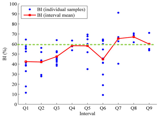
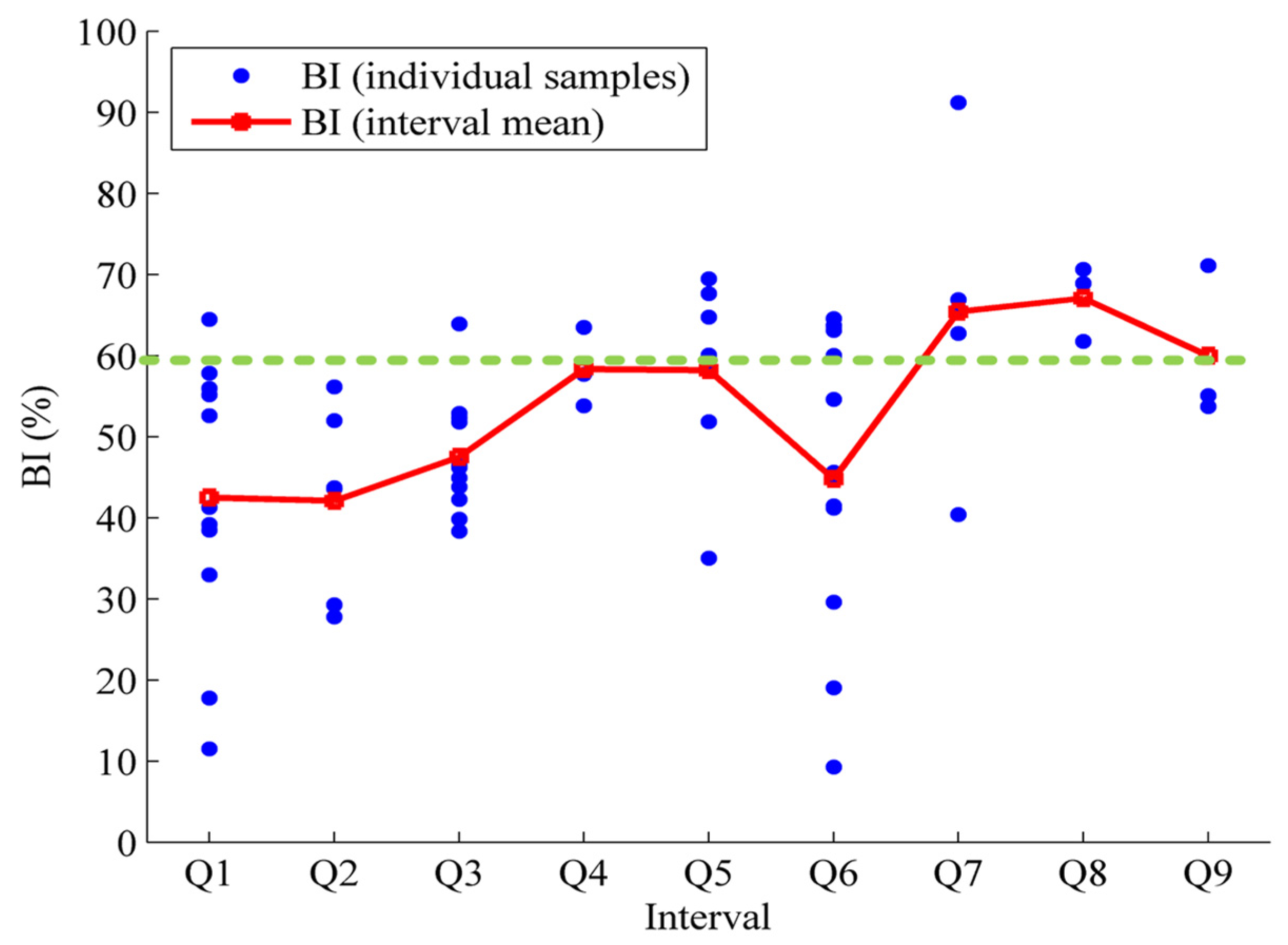
Based on the interval-scale BI comparison for the Gulong Shale (Q1–Q9), the results show that the BI values of Q1, Q2, Q3, and Q6 are clearly lower than 60%, indicating relatively low brittleness and a stronger tendency toward plastic/ductile deformation. In contrast, the BI values of Q4, Q5, and Q9 are close to 60%, corresponding to a moderately to relatively high brittleness level, whereas those of Q7 and Q8 exceed 60%, representing highly brittle intervals (Figure 13). This interval-scale pattern is generally consistent with the stratified results derived from the ternary indices. It should be noted, however, that BI essentially compresses E and v into a single composite measure, primarily reflecting the combined effects of stiffness and Poisson’s ratio. Therefore, BI is more suitable as an elastic-level overall reference, but it is insufficient to further discriminate whether the observed fracability differences are predominantly controlled by fracture initiation thresholds, propagation limitations, or fracture-network development modes.

Figure 13. Interval-scale distribution of BI for the Gulong Shale (Q1–Q9) and comparison with interval means (Note: the green line denotes the 60% threshold for brittleness classification).

In addition, Imaging logging data shows that the Q1–Q3 intervals have weak development and extremely poor connectivity of natural fractures and bedding fractures, with natural fractures mainly concentrated in the Q5, Q7, Q8, and Q9 oil intervals [50]; The Q1–Q9 intervals exhibit a vertical differentiation characteristic of “upper ductile and lower brittle” in mineral composition, where the Q1–Q2 intervals have higher plasticity and poor fracability, while the Q8–Q9 intervals have high brittleness and excellent fracture propagation capability, making them the optimal fracturing target layers in this region [51,52].

It is worth noting that the ternary index method adopted in this study for evaluating Gulong Shale did not take into account the anisotropy of shale, with the focus on establishing an evaluation method based on the three-level framework of fracture “initiation–propagation–network formation”. In this study, the mechanical properties of rocks perpendicular to the bedding direction were mainly considered. For the mechanical properties of shale with different bedding orientations, this method can also be applied for evaluation based on measured data. Beyond anisotropy, the framework also has several boundaries of applicability that deserve discussion. Because the indices are normalized within the studied dataset, they are best understood as reflecting relative ranking in the current study area, and the classification criteria may need to be re-established when the workflow is transferred to other formations. Uncertainty can also be influenced by data coverage, especially for fracture toughness, which is typically difficult to obtain and characterized by sparse and uneven distribution across wells and intervals. Furthermore, although interval-scale averages are useful for describing stratigraphic trends, such values should only be regarded as indicative indicators in view of the objective existence of inter-well heterogeneity. The proposed framework is intentionally built around key mechanical controls along the fracture-evolution chain, while geological descriptors such as natural-fracture density, mineralogy, and bedding characteristics are not explicitly included; these factors remain important and can be incorporated as complementary constraints in future improvements.

7. Conclusions

• A new mechanical deformation modulus for characterizing rock fracture development modes was proposed (deformation modulus $E_F=E·e^{-{\displaystyle \frac{{\sigma }_3}{{\sigma }_1-{\sigma }_3}}}=E·e^{-{\displaystyle \frac{1}{k}}}$), based on the control mechanism of stress conditions and Young’s modulus on fracture modes. Three distinct fracture mode grades were defined: E_F < 10 GPa corresponds to deformation model I, where macroscopic rock fracturing is insignificant, fracture apertures are small, and fracture-forming capacity is weak; 10 GPa < E_F < 15 GPa represents deformation model II, characterized by dispersed strain, development of scattered fractures, and complex low-angle fracture networks; and E_F > 15 GPa indicates deformation model III, featuring concentrated strain and a tendency to form interconnected high-angle fracture networks.
• A “ternary index” evaluation method for rock mechanical deformation heterogeneity was proposed, based on tensile strength (fracture crack index, FCI), fracture toughness (fracture growth index, FGI), and mechanical deformation modulus (fracture mode index, FMI), providing a new approach for quantifying mechanical heterogeneity in shale.
• A comprehensive shale fracability evaluation model was established based on the ternary index method, classifying its mechanical properties into four models: (1) “low tensile–low toughness–low modulus” (Q2), where fractures crack and grow easily, classified as deformation model I, featuring small fracture apertures or weak fracture-forming capability; (2) “low tensile–low toughness–medium modulus” (Q1, Q3, Q6), where fractures crack and grow easily, classified as deformation model II, forming low-angle intersecting fracture networks; (3) “low tensile–low toughness–high modulus” (Q7, Q9), where fractures crack and grow easily, classified as deformation model III, creating large-aperture, high-angle through-going fracture networks; (4) and “high tensile–low toughness–high modulus” (Q4, Q5, Q8), where fractures crack with difficulty (low fracture density) but grow easily, classified as deformation model III, developing high-angle through-going shear fractures.
• The evaluation results obtained using the ternary index method show strong agreement with the actual reservoir fracability characteristics. Compared with conventional brittleness evaluation methods based on elastic parameters, both approaches yield generally consistent conclusions regarding the hydraulic-fracturing quality of each stratigraphic interval. However, conventional methods cannot effectively discriminate the fracture-development characteristics during fracturing. In contrast, the ternary index method provides a comprehensive prediction of fracture initiation potential, propagation capacity, and fracture mode, thereby offering key technical support for fracture-network forecasting and fracture-connectivity assessment in field hydraulic-fracturing operations. Overall, this method possesses both solid theoretical value and practical guidance significance, with promising prospects for broader application.

References

- Holditch, S.A. Tight Gas Sands. J. Pet. Technol. 2006, 58, 86–93. [Google Scholar] [CrossRef] [Scilit]
- Hu, W.; Bao, J.; Hu, B. Practice of Unconventional Gas Development and Engineering Management Innovation in China. Front. Eng. Manag. 2014, 1, 18–29. [Google Scholar] [CrossRef] [Scilit]
- Zou, C.N.; Zhang, G.S.; Yang, Z.; Tao, S.Z.; Hou, L.H.; Zhu, R.K.; Yuan, X.J.; Ran, Q.Q.; Li, D.H.; Wang, Z.P. Concept, characteristics, potential and technology of unconventional oil and gas: Also on unconventional petroleum geology. Pet. Explor. Dev. 2013, 40, 385–399+454. [Google Scholar] [CrossRef] [Scilit]
- Pollastro, M.R. Total petroleum system assessment of undiscovered resources in the giant Barnett Shale continuous (unconventional) gas accumulation, Fort Worth Basin, Texas. AAPG Bull. 2007, 91, 551–578. [Google Scholar] [CrossRef] [Scilit]
- Cao, D.Y.; Yao, Z.; Li, J. Research status and development trend of unconventional natural gas evaluation in coal measures. Coal Sci. Technol. 2014, 42, 89–92+105. [Google Scholar] [CrossRef]
- Li, X.J.; Hu, S.Y.; Cheng, K.M. Suggestions from the development of fractured shale gas in North America. Pet. Explor. Dev. 2007, 34, 392–400. [Google Scholar] [CrossRef]
- Yang, Z.; Zou, C.N. “Exploring petroleum inside source kitchen”: Connotation and prospect of source rock oil and gas. Pet. Explor. Dev. 2019, 46, 12. [Google Scholar] [CrossRef] [Scilit]
- Guo, X.; Wang, R.; Shen, B.; Wang, G.; Wan, C.; Wang, Q. Geological characteristics, resource potential, and development direction of shale gas in China. Pet. Explor. Dev. Online 2025, 52, 17–32. [Google Scholar] [CrossRef] [Scilit]
- He, Z.L.; Nie, H.K.; Jiang, T.X. Challenges and countermeasures for large-scale and effective development of deep shale gas in the Sichuan Basin. Reserv. Eval. Dev. 2021, 11, 1–11+41. [Google Scholar] [CrossRef]
- Zhang, B.W.; Zhang, J.H.; Feng, Z.H.; Zeng, H.S.; Huo, Q.L.; Zhang, K. Geological conditions and resource potential for the formation of light crude oil from Gulong shale in Q ingshankou Formation, Songliao Basin. Acta Pet. Sin. 2021, 42, 1625–1639. [Google Scholar] [CrossRef]
- Yang, Z.; Zou, C.N.; Fu, J.H.; Wu, S.T.; Lin, S.H.; Pan, S.Q.; Wang, L.; Liu, X.S.; Niu, X.B. Characteristics and “Sweet Area(Section)” Evaluation of Continuous Tight & Shale Oil and Gas in Ordos Basin, North-central China. J. Earth Sci. Environ. 2019, 41, 459–474. [Google Scholar] [CrossRef]
- Goodarzi, M.; Rouainia, M.; Aplin, A.; Cubillas, P.; de Block, M. Predicting the elastic response of organic-rich shale using nanoscale measurements and homogenisation methods. Geophys. Prospect. 2017, 65, 1597–1614. [Google Scholar] [CrossRef] [Scilit]
- Zou, C.; Zhu, R.; Wu, S.; Yang, Z.; Tao, S.; Yuan, X. Types, characteristics, mechanisms and prospects of conventional and unconventional oil and gas accumulation: A case study of tight oil and tight gas in China. Acta Pet. Sin. 2012, 33, 173–187. [Google Scholar] [CrossRef]
- Zhong, Y.; Yu, H.; Wang, Q.; Chen, X.; Ke, X.; Huang, H.; Wu, H. Hydraulic fracturing in layered heterogeneous shale: The interaction between adjacent weak interfaces. Eng. Fract. Mech. 2024, 303, 110115. [Google Scholar] [CrossRef] [Scilit]
- Fu, H.F.; Cai, B.; Geng, M.; Jia, A.L.; Weng, D.W.; Liang, T.C.; Zhang, F.S.; Wen, X.Y.; Xiu, N.L. Three dimensional simulation of hydraulic fracture propagation based on vertical reservoir heterogeneity. Nat. Gas Ind. 2022, 42, 56–68. [Google Scholar] [CrossRef]
- Zhao, J.Z.; Ren, L.; Hu, Y.Q. Controlling factors of network fracturing in shale reservoirs. J. Southwest Pet. Univ. (Sci. Technol. Ed.) 2013, 35, 1–9. [Google Scholar] [CrossRef]
- Rysak, B.; Gale, J.F.; Laubach, S.E.; Ferrill, D.A. Mechanisms for the Generation of Complex Fracture Networks: Observations From Slant Core, Analog Models, and Outcrop. Front. Earth Sci. 2022, 10, 848012. [Google Scholar] [CrossRef] [Scilit]
- Hou, Z.-K.; Cheng, H.-L.; Sun, S.-W.; Chen, J.; Qi, D.-Q.; Liu, Z.-B. Crack propagation and hydraulic fracturing in different lithologies. Appl. Geophys. 2019, 16, 243–251. [Google Scholar] [CrossRef] [Scilit]
- Li, W.; Li, Z.; Li, Y.; Zhao, H.; Wang, S.; Xu, X.; Kong, J. Study on the extension law of fractures in shale reservoirs under impact loads. PLoS ONE 2025, 20, e0328782. [Google Scholar] [CrossRef] [Scilit]
- Roylance, D. Introduction to Fracture Mechanics; Massachusetts Institute of Technology, Department of Materials Science and Engineering: Cambridge, MA, USA, 2001. [Google Scholar]
- Sun, J.M.; Han, Z.L.; Qin, R.B.; Zhang, J. Logging evaluation method for fracability of tight gas reservoirs. Acta Pet. Sin. 2015, 36, 74–80. [Google Scholar] [CrossRef]
- Zeng, Z.P.; Liu, Z.; Ma, J.; Zhang, C.L.; Li, J.; Liu, Z.; Sun, L.N. A new method for fracability evaluation of deep tight sandstone reservoirs. J. Geomech. 2019, 25, 223–232. [Google Scholar] [CrossRef]
- Hiyama, M.; Shimizu, H.; Ito, T.; Tamagawa, T.; Tezuka, K. Distinct Element Analysis for hydraulic fracturing in shale-effect of brittleness on the fracture propagation. In Proceedings of the 47th US Rock Mechanics/Geomechanics Symposium, San Francisco, CA, USA, 23–26 June 2013; American Rock Mechanics Association: Westminster, CO, USA, 2013. [Google Scholar]
- Wang, S. Main Controlling Factors of Brittleness and Fracability Classification Evaluation for Tight Reservoirs. Ph.D. Thesis, Northeast Petroleum University, Daqing, China, 2022. [Google Scholar] [CrossRef]
- Jin, X.; Shah, S.N.; Roegiers, J.-C.; Zhang, B. Fracability evaluation in shale reservoirs—An integrated petrophysics and geomechanics approach. In Proceedings of the SPE Hydraulic Fracturing Technology Conference, The Woodlands, TX, USA, 4–6 February 2014. Paper No. SPE-168589-MS. [Google Scholar]
- Yuan, J.; Zhou, J.; Liu, S.; Feng, Y.; Deng, J.; Xie, Q.; Lu, Z. An improved fracability-evaluation method for shale reservoirs based on new fracture toughness-prediction models. SPE J. 2017, 22, 1704–1713. [Google Scholar] [CrossRef] [Scilit]
- Andreev, G.E. Brittle Failure of Rock Materials: Test Results and Constitutive Models; A. A. Balkema: Rotterdam, The Netherlands, 1995; pp. 123–128. [Google Scholar]
- Hucka, V.; Das, B. Brittleness determination of rocks by different methods. Int. J. Rock Mech. Min. Sci. 1974, 11, 389–392. [Google Scholar] [CrossRef] [Scilit]
- Antonellini, M.A.; Aydin, A.; Pollard, D.D. Microstructure of deformation bands in porous sandstones at Arches National Park, Utah. J. Struct. Geol. 1994, 16, 941–959. [Google Scholar] [CrossRef] [Scilit]
- Hajiabdolmajid, V.; Kaiser, P. Brittleness of rock and stability assessment in hard rock tunneling. Tunn. Undergr. Space Technol. 2003, 18, 35–48. [Google Scholar] [CrossRef] [Scilit]
- Honda, H.; Sanada, Y. Hardness of coal. Fuel 1956, 35, 451–461. [Google Scholar]
- Lawn, B.R.; Marshall, D.B. Hardness, toughness, and brittleness: An indentation analysis. J. Am. Ceram. Soc. 1979, 62, 347–350. [Google Scholar] [CrossRef] [Scilit]
- Bažant, Z.P.; Kazemi, M.T. Determination of fracture energy, process zone length and brittleness number from size effect, with application to rock and concrete. Int. J. Fract. 1990, 44, 111–131. [Google Scholar] [CrossRef] [Scilit]
- Quinn, J.B.; Quinn, G.D. Indentation brittleness of ceramics: A fresh approach. J. Mater. Sci. 1997, 32, 4331–4346. [Google Scholar] [CrossRef] [Scilit]
- Yagiz, S. An investigation on the relationship between rock strength and brittleness. In Proceedings of the 59th Geological Congress of Turkey, Ankara, Turkey, 20–24 March 2006; p. 352. [Google Scholar]
- Copur, H.; Bilgin, N.; Tuncdemir, H.; Balci, C. A set of indices based on indentation test for assessment of rock cutting performance and rock properties. J. South. Afr. Inst. Min. Metall. 2003, 103, 589–600. [Google Scholar]
- Rickman, R.; Mullen, M.; Petre, E.; Grieser, B.; Kundert, D. A practical use of shale petrophysics for stimulation design optimization: All shale plays are not clones of the Barnett shale. In Proceedings of the SPE Annual Technical Conference and Exhibition, Denver, CO, USA, 21–24 September 2008. SPE-115258-MS. [Google Scholar]
- Feng, T.; Xie, X.B. Brittleness of rocks and brittleness indexes for describing rockburst proneness. Min. Metall. Eng. 2000, 20, 18–20. [Google Scholar]
- Protodyakonov, M.M. Mechanical properties and drillability of rocks. In Proceedings of the 5th Symposium on Rock Mechanics, Minneapolis, MN, USA, May 1963; University of Minnesota Press: Minneapolis, MN, USA, 1963; pp. 103–118. [Google Scholar]
- Bishop, A.W. Progressive failure with special reference to the mechanism causing it. In Proceedings of the Geotechnical Conference on the Shear Strength Properties of Natural Soils and Rocks, Oslo, Norway, 19–22 September 1967; pp. 142–150. [Google Scholar]
- Altindag, R. Correlation of specific energy with rock brittleness concept on rock cutting. J. South. Afr. Inst. Min. Metall. 2003, 103, 163–171. [Google Scholar]
- Tarasov, B.; Potvin, Y. Universal criteria for rock brittleness estimation under triaxial compression. Int. J. Rock Mech. Min. Sci. 2013, 59, 57–69. [Google Scholar] [CrossRef] [Scilit]
- Wang, S.; Xu, K.; Zhao, W.; Fu, X.; Lu, X.; Song, Z. A New Model to Predict Mudstone Failure Behavior from Brittle to Ductile Caused by Confining Pressures. Processes 2025, 13, 308. [Google Scholar] [CrossRef] [Scilit]
- Byerlee, J.D. Friction of rocks. Pure Appl. Geophys. 1978, 116, 615–626. [Google Scholar] [CrossRef] [Scilit]
- Meglis, I.L.; Greenfield, R.J.; Engelder, T.; Graham, E.K. Pressure dependence of velocity and attenuation and its relationship to crack closure in crystalline rocks. J. Geophys. Res. Solid Earth 1996, 101, 17523–17533. [Google Scholar] [CrossRef] [Scilit]
- Ma, Y.; Yu, C.; Li, H.B.; Cheng, Z.; Liu, Y.Q.; Wu, J.J. Coupling effects of confining pressure and strain rate on rock compressive strength. J. Rock Mech. Geotech. Eng. 2025, 17, 6881–6899. [Google Scholar] [CrossRef] [Scilit]
- ISRM Testing Commission. Suggested method for determining mode I fracture toughness using cracked chevron notched Brazilian disc (CCNBD) specimens. Int. J. Rock Mech. Min. Sci. Geomech. Abstr. 1995, 32, 57–64. [Google Scholar] [CrossRef] [Scilit]
- Wang, Q.Z.; Fan, H.; Gou, X.P.; Zhang, S. Recalibration and Clarification of the Formula Applied to the ISRM-Suggested CCNBD Specimens for Testing Rock Fracture Toughness. Rock Mech. Rock Eng. 2013, 46, 303–313. [Google Scholar] [CrossRef] [Scilit]
- Feng, C.; Liu, X. Mechanics Characteristics of Rocks in the Deep Tight Carbonate Reservoir. Int. J. Multiphysics 2021, 15, 349–362. [Google Scholar] [CrossRef] [Scilit]
- Wang, T.; Zhao, H.B.; Yang, Z.H.; Zhang, S.R.; Ren, C.F.; Tang, X.H. Influence of natural fractures in shale reservoirs on hydraulic fracturing stimulation effect: A case study of Qingshankou Formation shale in Gulong Sag, Songliao Basin. Oil Geophys. Prospect. 2025, 60, 213–224. [Google Scholar] [CrossRef]
- Sun, L.; Zhu, R.; Zhang, T.; Cai, Y.; Feng, Z.; Bai, B.; Jiang, H.; Wang, B. Advances and trends of non-marine shale sedimentology: A case study from Gulong Shale of Daqing Oilfield, Songliao Basin, NE China. Pet. Explor. Dev. 2024, 51, 1183–1198. [Google Scholar] [CrossRef] [Scilit]
- Sun, L.; Cui, B.; Zhu, R.; Wang, R.; Feng, Z.; Li, B.; Zhang, J.; Gao, B.; Wang, Q.; Zeng, H.; et al. Shale oil enrichment evaluation and production law in Gulong Sag, Songliao Basin, NE China. Pet. Explor. Dev. 2023, 50, 441–454. [Google Scholar] [CrossRef] [Scilit]
Disclaimer/Publisher’s Note: The statements, opinions and data contained in all publications are solely those of the individual author(s) and contributor(s) and not of MDPI and/or the editor(s). MDPI and/or the editor(s) disclaim responsibility for any injury to people or property resulting from any ideas, methods, instructions or products referred to in the content. |
© 2026 by the authors. Licensee MDPI, Basel, Switzerland. This article is an open access article distributed under the terms and conditions of the Creative Commons Attribution (CC BY) license.