Game Theory and Optimal Planning Strategy for Electricity Heat Multiple Heterogeneous Energy Systems Based on Deep Temporal Clustering Method

Abstract

With the continuous increase in the penetration rate of renewable energy sources, the uncertainty of new energy output has brought significant risks and challenges to the planning strategy of integrated energy systems. Meanwhile, power grid operators and heat network operators, belonging to different stakeholder entities, exhibit complex cooperative-competitive game relationships, making it difficult to balance the interests of all parties. To address this issue, this paper proposes a game theory and optimal planning strategy for electricity-heat multiple heterogeneous energy systems based on a deep temporal clustering method from the perspective of different stakeholders. Firstly, typical scenarios of renewable energy output are generated through the deep temporal clustering method. Simultaneously, the charging and discharging behaviors of energy storage devices are utilized to assist the distribution system in new energy consumption. This paper incorporates battery life degradation costs into the objective function on the power grid side to achieve accurate accounting of energy storage device dispatch expenses. Additionally, an optimal dispatch model is established on the heat network side, upon which a game framework for multiple heterogeneous energy systems is constructed. The construction capacity and installation location of each flexible device can be determined through planning decisions in typical multi-scenario situations. Considering the non-convex and nonlinear characteristics of the model, this paper employs an improved firefly algorithm to achieve optimal solution search and rapid convergence. Finally, the effectiveness and feasibility of the proposed method are demonstrated through a case study of an electricity-heat energy system.

1. Introduction

With energy and environmental issues becoming increasingly prominent, there has been a consensus on gradually transforming the energy structure and developing renewable energy sources. However, renewable energy sources such as solar and wind energy exhibit characteristics of randomness and intermittency. After their large-scale integration into the power grid, they pose significant challenges to the operation and dispatch of the power system [1]. The emergence of integrated energy systems provides an effective means for the comprehensive utilization of renewable energy. An integrated energy system is a complex energy supply system that integrates distributed power sources, energy storage, loads, and multi-energy flow systems [2]. Through the coordinated operation of internal source-storage-load units, it can achieve autonomous operation and friendly grid interaction, serving as an effective carrier for integrating large-scale distributed renewable energy into the power grid [3]. Formulating scientific coordinated operation strategies for integrated energy systems can effectively reduce operational costs and enhance the economic efficiency of energy supply [4,5].

To effectively address the severe impacts of distributed renewable energy sources on the power grid, extensive research has been conducted both domestically and internationally: Literature [6] established an optimized scheduling model for home energy management with the objectives of minimizing household electricity costs and optimizing the flatness of the net load curve, employing a binary particle swarm optimization algorithm to solve the model. Literature [7] investigated the principles and control strategies for real-time energy scheduling in microgrids, developing a microgrid energy model based on genetic algorithms; however, it did not consider the establishment of mathematical models when significant deviations exist between the power grid’s demand and scheduling requirements. Literature [8] constructed a photovoltaic (PV), diesel, and energy storage microgrid model based on time-of-use electricity pricing, designing penalty functions for energy storage charging/discharging during different periods, achieving certain results; however, it did not account for the impact of wind turbine generation on the power grid. Currently, deploying energy storage systems with a certain capacity to mitigate renewable energy fluctuations has become a crucial approach for enhancing power quality and grid operational reliability. Especially in recent years, with the rapid development of energy storage technologies and improvements in their technical performance and economic viability [9], the integration of various types of energy storage not only enhances flexibility but also reduces economic costs [10]. Literature [11] proposed a game theory-based energy storage demand response model, studying energy-sharing schemes between energy storage and community PV systems, thereby improving system economic efficiency and PV consumption. Literature [12] introduced a robust optimization-based optimal configuration scheme for energy storage systems (ESSs) to alleviate power and voltage fluctuations caused by high penetration of renewable energy sources. Currently, the primary factors hindering the widespread adoption of electrochemical energy storage are its relatively short lifespan and high costs [13]. Literature [14] considered the uncertainty of distributed generation (DG) output, employed Kantorovich distance for scenario reduction, and established a multi-objective coordinated optimization scheduling model for DG and distributed energy storage (DES) based on demand response. Literature [15] developed a frequency regulation and peak-shaving model for energy storage (ES), considering the simultaneous provision of frequency regulation and peak-shaving services by ES, and proposed a joint optimization framework. Literature [16] utilized an improved K-means++ algorithm for distributed PV (DPV) scenario reduction, considering ES peak-shaving costs, and established a multi-scenario peak-shaving model for distributed PV and energy storage. Due to constraints such as power flow, coordinated optimization scheduling models typically exhibit non-convex and nonlinear characteristics, making it difficult to obtain optimal solutions using particle swarm optimization algorithms, grey wolf optimization algorithms, etc., and resulting in long solution times [17]. This can lead to inefficient utilization of overall grid resources and certain limitations. Therefore, Ref. [18] introduced second-order cone relaxation and semidefinite relaxation to handle power flow constraints. Literature [19], in response to the uncertainty of DG output, proposed a robust planning model that comprehensively considers network loss costs and ES investment costs, transforming the original bi-level programming model into a single-level programming problem with bilinear terms through Lagrangian duality applied to a convex cone model. Literature [20] fully considered optimization objectives such as transmission network expansion and equipment siting and sizing, establishing a multi-variable coordinated planning model based on second-order cone programming (SOCP), which was solved using an improved Benders decomposition method. Literature [21] developed an economic dispatch model for DG and ES in transmission networks based on SOCP, comparing the proposed method with non-convex models and semidefinite programming to verify its accuracy.

On the other hand, to enhance the robustness of scheduling decisions, numerous scholars have employed uncertainty programming methods for modeling, transforming uncertainty optimization problems into deterministic optimization problems to simplify the solution process. Uncertainty programming methods include stochastic programming, robust optimization, and scenario analysis [22]. Stochastic programming is a traditional optimization method for addressing modeling uncertainties, often utilizing the Beta probability distribution function to establish the probability density function of photovoltaic (PV) systems [23]. Stochastic programming is only applicable when uncertainties can be accurately described by probability density functions, requiring a substantial amount of historical data for uncertainty estimation. Therefore, it is suitable for scenarios with relatively low uncertainties that necessitate precise estimation. Robust optimization is a method for solving optimization problems with parameter uncertainties, requiring only the fluctuation range of uncertain parameters rather than scenarios or precise probability distributions [24]. Due to the need to consider the worst-case scenario, which results in high computational complexity, robust optimization is suitable for scenarios with stringent requirements for modeling stability and security. Reference [25] established a robust optimization configuration model for selecting the connection points and capacities of distributed PV power plants integrated into transmission networks, calculating the probability distributions of maximum and minimum expectations in fuzzy sets through optimization. Reference [26], based on a time-series modeling approach, classified five weather types and derived probability density functions and typical daily PV output profiles by fitting distribution parameters. Scenario analysis transforms probability distribution models containing random variables into specific scenarios, simulating the distribution of the original random variables with as few scenarios as possible, thereby converting stochastic optimization problems into deterministic optimization problems [27]. This method offers strong applicability in modeling results but may lead to incomplete models due to insufficient scenario modeling. Although numerous scholars have conducted relevant research, there are still the following issues that need to be addressed:

(1)

Inadequate consideration of uncertainties in renewable energy output and complex cooperative-competitive relationships: When studying integrated energy systems, most existing literature does not fully account for the significant uncertainties in renewable energy output and the challenges they pose to system operation and planning. Simultaneously, there is a lack of in-depth analysis and modeling of the complex cooperative-competitive relationships between power grid and heat network operators, making it difficult to balance the interests of all parties.

(2)

Limitations and efficiency issues of optimization algorithms in handling non-convex and nonlinear models: When addressing optimization problems in integrated energy systems, existing methods often face challenges due to the non-convex and nonlinear nature of the models, resulting in difficulties in obtaining globally optimal solutions and long computation times. Although some literature has adopted algorithms such as PSO, limitations still exist when dealing with complex models, such as slow convergence rates and susceptibility to local optimal.

The main innovations of this paper can be summarized as follows:

(1)

Proposing a typical scenario generation method based on deep temporal clustering: This method effectively captures the complex patterns and dynamic variations in renewable energy output through deep learning models, generating more realistic typical scenarios. This approach not only improves the accuracy of scenario generation but also enhances the adaptability of scheduling plans to new energy output, contributing to a reduction in the total system operating costs.

(2)

Constructing a game theory-based optimal planning strategy for multiple heterogeneous energy systems: In response to the complex cooperative-competitive relationships between power grid and heat network operators, this paper constructs an optimal planning strategy for multiple heterogeneous energy systems based on game theory. By introducing an IFA, it effectively addresses non-convex and nonlinear optimization problems, achieving rapid convergence and a search for globally optimal solutions. This strategy not only balances the economic interests of all parties but also improves the overall planning and operational efficiency of the system, providing a new solution for addressing uncertainties in renewable energy.

2. Typical Scenario Generation Method Based on Deep Temporal Clustering

To achieve effective clustering of complex temporal sequence scenarios, based on existing research, this chapter designs a Temporal Autoencoder (TAE) structure suitable for feature extraction from multidimensional temporal data. It proposes a Deep Temporal Clustering (DTC) algorithm that jointly optimizes temporal feature extraction and temporal clustering, along with evaluation metrics for assessing the clustering performance of temporal data.

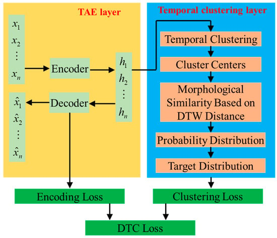
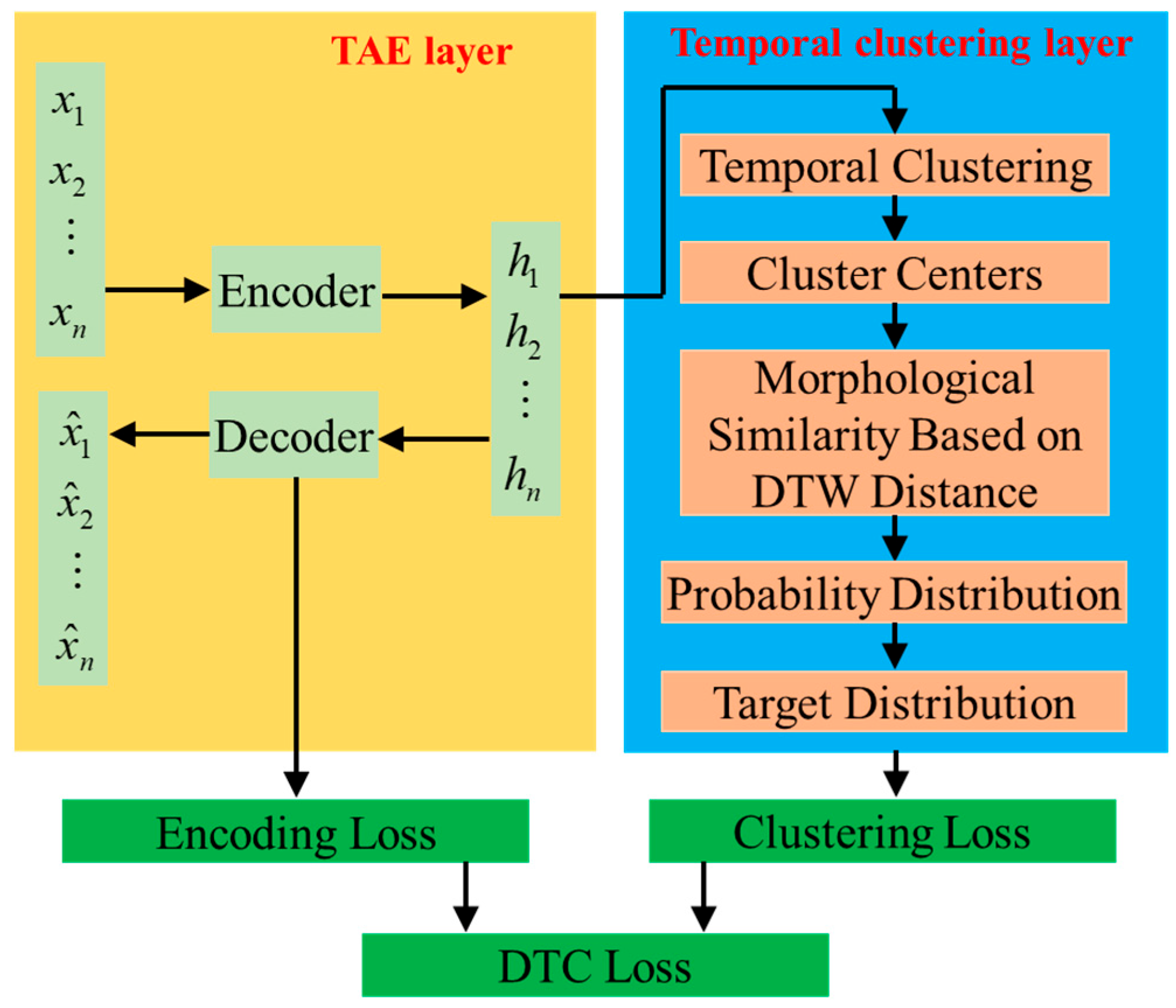
The specific details of the algorithm are as follows: Consider n multidimensional time series x₁, x₂, …, x_n, where each time series has f-dimensional features and a temporal length of T, i.e., x_i ∈ ℝ^f×T, i ∈ [1, n]. The objective of the DTC algorithm is to classify these n multidimensional time series into k clusters, where 1 ≤ k ≤ n, based on the deep-level features h_i of the multidimensional time series x_i and the morphological similarity between time series. The DTC algorithm primarily consists of two parts: the TAE and temporal clustering. The TAE model performs deep-level feature extraction and data dimensionality reduction for multidimensional time series, while the temporal clustering layer calculates morphological similarity based on the deep-level features using Dynamic Time Warping (DTW) distance, achieving temporal clustering and identifying cluster centers. The main framework of the DTC algorithm is illustrated in Figure 1. This paper employs the DTC method to synchronize the response times of power grids and heat networks: Firstly, the original multiscale time series data is normalized and resampled to the hourly level to establish a unified time baseline; Secondly, a time series autoencoder is utilized to hierarchically extract multidimensional features, avoiding interference and achieving effective coupling; Finally, time series shape similarity clustering is conducted based on DTW, ignoring differences in absolute response times and focusing on relative change patterns. Through these three steps, effective fusion and synchronous clustering of time series data from energy subsystems with different response time scales are achieved.

Figure 1. Framework of the DTC algorithm.

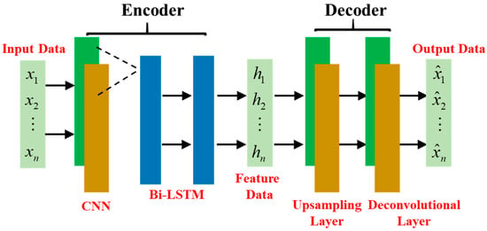
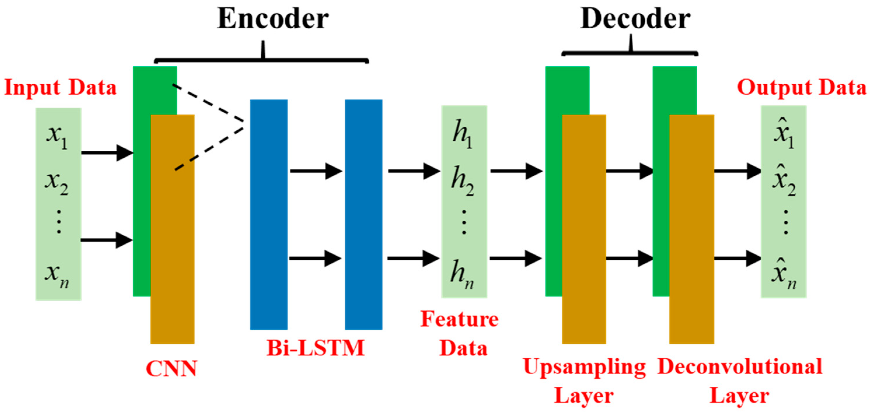
In unsupervised learning, the autoencoder (AE) is a neural network model commonly used for deep-level feature extraction and data dimensionality reduction, finding wide applications in areas such as image and text feature extraction. An AE primarily consists of two parts: an encoder and a decoder. Its core principle lies in leveraging the nonlinear mapping capabilities of neural networks to extract deep-level features from raw data in the encoder, mapping the original data to a low-dimensional space with minimal feature loss. Subsequently, in the decoder, the low-dimensional deep-level features are inversely mapped and reconstructed back into the original data. To fully extract deep-level features from multidimensional time series, the structure of the Temporal Autoencoder (TAE) designed in this paper is illustrated in Figure 2.

Figure 2. The structure of the TAE.

The loss function of the TAE is the mean square error (MSE) between the reconstructed output data from the decoder and the original data input to the encoder, expressed as:

$$L_{rec}={\displaystyle \frac{1}{n}}{\displaystyle \sum _{i=1}^n{‖x_i-{\widehat{x}}_i‖}^2}$$

(1)

Based on the deep-level features of the original data extracted by the TAE model, the temporal clustering layer calculates the morphological similarity between time series using the DTW distance, partitions the original data into clusters, and identifies the cluster centers. The core parameters of the temporal clustering layer are the k cluster centers, denoted as c_i ∈ ℝ^1×H, where i ∈ [1, k]. Leveraging the deep-level features h_i of the original data obtained from the TAE, the temporal clustering layer computes the morphological similarity between h_i and each cluster center c_j based on the DTW distance. It then normalizes the DTW distances using a t-distribution with one degree of freedom to perform probabilistic soft assignment of the data points to the clusters.

$$q_{ij}={\displaystyle \frac{{[1+D_{dtw}(h_i,c_j)]}^{-1}}{{\displaystyle \sum _{j=1}^k{[1+D_{dtw}(h_i,c_j)]}^{-1}}}}$$

(2)

Here, q_ij represents the probability that the encoded data h_i belongs to the cluster center c_j. The clustering problem in this paper falls under unsupervised learning, where true cluster labels are unavailable. Therefore, a target distribution p is employed to approximate the true distribution, with its elements p_ij defined as shown in Equation (3). This approach effectively enhances high-confidence predictions and normalizes the loss, thereby preventing potential representation distortion.

$$p_{ij}={\displaystyle \frac{q_{ij}^2/{\displaystyle \sum _{i=1}^n{q}_{ij}}}{{\displaystyle \sum _{j=1}^k(q_{ij}^2/{\displaystyle \sum _{i=1}^n{q}_{ij}})}}}$$

(3)

The loss function of the temporal clustering layer is the Kullback–Leibler (KL) divergence value between the probability distribution q and the target distribution p, which can be calculated according to (4).

$$L_c{\displaystyle \sum _{i=1}^n{\displaystyle \sum _{j=1}^k{p}_{ij}{\log }_2\frac{p_{ij}}{q_{ij}}}}$$

(4)

The loss function L of the DTC algorithm is composed of the encoding-reconstruction loss L_rec and the clustering loss L_c, as shown in Equation (5). Here, λ is a settable weight parameter. To prevent excessive distortion of the encoding space of the TAE model during the training of the temporal clustering layer, λ is typically set to 0.9. The weight factor λ in Formula (5) is set to 0.9, which is optimized and selected through grid search experiments in combination with indicators such as the TSC, rather than being a mere empirical value. Experiments show that the clustering effect is poor when λ < 0.8; when λ ∈ [0.8, 0.95], the TSC value (0.92) and typical scenario coverage (96.7%) are both optimal at λ = 0.9; when λ > 0.95, clustering loses a reliable feature basis. Therefore, λ = 0.9 represents the optimal trade-off between ensuring the accuracy of temporal feature extraction and achieving effective clustering, with stable and reliable clustering results.

$$L=\lambda L_{rec}+(1-\lambda )L_c$$

(5)

This paper employs Dynamic Time Warping (DTW) morphological distance as the distance calculation method and proposes the Temporal Silhouette Coefficient (TSC) metric to evaluate the effectiveness of clustering for time-series data:

$$TSC={\displaystyle \frac{b_i-a_i}{\max (a_i,b_i)}}$$

(6)

Here, a_i represents the average DTW distance between the given sample and other samples within the same class; b_i denotes the average DTW distance between the given sample and all samples in other classes. The TSC metric can quantify the degree of temporal morphological similarity of a time-series sample to its own cluster compared to other clusters, with a value range of [−1, 1]. A higher value indicates greater temporal similarity between the sample and its own cluster, and lower temporal similarity with other clusters, suggesting better performance of the time-series clustering.

3. Battery Lifespan and Depreciation Cost Model

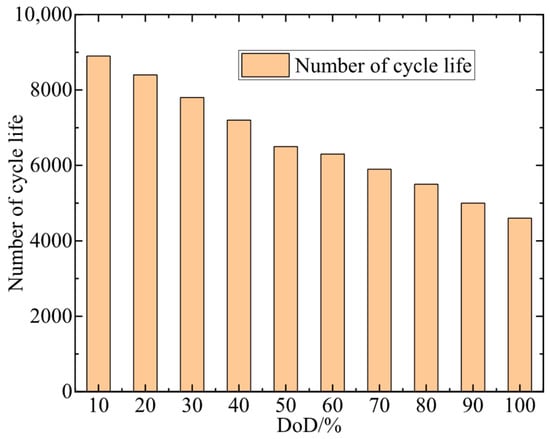
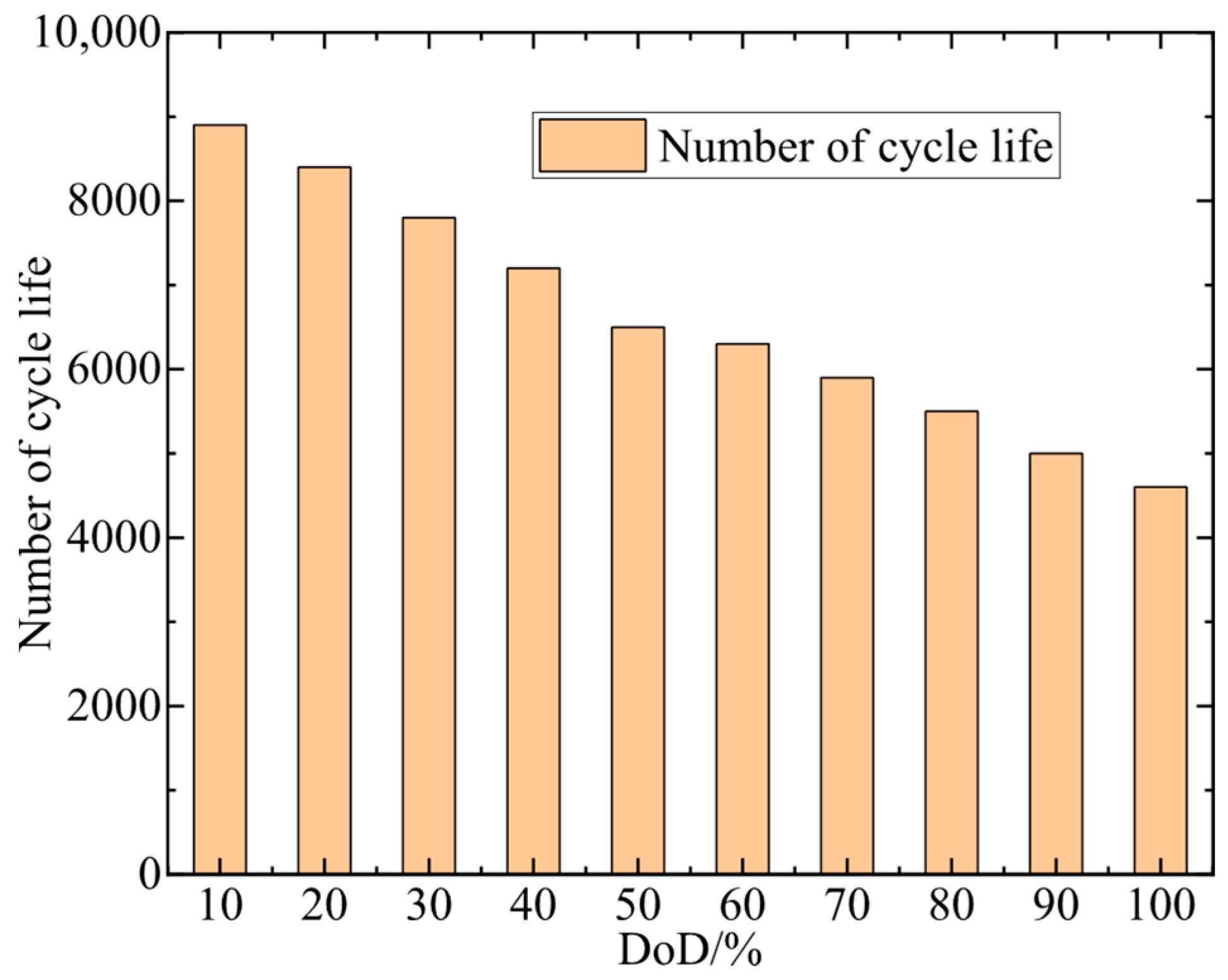
Under a low cycling frequency with daily single charge and single discharge, electrochemical energy storage systems can generally last until their expected lifespan. However, the combination of frequent charge–discharge cycles and a low state of charge will significantly shorten the battery’s expected lifespan. Therefore, it is necessary to consider short-term planning in scheduling, namely, the impact of the number of charging cycles and the depth of charge–discharge within a day on the battery’s overall lifespan. For lithium iron phosphate (LIP) batteries manufactured using different technologies, the exponential relationship between their demonstrated cycle life and depth of discharge varies. Figure 3 illustrates the cycle life of a typical LIP battery.

Figure 3. Cycle life of a typical LIP battery.

Based on Figure 3, the functional relationship between cycle life and depth of discharge (DoD) can be fitted as follows:

$$N_{cal}=4700*{(DoD)}^{-0.5}$$

(7)

Here, $N_{cal}$ represents the number of cycles a battery can undergo before reaching its end-of-life criteria; DoD refers to the depth to which a battery is discharged during its charge–discharge cycles. As seen from Equation (7), with an increase in DoD, the battery’s lifecycle decreases in a nonlinear manner. The data on the relationship between cycle life and depth of discharge (DoD) for LIP batteries in Figure 3 of this paper is obtained by integrating benchmark data from industry-wide databases with calibration data from mainstream manufacturers. The core benchmark data is sourced from electrochemical energy storage industry-wide databases, etc., which integrate publicly available test data from leading manufacturers both domestically and abroad. Public product datasheets from mainstream manufacturers such as CATL are selected for local calibration of the foundational data. The integrated data is then subjected to exponential fitting and validated against performance test data from national standards to ensure accuracy and engineering practicality.

The daily life degradation cost of a battery depends on its usage on that particular day. Therefore, by quantifying the number of battery cycles and the depth of discharge, we can estimate the operational and maintenance costs associated with the battery’s lifespan. Under ideal operating conditions, the battery can undergo a complete charge–discharge cycle during scheduling, with its conversion coefficient E_z being defined as (8).

$$E_z={\displaystyle \frac{N_0}{N_{cal}}}={\displaystyle \frac{N_0}{N_0{(DoD)}^{-a}}}={\displaystyle \frac{1}{{(DoD)}^{-a}}}$$

(8)

Here, N₀ represents the number of cycles a battery can undergo when charged and discharged at a 100% depth of discharge; a is a constant obtained through fitting.

In actual operating conditions, to maximize economic returns, the optimal scheduling result for energy storage equipment may not involve a unidirectional full charge-full discharge cycle within a working day. The cost degradation caused by irregular charging and discharging of the energy storage equipment cannot be simply derived from (8). Therefore, it is necessary to convert the number of cycles consumed at different discharge depths of the battery over various time periods into equivalent cycle numbers at a 100% DoD. The corresponding conversion coefficient, E_eq, is defined as (9).

$$E_{eq}={\displaystyle \sum _{t=1}^T(\frac{1}{{(Do{D}_t)}^{-a}}-\frac{1}{{(Do{D}_{t-1})}^{-a}})}$$

(9)

Here, ${(Do{D}_t)}^{-a}$ represents the cycle life at the discharge depth at time t; Equation (9) only considers the impact of the battery’s discharge process on its lifespan, while the charging process can be disregarded due to its relatively minor contribution to battery life degradation. Using the battery cycle conversion coefficient E_eq for a standard working day derived from Equation (9), the battery’s operational lifespan T_cal can be further calculated as shown in Equation (10). In Equation (9), the influence of charging thermal stress is not taken into account for the time being in this paper. The scheduling and operation of battery energy storage equipment adhere to a controlled C-rate charging and discharging management strategy, which strictly limits the charging and discharging power and rate within the low C-rate safe charging and discharging range specified by the battery manufacturer (typically ranging from 0.2 C to 0.5 C), excluding rapid charging scenarios encountered in practical engineering applications. Under the controlled low C-rate charging mode, the heat generation rate during the battery charging and discharging processes is low, and the accompanying heat dissipation devices of the energy storage system can promptly dissipate the small amount of heat generated, ensuring that the battery temperature remains consistently within the safe operating range.

$$T_{cal}={\displaystyle \frac{N_0}{365*E_{eq}}}$$

(10)

The operational lifespan of the battery can be determined by dividing the number of cycles at a 100% DoD by the converted number of cycles over a typical working day, and then dividing this result by the number of days in a year. Given that the normal operational lifespan of a battery can reach 10 years or more, considering the impact of inflation, it is unreasonable to directly divide the initial investment cost of the battery, C_bin, by its operational lifespan, T_cal. Therefore, a capital recovery factor is required for adjustment, and the average daily investment cost is calculated as follows:

$$C_b=[C_{bin}{\displaystyle \frac{r{(1+r)}^{T_{cal}}}{{(1+r)}^{T_{cal}}-1}}+C_{bw}{T}_{cal}]/365$$

(11)

Here, r represents the annual interest rate; C_bw denotes the annual maintenance cost of the battery.

As seen from Equations (8) to (11), except for DoD serving as a decision variable, all other parameters are either predetermined or can be derived from DoD. Therefore, Equation (11) can be subjected to piecewise linearization to expedite the solution speed of optimal scheduling. The expression for the battery’s daily investment cost after piecewise linearization is as follows:

$$C_b^f={\displaystyle \sum _{t=1}^T(K^{d}Do{D}_t^d+B^d)}$$

(12)

Here, $Do{D}_t^d$ represents the change in the battery’s DoD during time period t; $K^d$ and $B^d$ are parameters obtained through piecewise linearization at different DoDs according to Equation (11).

4. Optimal Planning Strategy for Electricity-Heat Multiple Heterogeneous Energy Systems

4.1. Planning Strategy for Electricity Energy Systems

The optimization objective of power grid planning is to balance the economic benefit function and the State of Charge (SOC) health function of energy storage devices. Among these, economic benefit serves as the primary indicator for scheduling optimization, with the life degradation cost of energy storage devices incorporated into the economic benefit objective by converting it into economic terms. The SOC health function, acting as a secondary indicator, aims to delay the life attenuation of energy storage devices. Based on this, the objective function for power grid planning is formulated as follows:

$$\min (F)=\min (C_1+\lambda F_2)$$

(13)

Here, C₁ represents the system’s economic benefit function; F₂ is the SOC health assessment function; λ is the weighting coefficient for function F₂. The ratio of the function value of C₁ to that of λF₂ is set within a reasonable range to ensure the economic efficiency of the optimization model.

Economic benefit is an important metric for evaluating the operation of power grid equipment, with the function specifically encompassing electricity purchase and sale costs C_e, costs associated with the use of new energy sources C_r, and expenses related to the life degradation of energy storage devices C_b. Its expression is as follows:

$$C_1=C_e+C_r+C_b$$

(14)

The electricity charge depends on the power delivered by the feeder into the park area. When the microgrid experiences a power shortage, it can purchase electricity from the upper-level grid through interconnection lines. Conversely, when there is an excess of local electricity, it can sell the surplus back to the upper-level grid to generate revenue. Therefore, this portion of the cost can be calculated according to the following (15):

$$C_e={\displaystyle \sum _{t=1}^T({\lambda }_{buy}{P}_t^{buy}-}{\lambda }_{sell}{P}_t^{sell})$$

(15)

The cost of using new energy sources includes the cost of power generation from new energy and the penalty cost for wind/solar curtailment, as shown in the following Equation (16):

$$C_r={\displaystyle \sum _{t=1}^T\left[({\lambda }_{new}{P}_t^{new}+{\lambda }_{pen}(P_{total,t}^{new}-P_t^{new})\right]}$$

(16)

The daily degradation cost of energy storage, C_b, has already been provided in Equation (11) and will not be elaborated on further here. Among them, the initial investment cost, C_bin, and the maintenance cost, C_bw, are respectively as follows:

$$\left\{\begin{array}{c}{C}_{bin}={\displaystyle \sum _{n=1}^N(C_p{P}_n+C_E{E}_n)}\\ C_{bw}={\displaystyle \sum _{n=1}^N(C_w{P}_n)}\end{array}\right.$$

(17)

Here, n represents the number of individual energy storage devices; N is the total number of energy storage devices; $C_p$ denotes the cost per unit of charging/discharging power for the energy storage devices; $P_n$ is the rated charging/discharging power of the nth energy storage device; $C_E$ signifies the cost per unit of capacity for the energy storage devices; $E_n$ is the rated capacity of the nth energy storage device; $C_w$ is the annual maintenance cost per unit of charging/discharging power for the energy storage devices. Equation (18) reflects the operating conditions of each energy storage device within the system, enabling coordinated operation among the devices during scheduling and enhancing the flexibility of energy storage device dispatching.

When modeling each device in the energy storage system independently, setting up an SOC health assessment function can extend the lifespan of the energy storage devices by optimizing and coordinating the power output tasks among the devices and the power output commands for individual devices. The assessment function specifically includes an output coordination index among chemical energy storage devices $F_{ave}$, and an index to prevent frequent charging and discharging of the energy storage devices. Its expression is as follows:

$$F_{ave}={\displaystyle \sum _{t=1}^T{\displaystyle \sum _{n=1}^N\left|SO{C}_t^{ave}-SO{C}_t\right|}}$$

(18)

Here, $SO{C}_t^{ave}$ represents the average SOC of all energy storage devices during time period t; $SO{C}_t$ denotes the SOC of the n-th energy storage device during time period t.

Frequent charging and discharging of energy storage devices can also adversely affect their lifespan. Therefore, a fluctuation penalty function is established to suppress frequent SOC fluctuations in each energy storage device. Its expression is as follows:

$$F_{wav}={\displaystyle \sum _{t=1}^T{\displaystyle \sum _{n=1}^N\left|SO{C}_{total}^{ave}-SO{C}_t\right|}}$$

(19)

Here, $SO{C}_{total}^{ave}$ represents the average SOC of all energy storage devices over the entire time period.

During operation, the power grid side also needs to meet certain safety and operational state constraints, as shown below:

(1)

Power balance constraint

$$P_t^{new}+P_t^G+P_t^{buy}+P_t^{dis}=P_t^{sell}+P_t^{cha}$$

(20)

Here, $P_t^G$ represents the unit power output in the power grid at time t; $P_t^{buy}$ and $P_t^{sell}$ respectively represent the electricity purchase quantity and sales quantity from the microgrid to the upper-level grid at time t. $P_t^{dis}$ and $P_t^{cha}$ represent the discharging and charging power of the pure energy storage device at time t.

(2)

Tie-line power constraints

$$\begin{array}{l}0\le P_t^{buy}\le P_{\max }^{tie}\\ 0\le P_t^{sell}\le P_{\max }^{tie}\\ P_t^{buy}{P}_t^{sell}=0\end{array}$$

(21)

Here, $P_{\max }^{tie}$ represents the maximum transmission power of the tie-line.

(3)

Energy storage operation constraints

$$0\le P_t^{dis}\le u_t^{dis}{P}_{\max }^{dis}$$

(22)

$$0\le P_t^{cha}\le u_t^{cha}{P}_{\max }^{cha}$$

(23)

$$0\le u_t^{dis}+u_t^{cha}\le 1$$

(24)

Here, $u_t^{dis}$ and $u_t^{cha}$ are 0–1 variables, representing the discharging and charging states of energy storage, respectively. It should be noted that at the same time instant, energy storage can only operate in one of the charging or discharging states.

(4)

Renewable energy output constraints

$$0\le P_t^G\le P_{\max }^G$$

(25)

$$\Delta P_{\min }^G\le P_t^G-P_{t-1}^G\le \Delta P_{\max }^G$$

(26)

Here, $P_{\max }^G$ represents the maximum allowable power output of the generating unit; $\Delta P_{\max }^G$ and $\Delta P_{\min }^G$ represent the maximum and minimum values of the ramp-up power, respectively.

(5)

Power flow constraints

The traditional power flow model of transmission networks exhibits non-convex and nonlinear characteristics. To reduce the computational complexity of the model, this paper employs the DC formulation to describe the power flow relationships in transmission network lines, with specific calculation methods shown in Equations (27)–(29).

$$PTDF(P_{ij,t,}{\theta }_{ij,t})=0$$

(27)

$$P_{ij,\min }\le P_{ij,t}\le P_{ij,\max }$$

(28)

$${\theta }_{ij,\min }\le {\theta }_{ij,t}\le {\theta }_{ij,\max }$$

(29)

Here, $P_{ij,t}$ represents the active power at the node i side of line ij during time period t.

4.2. Planning Strategy for Heat Systems

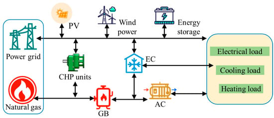
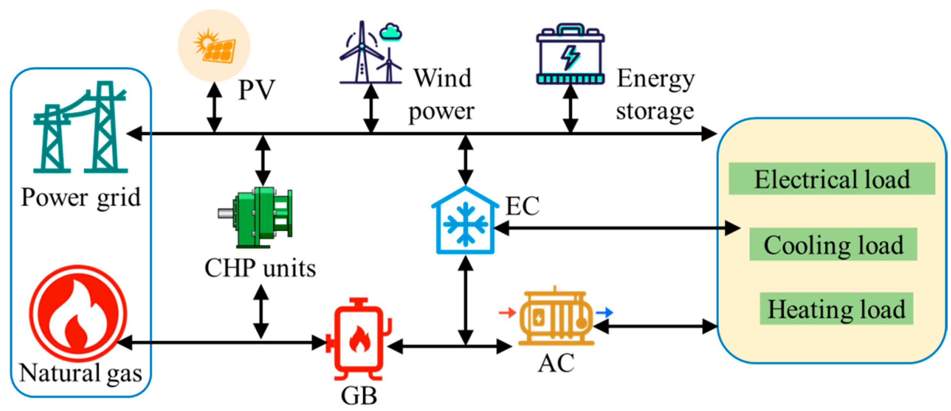
The combined cooling-heating integrated energy system discussed in this paper includes equipment such as Combined Heat and Power (CHP) units, Gas Boilers (GB), Absorption Chillers (AC), and Electric Chillers (EC). Among them, the GB utilizes natural gas for heating; the CHP unit, AC, and EC serve as energy flow coupling devices. The CHP unit generates electricity to meet part of the power demand while utilizing waste heat for heating, achieving electrical-thermal coupling. The AC and EC realize thermal-cooling and electrical-cooling coupling, respectively, enabling the system to meet cooling load demands under different conditions. The various equipment in the system operates collaboratively to provide users with a stable energy supply. The structure of the heating network system is shown in Figure 4. In this paper, a quasi-steady-state method is employed for heat network modeling, without currently taking into account the thermal inertia during the heat fluid transportation process. As a crucial component of a multi-heterogeneous energy system, the core function of heat network modeling is to provide the economic costs, equipment constraints, and energy coupling relationships on the heat side for the game framework, rather than to depict the dynamic fluid characteristics of the heat network itself. If dynamic constraints related to thermal inertia are introduced, a substantial number of state variables in the time dimension and delayed coupling equations will be added to the model, resulting in an exponential increase in its nonlinearity and complexity. From an engineering perspective, the thermal inertia of a heat network primarily depends on the pipeline length and hot water flow velocity. Generally, the transmission delays in urban heat networks mostly range from several minutes to tens of minutes, which are much shorter than the hourly time scale of the planning model in this paper. Within the hourly time dimension, the transmission delay caused by thermal inertia can be considered as instantaneous, and its impact on the hourly energy supply-demand balance, equipment capacity configuration, and economic costs of the heat network can be negligible.

Figure 4. The structure of the heating network system.

To determine the equipment selection and capacity configuration plan for the combined cooling-heating integrated energy system, this paper comprehensively considers the system’s economic costs and aims to minimize the annual comprehensive cost C through optimization. The economic cost is composed of the system’s initial investment cost $C_{inv}$, operational cost $C_{op}$, and maintenance cost $C_{mt}$, with its mathematical representation as follows:

$$\min C=C_{inv}+C_{op}+C_{mt}$$

(30)

Given the impact of the service life of each piece of equipment in the system on the planning scheme, this paper employs the Net Present Value method to convert the initial investment costs of the equipment in the system, expressing them in terms of equivalent annual value:

$$C_{inv}={\displaystyle \sum _{k=1}^m{\lambda }_k{C}_{k,ct}}$$

(31)

Here, m represents the total number of energy equipment types in the system; ${\lambda }_k$ denotes the investment return coefficient for the k-th type of equipment; $C_{k,ct}$ represents the initial investment cost of the k-th type of equipment.

The relevant calculation formulas are as follows:

$${\lambda }_k={\displaystyle \frac{r{(1+r)}^{N_k}}{{(1+r)}^{N_k}-1}}$$

(32)

$$C_{k,ct}=C_{k,build}{x}_{p}p$$

(33)

Here, N_k represents the service life of the k-th type of equipment; r denotes the discount rate; $C_{k,build}$ indicates the unit capacity cost of the k-th type of equipment.

The system operational cost primarily covers the gas consumption cost, and its calculation formula is as follows:

$$C_{op}={\displaystyle \sum _{d=1}^D{\displaystyle \sum _{t=1}^{24}{T}_d(c_{gas}{P}_t^{gas})}}$$

(34)

$$P_t^{gas}=P_t^{GB}{\displaystyle \sum P_{i,t}^{CHP}}$$

(35)

where D represents the number of selected typical days; T_d denotes the number of days in the d-th typical day; $c_{gas}$ indicates the unit purchase price of natural gas, taken as 3.5 yuan/m³, with a heating value of 36 MJ/m³ for natural gas, resulting in a converted $c_{gas}$ of 0.35 yuan/(kW·h); $P_t^{gas}$ represents the gas purchase power during time period t, in kW.

The maintenance cost encompasses various aspects such as equipment repair expenses, spare parts and material costs, monitoring and diagnostic fees, and labor costs. It is calculated based on the initial investment cost, with the calculation formula as follows:

$$C_{mt}=\mu {\displaystyle \sum _{k=1}^m{C}_{k,ct}}$$

(36)

where μ represents the annual maintenance cost coefficient, indicating the proportion of the annual maintenance cost of the equipment to its initial investment cost, and is taken as 0.03.

The constraints for the operation of the heating network mainly include:

(1)

Constraints on CHP Operation

CHP units utilize the waste heat generated during the power generation process to provide heating or meet the thermal energy requirements of industrial processes. A mathematical model is established considering the parameter differences among CHP units:

$$P_{i,e,t}^{CHP}={\eta }_{i,e}^{CHP}{P}_{i,t}^{CHP}$$

(37)

$$P_{i,h,t}^{CHP}={\eta }_{i,h}^{CHP}{P}_{i,t}^{CHP}$$

(38)

where $P_{i,e,t}^{CHP}$ and $P_{i,h,t}^{CHP}$ represent the electrical and thermal power outputs, respectively, of the CHP unit of brand i during time period t, in kW; $P_{i,t}^{CHP}$ denotes the gas consumption power of the CHP unit of brand i during time period t, in kW; ${\eta }_{i,e}^{CHP}$ and ${\eta }_{i,h}^{CHP}$ are the electrical and thermal efficiency, respectively, of the CHP unit of brand i.

(2)

Operational constraints for other energy equipment

As crucial energy flow coupling devices in the system, GB utilizes natural gas as fuel for heating, AC achieves cooling energy supply through absorption and evaporation of refrigerant, and EC employs an evaporation-condensation cycle, driving the compressor with electrical energy for refrigeration. The mathematical models for each piece of equipment are as follows:

$$Q_t^{GB}={\eta }^{GB}{P}_t^{GB}$$

(39)

$$Q_t^{AC}={\eta }^{AC}{P}_t^{AC}$$

(40)

$$Q_t^{EC}={\eta }^{EC}{P}_t^{EC}$$

(41)

where $Q_t^{GB}$, $Q_t^{AC}$ and $Q_t^{EC}$ represent the output powers of GB, AC, and EC, respectively, during time period t, in kW; ${\eta }^{GB}$ denotes the heating efficiency of GB; ${\eta }^{AC}$ represents the energy efficiency ratio of AC; ${\eta }^{EC}$ indicates the coefficient of performance of EC; $P_t^{GB}$ signifies the energy consumption from natural gas combustion in GB during time period t; $P_t^{AC}$ denotes the thermal power consumed by AC during time period t; $P_t^{EC}$ represents the electrical power consumed by EC during time period t.

(3)

Thermal balance constraints

$$P_{heat,t}^{\max }=Q_t^{GB}+{\displaystyle \sum P_{i,h,t}^{CHP}-}{P}_t^{AC}$$

(42)

where $P_{heat,t}^{\max }$ represents the upper limit of the confidence interval for the thermal load in the system during time period t.

(4)

Cooling balance constraints

$$P_{cool,t}^{\max }=Q_t^{EC}+Q_t^{AC}$$

(43)

where $P_{cool,t}^{\max }$ represents the upper limit of the confidence interval for the cooling load in the system during time period t, in kW.

(5)

Equipment output constraints

Considering the equipment model, constraints are imposed on the output of the CHP unit:

$$P_{CHP,i}^{\min }\le P_{i,h,t}^{CHP}\le P_{CHP,i}^{\max }$$

(44)

Affected by the demands for cooling, heating, and electrical loads, the upper and lower output limits of equipment in the system during operation are determined by the planned quantity and operational characteristics of the equipment. This paper imposes constraints on the output ranges of GB, AC, and EC units, with the expressions as follows:

$$\left\{\begin{array}{c}{P}_{\min }^{GB}\le P_t^{GB}\le P_{\max }^{GB}\\ P_{\min }^{AC}\le P_t^{AC}\le P_{\max }^{AC}\\ P_{\min }^{EC}\le P_t^{EC}\le P_{\min }^{EC}\end{array}\right.$$

(45)

The typical scenario generation, equipment planning, and scheduling analysis in this paper are all based on an hourly time scale. However, the variations in Coefficient of Performance (COP) with respect to cooling medium temperature and load rate primarily manifest during real-time operation at the minute/second level. On an hourly time scale, the dynamic fluctuations of COP can be represented by the average COP under rated operating conditions, and its dynamic changes have negligible impacts on the planning aspects such as equipment capacity configuration, annual comprehensive system costs, and energy supply-demand balance. Furthermore, the core task during the planning phase is to determine equipment capacity, installation locations, and the overall economic and technical indicators of the system. Simply calculating the energy conversion relationships and equipment investment and operational costs based on the COP under rated operating conditions is sufficient to meet planning requirements. In contrast, it is necessary to consider the dynamic changes in COP during real-time equipment operation and scheduling to achieve optimized equipment control. Rather than using a uniform, fixed COP value for all representative days, the approach takes into account the characteristic features of typical scenarios generated through deep time clustering, and assigns differentiated COP values based on seasonal variations in ambient temperature. For instance, the rated COP value of refrigeration equipment under high-temperature conditions is selected for typical summer days, while for typical days in winter and transitional seasons, the rated COP values corresponding to their respective temperature ranges are chosen. This ensures that the COP values align with the seasonal environmental characteristics of the typical days.

5. Game-Theoretic Model and Solution Algorithm for Integrated Electrical-Heat Energy Systems

Since the power grid and the heat network belong to different stakeholders, each pursuing the maximization of their economic benefits. If both parties proceed with investment and construction without negotiation, it can easily lead to a waste of resources. To address this, this paper constructs a game-theoretic model for the integrated electrical-thermal energy system, as shown in (46)–(47) below.

$$\min (F*C)$$

(46)

s.t. (20)–(30), (38)–(45)

(47)

The aforementioned optimization model exhibits strong nonlinear and non-convex characteristics, making it difficult for traditional commercial solving software such as CPLEX or Gurobi to efficiently solve the problem. Therefore, this paper employs an improved Firefly Algorithm (FA) to determine the optimal solution.

As a swarm-based intelligent stochastic optimization algorithm, the FA demonstrates higher computational accuracy and faster convergence speed compared to Particle Swarm Optimization (PSO) and Ant Colony Optimization (ACO) algorithms. By simulating the movement characteristics of brighter fireflies attracting each other, the FA algorithm exhibits excellent performance in solving optimization problems.

In the FA algorithm, the direction and distance moved by an individual firefly are determined by the brightness and attractiveness of other fireflies. Initially, the fireflies are randomly distributed in space. Assuming the maximum fluorescence brightness value is I₀ and the maximum attractiveness is τ₀, the calculation methods for the relative fluorescence brightness I and attractiveness τ of a firefly are as follows:

$$I=I_0{e}^{-\gamma d_{ij}}$$

(48)

$$\tau ={\tau }_{0}J(t)e^{-\gamma d_{ij}^2}$$

(49)

Here, γ represents the light absorption coefficient, with γ∈ [0.01,100]; d_ij is the Cartesian distance between firefly i and firefly j; J(t) is the objective function value at the position at time t. The position $X_i(t)$ of firefly i, when attracted by firefly j, is updated as follows:

$$X_i(t+1)=X_i(t)+\tau (X_j(t)-X_i(t))+a({\lambda }_{rand}-0.5)$$

(50)

Here, α is the step size factor, where α ∈ (0, 1); λ_rand is a random perturbation term that prevents the iteration from prematurely converging to a local optimum.

However, the FA algorithm suffers from poor search accuracy in the early stages and is prone to getting trapped in local optima during the later stages of search. Therefore, this paper optimizes the search performance of the algorithm by introducing a mutation mechanism during the movement of individual fireflies. During the movement of individual i, whether mutation occurs is determined by a random mutation coefficient ζ ∈ [0,1]. When ζ < the mutation probability p_m, individual i will undergo mutation, and vice versa. The mathematical expression for the mutation mechanism of individual i is as follows:

$$X_i=X_i+\varphi (\widehat{\Theta }-\underset{⌢}{\Theta })$$

(51)

$$\varphi =\left\{\begin{array}{c}{2}^{{\displaystyle \frac{1}{\eta +1}}-1}, {\xi }_i\le 0.5\\ 1-{[2(1-\xi )]}^{{\displaystyle \frac{1}{\eta +1}}}, others\end{array}\right.$$

(52)

Here, $\widehat{\Theta }$ and $\underset{⌢}{\Theta }$ are the upper and lower limits, respectively, of the independent variables for the constraint function $\varphi$; ${\xi }_i$ ∈ [0,1] is a random number; η is a constant coefficient, set to 20.

The solution process for the power grid optimal dispatch algorithm is as follows: First, generate an initial planning scheme based on regional power grid parameters. Then, substitute the initial scheme into the Improved IFA for iterative optimization, using the reciprocal of its objective function value as the fitness function value. When this value falls below a threshold, the optimal scheme is output. Finally, the power grid will operate according to the optimal scheme, achieving maximum energy consumption through the regulation of units such as energy storage. The power grid and heat network operators engage in a non-cooperative Nash game, achieving equilibrium through a distributed negotiation and iterative bargaining mechanism. They adopt a framework of double-layer nested iteration and IFA. The outer layer transmits boundary parameters and judges convergence, while the inner layer utilizes the IFA for efficient optimization of the non-convex and nonlinear objective functions of both parties. There are inherent differences in the objectives of power grids and heat networks, and they achieve strategy adaptation through interactions of game boundary parameters. The game equilibrium is determined by the fact that if any single entity adjusts its decision variables independently, its own objective function value will deteriorate. Moreover, the objective functions of both exhibit strict monotonicity, with each decision variable corresponding to only one unique objective function value, eliminating the scenario where multiple solutions correspond to the same value. Therefore, the uniqueness of the Nash equilibrium is guaranteed from the perspective of the objective functions.

6. Case Study

6.1. Introduction to the Test System

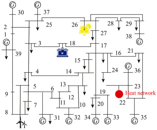
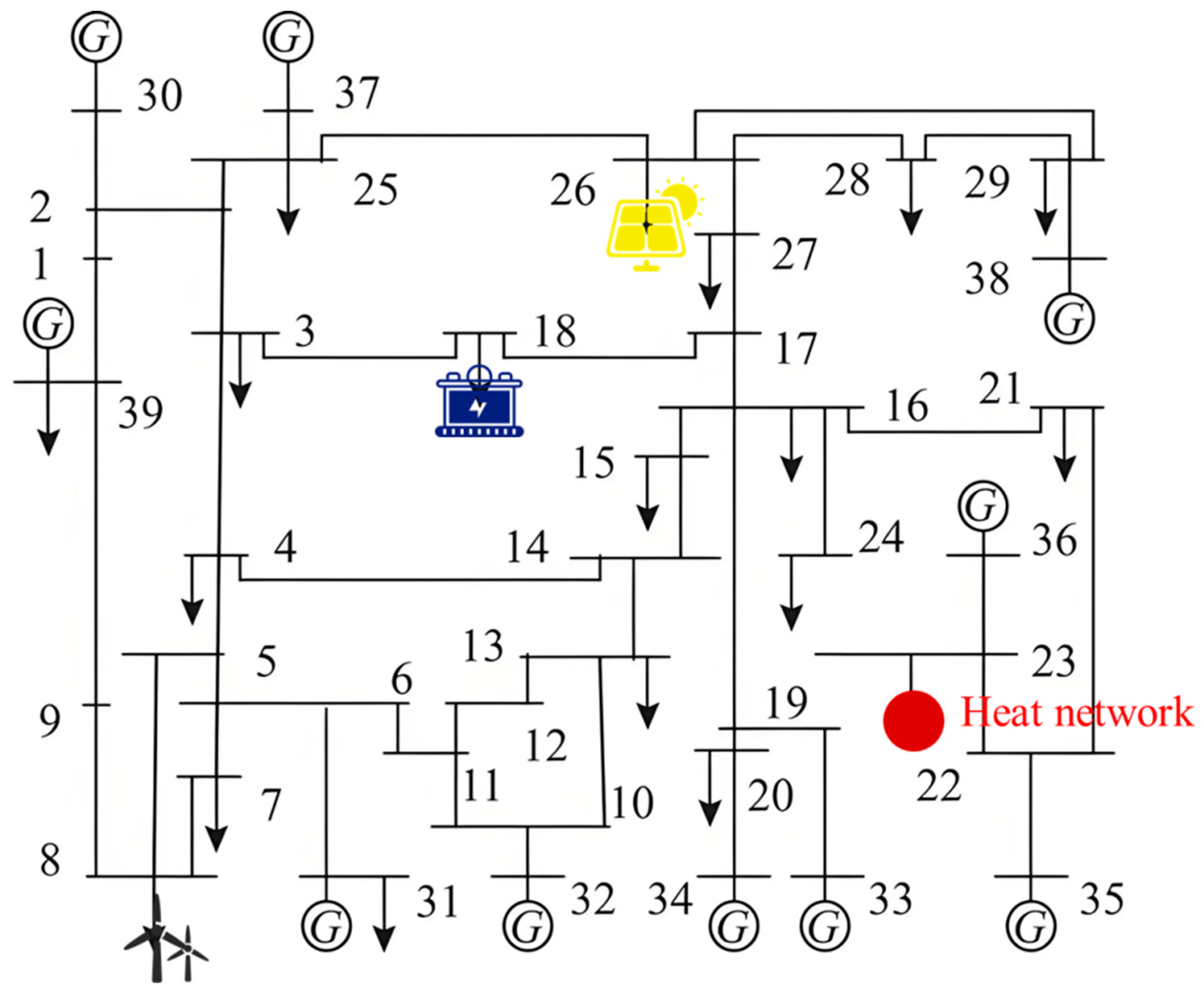
An improved IEEE-39 node test system is employed to validate the effectiveness and feasibility of the proposed method in this paper, with its structural topology depicted in Figure 5 below. In this system, wind turbine generators and photovoltaic power generation equipment are respectively installed at Nodes 8 and 26. Energy storage equipment is installed at Node 18. Additionally, this transmission network incorporates a heat network system, which is connected to the transmission network through Node 22. The detailed structure of the heat network system is shown in Figure 4. The convergence criterion for the game is that the absolute deviation of the power-heat coupling boundary parameters is ≤10⁻⁴ and the relative change rate of the objective function values is ≤1%. In the IFA, the population size is set to 50, the maximum number of iterations is 200, the light absorption coefficient is 0.05, and so on. The upper limit for negotiation iterations is set at 30 rounds.

Figure 5. Structural topology of the improved IEEE-39 node test system.

6.2. Effectiveness Analysis of the Scenario Generation Algorithm

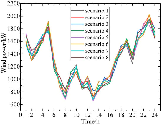
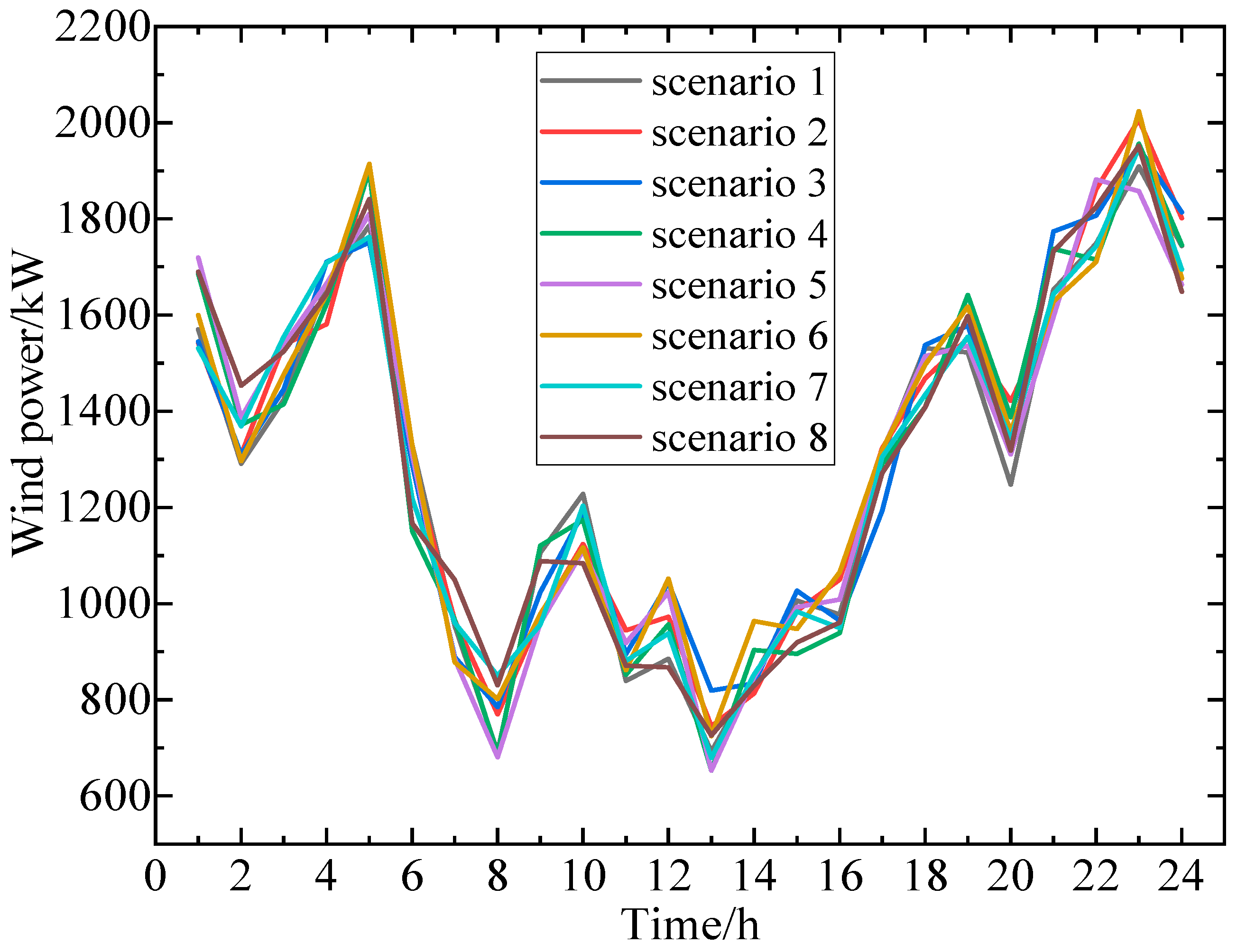
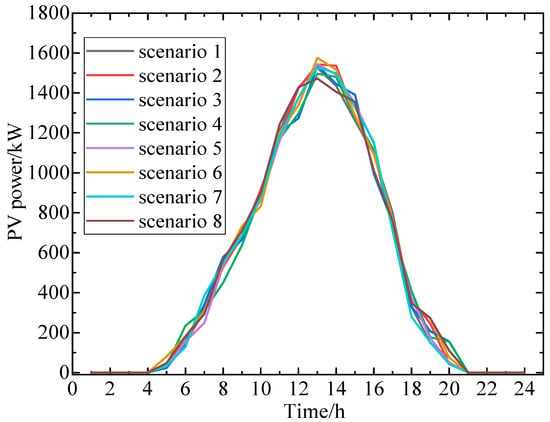
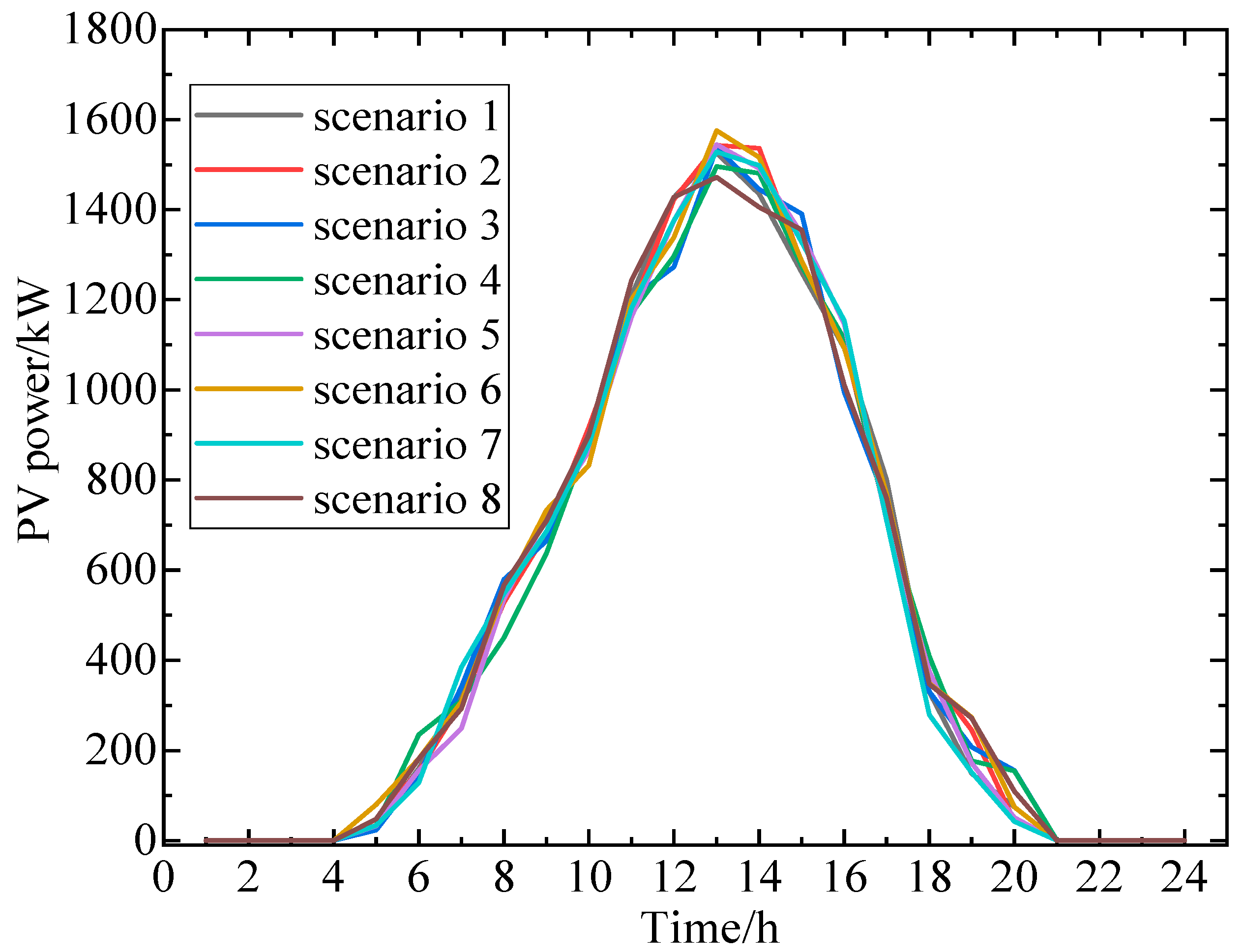
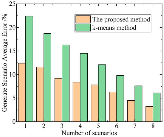
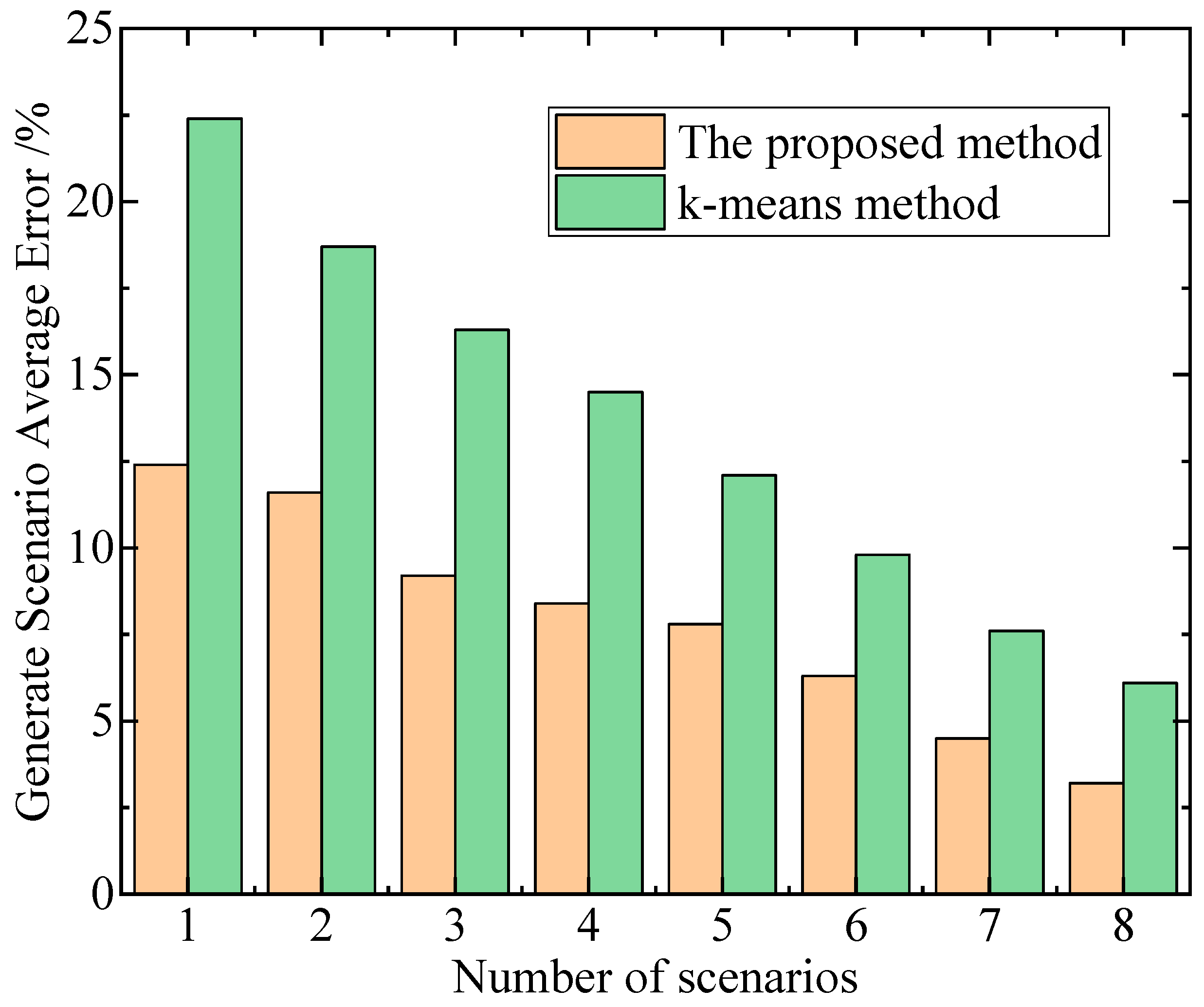
In this paper, the proposed method is employed to generate wind power and photovoltaic output scenarios, with the number of scenarios set to 8. The relevant results are illustrated in Figure 6 and Figure 7. Additionally, the average errors under different numbers of generated scenarios are compared with those obtained using the k-means method, with the results shown in Figure 8.

Figure 6. Generated typical scenarios of the wind power.

Figure 7. Generated typical scenarios of the PV power.

Figure 8. Average errors under different numbers of generated scenarios.

The average error in Figure 8 refers to the average morphological similarity error of temporal data, calculated based on the DTW distance. It serves as a specialized metric for scenario generation in temporal sequences of new energy output. By using the typical scenario sequences generated through clustering as references, the DTW distance between the original sequences and their corresponding typical sequences is calculated, and the arithmetic mean is taken to obtain this average error. It accurately quantifies the degree of fit between the typical scenarios and the morphological characteristics of the original data. A smaller error indicates a higher similarity and a more precise representation of the uncertainty in new energy sources. Unlike the traditional Mean Squared Error (MSE), this metric is more suitable for evaluating temporal clustering scenarios. The longer computation time of the DTC method represents a reasonable cost for achieving accurate feature extraction and scenario generation. Moreover, in long-term electricity-heat planning, its computation time has no practical impact on the planning process, and the computational efficiency can be further optimized in engineering applications.

The deep temporal clustering method can generate typical scenarios that are closer to reality and better describe the uncertainty of new energy output compared to the traditional k-means algorithm and GCAN. This is because the traditional k-means algorithm performs simple clustering solely based on the distances between samples, neglecting the continuity and dynamic variation characteristics of new energy output data in the temporal dimension. Although GCAN may consider certain data structural information, its ability to capture complex temporal dependencies is limited. In contrast, leveraging the powerful nonlinear modeling capabilities of deep neural networks, the deep temporal clustering method can deeply explore the complex patterns, long-term dependencies, and latent temporal dynamic characteristics of new energy output data in time series. Consequently, it can more accurately depict the uncertainty characteristics of new energy output, such as fluctuations and trends, resulting in generated typical scenarios that are more consistent with actual output conditions. Additionally, the deep temporal clustering method exhibits higher computational efficiency because traditional methods like k-means often require manual feature design and have limited ability to capture complex temporal patterns when processing wind and solar new energy output data, leading to the need for multiple iterations and extensive computations to optimize clustering results. In contrast, the deep temporal clustering method utilizes deep neural networks to automatically learn multi-level features and complex temporal dependencies in the data, enabling efficient modeling of the entire time series data in one go. This approach avoids cumbersome feature engineering and repetitive iterative computations while leveraging advantages such as parallel computing to accelerate model training and inference processes, thereby demonstrating higher computational efficiency in generating typical wind and solar new energy output scenarios.

On the other hand, we also compared several other methods for characterizing the uncertainty of new energy output, including robust optimization, fuzzy chance-constrained programming, and the information gap decision theory (IGDT) method. The relevant results are shown in Table 1.

Table 1. Comparison of indicators across different methods.

Method	Total Operating Cost/$	New Energy Accommodation Rate/%	Computational Time/s
The proposed method	14,578	96.3	163.8
Robust optimization method	18,956	91.4	42.3
Fuzzy chance-constrained method	16,254	93.2	47.8
IGDT Method	15,627	94.1	62.3

Through comparison, it can be observed that the method proposed in this paper achieves the lowest total operating cost, albeit requiring longer computational time. The deep temporal clustering method employed in this study can thoroughly explore the complex features and latent patterns of new energy output data in time series, generating highly realistic and diverse typical scenarios. This enables dispatch plans to more precisely align with new energy output, optimize power generation allocation, and effectively reduce total operating costs. However, this method involves training and tuning deep learning models on massive high-dimensional time series data, encompassing numerous data preprocessing and complex computational steps, resulting in relatively long computational times. In day-ahead scheduling, where plans are formulated a day in advance, there is relatively ample time for complex computations, and the primary objective is low-cost operation. The proposed method can meet this critical requirement. In contrast, robust optimization methods adopt conservative dispatch strategies to ensure robustness under the worst-case uncertainty scenarios, leading to excessive reserve capacity allocation and increased operating costs. Fuzzy chance-constrained programming relies on the setting of fuzzy sets, introducing significant subjectivity that may fail to accurately reflect actual uncertainties, resulting in suboptimal dispatch solutions. The IGDT method involves substantial model simplifications when handling complex uncertainties, providing an inadequate depiction of new energy output and also elevating operating costs.

6.3. Analysis of Dispatch Decision-Making Results

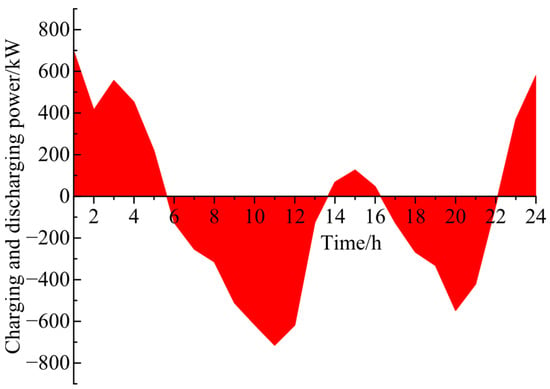
During the dispatch process, the charging and discharging power of the energy storage device is illustrated in Figure 9.

Figure 9. Charging and discharging power of the energy storage device.

In the dispatch of high-proportion renewable energy microgrids, energy storage plays a crucial and multidimensional role. On one hand, due to the intermittency and volatility of renewable energy sources such as wind and solar power, their output is difficult to predict accurately and is unstable. The energy storage system can store excess electrical energy when renewable energy output is surplus and release it when output is insufficient, effectively smoothing out fluctuations in renewable energy output, ensuring the stability and reliability of microgrid power supply, and reducing the risk of power outages or over-reliance on traditional backup power sources caused by unstable renewable energy output. On the other hand, the energy storage system can also participate in peak shaving and valley filling within the microgrid, storing electrical energy during off-peak periods and releasing it during peak periods, thereby reducing the peak load of the microgrid, improving the utilization rate of power equipment, optimizing the allocation of power resources within the microgrid, and simultaneously helping to lower the cost of electrical energy exchange between the microgrid and the main grid, enhancing the economic efficiency of microgrid operation.

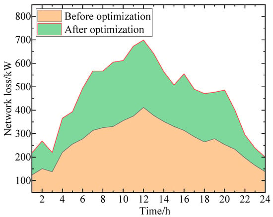
In high-proportion renewable energy power systems, due to the intermittency and volatility of renewable energy generation, its output is difficult to match precisely with load demand in real time, leading to potential unreasonable power flows during transmission. For instance, certain lines may become overloaded during peak renewable energy output periods and underloaded during off-peak periods. This imbalanced power distribution increases resistive losses in lines and iron and copper losses in transformers and other equipment, consequently elevating network losses. The network loss conditions before and after optimization are illustrated in Figure 10. To prevent the planning stage from falling into local optima, three types of core parameter modifications have been made to the IFA: the light absorption coefficient γ is dynamically adjusted with the number of iterations, being large in the initial stage and small in the later stage; a new mutation probability parameter with a value of 0.12 is introduced to randomly mutate individuals with poor fitness; the step-size factor α undergoes piecewise linear optimization, being large in the early stage, moderate in the middle stage, and small in the later stage. Additionally, the population size has been adjusted to 50 and the maximum number of iterations to 200, expanding the initial search base and ensuring fine-grained search and mutation adjustments in the later stages to enhance the effect of preventing local optima.

Figure 10. The network loss conditions before and after optimization.

The energy storage system can store surplus electrical energy when renewable energy generation exceeds demand and grid load is low, and release electrical energy when renewable energy generation is insufficient and grid load is high. By performing peak shaving and valley filling and smoothing out fluctuations in renewable energy output, it enables more stable and orderly power transmission, reduces unreasonable power flows in lines and equipment caused by frequent and significant power fluctuations, lowers the peak and variability of line currents, thereby effectively reducing resistive losses as well as losses in transformers and other equipment, ultimately achieving the goal of reducing network losses.

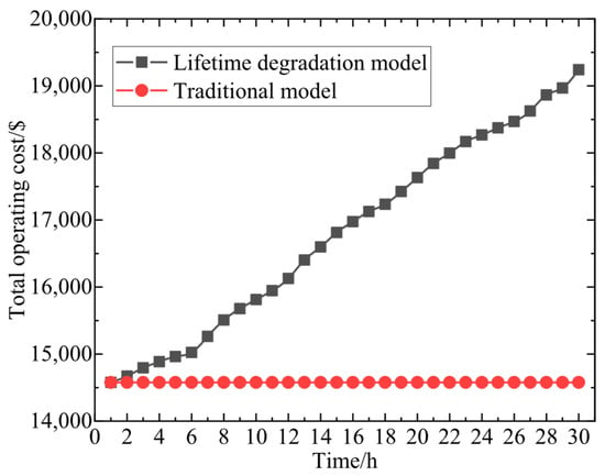
To further illustrate the necessity of accounting for battery life degradation costs, Figure 11 displays the trend of dispatch costs over a month, as shown in Figure 11.

Figure 11. Trend of dispatch costs over a month.

Introducing battery life degradation costs into the objective function to achieve precise accounting of energy storage equipment dispatch expenses offers multiple significant advantages. From an economic perspective, precise accounting of energy storage equipment dispatch costs can more accurately reflect the overall costs of the energy storage system throughout its operational lifecycle, avoiding cost underestimation due to the neglect of battery life degradation costs. This enables microgrid dispatch decisions to be more comprehensive and accurate when considering economic factors, facilitating the formulation of more reasonable electricity pricing strategies and cost-sharing mechanisms, and enhancing the overall economic efficiency of the microgrid. From a technical and management standpoint, it encourages dispatchers to arrange the charging and discharging strategies of energy storage equipment more scientifically and reasonably, preventing damage to battery life caused by unreasonable operations such as overcharging and over-discharging. This extends the service life of energy storage equipment, improves the operational efficiency and reliability of the energy storage system, ensures the long-term stable operation of the microgrid, and achieves coordinated and sustainable development of the new energy microgrid in terms of technology, economy, and environment.

To quantitatively verify the significance of incorporating the cost of battery life degradation into the objective function on the grid side, this section conducts a quantitative analysis through comparative experiments: Two control groups are set up, namely the scenario considering the cost of battery life degradation (denoted as Scenario 1) and the scenario ignoring the cost of battery life degradation (denoted as Scenario 2). Under the same typical renewable energy scenarios, equipment configuration constraints, and game rules, the long-term and short-term operational costs of the two scenarios are quantitatively compared, with the results shown in Table 2.

Table 2. Analysis of the Impact of Battery Life Degradation Cost.

Quantitative Indicators	Scenario 1	Scenario 2
Average Daily Scheduling Cost ($)	452.3	418.7
Average Monthly Battery Life Degradation Cost ($)	685.6	1942.8
Monthly Comprehensive System Benefit ($)	12,568.4	9876.2
Average Daily Charging and Discharging Cycles of Energy Storage	1.2	3.8
SOC Fluctuation Rate of Energy Storage (%)	18.3	47.6
Renewable Energy Consumption Rate (%)	96.3	95.8

When the cost of battery life degradation is ignored, the average daily scheduling cost in Scenario 2 decreases by 7.43% compared to Scenario 1. This is because the scheduling strategy does not need to account for the impact of energy storage charging and discharging on battery life, enabling short-term economic cost minimization through unrestricted charging and discharging operations. However, this strategy results in a 216.67% increase in the average daily charging and discharging cycles of energy storage, a 160.11% intensification in the SOC fluctuation rate, and a staggering 183.36% surge in the average monthly battery life degradation cost compared to Scenario 1. The slight reduction in short-term costs comes at the expense of excessive long-term equipment wear and tear, which violates the whole-life-cycle economic principle of energy system planning. From the perspective of monthly comprehensive system benefits, Scenario 1 achieves a comprehensive benefit of 12,568.4$, while Scenario2 only reaches 9876.2$, representing a decline of 21.42%. This outcome demonstrates that incorporating the cost of battery life degradation into the objective function can, through scientific scheduling, curb ineffective and frequent charging and discharging of energy storage, significantly reduce the whole-life-cycle equipment degradation cost, and generate long-term economic benefits that far outweigh the minor increase in short-term scheduling costs, thereby substantially enhancing the overall economic efficiency of the system.

7. Conclusions

In response to the growing challenges posed by the increasing penetration of renewable energy sources and the complex cooperative-competitive relationships between power grid and heat network operators, this paper has proposed a game theory-based optimal planning strategy for electricity-heat multiple heterogeneous energy systems. By leveraging a deep temporal clustering method, we generated typical scenarios for renewable energy output and utilized energy storage device behaviors to enhance new energy consumption within the distribution system. The integration of battery life degradation costs into the power grid’s objective function allowed for precise accounting of energy storage dispatch expenses, while an optimal dispatch model was established for the heat network side. A game framework was constructed to facilitate decision-making among multiple heterogeneous energy systems, enabling the determination of construction capacity and installation locations for flexible devices under typical multi-scenario conditions. Given the non-convex and nonlinear nature of the model, an improved firefly algorithm was employed to achieve efficient optimal solution search and rapid convergence. Through a case study of an electricity-heat energy system, the effectiveness and feasibility of the proposed method were validated, demonstrating its potential to balance the interests of various stakeholders and enhance the overall planning and operational efficiency of integrated energy systems amidst increasing renewable energy uncertainty.

References

- Huo, Y.; Yang, J.; Qu, J.; Zhang, C.; Zhou, L.; Zhao, W.; Jiang, H.; Wu, Z.; Dai, J.; Duan, W.; et al. Lightweight Data-Driven Planning Method of Hybrid Energy Storage Systems in the New Power System. IEEE Trans. Ind. Appl. 2025, 61, 4792–4800. [Google Scholar] [CrossRef] [Scilit]
- Yan, S.; Shen, Q.; Li, X.; Li, S.; Chu, E. SOC Balancing Control Based on Multi-Agent for Multiple Energy Storage Units in MMC High Power Energy Storage System. CSEE J. Power Energy Syst. 2025, 11, 1253–1261. [Google Scholar]
- Hossain, M.B.; Islam, M.R.; Muttaqi, K.M.; Sutanto, D.; Agalgaonkar, A.P. Component Sizing and Energy Management for a Supercapacitor and Hydrogen Storage Based Hybrid Energy Storage System to Improve Power Dispatch Scheduling of a Wind Energy System. IEEE Trans. Ind. Appl. 2025, 61, 872–883. [Google Scholar] [CrossRef] [Scilit]
- Yang, N.; Lin, D.; Ding, L.; Yang, C.; Zhang, L.; Yang, Y.; Ye, X.; Xiong, Z.; Huang, Y. Optimal Planning for Charging Stations within Multi-coupled Networks Considering Load-Balance Effects. Energy 2025, 336, 138481. [Google Scholar] [CrossRef] [Scilit]
- Liu, Y.; Guan, P.; Sun, L.; Wang, C.; Wang, H. Research on Microgrid Energy Scheduling Strategy Based on Peak-Valley Electricity Pricing and Energy Storage State of Charge (SOC). Electr. Drive 2024, 54, 71–78. [Google Scholar] [CrossRef]
- Wu, H.; Wang, C.; Zuo, Y.; Chen, Y.; Liu, K. Optimization of Home Energy System Based on Time-of-Use Electricity Pricing and Real-Time Control Strategy for Batteries. Power Syst. Prot. Control 2024, 47, 23–30. [Google Scholar]
- Yang, N.; Xiong, Z.; Ding, L.; Liu, Y.; Wu, L.; Liu, Z.; Shen, X.; Zhu, B.; Li, Z.; Huang, Y. A Game-Based Power System Planning Approach Considering Real Options and Coordination of All Types of Participants. Energy 2024, 312, 133400. [Google Scholar] [CrossRef] [Scilit]
- Yang, N.; Hao, J.; Li, Z.; Ye, D.; Xing, C.; Zhang, Z.; Wang, C.; Huang, Y.; Zhang, L. Data-Driven Decision-Making for SCUC: An Improved Deep Learning Approach Based on Sample Coding and Seq2Seq Technique. Prot. Control Mod. Power Syst. 2025, 10, 13–24. [Google Scholar] [CrossRef] [Scilit]
- Bian, A.; Wang, Y.; Luo, Y. A novel chaotic differential variation snake optimization algorithm for parameters estimation of photovoltaic cell and module models. Smart Power Energy Secur. 2025, 1, 133–153. [Google Scholar] [CrossRef] [Scilit]
- Liu, X.; Liu, J.; Zhao, Y.; Ren, K.; Ping, F.; Ding, T. Dynamic Modeling of Gasbag-Structured Compressed Supercritical Carbon Dioxide Energy Storage. IEEE Trans. Sustain. Energy 2025, 16, 2251–2254. [Google Scholar] [CrossRef] [Scilit]
- Li, P.; Zhou, Z.; Cha, C. Lightning Overvoltage Analysis of Photovoltaic-energy Storage Hybrid System Connected to Distribution Line. High Volt. Appar. 2025, 61, 202–208. [Google Scholar] [CrossRef]
- Wang, B.; Zhang, C.; Dong, Z.Y.; Li, X. Improving hosting capacity of unbalanced transmission networks via robust allocation of battery energy storage systems. IEEE Trans. Power Syst. 2021, 36, 2174–2185. [Google Scholar] [CrossRef] [Scilit]
- Yang, N.; Shen, X.; Liang, P.; Ding, L.; Yan, J.; Xing, C.; Wang, C.; Zhang, L. Spatial-temporal Optimal Pricing for Charging Stations: A Model-Driven Approach Based on Group Price Response Behavior of EVs. IEEE Trans. Transp. Electrif.s 2024, 10, 8869–8880. [Google Scholar] [CrossRef] [Scilit]
- Sharma, S.; Niazi, K.R.; Verma, K.; Rawat, T. Coordination of different DGs, BESS and demand response for multi-objective optimization of transmission network with special reference to Indian power sector. Int. J. Electr. Power Energy Syst. 2020, 121, 106074. [Google Scholar] [CrossRef] [Scilit]
- Zheng, G.; Nan, Y.; Meng, F.; Shen, J.; Lu, Z.; Han, Y. Hierarchical Optimal Schedule for Active Distribution Network Considering Energy Storage System and Distribution Network Reconfiguration. High Volt. Appar. 2025, 61, 53–63. [Google Scholar] [CrossRef]
- Wu, Y.; Yao, L.; Liao, S.; Liu, Y.; Li, J.; Wang, X. A Distributed Photovoltaic-Energy Storage Aggregation Peak Shaving Method Based on an Improved K-means++ Algorithm. Power Grid Technol. 2022, 46, 3923–3931. [Google Scholar]
- Das, C.K.; Bass, O.; Kothapalli, G.; Mahmoud, T.S.; Habibi, D. Overview of energy storage systems in transmission networks: Placement, sizing, operation, and power quality. Renew. Sustain. Energy Rev. 2018, 91, 1205–1230. [Google Scholar] [CrossRef] [Scilit]
- Saxena, A.; Shankar, R. An Interactive Operating Demand Response Approach for Hybrid Power Systems Integrating Renewable Energy Sources. Prot. Control Mod. Power Syst. 2024, 9, 174–194. [Google Scholar] [CrossRef] [Scilit]
- Zafar, R.; Ravishankar, J.; Fletcher, J.E.; Pota, H.R. Optimal dispatch of battery energy storage system using convex relaxations in unbalanced distribution grids. IEEE Trans. Ind. Inform. 2019, 16, 97–108. [Google Scholar] [CrossRef] [Scilit]
- Zhu, J.; Liu, Y.; Xu, L.; Jiang, Z.; Lin, X. Adjustable Robust Optimal Configuration of Energy Storage in Transmission networks with Full Wind Power Accommodation. Power Grid Technol. 2018, 42, 1875–1883. [Google Scholar]
- Zeng, Y.; Yang, Q.; Lin, Y.; Chen, Y.; Chen, X.; Wen, J. Fractional-order virtual inertia control and parameter tuning for energy-storage system in low-inertia power grid. Prot. Control Mod. Power Syst. 2024, 9, 70–83. [Google Scholar] [CrossRef] [Scilit]
- Yang, N.; Xu, G.; Fei, Z.; Li, Z.; Du, L.; Guerrero, J.M.; Huang, Y.; Yan, J.; Xing, C.; Li, Z. Two-Stage Coordinated Robust Planning of Multi-Energy Ship Microgrids Considering Thermal Inertia and Ship Navigation. IEEE Trans. Smart Grid 2025, 16, 1100–1111. Available online: https://ieeexplore.ieee.org/document/10834446 (accessed on 13 March 2026). [CrossRef] [Scilit]
- Zhang, D.; Saif, M.; Jiang, S.; Wang, L.; Liu, J.; Chen, Y.; Li, M. An Optimal Configuration Method for Energy Storage Systems in Photovoltaic Power Plants Based on Probabilistic Power Flow. Energy Storage Sci. Technol. 2021, 10, 2244–2251. [Google Scholar]
- Chen, X.; Liu, L.; Kang, X.; Ma, X.; Li, X.; Li, S.; Zhao, B.; Zhang, Y.; Liu, X. Three-layer game multi-objective optimization scheduling strategy of integrated energy systems considering the ULDs. Smart Power Energy Secur. 2025, 1, 154–164. [Google Scholar] [CrossRef] [Scilit]
- Chen, Z.; Zhang, X.; Wang, X.; Peng, L.; Wen, W.; Liang, W.; Lin, S. A Distributionally Robust Optimization Configuration Method for Distributed Photovoltaic Power Plants Integrated into Transmission networks. Power Syst. Prot. Control 2021, 49, 30–42. [Google Scholar]
- Zhang, Y.; Zhang, S.; Liu, S.; Yi, Y. Bi-Level Planning for Distribution Transformers Considering the Integration of Distributed Photovoltaic and Energy Storage. Power Syst. Prot. Control 2020, 48, 9–15. [Google Scholar]
- Li, Y.; Wang, J.; Cao, X.; Zhou, B.; Lu, S. A Chance-Constrained IGDT Model for Joint Planning of Wind Farms, Energy Storage, and Transmission Networks. Power Grid Technol. 2019, 43, 3715–3724. [Google Scholar]
Disclaimer/Publisher’s Note: The statements, opinions and data contained in all publications are solely those of the individual author(s) and contributor(s) and not of MDPI and/or the editor(s). MDPI and/or the editor(s) disclaim responsibility for any injury to people or property resulting from any ideas, methods, instructions or products referred to in the content. |
© 2026 by the authors. Licensee MDPI, Basel, Switzerland. This article is an open access article distributed under the terms and conditions of the Creative Commons Attribution (CC BY) license.