


Abstract
Lost Circulation (LC) is one of the most common and high-risk complex situations encountered during drilling operations, posing a serious threat to the safe extraction and economic viability of oil and gas resources. Traditional wellbore leakage detection methods based on human experience often suffer from delays and uncertainties, making it difficult to meet real-time warning requirements under complex geological conditions. This paper proposes an LC warning method that combines a physical model with a combination of neural networks (Crested Porcupine Optimizer (CPO)–Long Short-Term Memory (LSTM)–Random Forest (RF)). The physical model utilises changes in mud pit volume, inlet–outlet flow rate differences, and riser pressure to construct interpretable event labels, thereby enhancing the physical plausibility of prediction results. The deep learning component employs LSTM networks to extract temporal features and RF for non-linear discrimination and introduces the CPO algorithm for feature selection and hyperparameter optimisation, thereby enhancing the model’s stability and generalisation capability. Validation using actual field data from the western Bohai Bay oilfield demonstrates that the proposed method outperforms traditional models in accuracy, precision, recall, and F1-score. It also offers a significant improvement in early warning time, detecting potential leakage about 17 min before traditional methods. These results highlight the effectiveness of the approach in managing risks during drilling operations.
1. Introduction
LC is one of the most common and risky complex situations in drilling engineering, which may lead to drilling fluid loss, well control failure, or even blowout accidents [1]. Due to the limitations of existing drilling technologies, as drilling advances into deeper and more complex formations, the frequency and severity of LC incidents continue to increase, placing higher demands on safety and economic efficiency [2]. Therefore, the development of real-time, reliable wellbore leakage warning technologies is of great significance.
During oil extraction, changes in mud pit volume are typically used to determine operating conditions and predict abnormal events. These changes are closely related to drilling risks, and the occurrence of LC can cause significant changes in mud parameters. During drilling operations, variations in mud pit volume are commonly monitored to evaluate operating conditions and detect abnormal events [3]. Such variations are strongly associated with drilling risks [4], as LC typically induces significant fluctuations in mud-related parameters [5]. However, traditional manual LC identification still relies on a few individual indicators and the subjective judgment of personnel, which often leads to delayed or inaccurate detection, limited reproducibility, and inadequate reliability for on-site LC management in complex field environments.
With the rapid development of computer technology, machine learning technology has been widely applied in various fields such as engineering and medicine [6,7,8]. Precise identification of LC based on engineering data and machine learning (ML) has become a research hotspot. Convolutional neural networks (CNNs), RF, support vector machines (SVMs), and artificial neural networks (ANNs) are among the various ML and Deep learning (DL) methods that have been widely applied. These models typically use drilling parameters and geological information as input and can provide early warning for LC to a certain extent. As research continues to advance, related methods have evolved from early single artificial neural networks to more complex implementations such as convolutional neural networks and multi-model fusion, significantly improving the accuracy and real-time performance of predictions. Table 1 summarises the relevant model studies on LC.
Table 1.
Related algorithm research.
Existing data-driven LC warning models primarily rely on statistical correlations and lack explicit process-level constraints, which may lead to physically inconsistent predictions and delayed alarms under complex drilling conditions. To address this gap, this study proposes a physics-constrained hybrid early-warning framework that explicitly integrates physical consistency criteria into the learning and optimization process, enabling both accurate and timely LC prediction. By integrating physical principles with machine learning, it is possible to ensure that predictive outcomes not only exhibit high accuracy but also align with actual physical phenomena, thereby enhancing the model’s reliability and practical value.
To this end, this paper proposes an LC early warning framework that combines physical constraints with a combinatorial neural network. Physical constraint labelling system: Based on changes in mud pit volume, inlet–outlet flow rate differences, and riser pressure, wellbore leakage criteria are established to ensure that prediction results comply with physical laws and field experience. The CPO–LSTM–RF model utilizes LSTM to extract temporal features, RF for nonlinear discrimination to enhance robustness, and CPO for feature selection and hyperparameter optimization to improve stability. By coupling physical knowledge with optimized data-driven learning, the proposed method aims to achieve both interpretability and high predictive accuracy in LC early warning.
2. Materials and Methods
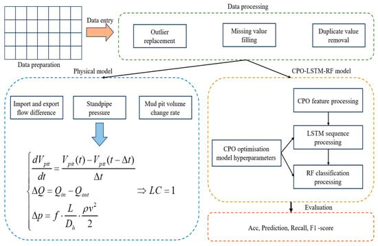
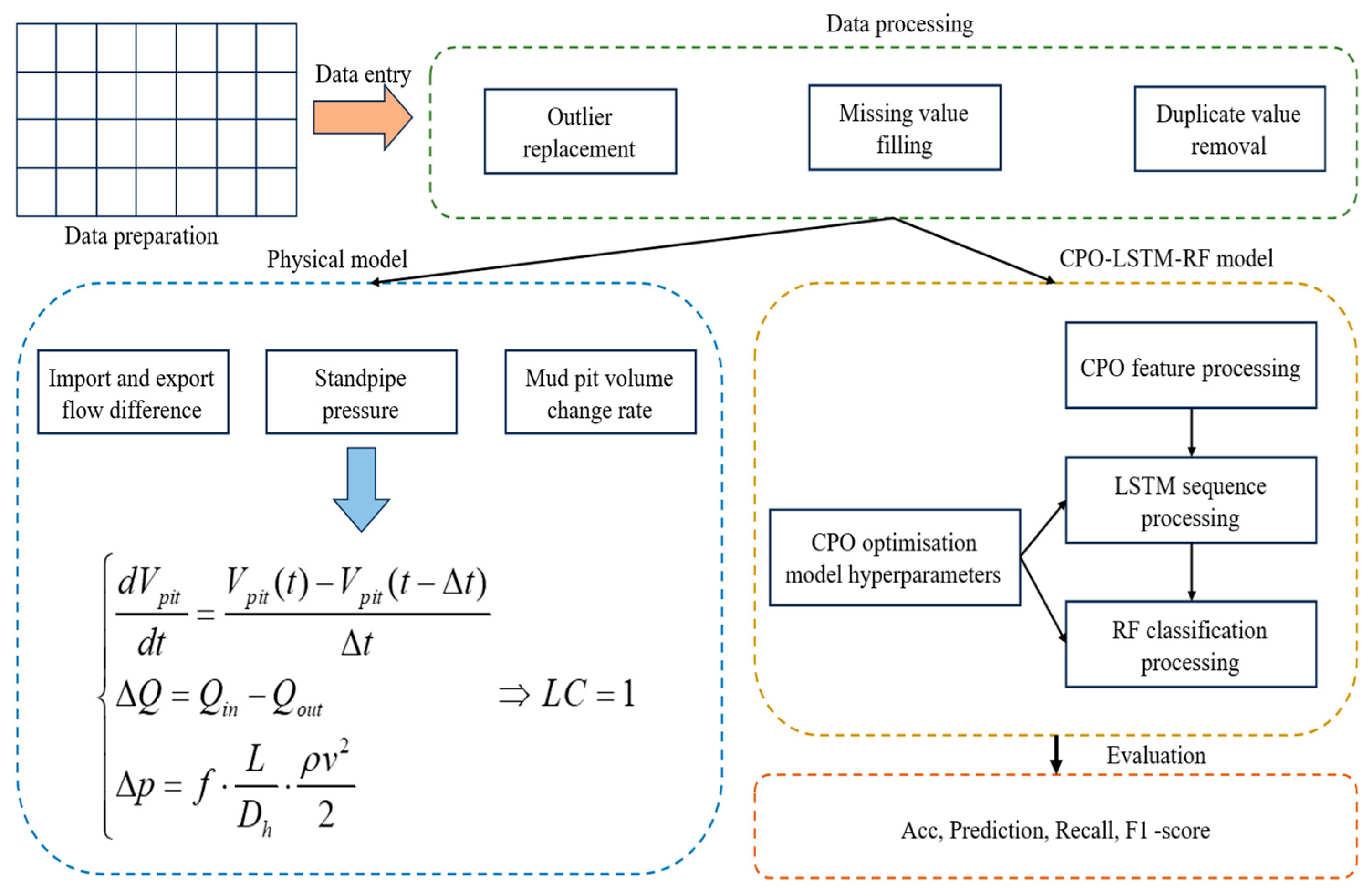
The overall framework of the proposed LC early warning method is illustrated in Figure 1. The workflow consists of five main stages: data preparation, data processing, physical model, CPO-LSTM-RF model, and evaluation.
Figure 1.
Early warning model process for LC based on physical models and combined neural network processes.
- (1)
- Data preparation and processing—Drilling data from multiple sensors at X oilfield is first collected and standardised. To ensure data quality, pre-processing steps such as outlier replacement, missing value interpolation, and duplicate value deletion are applied, ultimately generating a consistent and reliable dataset.
- (2)
- Physical model—To enhance interpretability, physically meaningful features are constructed from drilling hydraulics, including mud pit volume change rate, inlet–outlet flow difference, and standpipe pressure variation. These parameters are embedded into the dataset both as labeling criteria and as input features, ensuring that the learning process adheres to fluid continuity and wellbore pressure balance principles.
- (3)
- CPO–LSTM–RF model—The processed dataset is then fed into the proposed hybrid framework. Specifically, the CPO performs feature selection and hyperparameter optimization; the LSTM module captures temporal dependencies in drilling sequences; and the RF classifier enhances nonlinear discrimination and robustness against noise.
- (4)
- Evaluation—Finally, the model outputs LC risk predictions, which are quantitatively assessed using accuracy, recall, F1-score, and related performance indicators, providing a comprehensive evaluation of model effectiveness.
This integrated workflow enables the proposed method to combine the strengths of physics-informed modeling and data-driven learning, thereby improving both predictive accuracy and engineering applicability.
2.1. Data Processing
The dataset used in this study was obtained from the X oilfield in the western Bohai Bay, China. Due to the complex geological conditions in this area, drilling operations are frequently affected by complications such as LC and blowouts [17]. LC events not only disrupt drilling operations and increase costs, but also pose serious safety and environmental risks. This dataset comprises records from ten wells, with a sampling frequency of 1 s, totalling 40,827 samples organised by well section. Representative LC cases are detailed in Table 2. The training and test datasets in this study are allocated at a ratio of 7:3. To enhance the model’s robustness, the training data primarily comprises data from neighbouring well sections or geological conditions exhibiting similar characteristics.
Table 2.
Some LC records.
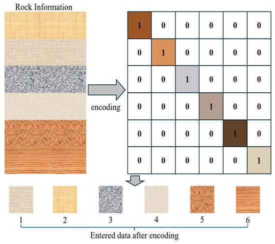
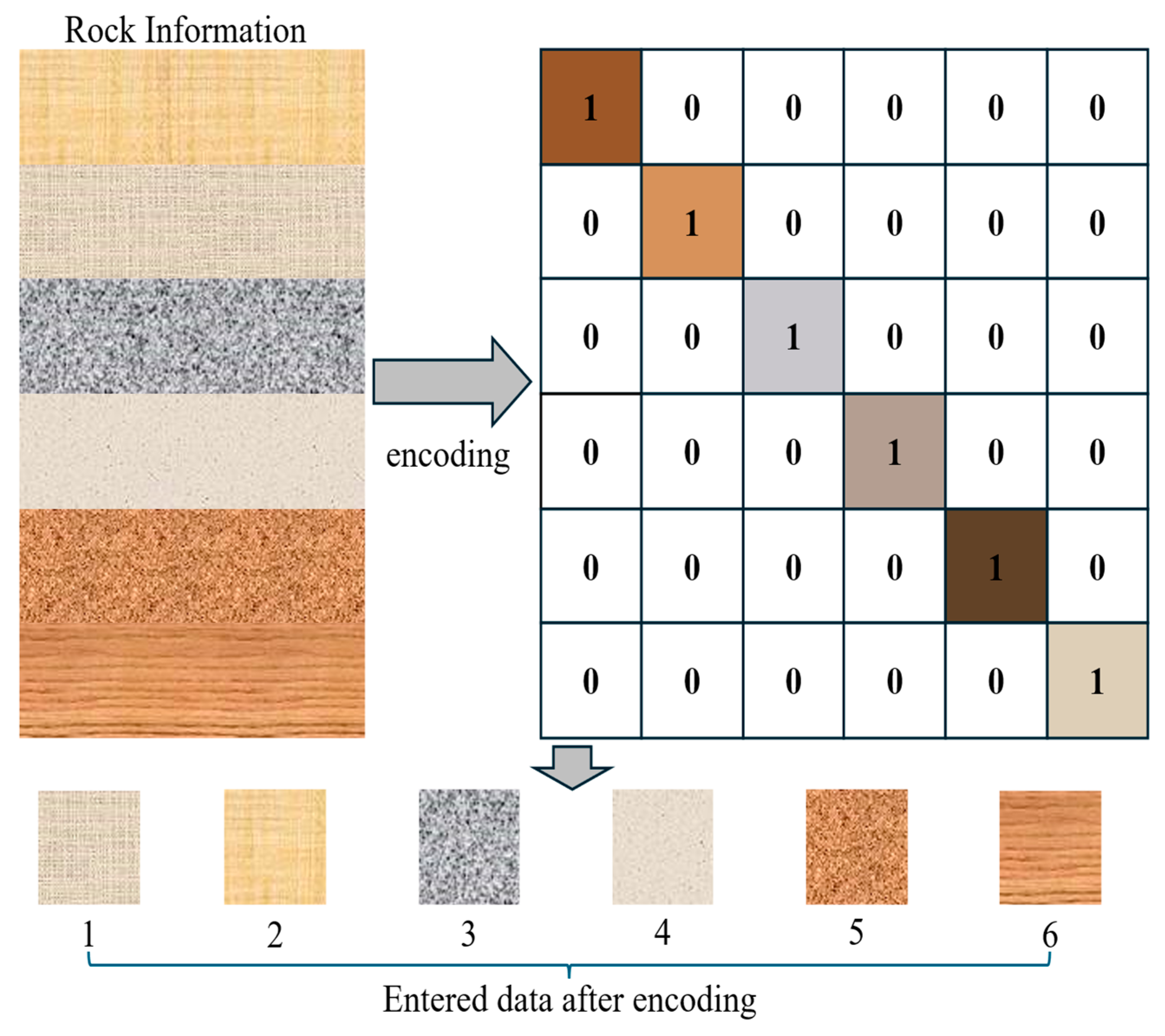
The foundation of LC early warning lies in the effective utilization and structured representation of multi-source drilling data. Such data can be broadly categorized into dynamic and static characteristics. Dynamic characteristics are real-time engineering parameters with high sampling frequency, such as pump pressure, standpipe pressure, rate of penetration, and flow in/out. Static characteristics, in contrast, remain relatively stable over short time periods and include formation properties (e.g., lithology, porosity, permeability) and drilling fluid parameters (e.g., density, viscosity). Static data consists of parameters expressed in natural language, thus necessitating the encoding of such data, as illustrated in Figure 2. Notably, in fractured formations, a high probability of LC may persist even when dynamic parameters exhibit only minor fluctuations, underscoring the necessity of integrating both dynamic and static features. The statistical variables employed in this study are summarized in Table 3.
Figure 2.
Static data encoding process.
Table 3.
Statistical parameters.
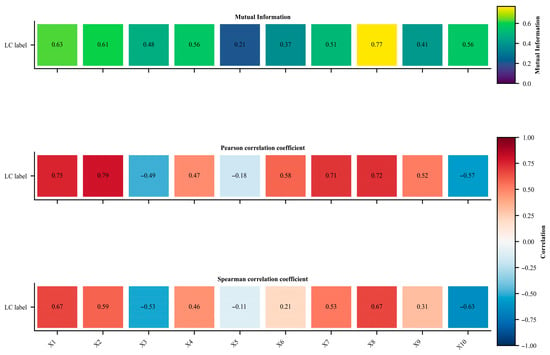
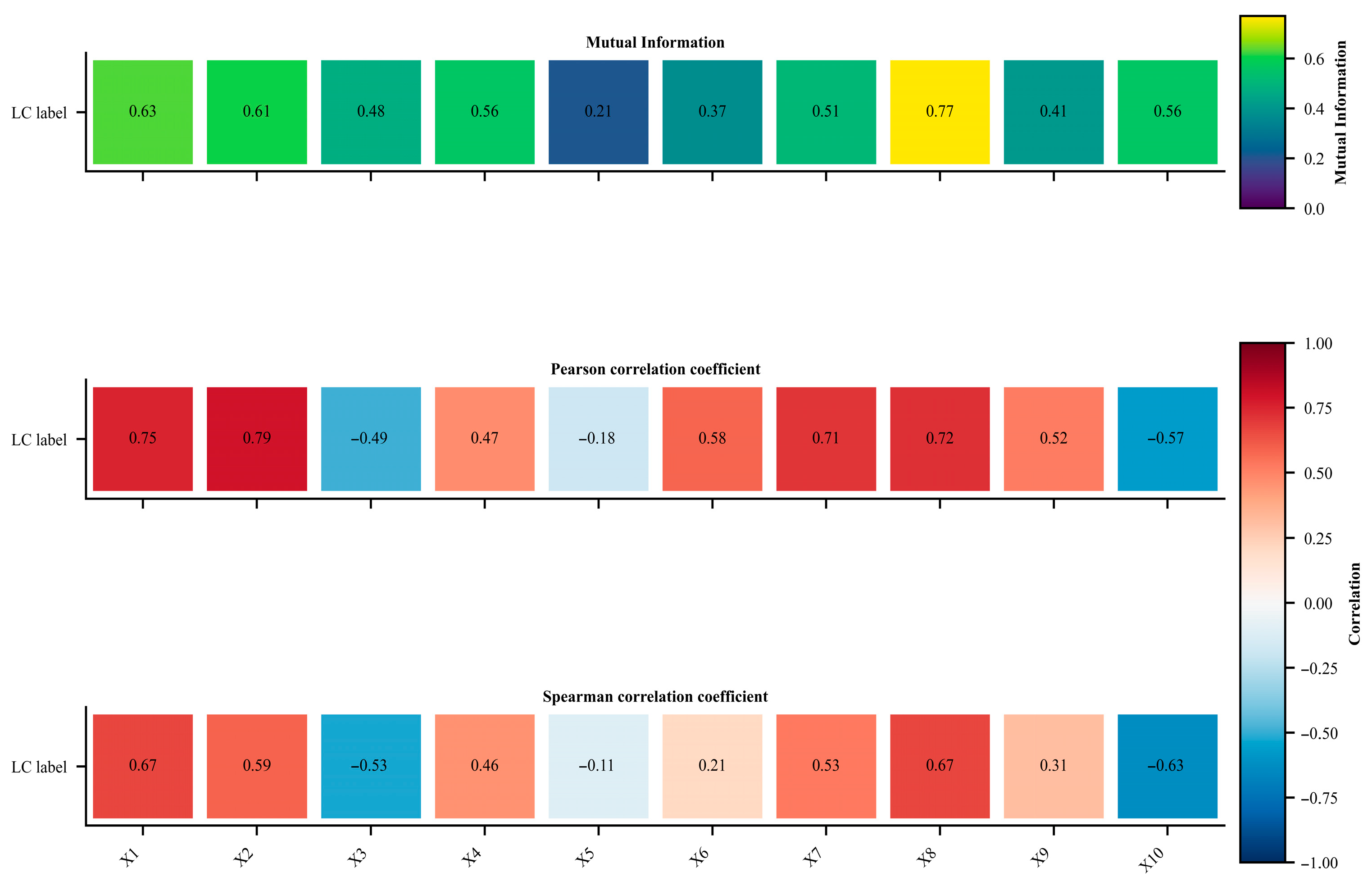
The features statistically analysed in this paper provide useful a priori information for LC risk assessment. However, some features are still unrelated to LC. To improve the robustness of the model, it is essential to perform correlation analysis to eliminate irrelevant and useless features. This paper employs commonly used methods including mutual information analysis, Pearson correlation analysis, and Spearman correlation analysis to conduct feature correlation analysis on these eigenvalues [18,19,20]. The results are presented in Figure 3.
Figure 3.
Results of the correlation analysis.
Based on the results of the correlation analysis and the limitations of actual field application, this study excluded certain correlation coefficients and input parameters, as shown in Table 4.
Table 4.
Input parameters.
During drilling operations, engineering parameters are typically collected in real time through sensors installed at the wellhead and downhole. However, the prolonged duration of drilling, complex operating conditions, and variable environments inevitably lead to data quality issues, including outliers and missing values. These problems may arise from sensor accuracy limitations, equipment malfunctions, signal attenuation in harsh downhole environments, or operational fluctuations during drilling. Such anomalies and data gaps compromise the integrity of raw records and may introduce biases in subsequent analysis, pattern recognition, and predictive modeling, thereby reducing the reliability of downhole condition assessment and decision support. To address these challenges, quality control procedures were applied during data preprocessing, including noise filtering, anomaly detection, and interpolation-based reconstruction, to optimize the completeness and reliability of the dataset.
To ensure temporal consistency of dynamic monitoring data across multiple parameters, this study first aligned the timestamps of drilling construction data so that the sampling times of each sensor strictly corresponded to each other. On this basis, missing values and outliers were handled in a layered manner.
To reduce the impact of sensor failures, communication interruptions, and environmental interference on data quality, abnormal values are detected by calculating the mean and standard deviation using a sliding window [21].
where represents the window; and represent the sample mean and standard deviation within the window, respectively; and represents the threshold coefficient. Data identified as abnormal will be marked as missing values and included in the subsequent imputation process.
For missing data, a graded processing strategy is adopted based on the duration of the missing data:
- (1)
- Short-term continuous absence (<10 s)
Linear interpolation is used to fill in missing values in order to maintain data continuity and smoothness [22]. The calculation formula is shown in Equation (2).
where t represents the time point of the missing data, u and t are the time points of the previous data, and are the values at time points u and v, is the current interpolation.
- (2)
- Long-term gaps (>10 s)
The missing segments are completed using a state estimation method based on Kalman filtering [23]. This method utilises the system state space model and historical observation data to perform optimal interpolation of the missing segments in terms of minimum mean square error.
To accelerate model convergence and eliminate the influence of different features, normalisation is an essential step [24]. Common normalisation methods include minimum–maximum normalisation and Z-score standardization [25]. Since the dataset range is known and contains a few outliers, minimum–maximum normalisation is used to process the data, with the calculation formula shown in Equation (3). Data augmentation is applied to the dataset to enhance the accuracy of model predictions, with the process illustrated in Figure 4.
where is the max–min normalised result for the i-th variable, is the original i-th variable, is the minimum value of the original i-th variable, and is the maximum value of the original i-th variable.
Figure 4.
Data set sample expansion.
2.2. Physical Model
The mechanism behind LC occurrence is complex, and changes in a single parameter cannot uniquely determine its occurrence. Therefore, multiple monitoring parameters must be integrated to identify LC. In this study, an LC event label was established based on physical monitoring parameters and engineering experience, which was used to train and evaluate supervised deep learning models. This label system not only reflects the occurrence and development of LC but also ensures that model outputs can be directly mapped to on-site operational recommendations, thus enhancing the engineering applicability and interpretability of the prediction results. Currently, LC event identification primarily relies on three categories of real-time drilling parameters: mud pit volume, inlet/outlet flow rate, and riser pressure [2].
The rate of change in mud pit liquid level () is calculated over a time interval of length to determine the rate of change in active mud pit volume. A sustained decrease in liquid level over a short period of time typically indicates drilling fluid leakage into the formation [26]. The calculation formula is shown in Equation (4).
where is the volume of the mud pit at time t.
represents the difference between the inflow and outflow rates of drilling fluid, which is one of the most critical real-time monitoring indicators for determining LC [27]. represents normal drilling in this process, with no error between the inflow and outflow rates. > 0 indicates that some drilling fluid has intruded into the formation and has not returned to the wellhead, which may cause a well leak. The calculation formula is shown in Equation (5).
where represents the drilling fluid flow rate pumped into the wellbore in real time, and represents the drilling fluid flow rate returning from the wellhead.
In wellbore leakage warning modelling, changes in can reflect the pressure transmission characteristics of the circulation system. If an abnormal decrease occurs under the same pumping rate and wellbore conditions, it may indicate that drilling fluid has entered the formation, thus serving as an important criterion for wellbore leakage [28]. Under stable circulation conditions, the equation for calculating the pressure drop in the annulus is shown in Equation (6).
where is the friction coefficient, is the wellbore length, is the hydraulic diameter, is the drilling fluid density, and is the annular flow velocity.
In this study, and are defined as the criteria boundaries for wellbore leakage. These thresholds are not fixed but can be adjusted according to different well types and formation characteristics. Their values are based on the statistical distribution of historical downhole operation data, with the 95th percentile value of flow fluctuations under normal circulation conditions selected as the threshold.
Combining the above three types of monitoring parameters with seepage mechanisms, criteria for identifying well leaks can be established:
where represents that a wellbore leak event has occurred.
This criterion provides a physical basis for label construction in supervised learning models, ensuring that early warning results are both data-driven and consistent with engineering principles, thereby enhancing the reliability and interpretability of the model.
In summary, the core logic of this physical rule is to convert multi-source monitoring signals (volume, flow rate, pressure) into a binary physical label (1 = LC, 0 = normal). This label construction strictly adheres to the fundamental engineering principle that ‘mass loss accompanies pressure anomalies’, thereby providing a training objective for subsequent supervised learning models that combines physical consistency with interpretability. This physical model can be employed independently for real-time computation and monitoring, or function as a feature extraction module. Its output—dynamic physical features ()—can be fed alongside raw sensor data into the CPO-LSTM-RF hybrid model to further enhance the accuracy and robustness of early warnings. This physical model can be implemented for real-time calculation and monitoring in the field, and can also serve as a feature extraction module, feeding dynamic features into the CPO-LSTM-RF to further improve the accuracy and robustness of early warning for LC.
2.3. CPO-Optimized LSTM–RF Hybrid Model
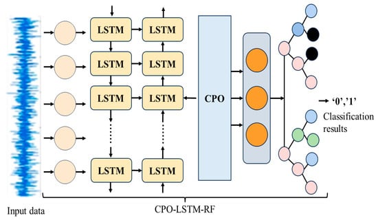
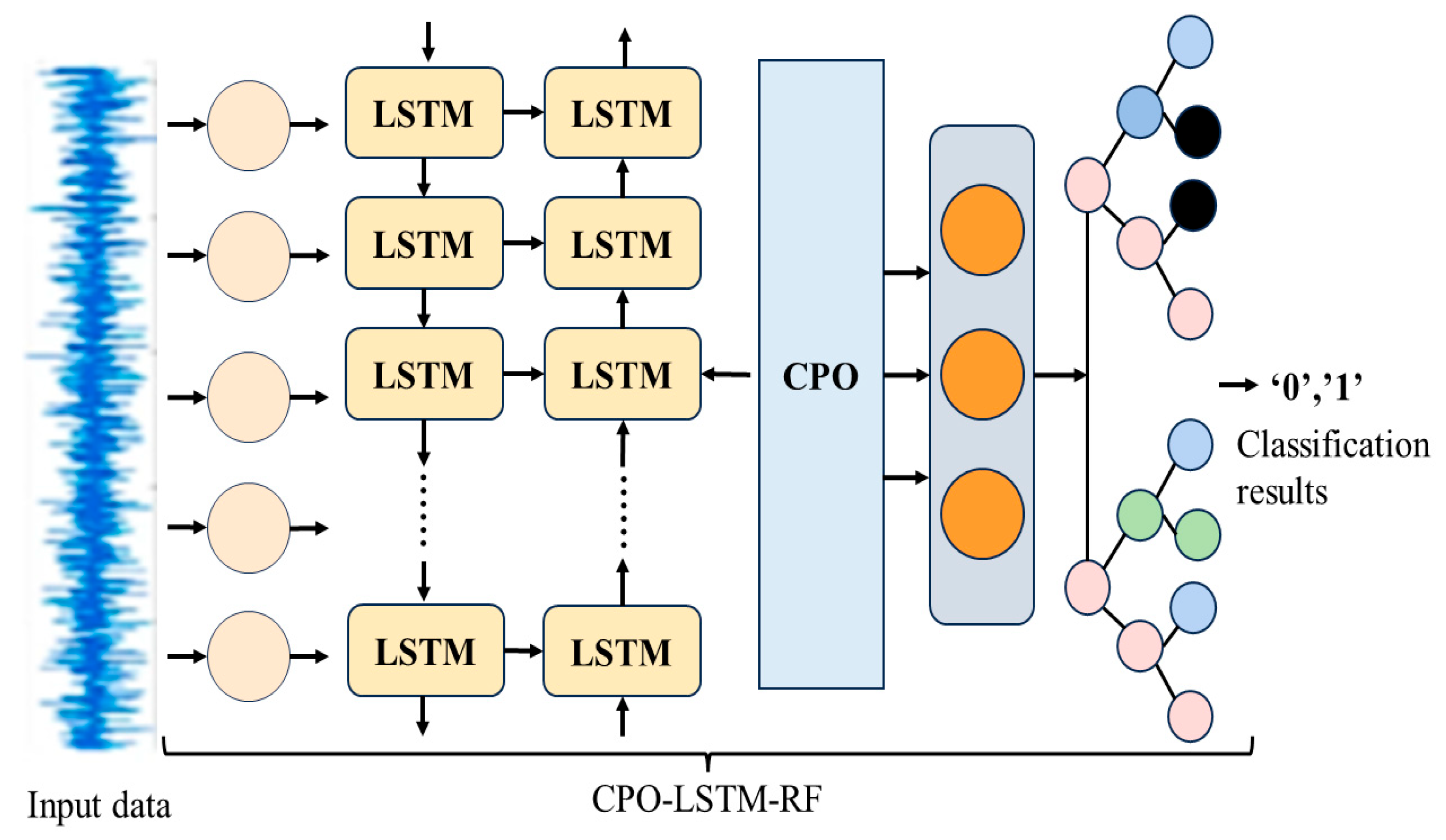
This study proposes a combined neural network framework that combines the advantages of RF in processing linear features with the ability of LSTM to capture non-linear time series patterns, and introduces CPO to enhance the feature selection and modelling capabilities of LSTM. The specific process is shown in Figure 5.
Figure 5.
CPO-LSTM-RF structure.
The hybrid model is divided into three consecutive stages:
In the first stage, features are extracted from drilling operation information. Dynamic data includes time series such as pump pressure, riser pressure, backpressure, and changes in mud pit liquid level; static data includes engineering parameters such as well type, wellbore diameter, casing programme, mud system, and formation type. Unlike traditional methods that rely solely on a single measurement signal, this stage performs feature engineering on multi-source data, converting it into multi-dimensional feature vectors suitable for LSTM input, thereby capturing more potential signals before LC occurrence.
In the second stage, a specially designed LSTM network is used for deep modelling of time-series features to accurately identify long-term dependency patterns in the drilling process. This structure includes two stacked LSTM layers for extracting higher-order temporal relationships; a Dropout mechanism is introduced between layers to suppress overfitting. Additionally, two fully connected layers are set up for specific LC risk classification tasks. In this framework, the softmax output layer of the traditional LSTM is replaced by a RF classifier, enabling the model to achieve more robust nonlinear classification based on feature fusion.
In the third stage, the CPO algorithm is introduced in the model optimisation process to enhance the model’s generalisation capability. Specifically, CPO performs global search and filtering on the output features of the first fully connected layer (FC1), identifying the most discriminative feature subset for LC prediction, and inputs it into the RF classifier for final prediction. This mechanism ensures that the model maintains computational efficiency while utilising the most information-rich features, thereby improving the accuracy and reliability of early warning for LC.
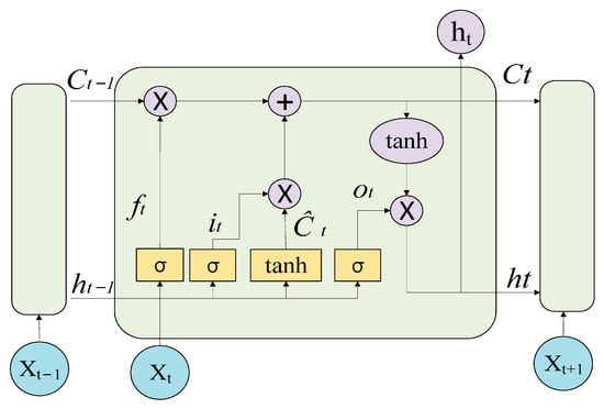
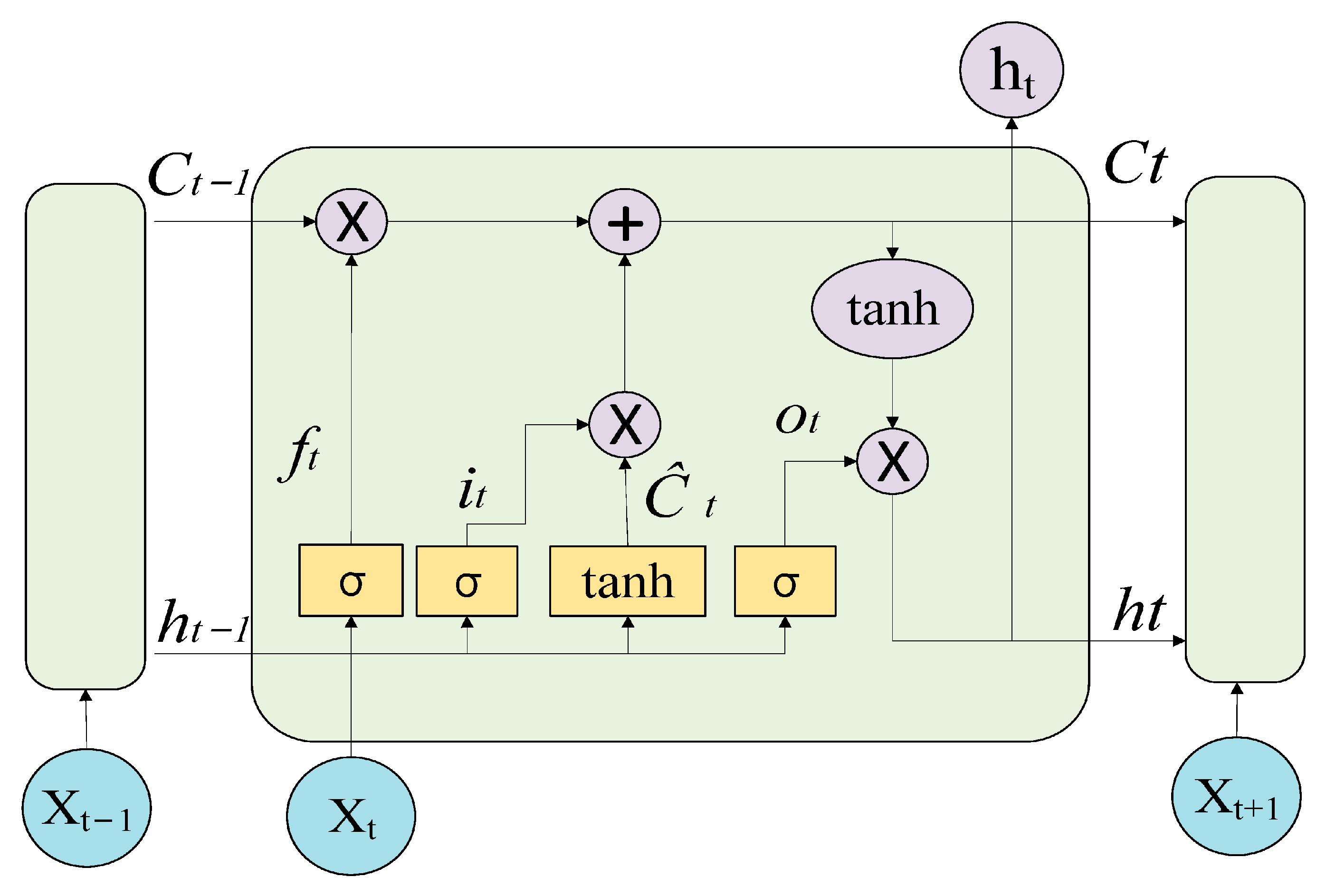
(1) LSTM effectively alleviates the gradient vanishing problem through three gate control mechanisms, the forget gate, input gate, and output gate, and can capture time dependencies ranging from tens of seconds to hundreds of seconds [29]. Figure 6 shows the LSTM model structure.
Figure 6.
LSTM unit structure.
The mathematical expressions for the input gate, forget gate, cell state update, cell state, output gate, and hidden state are shown in Equations (8)–(13).
where is the vector representation of the t-th time step of the input sequence, is the hidden state of the forward LSTM at the t-th time step, W is the weight matrix, b is the bias, σ is the sigmoid function, and ⊙ denotes element-wise multiplication.
In the input layer, multi-source drilling parameters (dynamic quantities such as pump pressure, riser pressure, inflow rate, and rotation speed, as well as static quantities such as well depth, borehole diameter, and mud density) are first concatenated with physical structural features to form a multi-dimensional time series window. This input is processed by a two-layer stacked LSTM network:
The output of the last layer of LSTM is mapped to a low-dimensional feature representation through a fully connected layer (FC1):
where is the temporal feature vector, is the hidden state at the last moment, is the bias vector of the fully connected layer, and is the weight matrix of the fully connected layer.
(2) CPO performance optimisation Grey Wolf Optimizer (GWO), Whale Optimisation Algorithm (WOA), Differential Evolution, and Sparrow Optimisation Algorithm (SSA) [30]. CPO is also widely used in hyperparameter optimisation for various models [31]. In the proposed LSTM–RF framework, model performance largely depends on the correlation of input features and the reasonable configuration of hyperparameters. High-dimensional feature spaces often contain redundant or noisy information, and inappropriate hyperparameters may lead to insufficient model stability and decreased generalisation ability [32]. To this end, this study introduces CPO to simultaneously achieve feature subset selection and hyperparameter optimisation.
Like other population-based meta-heuristic algorithms, CPO initiates the search process by initialising a set of individuals, as shown in Equation (16).
where n is the population size; represents the i-th candidate solution; and represent the upper and lower bounds of the search range; is a random number between [0, 1].
CPO mimics CP by using four different protection mechanisms—visual defence strategy, sound defence strategy, odour attack phase, and physical attack phase—to perform optimisation. The mathematical formulas are shown in Equations (17)–(20).
where is the optimal solution of function t; is the current individual position; is a random number based on a normal distribution; are random numbers between [0, 1], used to control the exploration range and direction; is the vector generated between the current CP and the random CP; is a random number between [1, N]; is a randomly generated binary vector of 0 and 1; is the parameter controlling the search direction; is the convergence speed factor; is the scaling factor; is the defence factor; is the odour diffusion factor; and is the gradient direction of the fitness function.
Let the output of the LSTM fully connected layer be , and the physically interpretable features (such as mud pit volume change rate, inlet and outlet flow difference, and riser pressure change) be . Then, the joint feature representation is shown in Equation (21).
In CPO, each candidate solution can be represented as , where is the feature selection mask used to determine which features are retained, and is the hyperparameter set. Through joint optimisation, the model can adaptively select the optimal feature combination and parameter configuration while ensuring physical plausibility.
Model hyperparameter optimisation mainly involves searching for hyperparameters for two submodels and time windows, i.e., optimising the three related parameters of LSTM, time window, and RF. The parameters optimised for LSTM are mainly the number of hidden units, the number of layers, and the dropout rate. The parameters optimised for the time window are mainly the length and stride. The parameters optimised for RF are mainly the number of trees, maximum depth, and feature ratio.
The fitness function for the CPO optimisation objective is defined as:
where F1 is the comprehensive performance index, FNR is the false negative rate, Delay is the warning delay, and , is the penalty coefficient. Through this design, the optimisation process can simultaneously improve recognition accuracy and early warning capabilities.
To mitigate the risk of overfitting and avoid redundant feature selection, this study introduced multiple constraint measures during the CPO optimisation process. First, feature sparsity constraints were set to limit the proportion of feature selection, thereby suppressing redundant information while ensuring the retention of key information. Second, a cross-well validation strategy was adopted to divide the training set and validation set between different wells to ensure the model’s generalisation ability under diverse geological conditions. Finally, to address the issue of relatively scarce well leakage samples, a category weight correction mechanism was introduced into the RF classifier to mitigate the impact of category imbalance on the model’s discriminative performance.
During real-time monitoring, sensor signals are often affected by short-term fluctuations, random noise, and instantaneous operational disturbances. If alarms are triggered solely based on the results of a single frame prediction, this can lead to a high false alarm rate, thereby undermining the reliability of the model in field applications. To address this issue, this study introduces an alarm confirmation frame count in the output layer. Based on the operational experience of field personnel, the alarm confirmation frame count is set to 15, with its calculation formula shown in Equation (23).
Among them, is the binary classification output of the model at time (1 = LC, 0 = normal), and is the number of alarm confirmation frames.
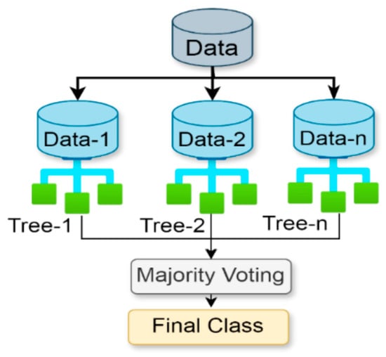
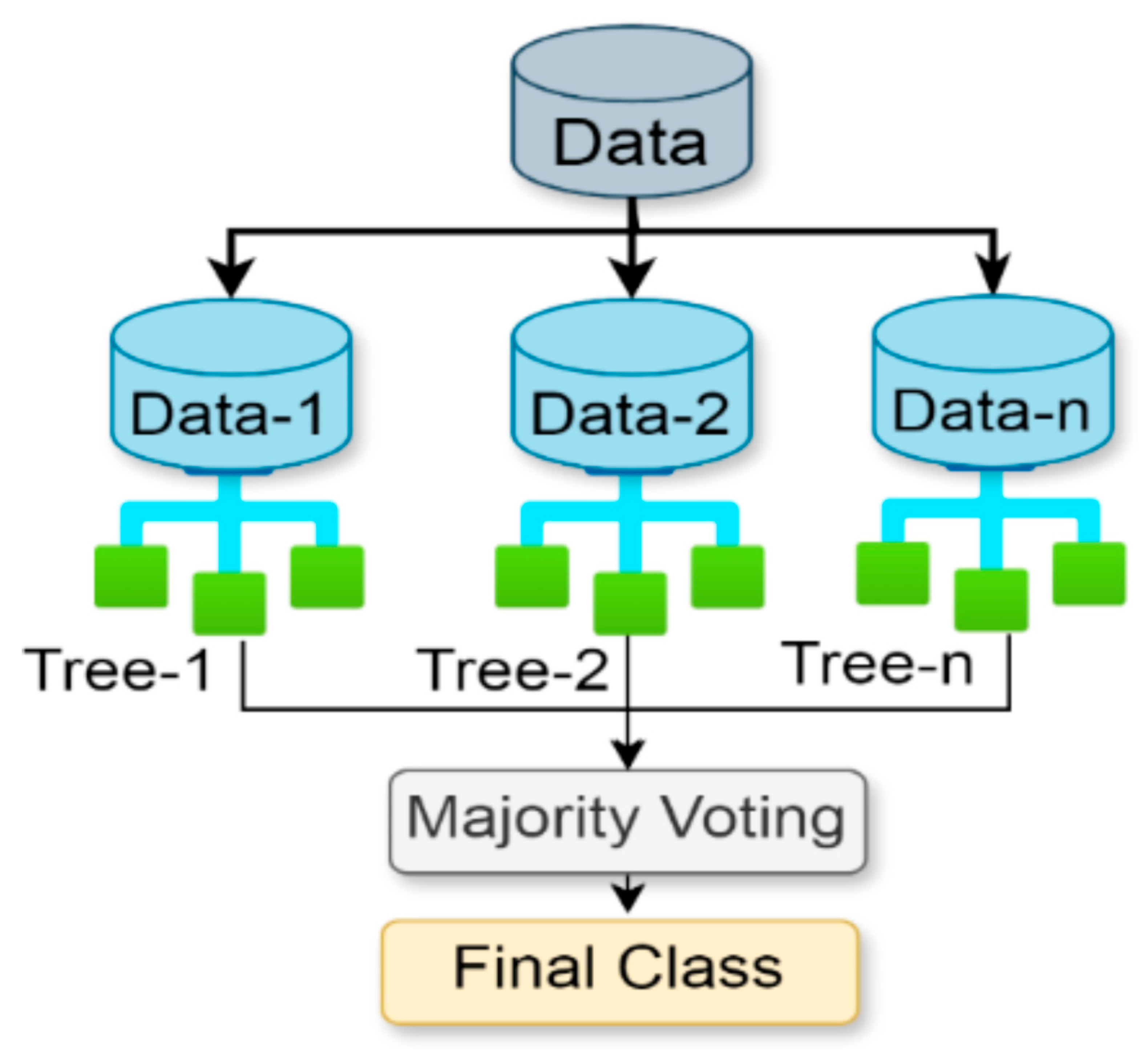
(3) RF is an ensemble learning method created to solve classification problems [33]. RF serves as the final classification module in the CPO–LSTM–RF framework, comprehensively discriminating between deep temporal features extracted by LSTM and physical structural features. RF is a bagging-type ensemble learning method that trains multiple decision trees and performs majority voting on their results, effectively overcoming the overfitting problem of a single classifier while maintaining high robustness in complex and noisy environments [34].
The basic idea behind RF is to use Bootstrap self-sampling to resample the training data, generating multiple different data subsets, and then build various decision trees based on these subsets [35]. Each tree introduces feature randomisation during training, i.e., only a subset of randomly selected features is considered when splitting nodes, thereby enhancing model diversity and reducing the correlation between trees. Finally, RF integrates the prediction results of each tree, as shown in Equation (24).
where represents the predicted category of the i-th tree, N is the number of trees, is the category with the most votes, and is the voting process.
The traditional LSTM–Softmax model performs only linear mapping and probability normalisation in the classification layer, resulting in a discriminative boundary that is approximately linear. This makes it difficult to handle the complex non-linear features of wellbore signals, particularly when dealing with sensor noise and outliers [36]. In contrast, RF can form complex non-linear decision boundaries through the hierarchical splitting of tree structures, better fitting the multi-dimensional feature patterns of wellbore evolution. Additionally, RF has strong robustness to outliers and is less likely to cause overall prediction errors due to individual outlier samples.
Another important advantage of RF is its feature importance assessment function. By calculating the Gini index or feature importance scores based on information gain, it is possible to quantify the contribution of different input features to the classification results.
where represents the Gini index at time t or in a certain state; is the proportion of k types of samples; k represents the total number of categories.
Each tree outputs predicted class for input . The final prediction of RF is determined by majority voting among the predictions of all trees.
where model refers to the most common class in all tree classifications.
This method not only reduces overfitting but also improves generalisation performance, making RF a powerful and reliable tool for classification tasks. Figure 7 illustrates the configuration of the RF classification model.
Figure 7.
Classification structure of RF.
3. Evaluation and Model Parameters
3.1. Evaluation and Experimental Environment
To compare the LC recognition performance of different models, two metrics, monitoring accuracy Acc and false negative rate FNR, are used to evaluate the models [37]. LC samples are treated as negative samples, and normal samples are treated as positive samples. The specific calculation equations are shown in Equations (27)–(30).
where True Positive (TP) indicates that LC occurred and was correctly predicted by the model, False Positive (FP) indicates that LC did not occur, but the model incorrectly predicted it as an LC event, False Negative (FN) indicates that LC occurred, but the model failed to predict it, classifying it as a non-LC event, True Negative (TN) indicates that LC did not occur and was correctly identified as a non-LC event by the model. Acc measures the overall correctness of the model by calculating the proportion of correctly classified samples (both LC and non-LC) to the total number of samples, Precision represents the proportion of correctly predicted LC events among all events predicted as LC, Recall indicates the proportion of actual LC events that were correctly predicted by the model, F1-score defined as the harmonic mean of Precision and Recall, it provides a balanced measure that considers both false alarms and missed detections. The confusion matrix is shown in Table 5.
Table 5.
True Result vs. Forecast Result.
The experimental environment employed Ubuntu 22.04 as the operating system, utilising Python 3.8 as the development language. To ensure efficient model training and experimentation, PyTorch version 2.7.1 was adopted, coupled with CUDA 12.8 to accelerate deep learning computations. Regarding the GPU, we used a GeForce RTX 5070 Ti (16 GB), which delivers robust parallel computing capabilities when processing large-scale datasets. Furthermore, the experimental setup was configured with 64 GB of RAM to ensure efficient operation during big data processing and complex computations.
3.2. Model Parameters
In the proposed CPO-LSTM-RF model, the hyperparameters of both LSTM and RF can be optimised. This paper employs a two-layer LSTM architecture, with model hyperparameters as shown in Table 6. For neural network parameter tuning, a combination of CPO and cross-validation was employed to explore different parameter combinations, thereby achieving optimal performance. In LSTM parameter tuning, the focus was on adjusting the learning rate, batch size, number of epochs, and dropout rate. For RF, parameter adjustments included n_estimators and max_depth to optimise model performance. Model parameters are shown in Table 7. To prevent model overfitting, this paper introduces early stopping as a method to mitigate this phenomenon.
Table 6.
Unoptimised model hyperparameters.
Table 7.
Optimised model hyperparameters.
4. LC Warning Model Experiment and On-Site Application
4.1. Comparison of CPO with Classical Optimization Algorithms
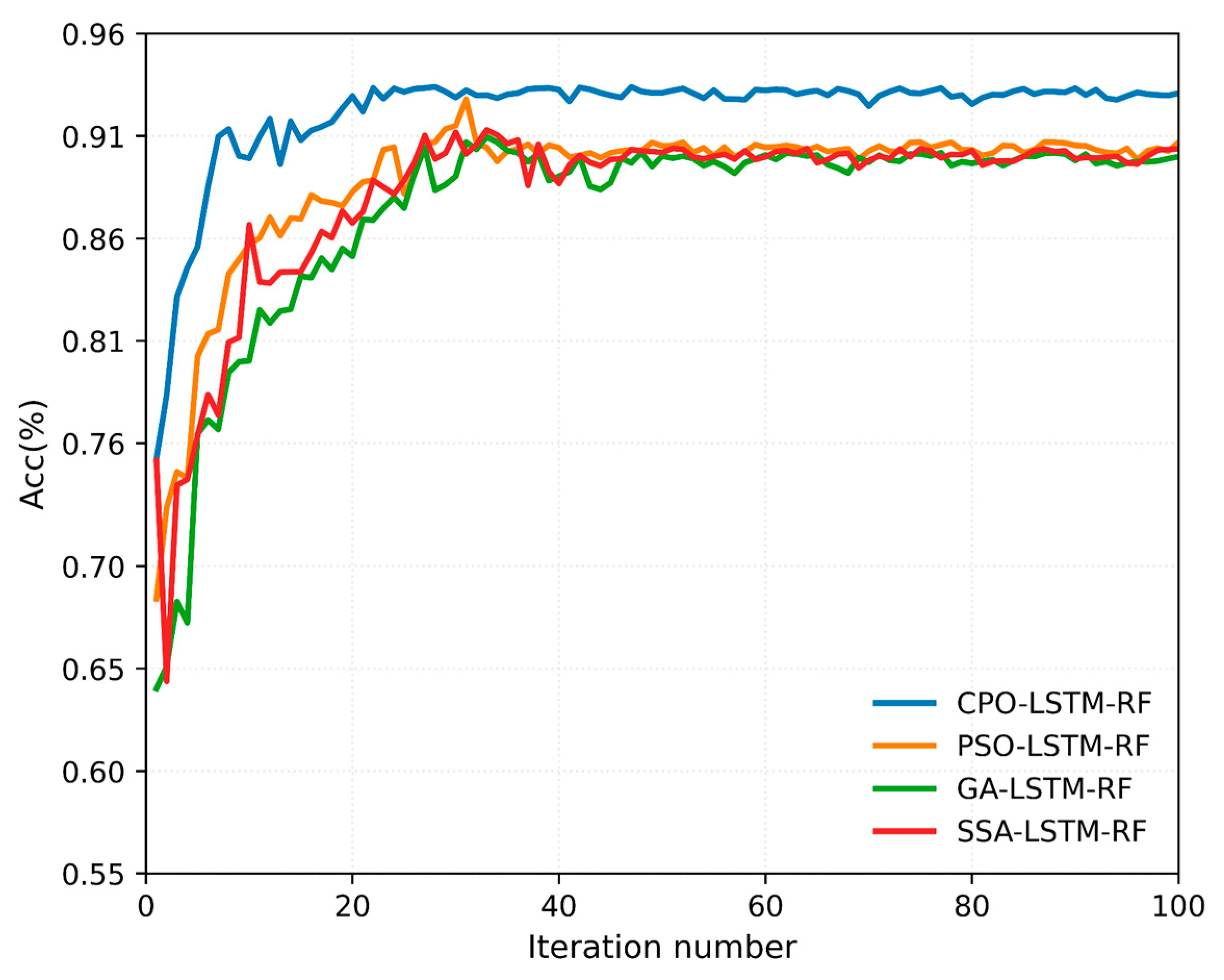
To validate the superiority of the CPO, experimental comparisons were conducted against classical optimization algorithms such as GA, PSO, and SSA. The parameters shown in Table 8 were employed throughout the experiments to ensure fairness in comparison and reliability of results.
Table 8.
Experimental parameter settings.
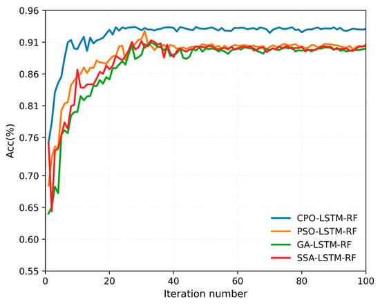
Figure 8 shows the fitness curves of four different models in the LC prediction task: CPO-LSTM-RF, LSTM-RF, LSTM, and RF. Experiments reveal that CPO-LSTM-RF achieves its optimal fitness value of 93.4% after only 22 iterations. In contrast, LSTM-RF, LSTM, and RF require 32, 46, and 42 iterations, respectively, to reach their optimal fitness values of 90.7%, 90.2%, and 90.4%. Thus, compared to other models, CPO-LSTM-RF can more rapidly and accurately identify the optimal input feature combinations and hyperparameter settings, achieving superior predictive performance.
Figure 8.
Changes in different optimization algorithms across iterations.
Among the various performance evaluation metrics for different models, as shown in Table 9, the CPO-LSTM-RF model achieved the highest accuracy (93.4%), precision (92.7%), recall (92.3%), and F1 score (92.5%). Table 9 highlights the significant advantage of the CPO-LSTM-RF model over the other three models in all evaluation metrics. These results demonstrate the effectiveness of CPO in optimizing LSTM-RF model parameters and emphasize the potential application of the CPO-LSTM-RF model for LC early warning.
Table 9.
Evaluation Metrics for Prediction Results of Four Optimization Algorithms.
4.2. Comparison Experiment of LC Warning
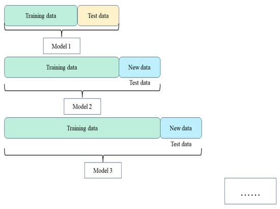
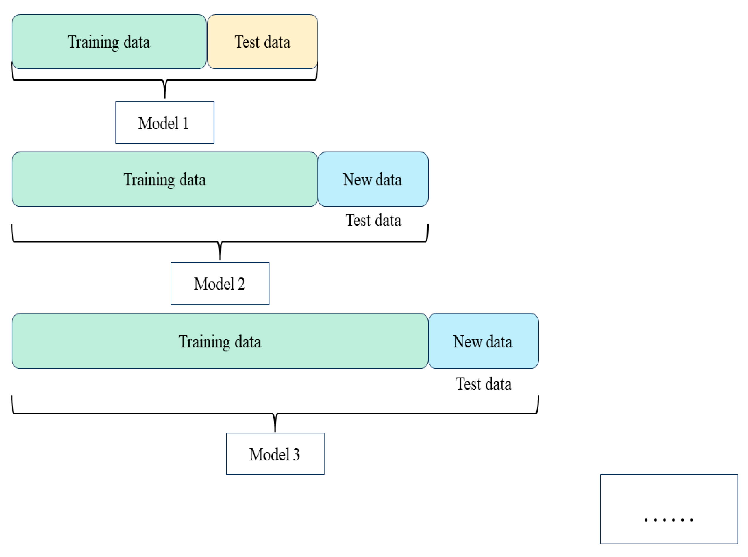
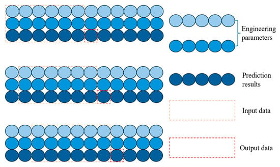
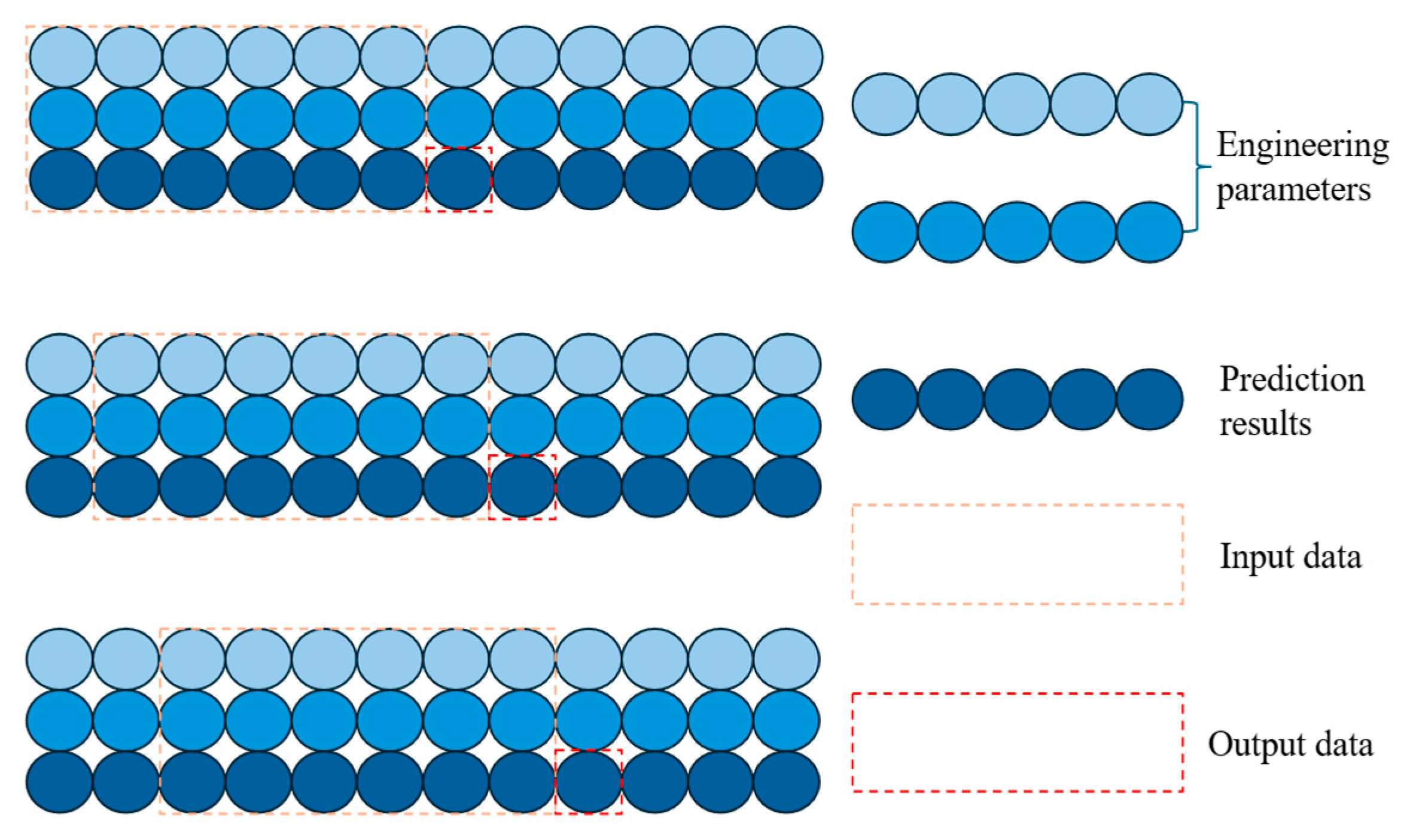
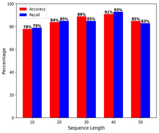
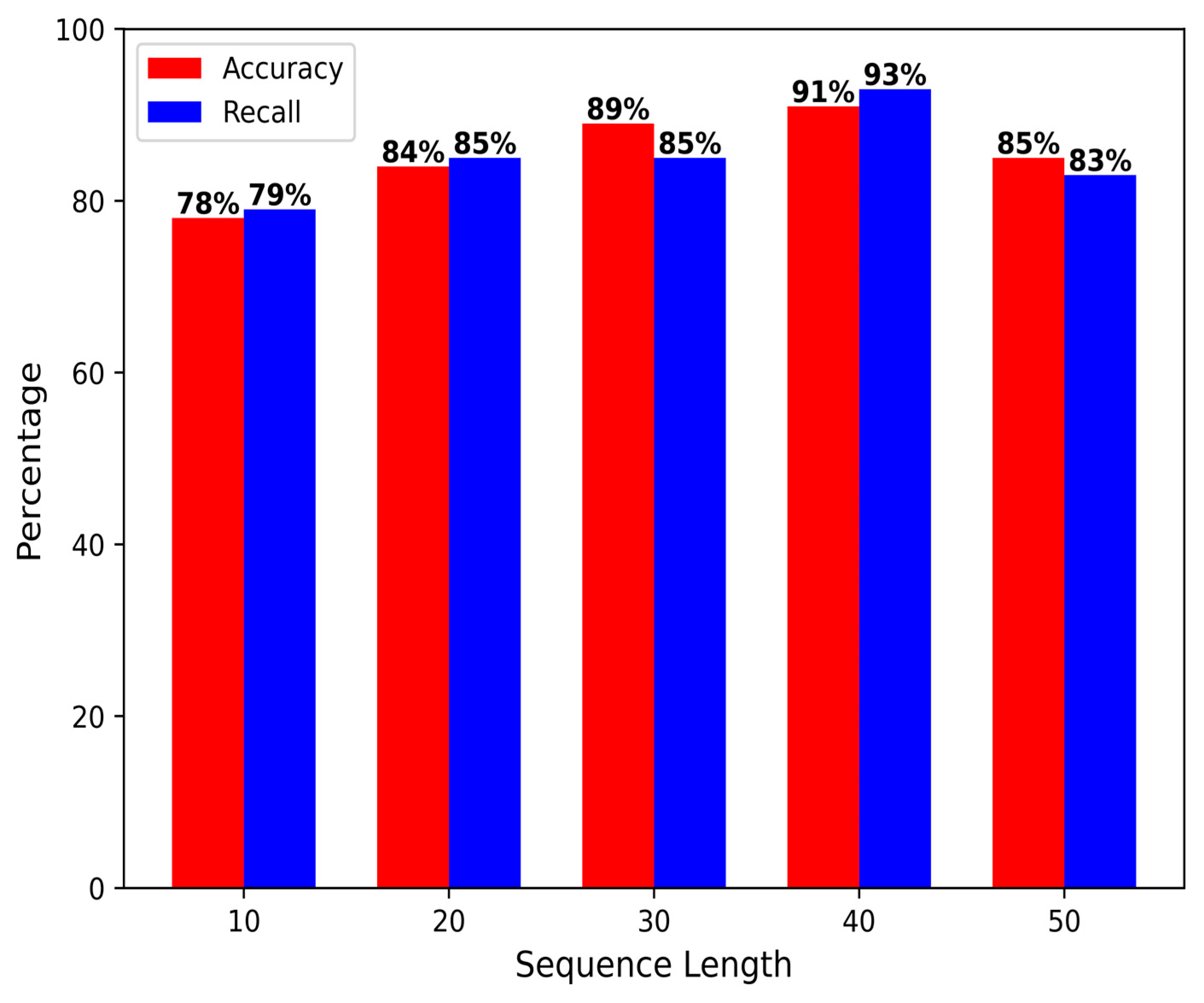
LSTM is a temporal forecasting model where the time step has a significant impact on model performance. The sliding window algorithm (Figure 9) constitutes a vital component of sequence prediction, an appropriate time step enhances robustness, preventing issues such as overfitting or underfitting. This study conducted comparative experiments across different time steps, with results presented in Figure 10. Analysis across five time steps (10, 20, 30, 40, and 50) revealed the model performed worst during testing at a time step of 10, achieving the lowest accuracy and recall rates of 78% and 79% respectively. Optimal performance was attained at a time step of 40, yielding an accuracy of 91% and a recall of 93%. Therefore, to ensure overall model performance and avoid false alarms and missed detections, a time step of 40 was selected for this study.
Figure 9.
Sliding window algorithm.
Figure 10.
Model Performance Comparison Across Different Time Steps.
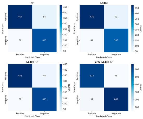
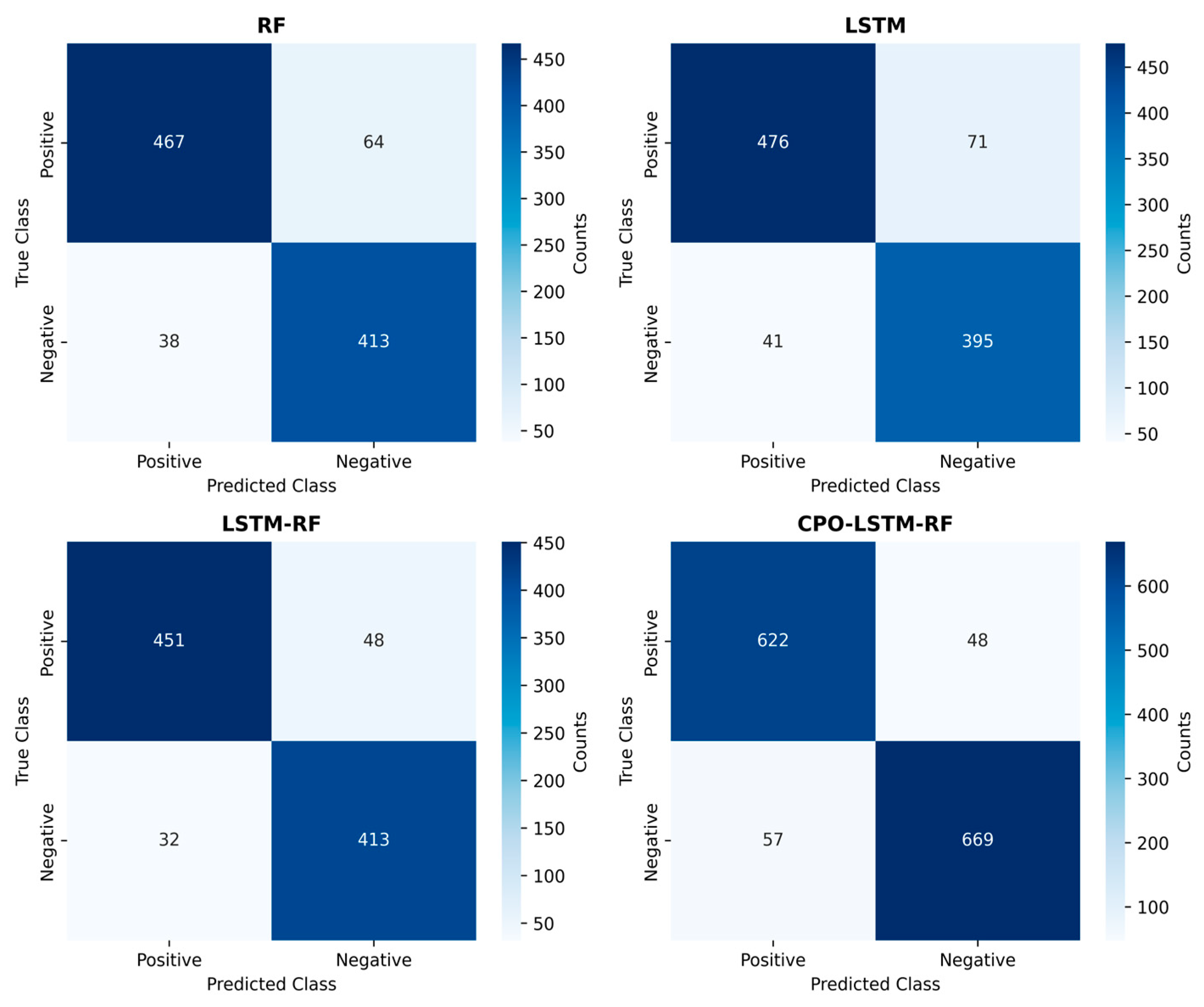
To further evaluate the performance of the CPO-LSTM-RF model, experimental comparisons were conducted between CPO-LSTM-RF and two classical long-range forecasting models: RF and LSTM. To assess the extent of performance improvement achieved by CPO over LSTM-RF, LSTM-RF was included as a comparison model. Consequently, this study employs RF, LSTM, and LSTM-RF as comparison models for CPO-LSTM-RF. The confusion matrices for different algorithmic models on the test set are presented in Figure 11.
Figure 11.
Confusion matrices for different models.
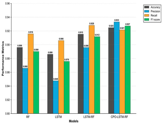
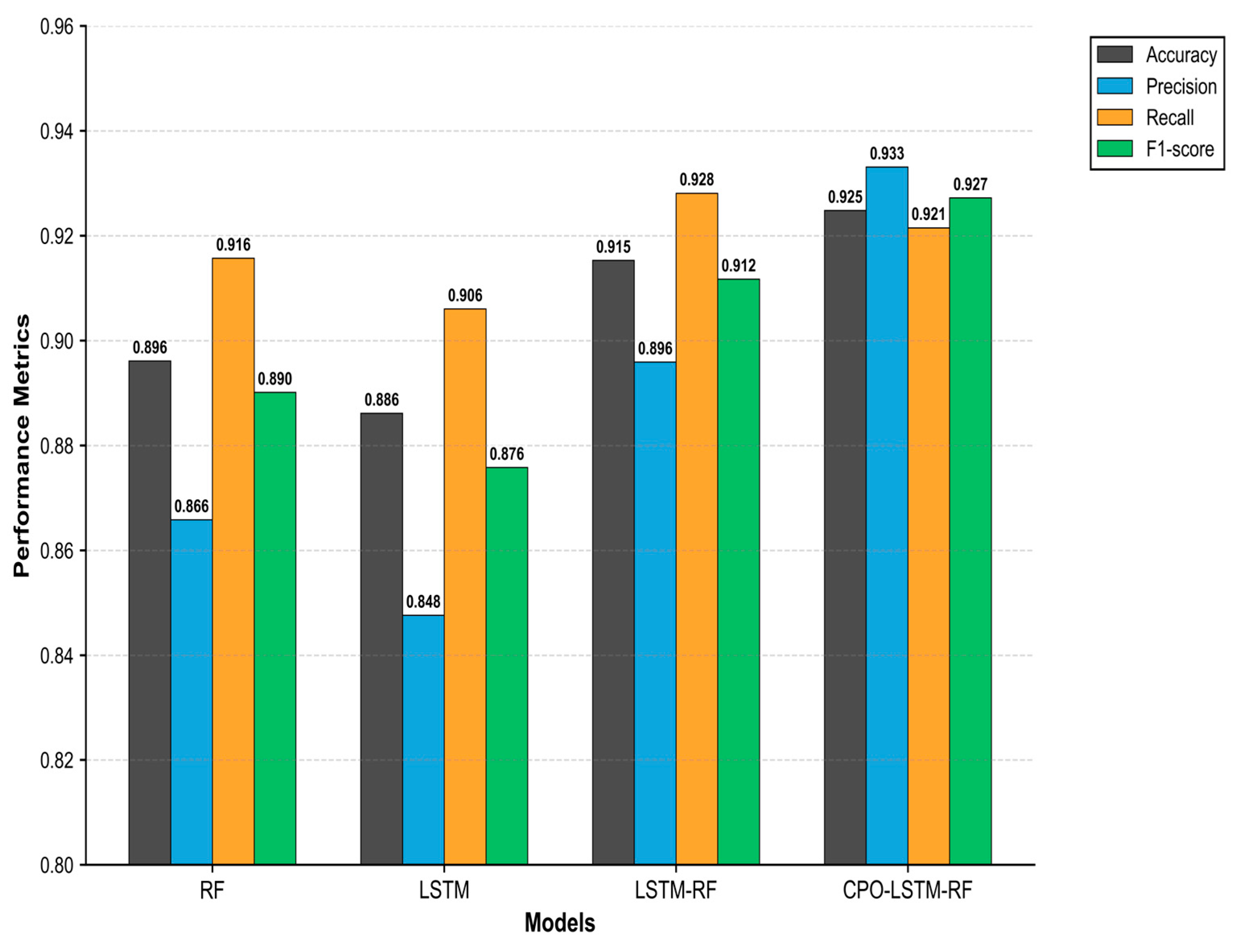
As shown in Figure 12, the CPO-LSTM-RF model achieved an evaluation metric of Accuracy 0.9248, Precision 0.9331, Recall 0.9215, and F1-score 0.9272, demonstrating superior performance compared to the other three models. The confusion matrix data indicates the performance ranking of the models as follows: CPO-LSTM-RF > LSTM-RF > RF > LSTM.
Figure 12.
Evaluation metrics for different models.
4.3. On-Site Application
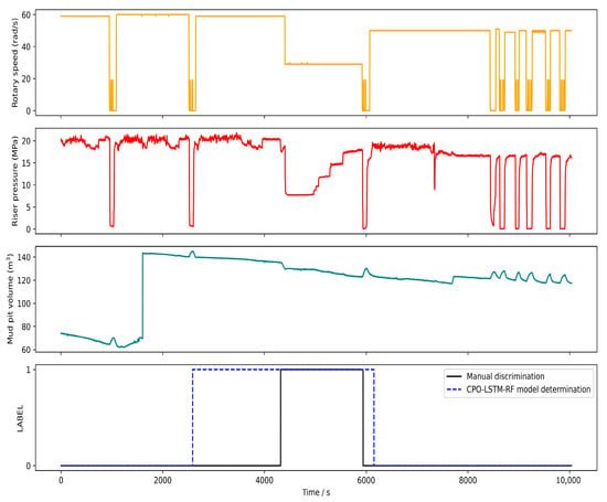
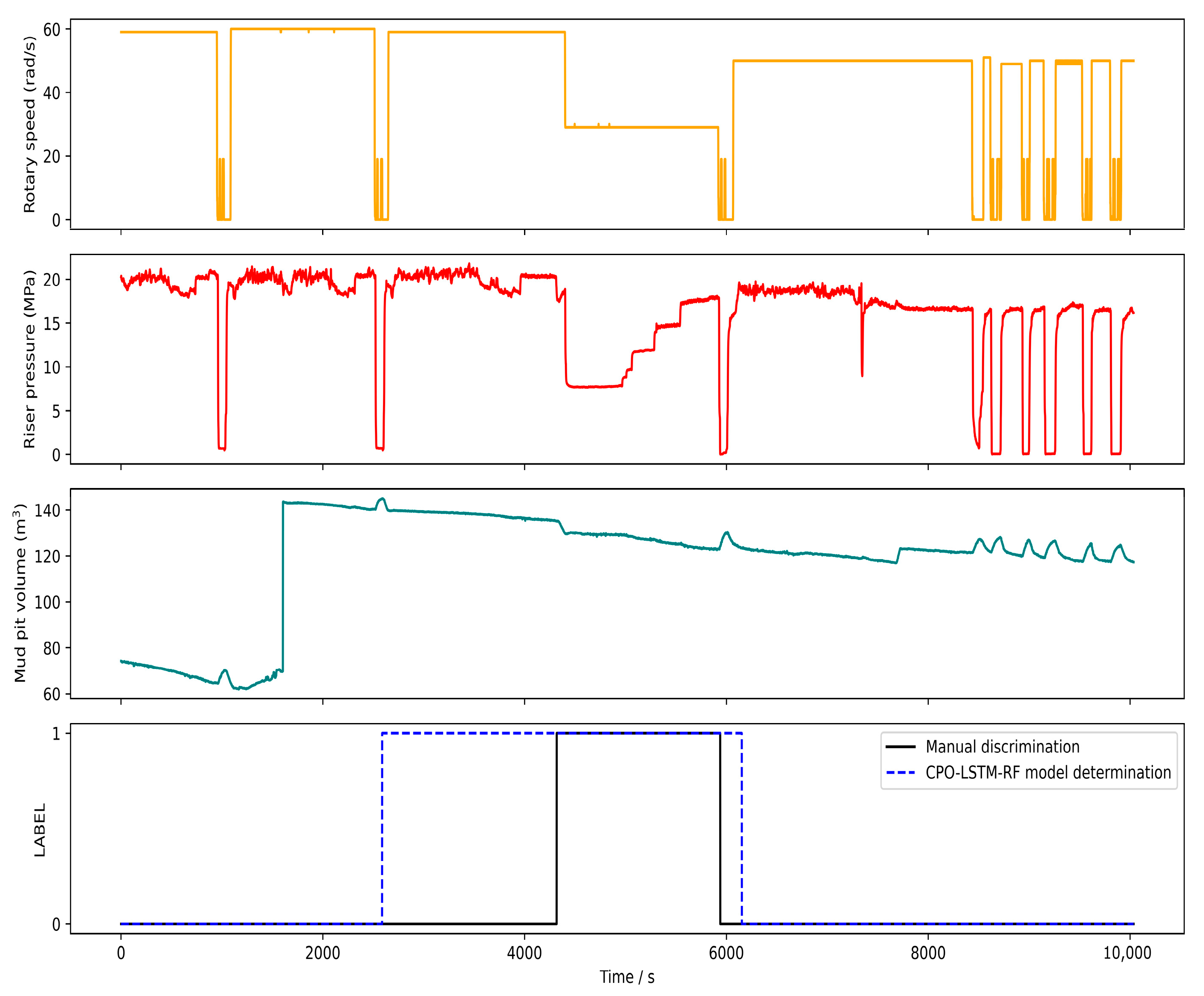
Analysis of representative flow loss cases from this oilfield provides intuitive evidence of the CPO-LSTM-RF model’s effectiveness in monitoring circulation loss. The comparison results between CPO-LSTM-RF and manual early warning are shown in Figure 13. The field construction report issued an LC alarm 5893 s after construction commenced, whereas the CPO-LSTM-RF model’s alarm time was significantly earlier than the construction report’s LC, occurring approximately 17 min ahead. This highlights the rationality and timeliness of the proposed model, which can provide a reference for field operators and substantially mitigate the likelihood of LC occurrence.
Figure 13.
Comparison of Model Classification and Manual Classification.
It should be clarified that this warning test was conducted offline via historical data verification rather than in real time. Whilst real-time alert systems are crucial in operational practice, the experimental data in this study primarily derive from historical records to validate the model’s warning accuracy and advance notice capability. In practice, once the model detects potential LC risks, field operators can promptly implement corresponding measures based on the alert information. These include adjusting drilling parameters and monitoring mud flow rates, thereby mitigating LC risks.
5. Conclusions
This paper proposes a wellbore leakage early warning method based on physical models and combinatorial neural networks, which has been validated using actual measurement data from X oilfield in the western Bohai Bay. The main conclusions are as follows:
- (1)
- The proposed physical constraint fusion framework demonstrates superior overall performance compared to the benchmark model, enabling more stable identification of LC risks while reducing both false positives and false negatives.
- (2)
- Incorporating physically interpretable features (mud pit volume variation, flow in/out differences, and riser pressure changes) significantly improved predictive stability.
- (3)
- CPO-LSTM-RF, when deployed in the field, provided warnings approximately 17 min earlier than those indicated in the report.
Overall, integrating physical constraints with optimised deep learning significantly enhances the accuracy, stability, and interpretability of LC early warning systems, demonstrating strong potential for field deployment.
Future work will involve cross-block data validation and refining real-time early warning and intervention recommendations for online deployment, thereby improving engineering applicability and generalisation capabilities.
Author Contributions
Conceptualization, F.H. and R.Q.; methodology, Y.S.; software, Y.S.; validation, Z.S.; data, J.Y.; writing—original draft preparation, Y.S. and R.Q.; writing—review and editing, J.L.; visualization, F.H.; supervision, J.Y. All authors have read and agreed to the published version of the manuscript.
Funding
This research is funded by the National Key Research and Development Program of China (No.2023YFC2813100).
Data Availability Statement
The original contributions presented in this study are included in the article. Further inquiries can be directed to the corresponding author.
Acknowledgments
The authors are very grateful for the support of the National Key Research and Development Program of China.
Conflicts of Interest
Authors Fangfei Huang, Zhibin Sha, Jingsong Lu and Rongrong Qi were employed by Guangzhou Marine Geological Survey (CGS), Guangzhou. The remaining authors declare that the research was conducted in the absence of any commercial or financial relationships that could be construed as potential conflicts of interest.
Abbreviation
The following abbreviations are used in this manuscript:
| LC | Lost Circulation |
| ML | machine learning |
| ANN | Artificial Neural Network |
| DL | Deep learning |
| SVM | support vector machine |
| BP networks | backpropagation neural networks |
| LSTM | long short-term memory neural networks |
| CNN | convolutional neural network |
| Attention | attention mechanism |
| CPO | Crested Porcupine Optimizer |
| RF | Random Forest |
| GWO | Grey Wolf Optimizer |
| WOA | Whale Optimisation Algorithm |
| SSA | Sparrow Optimization Algorithm |
| GA | Genetic Algorithm |
| PSO | Particle Swarm Algorithm |
| TP | True Positive |
| FP | False Positive |
| FN | False Negative |
| TN | True Negative |
References
- Azadivash, A. Lost circulation intensity characterization in drilling operations: Leveraging machine learning and well log data. Heliyon 2025, 11, e41059. [Google Scholar] [CrossRef] [Scilit]
- Amish, M.; Khodja, M. Review of detection, prediction and treatment of fluid loss events. Arab. J. Geosci. 2025, 18, 8. [Google Scholar] [CrossRef] [Scilit]
- Zhang, R.; Zhang, C.; Song, X.; Li, Z.; Su, Y.; Li, G.; Zhu, Z. Real-time prediction of logging parameters during the drilling process using an attention-based Seq2Seq model. Geoenergy Sci. Eng. 2024, 233, 212279. [Google Scholar] [CrossRef] [Scilit]
- Zhu, S.; Song, X.; Zhu, Z.; Yao, X.; Liu, M. Intelligent prediction of stuck pipe using combined data-driven and knowledge-driven model. Appl. Sci. 2022, 12, 5282. [Google Scholar] [CrossRef] [Scilit]
- Wu, S.; Zhang, L.; Fan, J.; Zheng, W.; Zhou, Y. Real-time risk analysis method for diagnosis and warning of offshore downhole drilling incident. J. Loss Prev. Process Ind. 2019, 62, 103933. [Google Scholar] [CrossRef] [Scilit]
- Miao, X.; Zhao, H.; Xiang, Z. Leakage detection in natural gas pipeline based on unsupervised learning and stress perception. Process Saf. Environ. Prot. 2023, 170, 76–88. [Google Scholar] [CrossRef] [Scilit]
- Zhang, K.; Gong, C.; Lu, H.; Ouyang, Y.; Xin, Q. Intelligent early warning model and intelligent reasoning method based on integrated learning for loss circulation. Oil Drill. Prod. Technol. 2023, 45, 47–54. [Google Scholar]
- Sun, Y.; Mao, L.; Liu, Q.; Zhao, P.; Zhu, H. Sand Screenout Early Warning Model Based on Combinatorial Neural Network. Rock Mech. Rock Eng. 2025, 1–24. [Google Scholar] [CrossRef] [Scilit]
- Moazzeni, A.; Nabaei, M.; Jegarluei, S.G. Prediction of lost circulation using virtual intelligence in one of Iranian oilfields. In Proceedings of the SPE Nigeria Annual International Conference and Exhibition, Tinapa-Calabar, Nigeria, 31 July–7 August 2010. SPE-136992-MS. [Google Scholar]
- Al-Hameedi, A.T.T.; Alkinani, H.H.; Dunn-Norman, S.; Flori, R.E.; Hilgedick, S.A. Real-time lost circulation estimation and mitigation. Egypt. J. Pet. 2018, 27, 1227–1234. [Google Scholar] [CrossRef] [Scilit]
- Abbas, A.K.; Bashikh, A.A.; Abbas, H.; Mohammed, H.Q. Intelligent decisions to stop or mitigate lost circulation based on machine learning. Energy 2019, 183, 1104–1113. [Google Scholar] [CrossRef] [Scilit]
- Sabah, M.; Mehrad, M.; Ashrafi, S.B.; Wood, D.A.; Fathi, S. Hybrid machine learning algorithms to enhance lost-circulation prediction and management in the Marun oil field. J. Pet. Sci. Eng. 2021, 198, 108125. [Google Scholar] [CrossRef] [Scilit]
- Aljubran, M.; Ramasamy, J.; Albassam, M.; Magana-Mora, A. Deep learning and time-series analysis for the early detection of lost circulation incidents during drilling operations. IEEE Access 2021, 9, 76833–76846. [Google Scholar] [CrossRef] [Scilit]
- Pang, H.; Meng, H.; Wang, H.; Fan, Y.; Nie, Z.; Jin, Y. Lost circulation prediction based on machine learning. J. Pet. Sci. Eng. 2022, 208, 109364. [Google Scholar] [CrossRef] [Scilit]
- Alsaihati, A.; Abughaban, M.; Elkatatny, S.; Shehri, D.A. Application of machine learning methods in modeling the loss of circulation rate while drilling operation. ACS Omega 2022, 7, 20696–20709. [Google Scholar] [CrossRef] [Scilit] [PubMed]
- Jafarizadeh, F.; Larki, B.; Kazemi, B.; Mehrad, M.; Rashidi, S.; Neycharan, J.G.; Gandomgoun, M.; Gandomgoun, M.H. A new robust predictive model for lost circulation rate using convolutional neural network: A case study from Marun Oilfield. Petroleum 2023, 9, 468–485. [Google Scholar] [CrossRef] [Scilit]
- Bin Irfan, M.W.; Busahmin, B. Rheological Characterization and Shale Inhibition Potential of Single-and Dual-Nanomaterial-Based Drilling Fluids for High-Pressure High-Temperature Wells. Processes 2025, 13, 1957. [Google Scholar] [CrossRef] [Scilit]
- Sun, Y.; Liu, Q.; Zhu, F.; Zhang, L. Sand Screenout Early Warning Models Based on Combinatorial Neural Network and Physical Models. Processes 2025, 13, 1018. [Google Scholar] [CrossRef] [Scilit]
- Zhu, Z.; Wan, M.; Sun, Y.; Gong, X.; Lei, B.; Tang, Z.; Mao, L. A Multi-Source Data-Driven Fracturing Pressure Prediction Model. Processes 2025, 13, 3434. [Google Scholar] [CrossRef] [Scilit]
- Zeng, F.; Du, X.; Guo, J.; Zhang, Y.; Chen, Z. Fracturing Pressure Prediction Model Based on Temporal and Spatial Feature Fusion in Hydraulic Fracturing. Rock Mech. Rock Eng. 2025, 58, 12715–12735. [Google Scholar] [CrossRef] [Scilit]
- Li, J.; Li, J.; Wang, C.; Verbeek, F.J.; Schultz, T.; Liu, H. MS2OD: Outlier detection using minimum spanning tree and medoid selection. Mach. Learn. Sci. Technol. 2024, 5, 015025. [Google Scholar] [CrossRef] [Scilit]
- Shi, L.-F.; Dai, Y.-F.; Yin, H.; Shi, Y. Pedestrian trajectory projection based on adaptive interpolation factor linear interpolation quaternion attitude estimation method. IEEE Trans. Instrum. Meas. 2025, 74, 9511009. [Google Scholar] [CrossRef] [Scilit]
- Khodarahmi, M.; Maihami, V. A review on Kalman filter models. Arch. Comput. Methods Eng. 2023, 30, 727–747. [Google Scholar] [CrossRef] [Scilit]
- Huang, L.; Qin, J.; Zhou, Y.; Zhu, F.; Liu, L.; Shao, L. Normalization techniques in training dnns: Methodology, analysis and application. IEEE Trans. Pattern Anal. Mach. Intell. 2023, 45, 10173–10196. [Google Scholar] [CrossRef] [Scilit]
- Lima, F.T.; Souza, V.M. A large comparison of normalization methods on time series. Big Data Res. 2023, 34, 100407. [Google Scholar] [CrossRef] [Scilit]
- Ashena, R.; Hekmatinia, A.-A.; Ghalambor, A.; Aadnoy, B.; Enget, C.; Rasouli, V. Improving drilling hydraulics estimations—A case study. J. Pet. Explor. Prod. Technol. 2021, 11, 2763–2776. [Google Scholar] [CrossRef] [Scilit]
- Zhou, D.; Zhou, C.; Zhang, Z.; Zhou, M.; Zhang, C.; Zhu, L.; Li, Q.; Wang, C. Intelligent Lost Circulation Monitoring Method Based on Data Augmentation and Temporal Models. Processes 2024, 12, 2184. [Google Scholar] [CrossRef] [Scilit]
- Zhang, S.; Samuel, R. Reducing False Alarms for Early Kick and Loss Detection (EKLD) in Real-Time Application Using Knowledge-Assisted Case-Based Reasoning. In Proceedings of the Abu Dhabi International Petroleum Exhibition and Conference, Abu Dhabi, United Arab Emirates, 4–7 November 2024; p. D011S029R001. [Google Scholar]
- Al-Selwi, S.M.; Hassan, M.F.; Abdulkadir, S.J.; Muneer, A.; Sumiea, E.H.; Alqushaibi, A.; Ragab, M.G. RNN-LSTM: From applications to modeling techniques and beyond—Systematic review. J. King Saud Univ.-Comput. Inf. Sci. 2024, 36, 102068. [Google Scholar] [CrossRef] [Scilit]
- Abdel-Basset, M.; Mohamed, R.; Abouhawwash, M. Crested Porcupine Optimizer: A new nature-inspired metaheuristic. Knowl.-Based Syst. 2024, 284, 111257. [Google Scholar] [CrossRef] [Scilit]
- Hua, Z.; Yang, Q.; Chen, J.; Lan, T.; Zhao, D.; Dou, M.; Liang, B. Degradation prediction of PEMFC based on BiTCN-BiGRU-ELM fusion prognostic method. Int. J. Hydrog. Energy 2024, 87, 361–372. [Google Scholar] [CrossRef] [Scilit]
- Yang, K.; Liu, L.; Wen, Y. The impact of Bayesian optimization on feature selection. Sci. Rep. 2024, 14, 3948. [Google Scholar] [CrossRef] [Scilit]
- Salman, H.A.; Kalakech, A.; Steiti, A. Random forest algorithm overview. Babylon. J. Mach. Learn. 2024, 2024, 69–79. [Google Scholar] [CrossRef] [Scilit]
- Khan, A.A.; Chaudhari, O.; Chandra, R. A review of ensemble learning and data augmentation models for class imbalanced problems: Combination, implementation and evaluation. Expert Syst. Appl. 2024, 244, 122778. [Google Scholar] [CrossRef] [Scilit]
- Garrido-Labrador, J.L.; Serrano-Mamolar, A.; Maudes-Raedo, J.; Rodríguez, J.J.; García-Osorio, C. Ensemble methods and semi-supervised learning for information fusion: A review and future research directions. Inf. Fusion 2024, 107, 102310. [Google Scholar] [CrossRef] [Scilit]
- Pearce, T.; Brintrup, A.; Zhu, J. Understanding softmax confidence and uncertainty. arXiv 2021, arXiv:2106.04972. [Google Scholar] [CrossRef] [Scilit]
- Mu, H.; Jiang, G.; Zhang, W.; Sun, J.; He, Y.; Dong, T.; Feng, Q.; Wang, Q.; Yang, L. Multidimensional Lost Circulation Risk Quantification Assessment Model Based on Ensemble Machine Learning. SPE J. 2025, 30, 2285–2295. [Google Scholar] [CrossRef] [Scilit]

Disclaimer/Publisher’s Note: The statements, opinions and data contained in all publications are solely those of the individual author(s) and contributor(s) and not of MDPI and/or the editor(s). MDPI and/or the editor(s) disclaim responsibility for any injury to people or property resulting from any ideas, methods, instructions or products referred to in the content. |
© 2026 by the authors. Licensee MDPI, Basel, Switzerland. This article is an open access article distributed under the terms and conditions of the Creative Commons Attribution (CC BY) license.