


Abstract
To address the challenges of poor data quality, reliance on manual intervention, and coarse evaluation granularity in the operation and maintenance of ultra-high-voltage (UHV) transformers, a condition assessment and decision-making model driven by a domain knowledge graph and multidimensional capability assessment is proposed. First, a collaborative data cleaning framework combining variational mode decomposition (VMD) and stacked denoising autoencoders (SDAEs) is established to reconstruct missing data and correct outliers while retaining signal features. Second, a domain knowledge graph for UHV transformers is constructed using a top-down approach. This graph structurally represents fragmented regulations, expert experience, and equipment ledgers, establishing a semantic network that connects condition parameters, components, and capabilities. Third, a multidimensional capability evaluation system is developed to map condition parameters to five core capabilities: insulation, load, short-circuit withstand, voltage regulation, and self-protection, providing more detailed condition information than a single overall score. Finally, a knowledge-driven diagnostic and decision-making model combines expert-assigned association values using a simplified fusion rule and uses graph relationships to link abnormal events with candidate failure modes and operation and maintenance recommendations. For 11 artificially corrupted samples, VMD–SDAE achieves a root mean square error (RMSE) of 0.1634 μL·L−1 and a mean absolute percentage error (MAPE) of 1.69% compared with 0.3319 μL·L−1 and 3.38% for standalone SDAE. Additional comparisons, ablation experiments, and sensitivity analyses examine the cleaning performance and its limitations. A case study produces condition assessment results consistent with on-site judgments and provides maintenance recommendations with traceable reasoning paths.
1. Introduction
Due to the geographical mismatch between energy resources and load centers in China, constructing a long-distance, high-capacity, low-loss ultra-high-voltage (UHV) transmission network has become a key measure for addressing cross-regional energy allocation and ensuring national energy security [1,2]. With progress toward the “dual carbon” (peak carbon emissions and carbon neutrality) targets and the development of a new power system, the scale of the UHV grid continues to expand. As core hubs within this network, UHV transformers directly affect the safety and stability of the large-scale power grid. However, UHV transformers are structurally complex and costly to manufacture, and they operate over the long term in environments characterized by intense electromagnetic interference and complex meteorological conditions. Even a single failure can therefore result in significant economic losses and social repercussions. Consequently, research on accurate condition assessment and evidence-based maintenance decision-making is of great significance.
The widespread adoption of smart sensing and Internet of Things (IoT) technologies has led to the accumulation of vast amounts of online monitoring data and unstructured text from transformer operation and maintenance. However, existing condition assessment and decision-making systems still face significant challenges in three key areas: data cleaning, condition assessment, and maintenance decision-making.
- (1)
- Data cleaning: Previous studies have proposed data cleaning methods based on statistics [3,4], isolation forests [5,6], and deep learning [7,8,9]. However, online monitoring data from UHV substations are often affected by environmental noise and transmission interference and may contain outliers, missing values, and non-stationary noise. Directly using such low-quality data for evaluation can distort feature extraction, leading to misclassification or missed detection. A key challenge therefore remains—suppressing noise while preserving the subtle features of equipment state evolution when processing strongly coupled, nonlinear, multi-source, and heterogeneous data from UHV transformers.
- (2)
- Condition assessment: The power industry has accumulated extensive domain knowledge, including dispersed regulations and guidelines (e.g., DL/T 1685 [10] and DL/T 1723 [11]) and expert experience. Existing studies have attempted to incorporate this knowledge by simplifying it into static thresholds or simple tree-like hierarchies [12,13,14]. However, this fragmented knowledge management model underutilizes domain knowledge and lacks deep semantic reasoning. It overlooks the complex couplings among condition parameters and between these parameters and equipment capabilities, resulting in coarse-grained evaluation results that struggle to support complex fault attribution and decision-making reasoning.
- (3)
- Maintenance decision-making: Traditional assessment and maintenance methods largely rely on manual table lookups and subjective scoring and lack an integrated process that spans from “data perception” through “knowledge inference” to “decision execution” [15,16,17]. Knowledge graph applications have been reported in healthcare [18], fault diagnosis [19], relay-protection defect knowledge extraction [20], aviation assembly fault diagnosis [21], and power-system fault diagnosis and disposal [22]. However, deep reasoning models that integrate multidimensional capability assessment with knowledge graphs specifically for UHV transformers remain in their infancy. Consequently, discontinuity persists between condition assessment and maintenance decision-making.
Existing KG-based studies in power equipment can be grouped into three categories. The first is the knowledge-organization route, in which KGs are built from defect records, relay-protection defects, or equipment ledgers to support entity–relation extraction and knowledge retrieval [20]. These studies improve knowledge access, but their nodes mainly represent equipment/defect entities; condition parameters are not systematically mapped to multiple capabilities, and the graph is not used as an assessment rule base. The second is the fault-handling route, in which KGs for distribution network fault dispatch and case recommendation support fault disposal using graph matching [23]. Such graphs are event- and case-centered rather than capability-centered, and they do not perform five-dimensional condition scoring. The third is the diagnosis/portrait route, in which KGs are combined with MLP, GCN, or joint reasoning for transformer state profiling or fault diagnosis [24,25,26]. These studies improve fault identification, but most remain component- or fault-centered, rely on static thresholds or tree-like hierarchies, and often stop at fault type or location. They rarely link condition parameters → five capabilities → failure mode → O&M measure. In contrast, the KG in this work explicitly contains components, condition parameters, assessment criteria, five capabilities, failure modes, and corrective measures. It is used not only for retrieval but also as the rule repository for two-layer assessment of state quantities and capabilities and as the causal structure for Bayesian-inspired fault attribution and O&M decision-making.
For Bayesian diagnosis, existing studies can be grouped into classical naive Bayes, improved naive Bayes/WRSR [27], and partially observable Markov/decision models [28]. Classical naive Bayes requires conditional independence and conditional likelihoods; improved naive Bayes/WRSR still depends on sufficient fault samples or relatively complete probabilistic parameters; partially observable models require state-transition and observation models. For UHV transformers, historical fault samples are scarce, and full conditional probability tables are difficult to estimate. The proposed model therefore does not estimate full CPTs. Instead, it uses KG-defined causal relations and expert-confidence indices as prior domain knowledge and adopts a simplified fusion rule to combine expert-assigned values when multiple abnormal events occur. This is intentionally a simplified engineering inference model, not a statistically calibrated Bayesian network; its advantages are transparency and applicability under data scarcity. The methodological novelty therefore lies in the integration of data cleaning, five-capability assessment, KG-based fault attribution, and differentiated O&M decision-making, rather than the isolated use of VMD–SDAE, a KG, or Bayesian inference.
To address these limitations, a method is proposed for evaluating the condition of ultra-high-voltage transformers and making decisions based on a domain-specific knowledge graph. The purpose of this method is to address the challenges of poor data quality and underutilized knowledge in existing systems by establishing a dual-driven assessment and decision-making process based on “data knowledge” to support equipment condition evaluation and maintenance planning. The main innovations and contributions of this paper include:
- (1)
- A VMD–SDAE Collaborative Data Cleaning Framework: VMD decomposition and SDAE reconstruction are combined to repair monitoring-data contamination. Comparative, ablation, corruption, parameter-sensitivity, and KDE-quantile experiments examine the component contributions and identify the conditions under which the workflow improves recovery.
- (2)
- A Domain Knowledge Graph for UHV Transformers: To tackle the underutilization of fragmented domain knowledge, this work transforms scattered regulations, expert experience, and equipment ledgers into a structured semantic network using a top-down ontology construction method. Unlike existing KGs that mainly support defect retrieval or fault dispatch [19,20,22,23], the proposed KG explicitly links components, condition parameters, assessment criteria, five capabilities, failure modes, and corrective measures, and serves as both an assessment rule repository and a reasoning structure.
- (3)
- An Integrated Assessment and Decision-Making Model: To bridge the gap between condition assessment and maintenance decision-making, this model establishes an integrated process from anomaly detection to candidate fault attribution and strategy generation. Unlike KG-based diagnosis studies that stop at fault identification [24,25,26] or Bayesian/decision models that require relatively complete likelihoods or transition/observation models [27,28], this model uses the KG as a causal structure and expert-assigned confidence values as prior domain knowledge and integrates five-capability assessment with simplified Bayesian inference to produce interpretable, differentiated O&M strategies with traceable reasoning paths.
The remainder of the article is organized as follows. Section 2 describes the data cleaning method, the domain knowledge graph construction method, the multidimensional capability assessment framework, the condition assessment, and decision-making model. In Section 3, the data cleaning, evaluation, and decision-making results are provided. Finally, the conclusions are given in Section 4.
2. Methods
2.1. A Collaborative Data Cleaning Method Based on VMD–SDAE
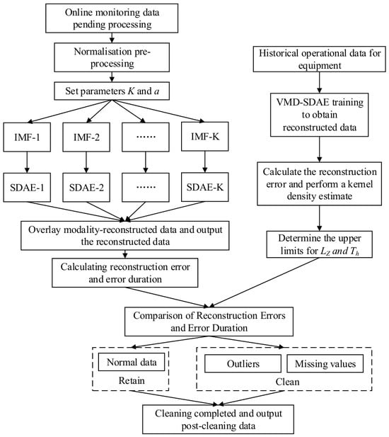
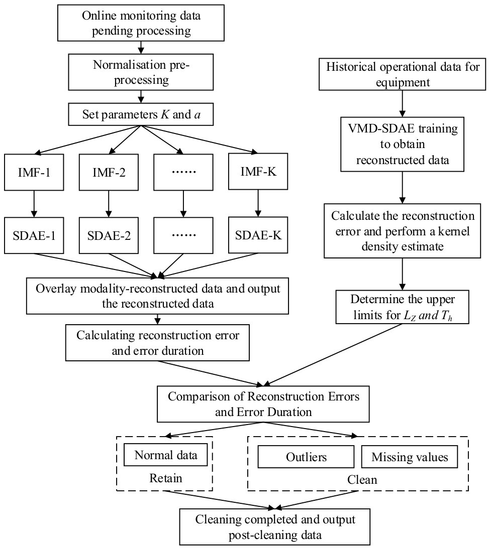
To address the complex coupling of non-stationary noise and meaningful features in the online monitoring data of UHV transformers, this paper proposes a two-stage data cleaning framework that combines variational mode decomposition (VMD) with a stacked denoising autoencoder (SDAE), as illustrated in Figure 1. The core concept of this framework is to first use VMD to decompose the complex raw signal into multiple intrinsic mode functions (IMFs) with distinct center frequencies, thereby achieving a preliminary separation of noise and signal at different scales. Subsequently, independent SDAE models are trained for each IMF component based on its specific characteristics to perform precise denoising and reconstruction. Finally, the reconstructed results of each component are aggregated to obtain high-quality, cleaned data.
Figure 1.
VMD–SDAE collaborative data cleaning framework.
VMD adaptively decomposes the original signal f(t) into multiple IMFs with distinct central frequencies by solving a constrained variational problem. Its core lies in finding the center frequency and bandwidth of each mode such that the sum of all modes can reconstruct the original signal. Directly solving a constrained variational problem is computationally challenging; therefore, it is transformed into an unconstrained optimization problem that is easier to handle. The algorithm introduces a quadratic penalty term and Lagrange multipliers:
where K is the predefined total number of decomposition modes; uk(t) is the k-th IMF; ωk represents the center frequency of the k-th mode; δ(t) is the Dirac delta function; j is the imaginary unit; f(t) is the given input signal, which is the online monitoring data of the UHV transformer to be decomposed; α is the quadratic penalty factor used to balance data fidelity and modal bandwidth constraints; and λ(t) is the Lagrange multiplier function.
Denoising autoencoders incorporate a data corruption mechanism into the conventional autoencoder architecture, enabling them to extract more robust features. However, when dealing with the complex nonlinear evolution patterns of UHV transformers, the feature representation capabilities of this shallow network architecture remain limited. By stacking multiple layers of denoising autoencoders, data features can be extracted hierarchically. For each IMF component uk(t) obtained from the VMD decomposition, this paper constructs and trains an independent SDAE network. Historical data from the equipment’s normal operating state are used as the training set, enabling each SDAE model to learn the normal feature distribution of its corresponding IMF component.
The VMD mode number is chosen using a decomposition quality criterion that combines modal separation and the distribution of center-frequency spacings. For modes ordered by center frequency, O(K) is the mean normalized spectral overlap between adjacent modes. U(K) is the mean absolute deviation of the normalized adjacent center-frequency spacings from the uniform spacing 1/(K − 1). The composite criterion uses equal weights:
A smaller composite score is preferred together with a coefficient of variation R below 0.5, where R is the sample standard deviation of adjacent center-frequency spacings divided by their mean.
During the data cleaning phase, the test data undergo the same VMD decomposition and are then input into the corresponding SDAE model for reconstruction. The final reconstructed signal is obtained by summing the individual reconstructed components. Anomalies are identified by calculating the reconstruction error between the original and reconstructed data. The upper limits for reconstruction error and error duration are determined by analyzing the reconstruction error of the trained model using kernel density estimation (KDE). The decision rules are as follows:
- (1)
- If the reconstruction error for a data point exceeds the upper limit and the duration of the error does not exceed the upper limit, that point may be an outlier caused by a device malfunction or interference.
- (2)
- If the reconstruction error for a data point exceeds the threshold, the duration of the error exceeds the upper limit, and the value remains at 0 or a fixed value for an extended period, that point may be a missing value caused by a temporary sensor failure or a communication port malfunction.
- (3)
- If neither the reconstruction error nor the duration of the error for a data point exceeds the upper limit, that point is considered to represent data from a normal operating state.
- (4)
- If the reconstruction error for a data point exceeds the upper limit and the duration of the error exceeds the upper limit, but the data exhibit a continuous variation trend and does not remain at 0 or a fixed value for an extended period, that point is identified as abnormal operational data reflecting the true state of the equipment. The original value is retained with an anomaly flag, rather than being replaced by the reconstructed value.
For data points identified as missing or contaminated outliers, the original values are replaced with the SDAE reconstructions to correct data quality anomalies.
2.2. Building a Knowledge Graph in the Field of Ultra-High-Voltage Transformers
The knowledge graph constructed in this study for UHV transformer condition assessment and decision-making is a domain-specific knowledge graph. By integrating multi-source data—including assessment and O&M guidelines—and extracting knowledge from expert experience, a knowledge base for UHV transformer condition assessment and decision-making was established. This knowledge base subsequently served as the foundation for constructing the domain knowledge graph. Three main approaches to knowledge graph construction exist: top-down, bottom-up, and hybrid. Given that UHV transformer condition assessment is characterized by highly specialized domain knowledge, intricate logical rules, and stringent accuracy requirements, the top-down approach is adopted in this work. This approach first designs the schema layer and then extracts instances from heterogeneous data sources.
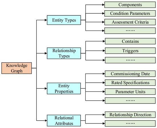
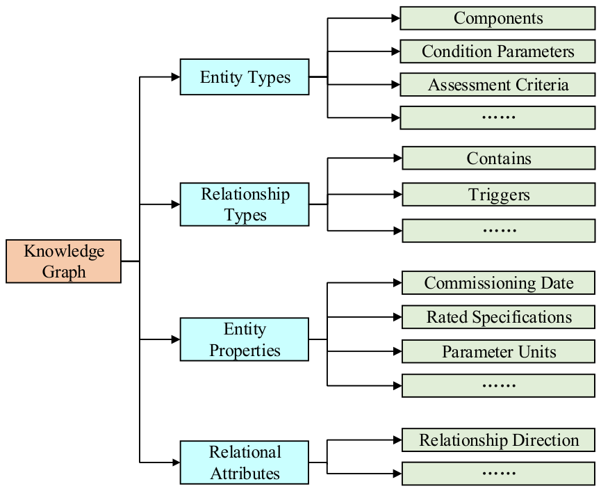
The schema layer defines the structural specifications of the knowledge; it does not store concrete facts but instead specifies the types of knowledge that the graph can accommodate. To achieve a structured representation of knowledge pertaining to UHV transformer condition assessment, this paper designs the domain ontology illustrated in Figure 2 as the schema layer. This ontology delineates four core entity types, namely, components, condition parameters, assessment criteria, and corrective measures, thereby constituting the semantic framework of the knowledge graph.
Figure 2.
Schema layer structure.
Following the schema design, knowledge identification, screening, structuring, and fusion were performed manually. The source knowledge comprised assessment and maintenance guidelines, including DL/T 1685-2017 and DL/T 1723-2017, together with documents and experience-based criteria supplied by domain experts. The graph builder reviewed these materials to identify equipment components, condition parameters, assessment conditions, and corresponding measures, and organized the selected knowledge into entity records and subject–predicate–object relationships consistent with the schema. Knowledge from the different sources was manually aligned and consolidated during this process.
The structured knowledge was organized in spreadsheet tables and exported as CSV files. Entity records contain a unique identifier, a name, a category, and a graph label; selected tables additionally contain a ‘belong to’ attribute indicating the associated component or condition parameter. Relationship records contain the start-node identifier, end-node identifier, and the relationship type. The CSV files were loaded into Neo4j using the neo4j-admin import command, with separate node files and a relationship file. Cypher queries were subsequently used to retrieve and visualize the resulting graph and relevant subgraphs.
Domain experts provided the source materials and practical assessment criteria, which were manually organized into entities and relationships. The resulting graph has not yet undergone independent expert review. The graph stores typed semantic relationships without numerical edge weights. Relationships specify, for example, which assessment criterion applies to a condition parameter and which condition grade or deduction is associated with that criterion. The deduction values belong to the assessment rules and are represented by linked score nodes; they are not weights assigned to graph edges.
To quantify the scale of the constructed domain knowledge graph, its core elements are statistically summarized as follows. The knowledge graph encompasses 287 entities, including 15 equipment and component entities and 58 condition parameter entities. The relationship table contains 695 semantic relationship records in subject–predicate–object form. These records associate the entities through typed relations, including assessment basis, assessment grade, deduction, test type, component membership, and corrective measure, thereby forming a structured knowledge base for the subsequent condition assessment and decision-making model.
2.3. Multidimensional Capability Assessment Based on Operational Status
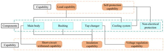
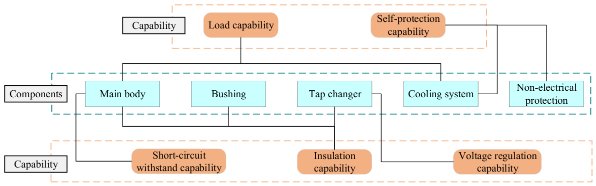
Ultra-high-voltage transformers incorporate a variety of functionally distinct, technologically sophisticated components, which can be categorized into five major groups from both functional and structural perspectives: the main body, bushings, tap changers, the cooling system, and non-electrical protection systems. Drawing on the equipment’s functional characteristics and expert experience, the operational status of UHV transformers is classified into five dimensions: insulation capability, short-circuit withstand capability, voltage regulation capability, load capability, and self-protection capability. An integrated analysis of these five capabilities is conducted, establishing correlations between them and the principal components of UHV transformers. The relationships between components and capabilities in the operational status of UHV transformers are illustrated in Figure 3.
Figure 3.
Diagram showing the relationship between the operational status and capabilities of ultra-high-voltage transformers and their components.
In the evaluation system built on this framework, the operational status of UHV transformers occupies the highest level; it represents both the overall operational performance of the equipment and the ultimate objective of the evaluation. The operational status of UHV transformers encompasses five capabilities—insulation, load, short-circuit withstand, voltage regulation, and self-protection. Therefore, the performance layer is positioned below the objective layer, and the indicator layer, constituting the third and lowest level, contains the various condition parameters that reflect these capabilities.
2.4. A Model for Evaluating Operational Status Based on a Domain Knowledge Graph
2.4.1. Model Architecture
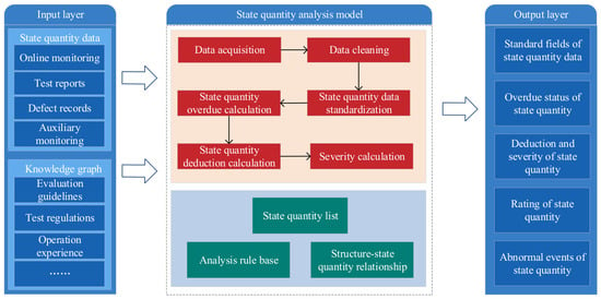
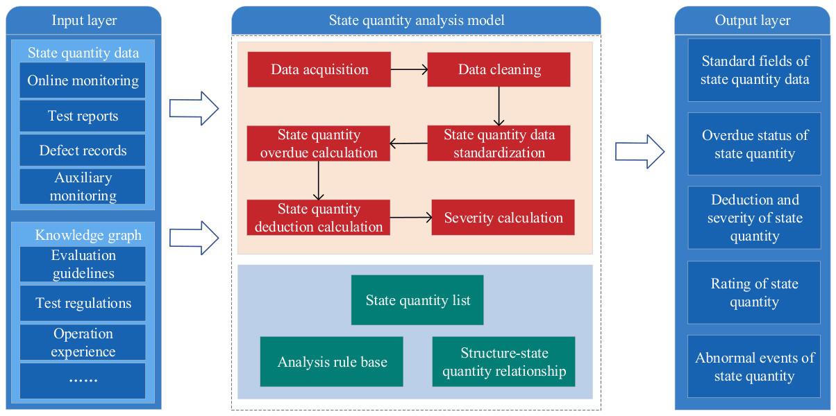
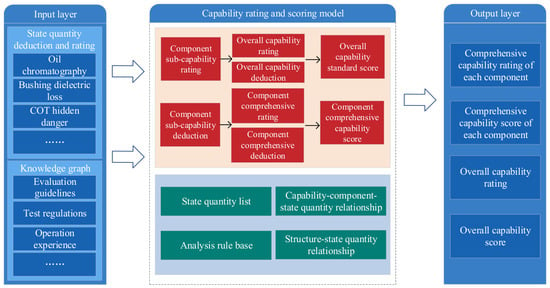
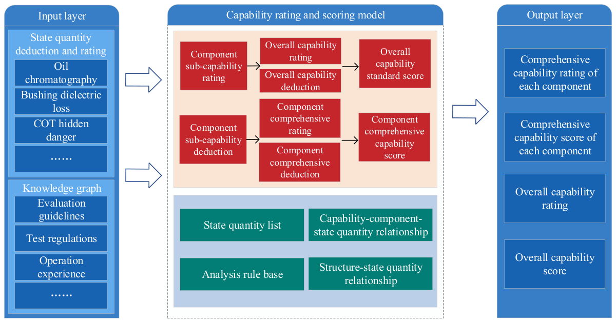
As the data processing foundation of the entire evaluation system, the state-quantity analysis model is responsible for collecting multi-source, heterogeneous data from online monitoring, test reports, and defect records and performing data cleaning, standardization, and quantification. Using the component–condition parameter relationships and predefined assessment rules in the knowledge graph, the model evaluates the input condition data and assigns condition grades and deduction values. The state-quantity analysis model integrated with the knowledge graph is shown in Figure 4. Building upon the state-quantity analysis model, the capability rating and scoring model is presented in Figure 5.
Figure 4.
State-quantity analysis model.
Figure 5.
Capability rating and scoring model.
2.4.2. Construction Method
The assessment criteria were compiled manually from the applicable assessment and maintenance guidelines and the documents and experience-based criteria supplied by experts. Each criterion associates a condition parameter with an explicit assessment condition, a condition grade, and a deduction value. Four condition grades are used: normal, caution, abnormal, and severe. Thresholds and deductions are predefined knowledge entries rather than parameters learned from the monitoring data. The knowledge graph organizes these entries and their associations, while the assessment model compares the input condition data with the relevant conditions and applies the corresponding grading and deduction rules.
The implementation steps for the operational condition evaluation model are as follows:
- (1)
- From a functional and structural perspective, ultra-high-voltage transformers are classified into five major components: the main body, bushings, tap changers, the cooling system, and non-electrical protection systems. Correspondences are established among the system as a whole, its components, capabilities, and condition metrics. Using the raw condition metric data and the knowledge graph as model inputs, the condition metric analysis model performs rating and penalty calculations for each condition metric. The evaluation results for each condition parameter, combined with the deduction algorithms provided by the analysis rule library in the knowledge graph, are then used to rate and deduct points for the capabilities of the five major components.
- (2)
- The capability rating results of the five major components serve as a prerequisite for evaluating the equipment’s overall capability. A cascading rating is performed at the component capability level by leveraging the capability–component–condition metric relationships in the knowledge graph, thereby rating all capabilities of all components. The equipment’s overall capability rating across the five dimensions follows the “shortest-stave” principle, with the lowest rating among the corresponding capabilities of each component determining the equipment’s overall capability rating.
- (3)
- The five-dimensional capability deduction for the equipment as a whole is computed as the sum of the capability deductions across all components. These totals are then converted to a score for the equipment’s overall capability based on the score ranges specified in the capability rating standards.
2.5. Knowledge-Driven Bayesian Diagnostic Decision Model
2.5.1. Knowledge Graph-Based Bayesian Inference Algorithm
Bayesian inference, grounded in probability and statistical theory, motivates the use of observed abnormal events to assess candidate failure modes. Bayes’ theorem provides the general probabilistic relationship expressed in Equation (3).
where D represents the feature set and Ci represents the class.
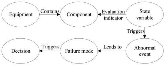
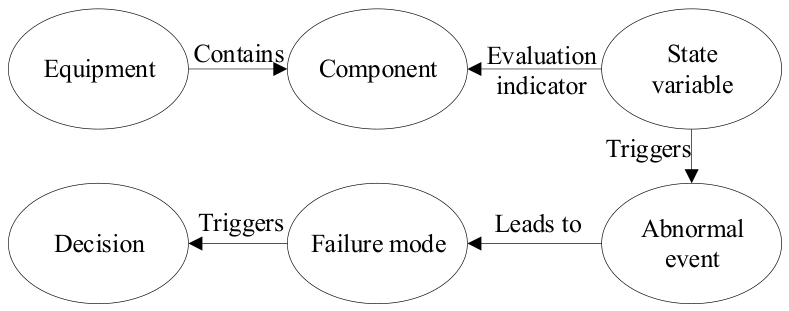
A knowledge graph in the UHV transformer domain can provide structured prior knowledge to support Bayesian inference. Figure 6 illustrates the ontology structure and the relationships between entities relevant to fault diagnosis and decision-making.
Figure 6.
Schematic diagram of the ontology structure and relationships between entities in the diagnosis and decision-making knowledge graph.
Naive Bayes is a simplified inference method derived from Bayes’ theorem. Assuming that the categories are fixed and all features are conditionally independent given the class, the conditional joint probability can be decomposed as shown in Equation (4):
Combining (3) and (4) yields the core formula for naive Bayes:
Using Bayesian diagnostic reasoning as a conceptual starting point, this study combines expert-assigned single-event values using a simplified multi-event fusion rule. Equation (6) is used as an engineering approximation for accumulating support for candidate faults. It is not derived directly from Equations (3)–(5) or from independence among abnormal events alone, and its output is not established as a calibrated posterior fault probability.
The calculation method is shown in Equation (6):
For a given candidate failure mode A, qᵢ denotes the expert-assigned value associated with the i-th active abnormal event, and Sᵢ denotes the diagnostic support obtained by combining the first i active events. The same calculation is performed separately for each candidate failure mode. The resulting scores summarize the event-based support for the candidate failure modes and are not interpreted as statistically calibrated fault probabilities. The diagnostic results, together with the condition assessment results, knowledge graph relationships, and predefined scenario-triggering rules, provide the basis for retrieving relevant O&M recommendations.
The three expressions in Equation (6) correspond to one, two, and three abnormal events, respectively. The same combination rule is applied successively when further events are present. For input values in [0, 1], the rule keeps the combined support within [0, 1]. The subtraction term limits the increment as support increases; it does not estimate or correct statistical dependence between evidence items.
The expert-assigned values constitute prior domain knowledge and are distinct from the prior fault probability in Bayes’ theorem; no equivalence to a uniform prior distribution is assumed. The fusion rule does not explicitly model statistical dependence among abnormal events. Correlated or repeated evidence may therefore overstate the combined support, and the diagnostic output should be interpreted with reference to the physical relationships among the observed abnormalities.
2.5.2. Fault Diagnosis Framework
The fault diagnosis framework is designed to map the outputs of the condition assessment model to specific fault modes. This process involves the following steps:
- (1)
- Based on industry standards and expert experience, construct a detailed knowledge graph of equipment fault modes and corresponding abnormal events, where fault modes are classified into two categories:
- •
- Category I Faults: Internal faults within the core or bushing, such as arc discharge, partial discharge, and overheating;
- •
- Category II Faults: Functional faults, such as insulation aging, moisture ingress, tap changer defects, and cooling system failures.
- (2)
- When a condition parameter exceeds a defined threshold, the condition assessment model outputs an abnormal event. Drawing on Bayesian diagnostic reasoning, these events are treated as observational evidence for candidate failure modes. When multiple events support the same failure mode, Equation (6) is used to combine their expert-assigned values.
- (3)
- A separate association index system is established for events across different dimensions. The single-event values are provided by domain experts on the basis of equipment fault mechanisms and operation and maintenance experience, and are stored in the knowledge graph as prior domain knowledge. For a given fault mode, the values are restricted to [0, 1]. The values for primary events are at least 0.5, those for secondary events are at most 0.4, and those for unrelated events are set to 0. The expert-assigned single-event values used in the case study are reported in Section 3.2. These values provide inputs to Equation (6), rather than representing multi-event fusion results.
- (4)
- Relevance between an event and a failure mode is determined based on the membership index. If the membership is positive, the event is deemed relevant; otherwise, it is considered irrelevant, and failure modes unrelated to the event are excluded from the output.
2.5.3. Operation and Maintenance Decision-Making Framework
The equipment operation, maintenance, and repair decision-making model is designed to establish response measures for ultra-high-voltage transformers. It covers five typical scenarios in daily management: routine maintenance, anomaly detection, fault diagnosis, capability enhancement, and risk control. Drawing on relevant maintenance guidelines and reference response measures for transformers at other voltage levels, this model organizes decision-making measures and scenarios to construct an operation, maintenance, and repair decision-making system. The specific process is as follows:
- (1)
- Identify key decision-making factors and summarize decision-making scenarios. Classification standards are established, and decisions are categorized according to seven common types of O&M measures, forming an O&M decision-making knowledge base stored as graph nodes and relationships.
- (2)
- Extract the core factors influencing O&M strategies and identify representative decision-making scenarios. Based on actual operating conditions, typical scenarios that can trigger maintenance decisions are summarized, and an association graph linking scenarios to measures is constructed.
- (3)
- Based on the O&M decision-making knowledge base, trigger conditions and implementation guidelines are designed item by item for each typical scenario, thereby constructing the O&M decision-making model.
- (4)
- Following the execution of approved O&M measures, newly acquired condition data can be used as input to the state-quantity analysis model for reassessment. This provides a basis for comparing equipment conditions before and after maintenance. The use of maintenance outcomes to update assessment rules and diagnostic parameters remains a direction for future work.
The generated O&M measures are intended to support engineering decision-making rather than replace professional judgment. In practical applications, recommendations involving conflicting diagnostic evidence, uncertain data quality, or high-impact maintenance actions should be subject to expert review. In particular, outage arrangements, major maintenance operations, and changes to operating modes require confirmation using established O&M approval procedures before execution.
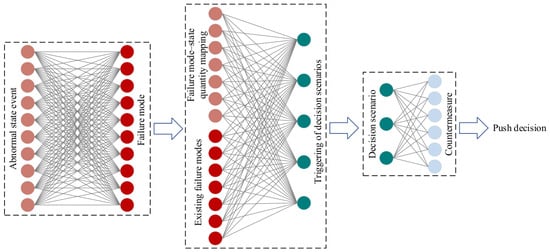
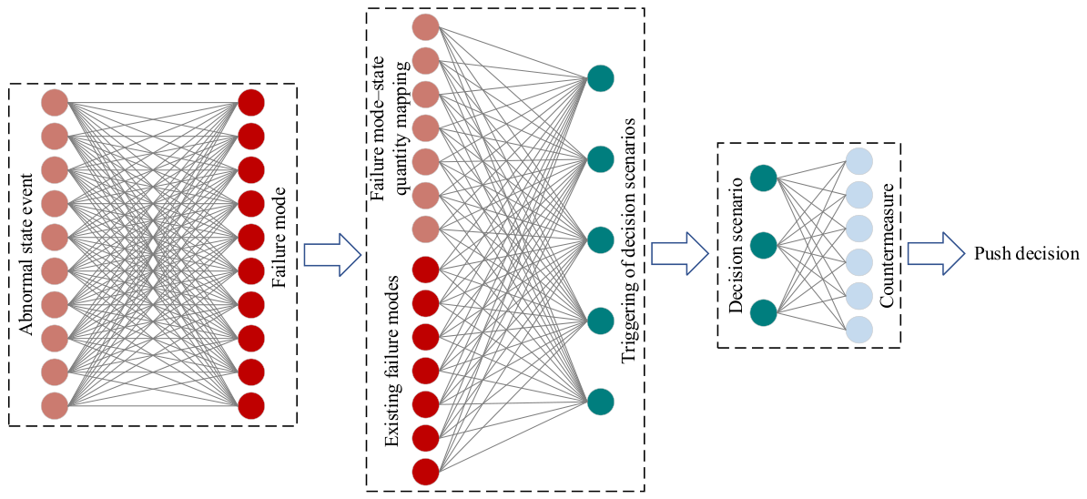
Figure 7 shows the functional diagram of the fault diagnosis and O&M decision-making model. Common O&M measures include the following seven categories: emergency O&M response, manual patrols, online monitoring, live-line testing, de-energized testing, de-energized maintenance, and live-line maintenance.
Figure 7.
Functional diagram of the fault diagnosis and O&M decision-making model.
3. Results
3.1. Validation and Analysis of Data Cleaning Results
3.1.1. Experimental Setup and Evaluation Metrics
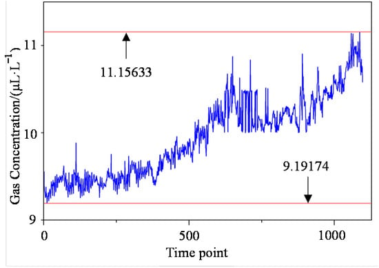
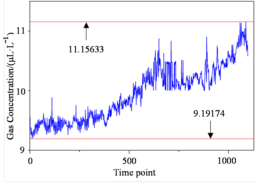
Hydrogen monitoring data were collected from a UHV transformer between January 2024 and January 2026 at a sampling interval of 4 h. Data from January 2024 to July 2025 were used for training, and data from August 2025 to January 2026 were used for testing. Figure 8 presents the test sequence. The reference sequence before artificial contamination provided the target for evaluating cleaning accuracy.
Figure 8.
Test data. The two red horizontal lines mark the upper bound (maximum value, 11.15633 μL·L−1) and the lower bound (minimum value, 9.19174 μL·L−1) of the test dataset.
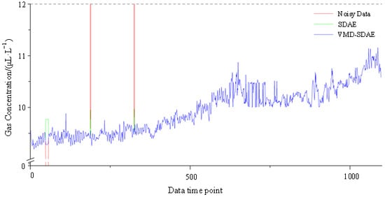
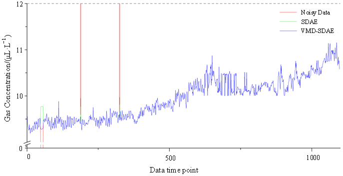
The number of VMD modes, K, was set to 4, and the balance parameter was set to 3000. The SDAE input layer consisted of 90 nodes, with three hidden layers containing 60, 40, and 60 nodes, respectively. The number of training epochs was set to 1000, and the bias was initialized to 0. The initial connection weights were randomly generated between 0 and 0.01, while the learning rates for both the weights and biases were set to 0.1. Additionally, 10% random noise was added to the input data. A normal data distribution model was then obtained with training on the training dataset. Subsequently, kernel density estimation was applied. With a confidence level of 0.98, the reconstruction error threshold for the normal state was determined to be 0.277474, and the maximum tolerance duration was set to 6. Artificial missing values were introduced at time points 48–56, and outliers were injected at time points 188 and 325, yielding a test dataset containing controlled anomalies. The cleaning results of the VMD–SDAE method were then compared with those of the standalone SDAE model. Figure 9 presents a comparison of the cleaned data.
Figure 9.
Comparison of results from the two cleaning methods.
In the figures, the red curves denote the original noisy data, the green curves represent the SDAE-cleaned results, and the blue curves correspond to the VMD–SDAE-cleaned results. In the normal data regions, both methods produce results that closely follow the original data, thereby preserving the undisturbed signal. Simultaneously, both methods successfully reconstructed the zero-valued missing data and corrected outliers that deviated substantially from the normal range. As shown in the figure, when handling continuous missing values, the reconstruction curve of the standalone SDAE model tends to flatten. This behavior can be attributed to the fact that SDAE, as a global feature-learning method, tends to output the mean or principal components of the training data when imputing missing sequences, thereby compromising the local high-frequency fluctuation characteristics of the signal. In contrast, the proposed VMD–SDAE method, leveraging the VMD preprocessing step, can isolate modal components containing high-frequency details and perform targeted reconstruction. Consequently, its reconstruction results not only accurately fill data gaps but also more effectively preserve the non-stationary fluctuation details of the original signal, closely tracking the variation trends of the actual data. The specific numerical comparisons are summarized in Table 1.
Table 1.
Comparison of cleaned values with original values using the two methods.
To systematically and objectively evaluate the integrated solution proposed in this paper that combines data cleaning, domain knowledge graphs, and intelligent evaluation and decision-making, the RMSE and MAPE metrics were employed to quantify the effectiveness of the VMD–SDAE data cleaning method.
- (1)
- Root Mean Square ErrorHere, N represents the number of samples in the specified evaluation set; xi and zi are the original and reconstructed values, respectively, corresponding to time step i.
- (2)
- Average Absolute Percentage Error
As shown in Table 1, based on the anomaly correction results, the VMD–SDAE cleaned values are closer to the original data. The RMSE and MAPE of the VMD–SDAE method were 0.1634 μL·L−1 and 1.69%, respectively, whereas those of the SDAE method were 0.3319 μL·L−1 and 3.38%, indicating considerably larger errors. These comparative experiments demonstrate that the VMD–SDAE method outperforms the standalone SDAE in both preserving data characteristics and correcting outliers. The metrics reported here were calculated over the 11 points described above to illustrate the ability of VMD–SDAE to repair corrupted samples (N = 11). In the subsequent experiments, full-sequence metrics use N = 1097, whereas corrupted sample metrics, where reported, use N = 11. These illustrative results and the subsequent method comparison results are reported separately and are not pooled.
For evaluation, a sample is considered uncorrupted if the absolute difference between its input and reference values does not exceed 10−12. It is counted as a modified uncorrupted sample if the absolute difference between its final output and input values exceeds 10−12. This tolerance distinguishes numerical equality from an actual modification. The resulting count measures preservation of the samples unaffected by artificial contamination.
3.1.2. Ablation Study
Three variants were constructed to examine the contributions of decomposition, neural reconstruction, and denoising pretraining. SDAE removes only VMD while retaining detrending and the matching training and detection rules. VMD-only removes only SDAE: the same VMD components are summed directly, and KDE is calibrated using this variant’s own training reconstruction errors. No interpolation is introduced. This variant tests removal of the neural reconstruction stage within the present workflow and is not a separately optimized VMD denoising method. VMD–SAE removes only the noise added during pretraining, while retaining the random number calls, network architecture, and remaining training procedure.
Table 2 summarizes the ablation results. The complete VMD–SDAE model achieved an RMSE of 0.017296 μL·L−1 compared with 0.018178 μL·L−1 for SDAE without VMD, representing a relative reduction of approximately 4.85%. Their MAPE values were 0.017875% and 0.018741%, respectively, and neither variant modified an uncorrupted sample under the defined tolerance. Removing SDAE increased RMSE to 1.012748 μL·L−1 and modified 79 uncorrupted samples, showing that direct summation of the VMD components does not replace the reconstruction stage in this workflow.
Table 2.
Ablation results for the baseline contamination case. RMSE is evaluated over the complete test sequence; MAPE is reported as a percentage. Modified uncorrupted samples are counted using the 10−12 tolerance defined in Section 3.1.1.
VMD–SAE yielded an RMSE of 0.017326 μL·L−1, which is close to the complete model’s result. Thus, the baseline ablation provides only limited evidence of an incremental benefit from denoising pretraining.
3.1.3. Comparison with Conventional and Hybrid Methods
To complement the component ablation experiments, VMD–SDAE was compared with median filtering, wavelet denoising, CEEMDAN–SDAE, and adaptive Kalman filtering followed by Rauch–Tung–Striebel smoothing (AKF–RTS). CEEMDAN–SDAE combines complete ensemble empirical mode decomposition with adaptive noise and SDAE reconstruction, providing a decomposition–network comparison model. All methods were evaluated using the same 1097-sample input sequence containing the same 11 corrupted samples. RMSE and MAPE were calculated over both the complete sequence and the corrupted samples to distinguish overall cleaning accuracy from repair accuracy at the contaminated locations. Median filtering and wavelet denoising were applied directly to the entire input sequence. The comparison therefore evaluates the implemented cleaning procedures as a whole.
Table 3 summarizes the comparison results. VMD–SDAE achieved a full-sequence RMSE of 0.017296 μL·L−1 compared with 0.039331 μL·L−1 for median filtering, 0.028040 μL·L−1 for wavelet denoising, and 0.017758 μL·L−1 for CEEMDAN–SDAE. These correspond to relative reductions of 56.02%, 38.32%, and 2.60%, respectively. VMD–SDAE also obtained a lower full-sequence MAPE than these three methods. The small difference relative to CEEMDAN–SDAE is a result of this comparison.
Table 3.
Comparison with conventional and hybrid methods using full-sequence metrics and corrupted sample metrics.
The rankings differed when evaluation was restricted to the 11 corrupted samples. Median filtering and wavelet denoising achieved RMSE values of 0.077478 and 0.072937 μL·L−1, respectively. Both of these values are lower than the 0.172728 μL·L−1 obtained using VMD–SDAE. However, their full-sequence errors were higher. Median filtering and wavelet denoising modified nine and seven originally uncorrupted samples, respectively, whereas CEEMDAN–SDAE, VMD–SDAE, and AKF–RTS introduced no such modifications under the defined tolerance. These results highlight the importance of jointly evaluating repair accuracy at corrupted locations and preservation of the uncorrupted portion of the sequence.
AKF–RTS achieved the lowest full-sequence RMSE and MAPE among the tested methods at 0.015573 μL·L−1 and 0.014775%, respectively. Its RMSE over the corrupted samples was 0.155522 μL·L−1, which is also lower than that of VMD–SDAE. Thus, VMD–SDAE provided lower overall errors than the evaluated median, wavelet, and CEEMDAN–SDAE implementations, but did not outperform every comparison method in this test. These results demonstrate the competitive performance of VMD–SDAE under the evaluated conditions, particularly in preserving uncorrupted samples.
3.1.4. Performance Under Different Corruption Conditions
Table 4 evaluates four variants under multiple contamination conditions. Clean denotes the reference sequence without additional artificial contamination, and original denotes the original test case containing nine missing samples and two spikes. Gaussian10, Gaussian20, and Gaussian30 denote additive Gaussian noise at signal-to-noise ratios of 10, 20, and 30 dB. Spike005, Spike010, and Spike030 denote randomly located spikes affecting 0.5%, 1%, and 3% of the samples. Gap3, Gap9, Gap18, and Gap36 denote a missing segment of 3, 9, 18, or 36 consecutive samples at a random location. Mixed combines 20 dB Gaussian noise, 1% spikes, and a nine-sample missing segment. In TrueStep, the same step change is added to both the input and reference, so preserving that change is part of the evaluation objective.
Table 4.
Full-test-sequence RMSE under different contamination and state-change conditions.
Under mixed contamination, VMD–SDAE achieved an RMSE of 0.447706 μL·L−1 compared with 0.531690 μL·L−1 for SDAE and 0.615156 μL·L−1 for VMD-SAE. These values correspond to RMSE reductions of 15.80% and 27.22%, respectively. Its advantage was less consistent in the individual contamination cases. The three neural variants produced similar results under Gaussian noise, and SDAE had lower RMSE than VMD–SDAE in all three spike cases. VMD–SDAE obtained the lowest reported RMSE for Gap3, Gap9, and Gap18, but its Gap36 result was almost identical to, and slightly higher than, that of SDAE. The increase in error for longer gaps indicates a limitation in reconstructing extended missing segments.
VMD-only achieved the lowest RMSE in the TrueStep scenario but performed less favorably under several contamination conditions. As defined in Section 3.1.2, it serves as a component ablation variant rather than an independently optimized VMD denoising baseline. The zero RMSE values obtained using SDAE, VMD–SAE, and VMD–SDAE in the clean scenario indicate that these methods preserved the reference sequence without introducing additional errors. Overall, the results support a benefit under mixed contamination while identifying conditions in which the simpler variants remain competitive.
3.1.5. Parameter Sensitivity Analysis
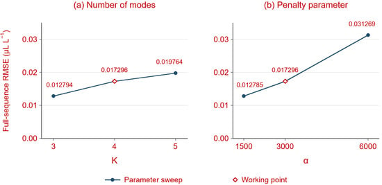
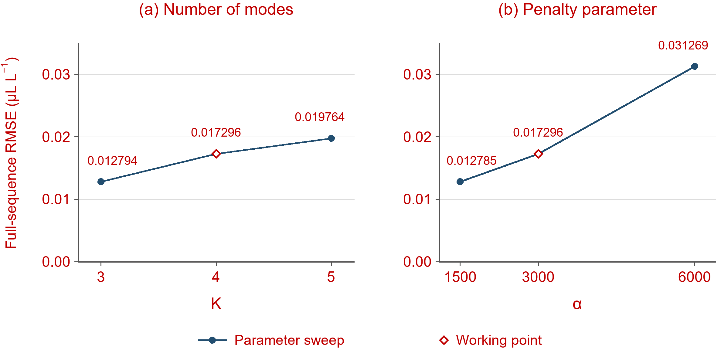
Figure 10 presents the reported sensitivity results for K and α. For K = 3, 4, and 5, RMSE values were 0.012794, 0.017296, and 0.019764 μL·L−1, respectively. Therefore, K = 3 gave the lowest reconstruction error among these three settings. The adopted K = 4 was selected using the training data decomposition criterion described in Section 2.1, which considers modal overlap and frequency uniformity together with the coefficient of variation of adjacent center frequency intervals, rather than minimizing test RMSE.
Figure 10.
Sensitivity of full-test sequence RMSE to (a) VMD mode number K and (b) penalty parameter α. Diamonds mark the working settings K = 4 and α = 3000; neither is the minimum RMSE setting in the tested range.
For α = 1500, 3000, and 6000, RMSE values were 0.012785, 0.017296, and 0.031269 μL·L−1, respectively. Increasing α to 6000 therefore degraded performance in this test. Although α = 1500 achieved the lowest RMSE among the tested settings, the working value α = 3000 was retained to balance reconstruction accuracy with the bandwidth-control role of the VMD penalty parameter. This choice reflects the decomposition considerations of the adopted configuration rather than optimization solely for the minimum test-set RMSE.
For random seeds 42, 43, and 44, the reported RMSE values were 0.017296, 0.016696, and 0.015220 μL·L−1, respectively. Their mean and sample standard deviation were 0.016404 ± 0.001068 μL·L−1, illustrating variation associated with randomness.
3.1.6. Evaluation of KDE-Based Thresholds
To justify the choice of the KDE-based reconstruction error threshold, Table 5 presents the full-sequence RMSE and the number of incorrectly repaired uncorrupted samples at different quantile levels.
Table 5.
Effect of the KDE upper quantile on full-sequence RMSE and the number of uncorrupted samples falsely repaired.
Table 5 evaluates the effect of changing q. At q = 0.90, the full-sequence RMSE was 0.034855 μL·L−1, and five uncorrupted points were falsely repaired. Raising q to 0.94 reduced these values to 0.022847 μL·L−1 and one false repair. For q = 0.96, 0.98, and 0.99, the reported RMSE was identical at 0.017296 μL·L−1, with no false repairs. Thus, the lower tested quantiles caused unnecessary repairs, whereas the three higher quantiles formed a performance plateau in this experiment.
The adopted q = 0.98 represents a practical compromise between avoiding excessive corrections at lower quantiles and maintaining a moderately conservative detection threshold. The identical results obtained at q = 0.96, 0.98, and 0.99 further indicate that the cleaning performance is relatively insensitive to the threshold choice within this tested range.
3.2. Evaluation and Validation of the Decision Model
To validate the evaluation and decision-making model, phase A of main transformer no. 3 at a UHV substation (ODFPS-1000000/1000) was selected as the case study. Multidimensional condition parameters, including operating oil temperature, winding direct-current (DC) resistance, and high-frequency partial discharge, were fed into the model. Among these, anomalies were identified in the operating oil temperature, winding temperature, DC resistance of the main winding, the rate of change in the peak value of high-frequency partial discharge, and the dielectric loss of the main winding and bushings.
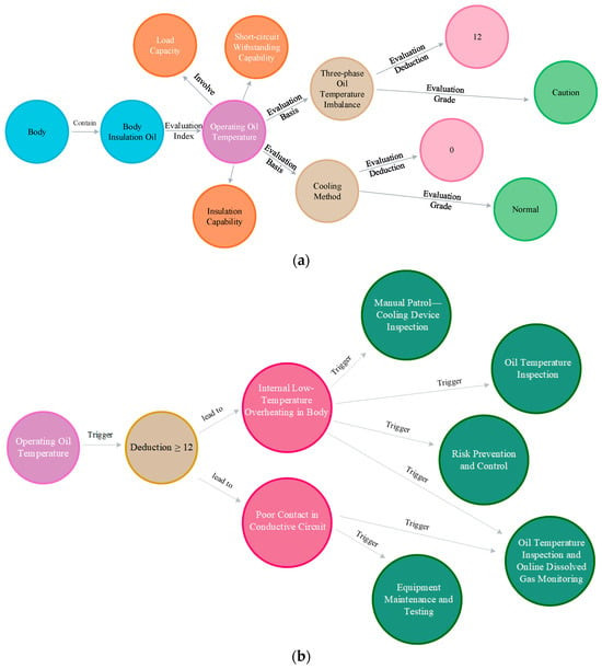
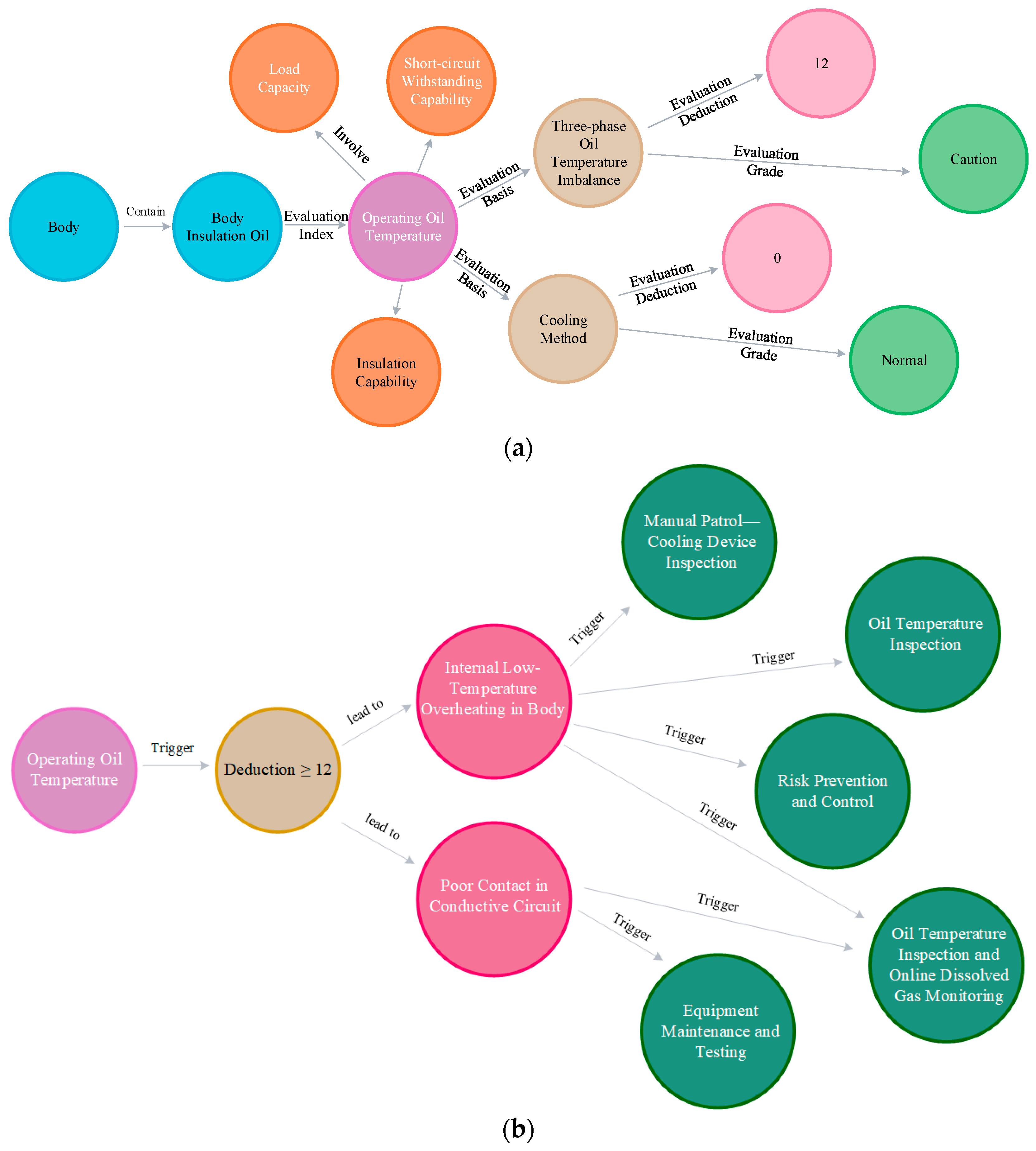
Taking “operating oil temperature” as an example, although the absolute values of the three-phase oil temperatures did not exceed the 75 °C limit, the three-phase temperature imbalance rate exceeded 5% (Phase A: 33.9 °C, Phase B: 38.3 °C, Phase C: 23.8 °C), thereby triggering the “caution” status determination rule and resulting in an automatic deduction of 12 points for this condition parameter. Upon detecting this anomaly, the model initiated knowledge graph-based reasoning, with the results presented in Figure 11a. First, the reasoning confirmed that the anomaly was physically associated with the “body” component. Subsequently, according to the evaluation mapping rules in the knowledge graph, the anomaly was identified as a key evaluation indicator, directly linked to two core dimensions: “insulation capability” and “load capability”. Further reasoning revealed that this anomaly primarily triggered the penalty item for “three-phase oil temperature imbalance,” while the indicators related to the “cooling method” remained normal. This cross-mapping from a single condition parameter to multidimensional capabilities clearly revealed the complex impact pathways of equipment anomalies.
Figure 11.
Visualization of the knowledge graph reasoning process. (a) Condition assessment reasoning from state quantities to capabilities; (b) fault diagnosis and O&M decision-making reasoning.
The remaining three items were evaluated independently: the high-frequency (HF) partial discharge peak change rate was rated “abnormal”, resulting in a 24-point deduction; the winding DC resistance was rated “caution”, resulting in a 12-point deduction; and the dielectric loss of the main winding and bushings was also rated “caution”, resulting in a 12-point deduction. The overall reasoning logic is as follows: Upon receiving an abnormal event for a condition parameter such as “operating oil temperature,” the model first precisely traces the anomaly to the corresponding physical component based on the “component–condition parameter” topological relationships defined in the knowledge graph. Next, following the “capability–component–condition parameter” path, the model further associates the anomaly with core dimensions such as “insulation capability” and “load capability.” Finally, based on the predefined deduction rules in the knowledge graph, the deduction scores for each component are aggregated to compute the equipment’s final score for the corresponding capability dimension.
Based on the above reasoning path, the major components are rated and scored by integrating the analysis results of the multidimensional operational capability evaluation system with expert experience. The evaluation results for the main body of this UHV transformer are summarized in Table 6.
Table 6.
Capability and component ratings and scores for main transformer no. 3 at a certain substation.
The results showed that, due to the combined effects of “abnormal operating oil temperature” (12 points deducted) and “high-frequency partial discharge” (24 points deducted), the equipment’s insulation capability and load capability scores dropped significantly to 70 points, and the rating was downgraded to “caution.”
Upon determining that the equipment is in the “caution” state, the diagnostic module retrieves the expert-assigned values linking the observed abnormal events to potential failure modes. Table 7 presents these single-event values relevant to the case, rather than the results of multi-event fusion.
Table 7.
Expert-assigned association values between potential equipment failure modes and abnormal events.
The event–fault relationships in Table 7 link the observed abnormalities to potential failure modes requiring further investigation and provide a basis for retrieving corresponding maintenance recommendations from the knowledge graph.
By integrating the multidimensional capability assessment, component condition rating, scoring, and fault diagnosis results, the system intelligently matched typical O&M scenarios to generate targeted handling strategies and visualized the process from abnormal events to decision-making using the knowledge graph. For the operating oil temperature anomaly, the decision-making module matched the corresponding handling strategy in the knowledge graph, with the visualization results shown in Figure 11b. The system automatically generated five differentiated O&M recommendations: “intelligent patrol–oil temperature inspection,” “comprehensive maintenance–equipment maintenance and testing,” “manual patrol–cooling device defect,” “intelligent patrol–oil temperature inspection with tracking of dissolved gas online monitoring data,” and “risk prevention and control.” The interpretability of this process is supported by explicit knowledge graph relationships linking observed condition parameters, assessment criteria, affected capabilities, candidate failure modes, and recommended maintenance measures. These relationships allow O&M personnel to inspect the assessment and diagnostic basis associated with the recommendations, supporting their review before implementation.
Based on the equipment condition assessment and fault diagnosis results, a differentiated operation, maintenance, and repair plan was proposed to address abnormal condition parameters and potential failure modes in ultra-high-voltage transformers. This plan encompasses both live-line inspections and de-energized tests, closely aligns with the requirements of the Code for Condition-Based Maintenance Testing of Power Transmission and Transformation Equipment and the Code for Preventive Testing of Power Equipment, and demonstrates high target specificity and practicality.
4. Conclusions
This paper presents a systematic study of the condition assessment and decision-making framework for ultra-high-voltage transformers. To address challenges including the poor quality of online monitoring data and the difficulty in leveraging operation and maintenance decision-making systems, this work proposes a collaborative data cleaning method that exploits the synergy between VMD and SDAE. A domain-specific knowledge graph for UHV transformers is then constructed, transforming scattered regulations, guidelines, expert experience, and equipment ledgers into a structured semantic network. Finally, a condition assessment and knowledge-driven diagnostic and decision-making model grounded in multidimensional capability assessment is established. Experimental results demonstrate the following:
- (1)
- Effective data cleaning performance. Data cleaning performance was assessed using controlled ablations, multiple contamination conditions, parameter sensitivity, and KDE quantile analysis. In the baseline ablation, VMD–SDAE achieved a full-sequence RMSE of 0.017296 μL·L−1, approximately 4.85% lower than the variant without VMD. The clearest advantage among the tested conditions occurred under mixed contamination; improvements were not uniform across Gaussian noise, spikes, long gaps, and genuine step changes. The results also identified sensitivity to the VMD penalty parameter.
- (2)
- Knowledge graph visualization. Leveraging the Neo4j graph database, structured storage and visual querying of knowledge were achieved, successfully transforming fragmented regulations and guidelines into an interactive, visual knowledge network that serves as the knowledge foundation for condition assessment and decision-making.
- (3)
- Interpretable capability assessment and O&M decision support. The case study indicates that the evaluation results produced using the proposed model are reasonable and align with the on-site judgments of operation and maintenance personnel. The model is capable of performing fault analysis based on abnormal condition events and recommending differentiated operation, maintenance, and repair strategies. These recommendations effectively inform actual production and maintenance scheduling, demonstrating considerable engineering applicability.
Despite the promising results, several limitations remain. The case study illustrates the diagnostic reasoning and recommendation-generation processes. Owing to the limited availability of confirmed historical faults, the expert-assigned association values and their fusion results have not undergone statistical calibration or independent diagnostic validation. Further assessment against independently confirmed fault records is required. Although the condition assessment model offers high interpretability, its iteration cycle is relatively lengthy, hindering automatic adaptation to condition changes induced by equipment aging. Future work could focus on establishing a closed-loop feedback mechanism that feeds actual maintenance outcomes back into the model as correction variables, continuously validates logical assumptions and optimizes model parameters using measured data, and thereby improves both the accuracy of diagnostic results and the relevance of maintenance recommendations. Specifically, inspection findings, confirmed fault causes, and post-maintenance monitoring data could be compared with the corresponding model outputs to identify recurrent discrepancies. These findings could guide expert review and revision of the assessment rules and expert-assigned association values, with any changes to thresholds and deductions checked against the applicable guidelines. The updated model should then be evaluated on independent cases to determine whether the revisions improve diagnostic accuracy and the appropriateness of maintenance recommendations.
Future research will also investigate the adaptability and scalability of the proposed framework across transformers with different designs and operating profiles. Potential extensions include temporal knowledge representation, graph-based representation learning, and the integration of physical models to improve diagnostic reasoning under limited fault data. For practical deployment, particular attention should be given to data integrity, computational efficiency, and expert supervision of high-impact maintenance decisions.
In summary, the integrated solution proposed in this paper—combining data cleaning, domain knowledge graphs, and intelligent evaluation and decision-making—delivers not only robust performance in data fidelity and evaluation objectivity but also strong logical interpretability and engineering feasibility. It provides a novel and reliable technical foundation for the online condition monitoring, precise fault diagnosis, and scientific operation and maintenance decision-making of ultra-high-voltage transformers.
Author Contributions
Conceptualization, P.X.; methodology, P.X. and Z.T.; software, Y.Z. and Y.W.; validation, Y.Z.; formal analysis, Y.Z. and F.L.; investigation, Y.Z.; resources, Y.Z. and F.L.; data curation, Y.Z., Y.W., and F.L.; writing—original draft, P.X.; writing—review and editing, P.X.; supervision, P.X. and Z.T.; project administration, P.X.; funding acquisition, P.X. All authors have read and agreed to the published version of the manuscript.
Funding
This work was supported by the Science and Technology Projects of State Grid Hunan Electric Power Co., Ltd. (No. 5216A5250017).
Data Availability Statement
The raw data supporting the conclusions of this article will be made available by the authors on request.
Conflicts of Interest
Authors X.P., Y.Z., Y.W. and F.L. are employed by the company State Grid Hunan Electric Power Co., Ltd. The authors declare that this study received funding from State Grid Hunan Electric Power Co., Ltd. The funder was not involved in the study design, collection, analysis, interpretation of data, the writing of this article or the decision to submit it for publication.
Abbreviations
The following abbreviations are used in this manuscript:
| UHV | Ultra-High Voltage |
| O&M | Operation and Maintenance |
| VMD | Variational Mode Decomposition |
| SDAE | Stacked Denoising Autoencoders |
| RMSE | Root Mean Square Error |
| MAPE | Mean Absolute Percentage Error |
| IoT | Internet of Things |
| IMFs | Intrinsic Mode Functions |
| KDE | Kernel Density Estimation |
| DC | Direct Current |
| HF | High Frequency |
References
- Liu, Z. Innovation practice of ±1100kV ultra-high-voltage DC transmission engineering. CSEE J. Power Energy Syst. 2020, 40, 7782–7792. [Google Scholar] [CrossRef]
- Han, X.; Sun, X.; Chen, H.; Qiu, N.; Lu, D.; Wang, N.; Wang, X.; Zhang, J. Overview of development of UHV AC transmission technology in China. CSEE J. Power Energy Syst. 2020, 40, 4371–4386,4719. [Google Scholar] [CrossRef]
- Li, S.; Li, J. Condition monitoring and diagnosis of power equipment: Review and prospective. High Volt. 2017, 2, 82–91. [Google Scholar] [CrossRef] [Scilit]
- Huyghues-Beaufond, N.; Tindemans, S.; Falugi, P.; Sun, M.; Strbac, G. Robust and automatic data cleansing method for short-term load forecasting of distribution feeders. Appl. Energy 2020, 261, 114405. [Google Scholar] [CrossRef] [Scilit]
- Zhang, X.; Wu, J.; Xuan, X.; Wang, J.; Zhao, X.; Yang, J. Research on Anomaly Detection Method for Virtual Power Plant Measurement Data Based on Isolation Forest Algorithm. In Proceedings of the 2024 6th International Conference on Intelligent Control, Measurement and Signal Processing (ICMSP), Xi’an, China, 29 November–1 December 2024; IEEE: New York, NY, USA, 2024; pp. 253–256. [Google Scholar] [CrossRef] [Scilit]
- Xie, T.; Li, B.; Zhen, Y.; Wei, H.; Xu, K.; Huang, J. Anomaly detection method for power dispatch streaming data based on adaptive isolation forest and self-supervised learning. Front. Phys. 2025, 13, 1704495. [Google Scholar] [CrossRef] [Scilit]
- Li, Z.; Liu, J.; Lin, Y.; Wang, F. Grid-constrained data cleansing method for enhanced bus load forecasting. IEEE Trans. Instrum. Meas. 2021, 70, 1–10. [Google Scholar] [CrossRef] [Scilit]
- Berghout, T.; Lim, W.H.; Amirat, Y.; Tayeb, F.; Benbouzid, M. Exploratory data analysis and recurrent expansion for power systems cybersecurity forensics. In Proceedings of the IECON 2024-50th Annual Conference of the IEEE Industrial Electronics Society, Chicago, IL, USA, 3–6 November 2024; IEEE: New York, NY, USA, 2024; pp. 1–6. [Google Scholar] [CrossRef] [Scilit]
- Mantach, S.; Lutfi, A.; Moradi Tavasani, H.; Ashraf, A.; El-Hag, A.; Kordi, B. Deep learning in high voltage engineering: A literature review. Energies 2022, 15, 5005. [Google Scholar] [CrossRef] [Scilit]
- DL/T 1685-2017; Condition Assessment Guide for Oil-Immersed Transformers (Reactors). National Energy Administration: Beijing, China, 2017.
- DL/T 1723-2017; Technical Guide for Condition-Based Maintenance of 1000 kV Oil-Immersed Transformers (Reactors). National Energy Administration: Beijing, China, 2017.
- Yan, Y. Research on Transmission and Transformation Equipment Status Evaluation Method Based on Big Data Analysis Technology. Ph.D. Thesis, Shanghai Jiao Tong University, Shanghai, China, 2018. [Google Scholar] [CrossRef]
- Wang, J.; Wang, X.; Ma, C.; Kou, L. A survey on the development status and application prospects of knowledge graph in smart grids. IET Gener. Transm. Distrib. 2021, 15, 383–407. [Google Scholar] [CrossRef] [Scilit]
- Yeji, L.; Minjae, S.; Kyungnam, P.; Kim, M.; Song, K.; Lee, H.; Kim, H. Power system decision making in the age of deep learning: A comprehensive review. Energies 2025, 18, 4867. [Google Scholar] [CrossRef] [Scilit]
- Alhamrouni, I.; Abdul Kahar, N.H.; Salem, M.; Swadi, M.; Zahroui, Y.; Kadhim, D.J.; Mohamed, F.A.; Alhuyi Nazari, M. A comprehensive review on the role of artificial intelligence in power system stability, control, and protection: Insights and future directions. Appl. Sci. 2024, 14, 6214. [Google Scholar] [CrossRef] [Scilit]
- Zhang, H.; Zhu, S.; Zhang, Y.; Zhang, L. Research and implementation of condition-based maintenance technology system for transmission and transformation equipment. Power Syst. Technol. 2009, 33, 70–73. [Google Scholar] [CrossRef]
- Silva, N.S.; Castro, R.; Ferrão, P. Smart grids in the context of smart cities: A literature review and gap analysis. Energies 2025, 18, 1186. [Google Scholar] [CrossRef] [Scilit]
- Gazzotti, R.; Faron, C.; Gandon, F.; Lacroix-Hugues, V.; Darmon, D. Extending electronic medical records vector models with knowledge graphs to improve hospitalization prediction. J. Biomed. Semant. 2022, 13, 6. [Google Scholar] [CrossRef] [Scilit]
- Nie, Q.; Geng, J.; Liu, C. A review of fault diagnosis methods: From traditional machine learning to large language model fusion paradigm. Sensors 2026, 26, 702. [Google Scholar] [CrossRef] [Scilit]
- Wang, S.; Zheng, S.; Liu, Z.; Liu, Y.; Dong, P.; Tao, C.; Yu, Y.; Xue, A. Entity relation extraction for knowledge graph construction of relay protection device defects in a regional power grid. Power Syst. Technol. 2023, 47, 1874–1887. [Google Scholar] [CrossRef]
- Liu, P.; Qian, L.; Zhao, X.; Tao, B. Joint knowledge graph and large language model for fault diagnosis and its application in aviation assembly. IEEE Trans. Ind. Inform. 2024, 20, 8160–8169. [Google Scholar] [CrossRef] [Scilit]
- Chen, Q.; Li, Q.; Wu, J.; Mao, C.; Peng, G.; Wang, D. Application of knowledge graph in power system fault diagnosis and disposal: A critical review and perspectives. Front. Energy Res. 2022, 10, 988280. [Google Scholar] [CrossRef] [Scilit]
- Wang, J.; Yang, J.; Pei, Y.; Zhan, X.; Zhou, T.; Xie, P. Research on knowledge graph-based auxiliary decision-making for distribution network faults. Power Syst. Technol. 2021, 45, 2102–2112. [Google Scholar] [CrossRef]
- Shu, S.; Chen, Y.; Zhang, Z.; Fang, S.; Wang, G.; Zeng, J. Construction method of transformer operation state portrait based on multi-dimensional capability and knowledge graph-multilayer perceptron. Power Syst. Technol. 2024, 48, 750–759. [Google Scholar] [CrossRef]
- Zhou, C.; Li, X.; Jiao, R.; Kaihang, L. Joint reasoning for transformer fault diagnosis based on domain knowledge graph. Proc. CSEE 2025, 45, 2160–2171. [Google Scholar] [CrossRef]
- Liu, L.; Wang, B.; Ma, F.; Zheng, Q.; Yao, L.; Zhang, C.; Mohamed, M.A. A concurrent fault diagnosis method of transformer based on graph convolutional network and knowledge graph. Front. Energy Res. 2022, 10, 837553. [Google Scholar] [CrossRef] [Scilit]
- Zhu, B.; Xian, R.; Fan, H.; Liu, X.; Gao, H.; Chen, L. Transformer fault diagnosis technology based on WRSR and improved naive Bayes. Power Syst. Prot. Control 2021, 49, 120–128. [Google Scholar] [CrossRef]
- Xu, B.; Han, X.; Sun, H.; Zhang, Y. Decision-making model for power equipment condition-based maintenance under partially observable conditions. Proc. CSEE 2018, 38, 4107–4116. [Google Scholar] [CrossRef]

Disclaimer/Publisher’s Note: The statements, opinions and data contained in all publications are solely those of the individual author(s) and contributor(s) and not of MDPI and/or the editor(s). MDPI and/or the editor(s) disclaim responsibility for any injury to people or property resulting from any ideas, methods, instructions or products referred to in the content. |
© 2026 by the authors. Licensee MDPI, Basel, Switzerland. This article is an open access article distributed under the terms and conditions of the Creative Commons Attribution (CC BY) license.