


Abstract
A three-dimensional finite-difference model is developed to evaluate reservoir-pressure support by an injection–production well pair. Selected inputs from the Kyrtaelskoye field define a 500 × 200 × 200 m section with constant directional filtration and well-response coefficients. Injection scenarios are compared by the production-zone pressure deficit and a prescribed injection-zone pressure ceiling. At the selected nominal rate of 17.73 m3/h, the production-point pressure is 28.525 MPa and the injection-point maximum is 43.123 MPa against a ceiling of 43.2 MPa. Relative to 10.67 m3/h, the production-point pressure deficit decreases from 0.350 to 0.275 MPa, or by 21.4%, with pressure behavior examined over 24 and 720 h. Independent verification of the diffusion operators confirms second-order spatial and first-order temporal accuracy on an exact-solution test. Analytical reanalysis of the reported scenarios gives an injection-point pressure response of approximately 0.820 MPa per m3/h and quantifies how the admissible rate changes with the injection-response coefficient. The approach connects local pressure support with the operating constraints relevant to subsequent assessment of productive field life.
1. Introduction
Effective management of oil field development is a key factor in ensuring energy security and sustainable economic development. One of the most pressing problems in this area is the assessment and extension of field operating life [1], which directly depends on the dynamics of reservoir pressure and the water cut level of the produced fluids. A decrease in reservoir pressure during operation leads to a decline in well flow rates, deterioration of economic indicators and, as a consequence, a reduction in the field life cycle.
Reservoir pressure maintenance systems, including waterflooding, are widely used to sustain production as reservoir energy is depleted [2,3]. Their performance depends on reservoir properties, well placement and injection–production allocation. Existing numerical and streamline-based approaches already represent well interactions and support rate selection [4,5]. For the present study, the practical task is to compare injection scenarios for a specified well pair while examining the pressure response at the production-well location together with the local pressure increase near the injector.
The purpose of this work is to develop a spatially distributed pressure calculation for an injection–production well pair and to evaluate injection regimes under a prescribed local pressure constraint. The contribution combines pressure support in the production zone, pressure accumulation near the injector and a quantitative rule for adjusting the selected rate when the injection-response coefficient changes. The model application uses a section parameterized from the Kyrtaelskoye field. Pressure responses over 24 and 720 h provide the hydrodynamic component of an operating-life assessment, linking the choice of injection regime with the pressure conditions supporting continued production.
1.1. Reservoir Pressure Decline, Waterflooding, and Field Operating Life
Field operating life is considered here as the period during which continued production remains economically justified. Its evaluation depends on production performance and the costs of continuing operations.
Waterflooding is used when pressure support and fluid displacement are required to sustain development. The selected pattern and allocation of injection depend on reservoir properties and well connectivity [4,6,7,8].
The economic interpretation of field operating life also depends on how geological information and operating risks enter a development decision. Comparative geological and economic assessment has been applied to uranium deposits in Russia and Iran [9], while risk assessment for hard-to-recover heavy-oil reserves is considered in [10] and operational-risk assessment in mining engineering in [11]. These studies provide a wider resource-management context for distinguishing a physical pressure response from an economically justified period of operation.
An increase in produced-water fraction can reduce the oil production rate and raise water-handling costs, although water cut alone does not define the economic limit of a well or field. Continued operation depends on recoverable oil production, lifting and water-treatment costs, available facilities and the resulting operating margin.
Zapivalov [1] discusses the Verkh-Tarskoye field as an example of development accompanied by a produced-water fraction above 80%. The account refers to hydraulic fracturing in newly drilled wells alongside intensive water injection for pressure maintenance. These operations have different immediate purposes: hydraulic fracturing stimulates flow through the near-well region, while injected water replenishes reservoir energy and displaces fluids [12]. The example illustrates the need to assess their combined consequences. The reported 80% water cut is a description of that field situation and is not adopted here as a universal critical value or an abandonment criterion.
Reservoir pressure is the pressure of fluids within the pore space of the reservoir rock. Its evolution during development depends on withdrawal, injection, fluid and rock storage, and the conditions at the boundaries of the reservoir region [8].
As fluids are withdrawn, the pressure response depends on the available reservoir energy and on pressure support. Water injection, gas injection and combined approaches are selected according to reservoir characteristics and development objectives [12]. During waterflooding, changes in saturation and phase mobility can affect the oil rate and produced-water fraction. Injection management therefore requires consideration of pressure support together with the production response [13,14,15].
The choice of an injection fluid also determines which physical processes require attention. Zharikova et al. [16] and Volokhova et al. [17] examine component recovery in gas-condensate development, while Prishchepa et al. [18] consider phase-state forecasting for hydrocarbon fluids at great depths. Related injection research addresses CO2 mobility control [19], water–gas injection in a carbonate oil–gas–condensate reservoir [20] and non-Newtonian-fluid injection during well workover [21]. These applications involve different compositions and flow properties. The present water-injection calculation isolates the pressure response for a specified fluid and constant coefficients, providing a basis for comparing operating regimes under common assumptions.
It should be noted that the decrease in the well flow rate directly depends on the decrease in the reservoir pressure indicator in the oil well. From all of the above, it can be concluded that water cut, which affects the operating life of the field, and reservoir pressure are interconnected and influence each other.
At a low reservoir pressure indicator, a number of problems arise:
1. A decrease in reservoir pressure may lead to deterioration of well productivity and a reduction in total oil production.
2. Changes in pressure gradients may affect water movement toward producing wells; their consequences depend on reservoir connectivity and the production regime.
3. If pressure falls below the bubblepoint, gas liberation can change fluid mobility and the conditions of inflow.
4. Pressure changes may contribute to deposition problems when the fluid composition and temperature conditions favor precipitation.
5. The relative mobility of the flowing phases can change as pressure and saturation evolve.
6. Changes in pressure can alter phase behavior, with consequences for fluid mobility and well inflow.
7. Changes in reservoir and flowing pressures can require adjustment of artificial-lift operating conditions.
8. Gas released during pressure decline can affect the operation of the well and pumping equipment.
9. Improper maintenance of reservoir pressure by means of water injection through an injection well may cause a reduction in the operating life of the field.
These effects can change operating costs and production performance. Selecting a pressure-maintenance regime therefore requires a specified operating objective and an assessment of reservoir and well conditions.
As noted above, over the course of field development, reservoir pressure in the deposit decreases, which leads to a decrease in the oil recovery factor. That is why, for efficient operation of a field, it is necessary to maintain a certain value of reservoir pressure. For this purpose, reservoir pressure maintenance systems are created.
A reservoir pressure maintenance system is a set of methods and technologies aimed at the process of maintaining pressure in the productive reservoir by artificial or natural methods. This is necessary to ensure high rates and sustainable oil production. The methods of maintaining reservoir pressure by means of waterflooding in oil fields will be considered below.
A number of methods are used in oil fields to maintain reservoir pressure using waterflooding.
1. The method of peripheral waterflooding.
The method of peripheral waterflooding was first applied at the Tuymazinskoye field in 1948. This field became the first research object for the development of reservoir pressure maintenance technologies in combination with waterflooding methods [22]. When applying the method of peripheral waterflooding, water injection into the productive reservoir is carried out through injection wells located outside the oil-bearing zone, beyond the external contour, at a certain distance. The distance at which the injection line is placed depends on the degree of exploration of the deposit, the planned distance between injection wells, the distance between the external and internal oil-bearing contours, as well as the distance between the internal oil-bearing contour and the first row of production wells. In addition, there is a method for layer-by-layer distribution of injection for low-permeability formations, taking into account the connectivity of sand bodies and the differences between layers [23].
2. The method of near-contour waterflooding. Injection wells are drilled between the internal and external oil-bearing contours. This method does not make it possible to achieve the maximum production level in a short time, but it can stabilize a high well flow rate for quite a long period.
3. In-contour waterflooding. In this case, water is injected directly into the oil-saturated part of the reservoir.
The efficiency of applying waterflooding methods is assessed according to the following criteria:
1. Positive influence of injection wells on the operation of production wells, an increase in the hydrocarbon recovery factor.
2. Ensuring maintenance of optimal pressure in the reservoir.
3. The relationship between the volume of injected water and the flow rate of the production well.
4. Feasibility of implementing the measures. Assessment of costs and profitability indicator.
At the field-development stage, rate selection is considered alongside water sourcing and management. Golovina and Grebneva [24] discuss groundwater abstraction and protection in transboundary aquifers. For oilfield pressure-maintenance practice, mineralized groundwater use and compatibility between formation and injected waters are considered in [6,7]. These questions concern the water-supply conditions accompanying an injection program.
A complementary surveillance measure is the voidage replacement ratio (VRR), defined as the ratio of injected to produced fluid volumes evaluated at reservoir conditions over the same period. Its interpretation requires consistent volume conversions and identification of the produced phases. Setiawan et al. [25] combined VRR analysis, pressure surveillance and material-balance modeling when evaluating a carbonate-reservoir water-injection program. VRR describes volumetric compensation over the selected reservoir region, whereas local pressure responses also depend on well positions and flow properties. The present calculation therefore focuses on pressure at the monitored production and injection locations. A reservoir-condition fluid balance supplies the information needed for a phase-resolved VRR, while the present spatial calculation complements this indicator by locating the pressure response within the investigated section.
1.2. Methods for Assessing Reservoir Pressure Maintenance Performance
The efficiency of applying the reservoir pressure maintenance system can be assessed using the following groups of methods:
1. Statistical analysis, involving assessment of the dynamics of oil and water flow rates in production wells, reservoir pressure and oil water cut, and injectivity of injection wells.
2. Hydrodynamic modeling, including the construction of hydrodynamic field models [8], numerical experiments under various development scenarios, and forecasting of technological indicators.
3. Geophysical well surveys.
Correlation and regression methods are used to examine relationships between injection and production indicators. Rank measures, including Spearman and Kendall coefficients, can be compared when assessing those relationships [26]. Regression-based analyses of production and injection have also been reported [27,28,29]. The interpretation depends on the data and observation period; a correlation coefficient alone does not identify the physical mechanism of communication between wells.
In general, statistical analysis methods are widely used as a tool for quantitative assessment and forecasting of technological development parameters, such as reservoir pressure, production volume, and water cut [30,31]. Since field indicators are used as input data, statistical methods do not require significant time and financial costs.
The interpretation of injection–production relationships depends on data quality, the observation period and changes in well operating conditions. Relationships established for a local area also require care when extrapolated to a reservoir with different connectivity or property distributions [32]. Statistical analyses should therefore account for concurrent changes in operating conditions.
Data-driven approaches have also been developed specifically for interwell connectivity. Huang et al. [33] represent multilayer injection–production relationships through an improved graph neural network. Jiang et al. [34] combine a material-balance formulation with a neural network to characterize connectivity and forecast productivity. These studies complement the pressure-based methods by addressing information obtained from well operating histories.
Statistical analyses can therefore be complemented by pressure modeling when the task requires examination of a specified spatial response.
Pressure modeling can also be placed within the wider literature on process control and monitoring. Asadulagi et al. [35] consider lumped and distributed controllers for a hydrodynamic process. Other applications include automatic temperature control in catalytic cracking [36] and deep-learning-based visual inspection of power infrastructure [37]. These works concern distinct control or monitoring tasks, for which the inputs and performance criteria differ from the local reservoir-pressure comparison undertaken here.
For the processes that occur inside the productive reservoir, the concepts and tools of mathematical modeling are applied in the course of modeling development processes [5,38]. Reservoir modeling can be understood as modeling the hydrodynamics of flows in the reservoir.
The basic model of unsteady flow of all phases of liquids and gases in the reservoir is a system of partial differential equations with the corresponding boundary and initial conditions.
Thus, using hydrodynamic modeling of cyclic waterflooding in some sections of the deposit, it was revealed that when water production decreased, an increase in oil production was observed at the Gagarinskoye field. The use of this type of field modeling showed the need to change the stationary type of waterflooding to a cyclic type. However, this had to be done only for those wells where a positive effect of injection on the production well is achieved [13,39,40].
In the work “Analysis and Modeling of Hydrodynamic Processes Using Systems with Distributed Parameters”, the mathematical model describes the relationship between the hydrodynamic parameters of the oil-saturated part of the deposit. After obtaining the modeling results, it was determined that during the operation of a production well, by setting the bottomhole pressure, it is possible to control the rates of change in the head of the oil-water contact. This control method is aimed at increasing the oil recovery factor of the entire field [41].
The objectives of mathematical reservoir modeling:
1. Obtaining a set of output data for use in solving various tasks [8].
2. Studying the characteristics of a reservoir with a single well, a group of wells, or several wells interacting with each other.
3. Studying the mechanics of fluid movement in a porous medium.
4. Planning the course of the oil production process [42].
5. Optimizing the oil production system.
1.3. Existing Hydrodynamic Models and Research Gap
When waterflooding systems are used inefficiently, a number of problems arise. The following section reviews existing solutions to these problems using mathematical modeling.
In 1998, an invention patent was published. The objective of the invention is to increase the oil recovery factor by adding zones with deteriorated reservoir properties to development. The purpose of developing this method is to solve the problem of water distribution in a geologically heterogeneous reservoir. First, data on the deposit after water injection are obtained experimentally. By constructing two-dimensional and three-dimensional mathematical models with previously determined deposit data, zones in which residual oil reserves are concentrated are identified, where the minimum value of the rate of reservoir pressure increase is assumed. After that, additional horizontal wells are drilled in these zones to extract oil [43].
For the waterflooded zones of the Central Aznakaevskaya area, a mathematical modeling method was applied, which makes it possible to study the process of residual reserve depletion in this area [44]. Using the developed model, it is possible to calculate the current field of oil saturation and water saturation, and to forecast the further development process of the area when changing the flow rate values for production wells. After laboratory and experimental studies were carried out, work was conducted to optimize the operation of production wells, and the operation of 3 injection wells was stopped. As a result, it was possible to reduce the water cut of produced hydrocarbons. It was established that the developed model does indeed have forecasting capabilities.
When modeling the process of fluid filtration in the oil reservoir of the Ust-Balykskoye field, a mathematical model of the field was obtained, based on solving the problem of fluid filtration. The mathematical model is solved using the finite difference method. The output data resulting from the modeling are the flow rates of production wells [45].
A field development system was also developed [46]. At the same time, the field development system is considered as a system with distributed parameters. The model obtained in the course of the study makes it possible to forecast changes in reservoir pressure under various well operating modes. The mathematical description of the field section is a filtration equation in three-dimensional space in differential form with partial derivatives. Such a model will make it possible to more accurately determine the change in head at any point of the reservoir.
In 2017, an invention patent was published for a method of controlling waterflooding of oil reservoirs. Mathematical modeling is used to determine the optimal values of the influence of an injection well on a production well. The purpose of modeling is to obtain optimal operating modes of the injection well to ensure the maximum flow rate indicator of the production well. The output data during modeling are the dependence of the production well flow rate on the volume of injected water. The developed mathematical model will increase the reservoir oil recovery factor and improve the efficiency of using the waterflooding system. The method provides a further example of selecting operating regimes through mathematical modeling [47].
Recent work demonstrates several ways to connect water-injection decisions with reservoir responses. Yin et al. [48] used streamline simulation and three-dimensional visualization to examine injection allocation in an irregular horizontal–vertical well pattern, assessing sweep and water-breakthrough behavior. Their allocation problem involves several interacting wells. The present calculation examines a specified pair and compares pressures at the two monitoring locations, with a prescribed local pressure ceiling.
Li et al. [49] investigated mechanisms and influencing factors of high-pressure water injection, emphasizing the need to relate injection behavior to reservoir conditions. Moorman et al. [50] studied intermittent injection cycles in a reservoir-simulation framework that also considered asphaltene-related formation damage. These studies address physical processes and operating decisions beyond the constant-coefficient pressure formulation used here. Their findings help distinguish the physical processes governing pressure support, displacement and production response when selecting the scope of a development model.
Zhao and Qi [12] reviewed water injection, gas injection and fracturing technologies, relating their application to reservoir characteristics and operational limitations. Together with the well-pair approaches in [4,5], these studies provide a basis for interpreting the present pressure-response calculation under its stated conditions. Its specific task is the joint comparison of production-zone pressure support and injection-zone pressure increase for the investigated pair, using explicitly stated parameters and assumptions. The research task addressed here is a transparent local decision procedure: the same parameterized pressure model supplies the production-zone response, the injection-zone constraint and the sensitivity of the nominal rate to the intensity of injection forcing.
2. Materials and Methods
2.1. Study Area and Computational Domain
In order to extend the operating life of a production well, it is necessary to reduce the rate of decline in its flow rate. This can be achieved through the proper use of the reservoir pressure maintenance system by injecting water into the injection well [4,51].
The investigated section contains two neighboring wells, one for injection and one for production. Treating the section as a system with distributed parameters makes it possible to evaluate pressure throughout the calculation domain and to compare the responses at the two wells under common initial and boundary conditions.
The calculation represents a 500 × 200 × 200 m section parameterized using selected inputs from the Kyrtaelskoye field. The initial pressure, storage coefficient, production rate and gas-cap boundary pressure provide the field-based conditions of the example. Reference filtration coefficients and adopted well-response coefficients complete the parameterization. Table 1 distinguishes these input groups and summarizes the numerical settings. The resulting application evaluates the method through a defined field-prototype scenario, with numerical verification and sensitivity assessment described separately in Section 2.4.
Table 1.
Inputs and numerical settings of the reported pressure calculation. Source: compiled by the authors.
2.2. Governing Equation and Boundary Conditions
Compilation of the basic equation for describing the mathematical model of an oil field is based on the application of fundamental physical laws [8], such as:
1. The law of conservation of mass.
2. Darcy’s law, the filtration law.
3. Equations of state, compressibility of rock and fluids.
4. The first law of thermodynamics.
Darcy’s law, or the law of fluid flow in a porous medium, plays the main role in constructing the mathematical model of the field. When studying the flow of water through vertical sand filters, Darcy empirically derived the filtration law.
The filtration law for a homogeneous fluid [8]:
where Vs is the mass velocity in the flow direction s; k is the permeability of the porous medium in the flow direction; m is dynamic viscosity; p is pressure; z is the vertical coordinate; ρ is fluid density; g is gravitational acceleration; v is specific volume, .
The procedure for compiling the basic equation of the mathematical model of an oil reservoir:
1. First, it is necessary to select an element of the system, planar, three-dimensional, or spherical.
2. Then it is necessary to describe all fluid flows entering and leaving the element over a certain period of time.
3. The amount of fluid flowing in and out is equated to changes in mass inside the system during this time, the law of conservation of mass.
4. Then a transition is made to the limits when the volume is contracted to an infinitesimal size.
Thus, after completing all of the above, the basic equation of the mathematical model of the oil field is compiled [46]:
where x, y, z are spatial coordinates; P is reservoir pressure, MPa; n is the coefficient of elastic capacity, 1/MPa; kx, ky, kz are filtration coefficients along the corresponding spatial coordinates, m/h; V(t) is the pressure change caused by well operation; del(x, y, z) is a unit function equal to 0 or 1, depending on the location of the production and injection wells.
The directional coefficients denoted by kx, ky and kz in Equation (2) are filtration coefficients (hydraulic conductivities), expressed in m/h. They are distinguished from the intrinsic permeability in Darcy’s law, which is expressed in m2. For a fluid with specified density and dynamic viscosity, their relation in consistent SI units is , where κ denotes intrinsic permeability. Conductivity reported in m/h must first be converted to m/s when this relation is used with SI fluid properties. Table 1 reports the directional filtration coefficients actually used in the calculation; the conversion relation identifies the fluid properties required when expressing the same parameterization through intrinsic permeability.
The calculation uses constant effective values kx = ky = 3.2 m/h and kz = 2.92 m/h, representing easier filtration along the bedding than across it. The storage coefficient aggregates the pressure-storage response of the section. This parameterization isolates the effect of injection rate at a fixed level of directional anisotropy. Spatial contrasts in reservoir properties would modify local pressure gradients and preferential water movement, while changes in the effective coefficients would alter pressure levels and transient response; these effects define the conditions for transferring the local comparison to another reservoir section.
To construct the mathematical model, it is necessary to set initial and boundary conditions. Under the initial conditions, the time point is equal to 0, and the pressure at each point will be the same:
P(x, y, z, 0) = P0
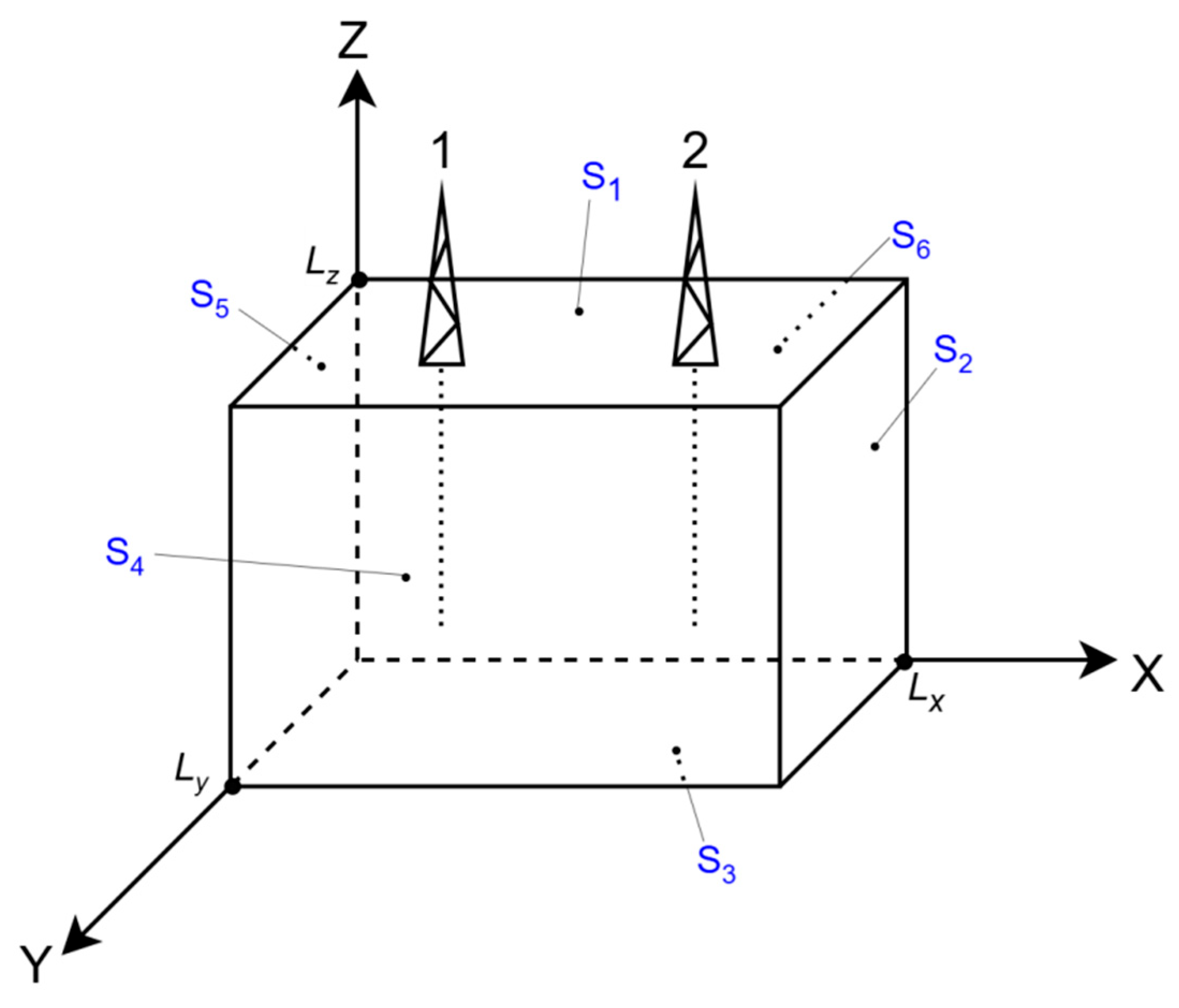
Boundary conditions of the first kind for the plane S1:
P(x, y, Lz, τ) = P1
0 ≤ x ≤ Lx, 0 ≤ y ≤ Ly,τ > 0
Boundary conditions of the first kind for the plane S2:
P(Lx, y, z, τ) = P0
0 ≤ y ≤ Ly, 0 ≤ z ≤ Lz,τ > 0
Boundary conditions of the second kind for the plane S3:
0 ≤ x ≤ Lx, 0 ≤ y ≤ Ly, τ > 0,
Boundary conditions of the first kind for the plane S4:
P(x, Ly, z, τ) = P0,
0 ≤ x ≤ Lx, 0 ≤ z ≤ Lz, τ > 0,
Boundary conditions of the first kind for the plane S5:
P(0, y, z, τ) = P0,
0 ≤ y ≤ Ly, 0 ≤ z ≤ Lz, τ > 0,
Boundary conditions of the first kind for the plane S6:
P(x, 0, z, τ) = P0,
0 ≤ x ≤ Lx, 0 ≤ z ≤ Lz, τ > 0,
Figure 1.
A section of an oil field in three-dimensional space: 1—injection well; 2—production well; Lx—length of the modeled section, m; Ly—thickness of the modeled section, m; Lz—height of the modeled section, m; S1, S2, S3, S4, S5, S6—planes. Source: compiled by the authors.
2.3. Finite-Difference Formulation
To solve this mathematical model, we will apply the finite difference method to write the equation in discrete form. With the help of this method, the continuous distribution of parameters is replaced by a discrete one. When discretizing the required equation, finite-difference equations are obtained.
1. The finite difference method for the X axis.
The first derivative using the backward difference:
The first derivative using the forward difference:
Averaging the backward and forward differences in Equations (16) and (17) gives the central approximation of the first derivative:
Then the analog of the second partial derivative for X:
Having simplified expression (19), we obtain:
2. The finite difference method for the Y axis.
Similarly, we obtain the analog of the second partial derivative for the Y axis:
3. The finite difference method for the Z axis.
Similarly, we obtain the analog of the second partial derivative for the Z axis:
4. The analog of the derivative for :
Taking into account all of the above, when discretizing Equation (2), we obtain:
Then the pressure at a given point of the field section over time can be described by the equation in discrete form:
where Px,y,z,τ is the pressure at a specific point of the reservoir, MPa; n is the coefficient of elastic capacity, 1/MPa; kx, ky, kz are filtration coefficients along the corresponding spatial coordinates, m/h; x, y, z are points on the X, Y, Z axes; ∆x, ∆y, ∆z are discretization steps along the axes; V(t) is the pressure change caused by well operation; del(x, y, z) is a unit function equal to 0 or 1, depending on the location of the production and injection wells.
At the points where the wells are located del(x, y, z) = 1, at the remaining points of the field section del(x, y, z) = 0.
1. The pressure change caused by the operation of the injection well is calculated by the formula:
where f1 is the specific injection resistance, MPa∙h/m3; Q is the flow rate of the injection well, m3/h.
V(t) = f1 ⋅ Q,
2. The pressure change caused by the operation of the production well is calculated by the formula:
where f2 is the specific filtration resistance, MPa∙h/m3; q is the flow rate of the production well, m3/h.
V(t) = −f2 ⋅ q,
The injection and production wells are represented by vertical sets of grid nodes corresponding to their modeled intervals. The indicator del equals one at the relevant well nodes and zero elsewhere. Positive forcing f1Q represents injection and negative forcing −f2q represents production. The coefficients f1 and f2 express the adopted pressure response to well operation at the reported grid and time step. This representation transfers the effect of each well to the surrounding pressure field while keeping the local comparison computationally compact.
Both wells act on the same pressure field P(x,y,z,t). The finite-difference operator transmits the pressure perturbation between neighboring nodes and couples the injection and production locations through the calculation domain. The production rate q is prescribed, so the comparison measures the pressure conditions supporting inflow at that rate. Constant storage gives a linear response, and holding the well-response coefficients fixed provides a common basis for comparing injection scenarios.
The discretization step along the X axis is calculated as:
where Lx is the length of the modeled section, m; p1 is the number of spatial intervals along the x axis, units.
The discretization step along the Y axis is calculated as:
where Ly is the thickness of the modeled section, m; p2 is the number of spatial intervals along the y axis, units.
The discretization step along the Z axis is calculated as:
where Lz is the height of the modeled section, m; p3 is the number of spatial intervals along the z axis, units.
Let us write the boundary conditions in discrete form.
Boundary conditions of the first kind in discrete form for S1:
0 ≤ x ≤ p1, 0 ≤ y ≤ p2, τ > 0,
Boundary conditions of the first kind in discrete form for S2:
0 ≤ y ≤ p2, 0 ≤ z ≤ p3, τ > 0,
Boundary conditions of the second kind in discrete form for S3:
Px,y,0,τ = Px,y,1,τ,
0 ≤ x ≤ p1, 0 ≤ y ≤ p2, τ > 0,
Boundary conditions of the first kind in discrete form for S4:
0 ≤ x ≤ p1, 0 ≤ z ≤ p3, τ > 0,
Boundary conditions of the first kind in discrete form for S5:
P0,y,z,τ = P0,
0 ≤ y ≤ p2, 0 ≤ z ≤ p3, τ > 0,
Boundary conditions of the first kind in discrete form for S6:
Px,0,z,τ = P0,
0 ≤ x ≤ p1, 0 ≤ z ≤ p3, τ > 0,
The mathematical model of the oil field was implemented in Embarcadero C++Builder.
2.4. Numerical Verification and Sensitivity Assessment
The diffusion part of the explicit update can be expressed through the algebraic stencil weights ri = Δt ki/(n Δi2), where i denotes x, y or z. For prescribed well forcing, the homogeneous perturbation equation has a nonnegative central weight when rx + rᵧ + rz ≤ 1/2 [52]. Using the coefficient convention and numerical values of the reported recurrence gives rx = rᵧ = 0.02207 and rz = 0.02014. Their sum is 0.06428 and the central weight is 0.87145, satisfying this stability condition for the diffusion update.
An independent exact-solution test isolates the consistency of the difference operators. On a normalized unit cube, the test equation is uτ = Dx uξξ + Dᵧ uηη + Dz uζζ, with D = (3.2, 3.2, 2.92)/9.32, zero boundary values and initial condition sin(πξ)sin(πη)sin(πζ). Here ξ, η, ζ and τ are normalized coordinates and time, u is the normalized test field, and D contains the normalized directional diffusion coefficients. Since Dx + Dᵧ + Dz = 1, the exact solution is u = exp(−π2τ)sin(πξ)sin(πη)sin(πζ). The centered spatial operator is checked against its discrete mode eigenvalue λh = −4 h−2sin2(πh/2). Spatial refinement uses exact evolution of this discrete mode, and temporal refinement compares forward-Euler evolution with that discrete reference, separating the two error contributions.
The sensitivity assessment uses the linear structure of the fixed-coefficient pressure model and the tabulated stationary response. At fixed geometry, production rate and boundary conditions, injection forcing depends on the product f1Q. A change f1 → αf1 is therefore equivalent, within that parameterization, to Q → αQ. The pressure–rate slope is estimated from Table 2 and used to calculate the pressure change, remaining distance to Pc and corresponding rate bound. This provides an algebraic assessment of injection-response uncertainty for the reported reservoir configuration.
Table 2.
Effect of injection-well flow rate on steady-state pressure at production-well point A and maximum pressure at injection-well point B. Source: compiled by the authors.
3. Results
3.1. Reservoir-Pressure Response at Selected Monitoring Points
The reservoir example uses 50 × 20 × 20 spatial intervals with Δx = Δy = Δz = 10 m over the 500 × 200 × 200 m domain. Accordingly, the boundary indices are x = 0…50, y = 0…20 and z = 0…20. The time step is Δt = 0.001 h and the initial pressure is P0 = 28.8 MPa. Monitoring coordinates are grid indices. The pressure responses are examined over 24 h and, for the selected regime, over 720 h.
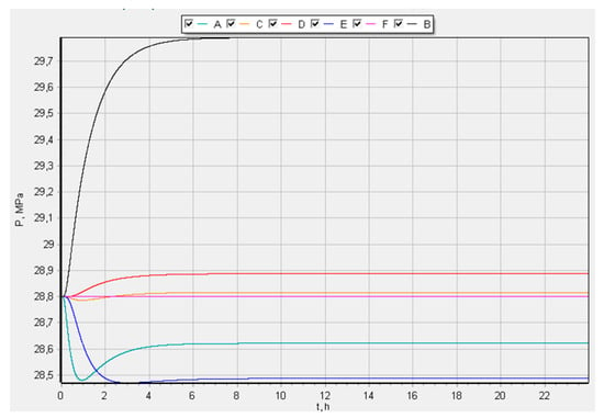
A computational experiment was conducted to obtain the dependence P(t) during the operation of production and injection wells at 6 points with coordinates A (5; 10; 14), B (9; 7; 8), C (25;1;10), D (25;19; 2), E (33;10;10), F (50;15; 3). The selected points do not coincide with the coordinates of the well locations; point F(50;15;3) is a boundary point, lying on the plane S2. Let us take the flow rate of the injection well as Q = 10.67 m3/h.
Using the input data, the resulting pressure curves are presented in Figure 2.
Figure 2.
Reservoir-pressure evolution at monitoring points A–F over 24 h for an injection-well flow rate of Q = 10.67 m3/h.
3.2. Pressure Distribution Along the Injection Well
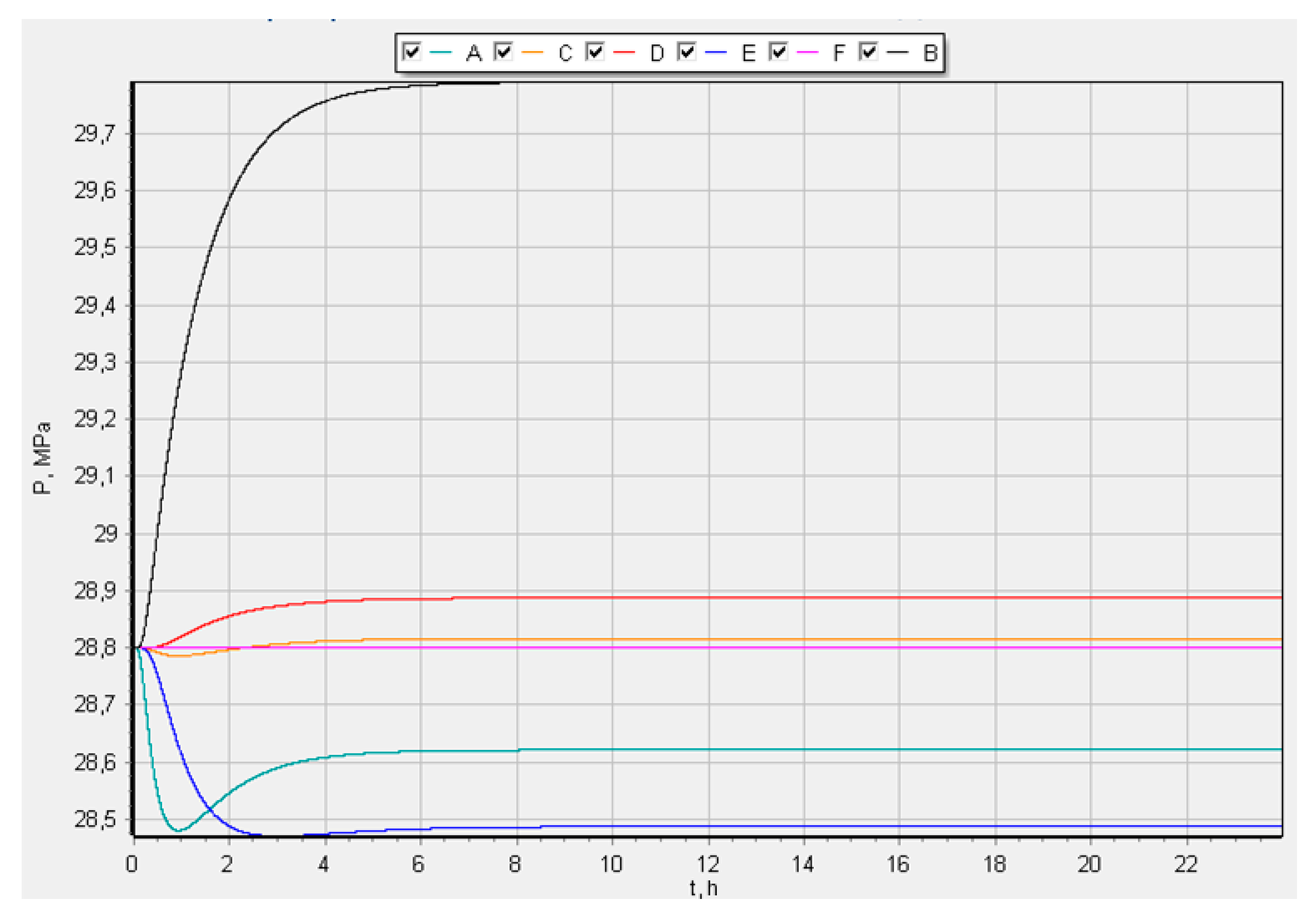
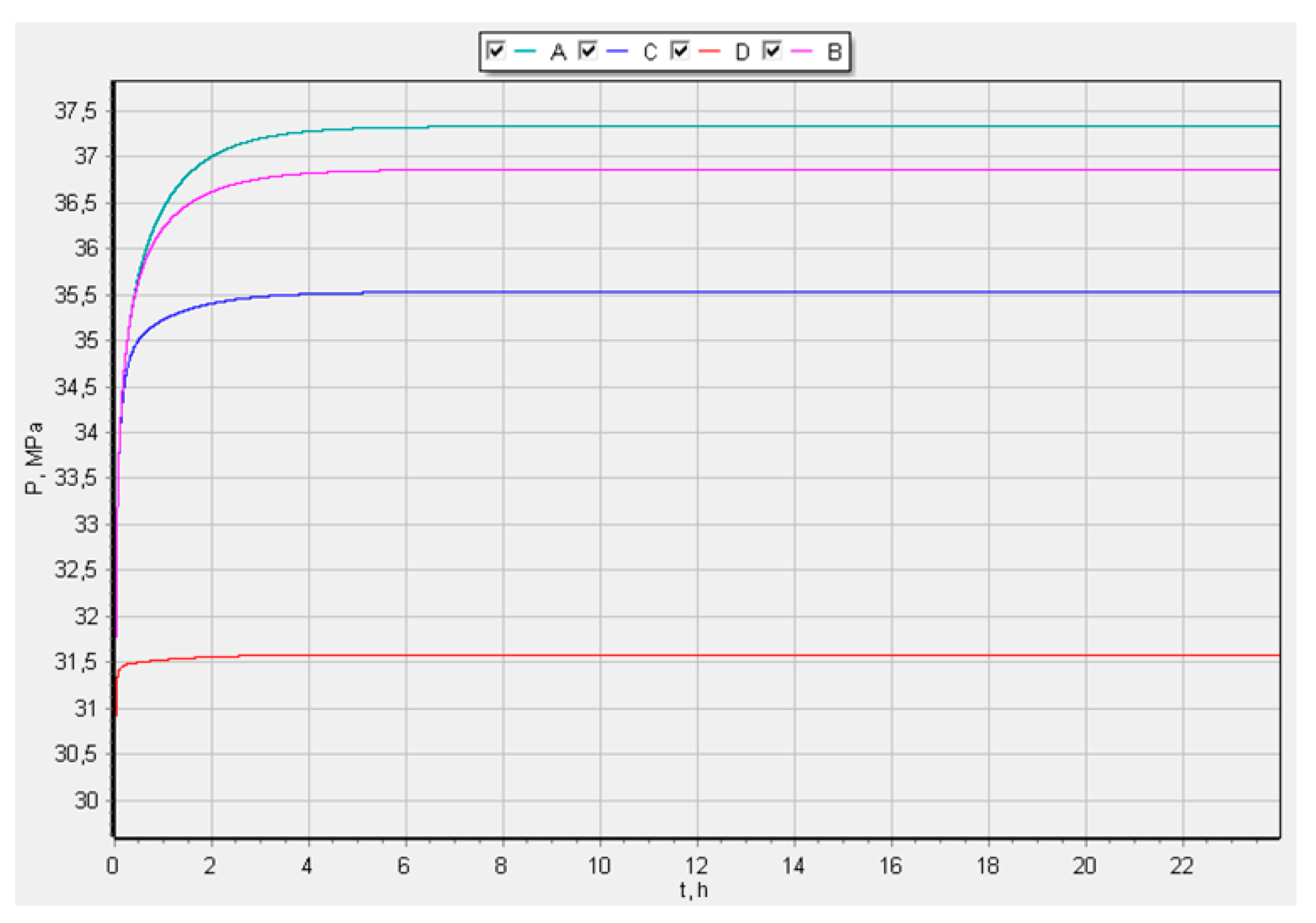
A computational experiment was conducted to obtain the dependence P(t) during the operation of production and injection wells at the points of the injection well location: A (15;10; 5), B (15;10;10), C (15;10;15), D (15; 10; 19). The points are located from the bottomhole to the wellhead Q = 10.67 m3/h.
For the scenario comparison, the pressure ceiling is prescribed as Pc = 1.5 P0 = 43.2 MPa for P0 = 28.8 MPa. This engineering assumption defines a common constraint for selecting the injection regime. In a field application, the ceiling is specified from the local stress state, rock strength and well-test information, preserving the same selection procedure.
The constraint applies to reservoir pressure at a node near the lower injection interval. This location provides the local pressure indicator used in the rate comparison. Its relation to fracture initiation depends on geomechanical conditions and the pressure distribution around the well, as discussed for high-pressure injection in [49,51]. The model therefore treats Pc as an operating constraint on the calculated pressure field.
Figure 3 shows the largest pressure increase near the lower injection-well interval and the smallest increase near the upper interval. The pressures at the monitored points approach steady values and remain below the prescribed ceiling of 43.2 MPa.
Figure 3.
Reservoir-pressure evolution at points A–D along the injection well from the bottomhole to the wellhead over 24 h at Q = 10.67 m3/h.
3.3. Injection-Rate Selection and Long-Term Pressure Response
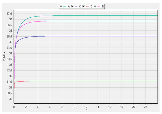
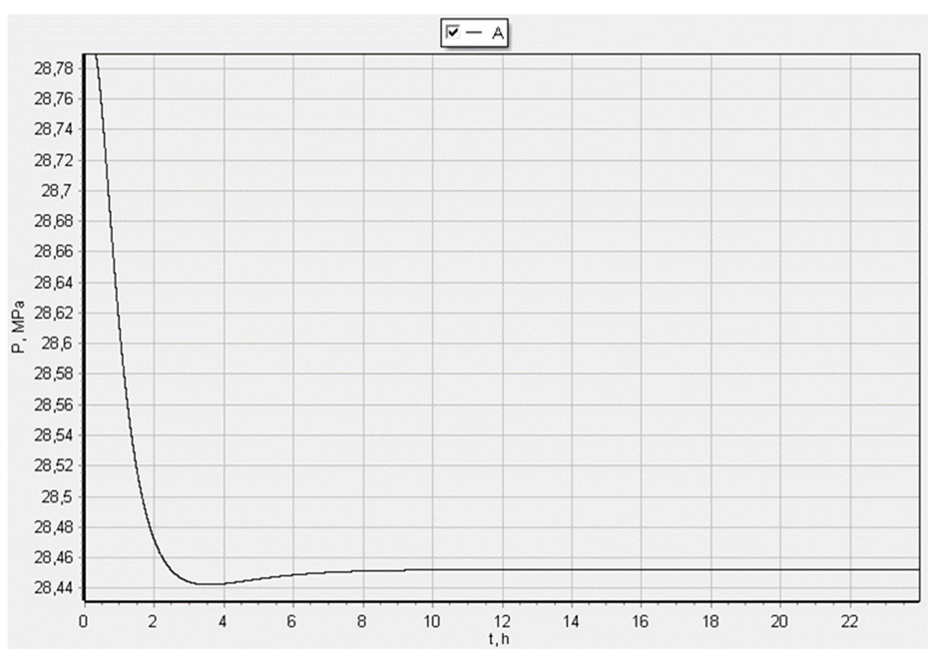
A computational experiment was conducted to obtain the dependence P(t) during the operation of production and injection wells at one of the points of the production well location: A(35;10;10) Q = 10.67 m3/h.
The graph in Figure 4 shows that during the first 3 h, a decrease in reservoir pressure to 28.44 MPa was observed.
Figure 4.
Reservoir-pressure evolution at production-well point A (35, 10, 10) over 24 h at Q = 10.67 m3/h.
However, during the next 3 h, the value reached a steady state of 28.45 MPa. Compared with the initial pressure, 28.8 MPa, the pressure decreased by ΔP = P0 − Ps.s.p. = 28.8 − 28.45 = 0.35 MPa.
The reported scenarios compare injection rates between 12.7 and 17.75 m3/h. The pressure-based performance measure is the decrease from the initial pressure to the steady-state pressure at production-well point A(35,10,10), with a smaller decrease indicating greater pressure support. The comparison is subject to the prescribed condition that pressure at injection-well point B(15,10,5), corresponding to point A in Figure 3, remains at or below 43.2 MPa.
The screening uses nonuniform rate increments and finer sampling near the retained regime, as shown in Table 2. The selection rule first compares the production-point pressure deficit under the prescribed injection-point pressure constraint, then favors the lower rate when two scenarios give the same production-point pressure at the displayed precision. The resulting value is a preferred nominal scenario within the tested set.
The results of the experiment are presented in Table 2.
At Q = 17.73 m3/h, the production-point pressure is 28.525 MPa and the injection-point maximum is 43.123 MPa. At Q = 17.75 m3/h, the displayed production-point pressure remains 28.525 MPa while the injection-point pressure increases to 43.140 MPa. The rate difference is 0.02 m3/h, approximately 0.113%, and the respective distances to the adopted ceiling are 0.077 and 0.060 MPa. The lower rate is retained because it provides the same displayed pressure support with a greater distance to the constraint. The three-decimal reporting precision governs this tie-break. Both scenarios satisfy the specified pressure constraint; their comparison concerns the pressure margin near the injector.
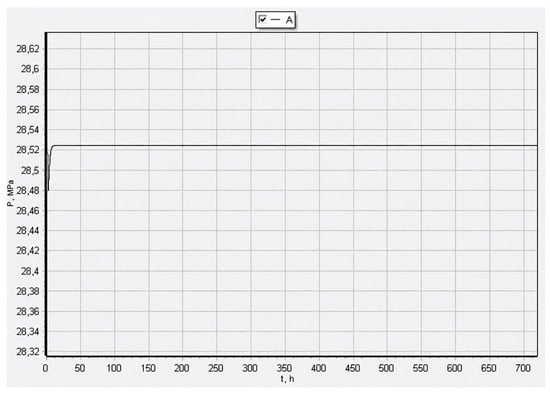
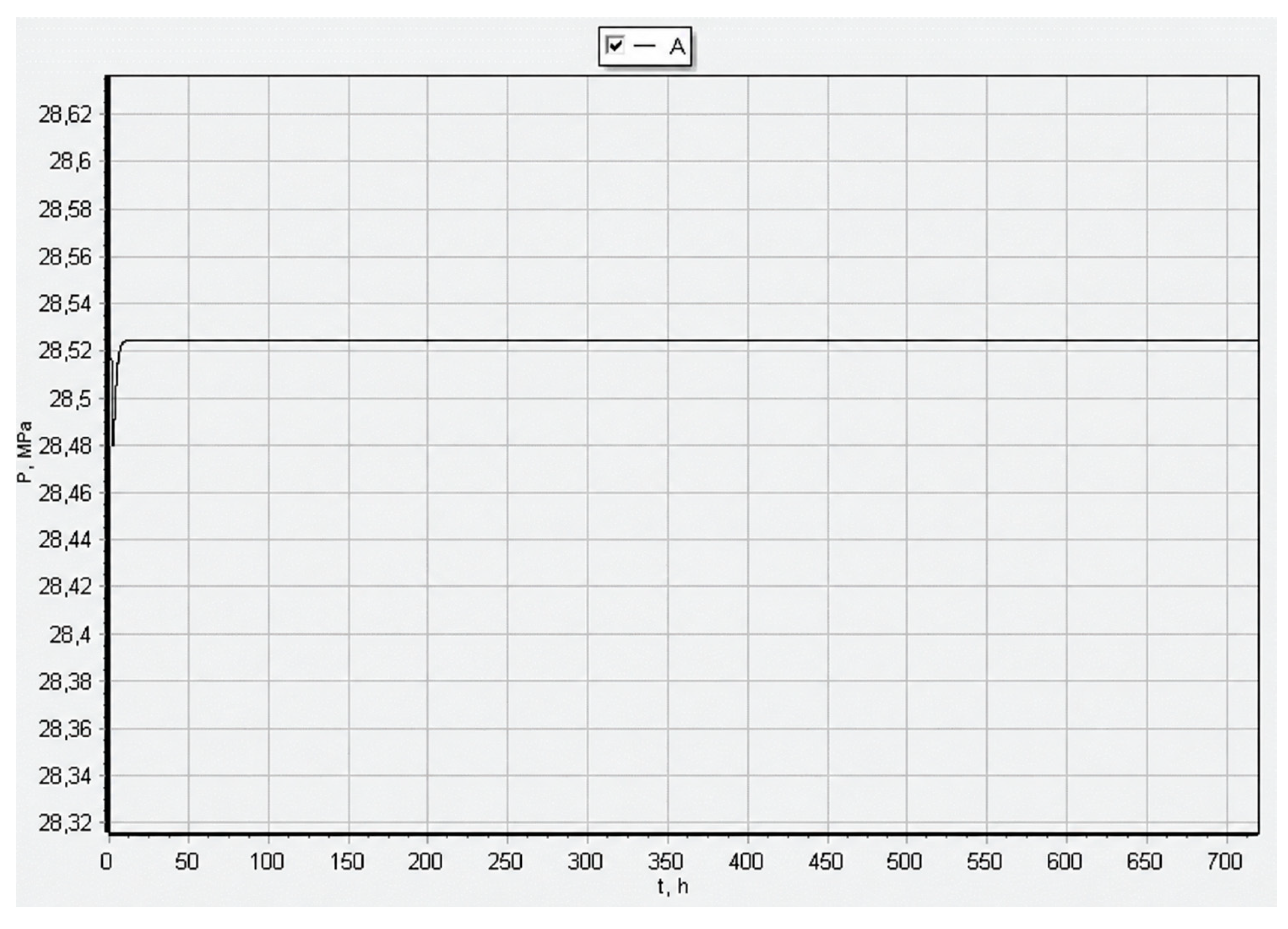
Figure 5 shows a graph of the change in reservoir pressure during well operation over 720 h for point A(35;10;10) at an injection well flow rate of Q = 17.73 m3/h.
Figure 5.
Long-term reservoir-pressure response at production-well point A (35, 10, 10) over 720 h at Q = 17.73 m3/h.
Thus, with the help of the developed model and its software implementation, graphs of the dependence P(t) were obtained at selected points of the modeled field section.
3.4. Verification of the Difference Operators
Table 3 reports the exact-solution test at normalized time τ = 0.05. The spatial errors decrease by approximately four when the mesh spacing is halved, with observed orders of 1.999 and 2.000. At fixed N = 20, where N is the number of intervals per direction, halving the time step approximately halves the temporal error, giving an order of 1.000. Errors are maximum absolute differences over the grid. The test verifies the expected orders of the centered spatial and forward-Euler temporal operators under smooth conditions; the reservoir pressures in Table 2 retain their stated grid, well representation and parameterization.
Table 3.
Independent exact-solution verification of the diffusion operators on the normalized unit cube. Source: calculated by the authors.
3.5. Analytical Sensitivity of the Nominal Injection Regime
The 18 injection scenarios in Table 2 give the stationary relation PB(Q) ≈ a + bQ, with a = 28.57805 MPa and b = 0.820375 MPa/(m3/h). The maximum deviation from the displayed pressures is 0.00046 MPa, consistent with their three-decimal reporting. Here PB denotes pressure at the injection monitoring point, a is the fitted intercept and b is the pressure–rate slope. To retain the tabulated reference exactly, sensitivity is evaluated as PB(αf1,Q) ≈ 43.123 + bQ(α − 1) at Q = 17.73 m3/h (Table 4). The coefficients and other inputs are held fixed, so the estimates describe the effect of injection forcing within the adopted linear formulation.
Table 4.
Algebraic sensitivity to the injection-response coefficient at Q = 17.73 m3/h with the other inputs fixed. The percentages are illustrative perturbations. Source: calculated from Table 2.
Positive and negative values in the last column identify the two sides of the prescribed pressure constraint. The 0.077 MPa nominal margin corresponds to an increase of approximately 0.53% in f1, or the same relative increase in Q with f1 fixed. For an illustrative upper coefficient factor α = 1.15, the same linear relation gives Q ≤ [17.73 + (43.2 − 43.123)/b]/1.15 ≈ 15.50 m3/h. These values are algebraic continuations of the fixed-coefficient model, including effective rates beyond the tabulated range. They show how the pressure constraint adjusts the selected regime under a stated coefficient perturbation. A 0.1 MPa change in Pc corresponds to approximately 0.122 m3/h in the nominal rate bound. The perturbation percentages specify scenarios rather than a statistical distribution of field uncertainty.
4. Discussion
4.1. Interpretation of the Simulated Pressure Response
The conducted computational experiments demonstrated that the pressure response within the modeled field section is spatially nonuniform and depends on the positions of the monitoring points relative to the injection and production wells. At the initial reservoir pressure of 28.8 MPa, the operation of the wells produced both increasing and decreasing pressure trends at different points of the computational domain. The highest pressure increase was observed in the zone affected by the injection well, whereas the pressure decreased at points located closer to the production well. The obtained results confirm that the effect of water injection cannot be evaluated only from an average reservoir-pressure value, since local pressure changes differ substantially within the same modeled section.
The pressure curves obtained for points located along the injection well also showed a clear spatial gradient. The greatest pressure increase occurred near the bottomhole, while lower values were obtained toward the wellhead. Under the initial injection scenario, with a flow rate of 10.67 m3/h, the pressure at all investigated points stabilized below the adopted limit of 43.2 MPa. This result indicates that local bottomhole conditions should be considered when selecting an injection rate. Evaluation based only on the pressure response in the production-well zone would not identify the local increase in pressure near the injection well and the need for a separately justified pressure constraint, as discussed for high-pressure injection in [51].
At production-well point A (35, 10, 10), the reservoir pressure initially decreased from 28.8 to 28.44 MPa and subsequently stabilized at approximately 28.45 MPa. Increasing the injection-well flow rate to 17.73 m3/h raised the calculated steady-state pressure at this point to 28.525 MPa. Consequently, the modeled pressure deficit relative to the initial reservoir pressure decreased from 0.350 to 0.275 MPa, or by approximately 21.4%. At the same time, the maximum pressure at injection-well point B reached 43.123 MPa and remained 0.077 MPa below the adopted pressure constraint.
Over 720 h, equivalent to 30 days, the production-point pressure remains close to the established level under the prescribed regime. Together with the 21.4% reduction in pressure deficit, this result quantifies the pressure support supplied by the selected injection regime. In an operating-life assessment, this pressure trajectory forms the hydrodynamic input to forecasts of production, produced-water fraction and operating costs.
4.2. Comparison with Previous Studies
The well-pair interpretation used here is consistent with existing waterflood-management approaches. Alizadeh and Salek [4] used injector–producer pair recovery factors and water-cut information in a streamline-based allocation method. Zhang and Chen [5] addressed rate allocation over multiple geological realizations with data assimilation. These approaches already connect individual wells and reservoir response. The present calculation focuses on the pressure change at two specified monitoring locations for one adopted parameter set.
Yin et al. [48] considered injection allocation in an irregular well pattern, while the studies in [49,51] examined high-pressure injection mechanisms and reservoir influences. The present constant-coefficient formulation concentrates on pressure transmission within a specified pair. Its practical contribution is the explicit link between two local pressure indicators and a rate-selection rule that can be adjusted through the injection-response coefficient.
The comparison in Section 3.4 evaluates the accuracy of the difference operators against an exact diffusion solution, giving a reproducible reference for the spatial and temporal approximations. The literature comparison addresses the complementary question of model scope: streamline and multiphase approaches resolve allocation or displacement behavior, while the present formulation offers a compact pressure-based calculation for local regime assessment. Computational effort and predictive performance are interpreted with respect to the physical task and the input information used by each approach.
4.3. Practical Implications for Reservoir Pressure Management
For the adopted well pair and parameter set, Q = 17.73 m3/h is the preferred nominal rate under the stated selection rule. It is the lowest sampled rate giving a production-point pressure of 28.525 MPa at the reported precision, while maintaining the injection-point pressure below Pc. The role of this reference value is to demonstrate the rate-selection procedure under specified reservoir and operating conditions.
The analytical sensitivity assessment in Section 3.5 converts the nominal pressure margin into a quantitative adjustment rule. With the other inputs fixed, a 15% increase in the injection-response coefficient gives an upper rate of approximately 15.50 m3/h under the same ceiling. The value 17.73 m3/h and the adjusted bound thus refer to different, explicitly stated parameter assumptions. Practical selection combines the pressure-support objective with the coefficient estimate, expected rate variation and the locally specified pressure ceiling.
A practical feature of the implemented calculation is the possibility of evaluating pressure at both production and injection points within a single calculation. This creates a basis for balancing two operational objectives: reducing the pressure decline in the production-well zone and preventing an excessive pressure increase near the injection well. Repeated calculations using updated field data can support adjustment of injection rates as reservoir conditions change.
4.4. Model Assumptions and Conditions of Application
The formulation uses effective directional filtration coefficients, aggregate linear storage and prescribed well forcing. These assumptions provide a controlled comparison of pressure support under fixed reservoir properties. Directional anisotropy is represented by kx = ky > kz; spatially varying permeability, porosity and phase mobility require a corresponding distribution of effective parameters. Changes in these properties affect local pressure gradients, transient response and preferential water movement, which should be considered when applying the method to a specific development area.
The field-prototype application and the exact-solution verification address different aspects of the method. Field-derived inputs establish the initial and operating conditions of the reservoir example, while the independent normalized test evaluates the spatial and temporal difference operators. The pressures and nominal rate in Table 2 belong to the reported reservoir grid. The analytical continuation in Section 3.5 evaluates the response to the injection coefficient for that same parameterization. Field implementation additionally uses measured pressure and production histories to identify and update the effective coefficients.
The operating-life interpretation follows the role of reservoir pressure in supporting production. The calculated pressure response supplies one component of that assessment; a productive-life forecast combines it with oil-rate decline, water-cut evolution, multiphase displacement and an economic criterion for continued operation. This distinction keeps the quantified 21.4% reduction in pressure deficit connected to the physical result, while explaining how the approach contributes to the broader development decision.
Specifying the pressure ceiling for field use involves geomechanical characterization of the reservoir. Three-dimensional stress modeling has, for example, been used by Sidorenko et al. [53] to assess multiple-seam stress conditions. In an oil-reservoir application, the local stress state, rock-mechanical properties and pressure–deformation coupling establish the relevant constraint for the rate-selection procedure.
5. Conclusions
A three-dimensional finite-difference model has been developed to compare injection regimes through the common pressure field of an injection–production well pair. The approach connects pressure support in the production zone with the pressure constraint near the injector, providing a practical hydrodynamic component of operating-life assessment.
For the adopted field-prototype scenario, the selected nominal rate of 17.73 m3/h gives a production-point pressure of 28.525 MPa and an injection-point maximum of 43.123 MPa under the prescribed ceiling of 43.2 MPa. The production-point pressure deficit decreases from 0.350 to 0.275 MPa, or by 21.4%, relative to 10.67 m3/h. The 720 h calculation demonstrates sustained pressure support under the selected conditions. The nearby rate of 17.75 m3/h gives the same displayed production-point pressure with a smaller distance to the ceiling, supporting the stated tie-break in favor of 17.73 m3/h.
Independent verification of the diffusion operators gives the expected second-order spatial and first-order temporal convergence. Analytical reanalysis of the reported injection scenarios quantifies the response near the injector and provides a rule for adapting the admissible rate to the injection-response coefficient. Together, the local pressure indicators and this adjustment rule support a consistent comparison of regimes. Their use in productive-life assessment combines the calculated pressure support with production, water-cut and economic forecasts for the development area.
Author Contributions
Conceptualization, E.K. and N.S.; methodology, E.K., P.F. and N.S.; software, P.F. and I.S.; validation, E.K., N.S. and I.S.; formal analysis, P.F. and I.S.; investigation, P.F., I.S. and Y.L.; resources, E.K., N.S. and Y.L.; data curation, P.F. and I.S.; writing—original draft preparation, P.F., I.S. and Y.L.; writing—review and editing, E.K., N.S. and Y.L.; visualization, P.F. and Y.L.; supervision, E.K.; project administration, E.K. All authors have read and agreed to the published version of the manuscript.
Funding
This research received no external funding.
Data Availability Statement
The original contributions presented in this study are included in the article. Further inquiries can be directed to the corresponding author.
Acknowledgments
The authors thank the all reviewers for their constructive comments and suggestions.
Conflicts of Interest
The authors declare no conflicts of interest.
Abbreviations
The following abbreviations are used in this manuscript:
| RPM | Reservoir pressure maintenance |
| EOR | Enhanced oil recovery |
| VRR | Voidage replacement ratio |
References
- Zapivalov, N.P. Dynamics of oilfield activity. Georesursy 2012, 1, 2–5. Available online: https://old.geors.ru/archive/article/157/ (accessed on 12 November 2026). (In Russian) [CrossRef] [Scilit]
- Isaev, A.A.; Levitina, E.E. Integrated approach to determining the effectiveness of the reservoir pressure maintenance system in carbonate reservoirs. Bull. Tomsk Polytech. Univ. Geo Assets Eng. 2024, 335, 220–230. [Google Scholar] [CrossRef] [Scilit]
- Moldabayeva, G.; Ismailova, J.; Khussainova, A.; Delikesheva, D.; Ismailov, A. Waterflood assessment in carbonate reservoirs. Heliyon 2025, 11, e43386. [Google Scholar] [CrossRef] [Scilit]
- Alizadeh, N.; Salek, B. Waterflood optimization using an injector–producer pair recovery factor: A novel approach. J. Pet. Explor. Prod. Technol. 2021, 11, 949–959. [Google Scholar] [CrossRef] [Scilit]
- Zhang, R.; Chen, H. Robust waterflood optimization under geological uncertainties using streamline-based well-pair efficiencies and assimilated models. Geoenergy Sci. Eng. 2023, 231, 212309. [Google Scholar] [CrossRef] [Scilit]
- Akhunov, S.M. Application of underground mineralized water to maintain reservoir pressure at oil fields. Nedropolzovanie XXI Vek 2024, 1, 43–47. Available online: https://nedra21.ru/archive/176/3399/ (accessed on 12 November 2026). (In Russian)
- Olkhovskaya, V.A.; Struchkov, I.A.; Rizvanov, A.A.; Trusova, A.S. Problems of the initial stage of oil-field operation under conditions of incompatibility between formation and injected waters. Geol. Geophys. Dev. Oil Gas. Fields 2020, 2, 54–63. (In Russian) [Google Scholar] [CrossRef] [Scilit]
- Crichlow, H.B. Modern Reservoir Engineering: A Simulation Approach; Prentice-Hall: Englewood Cliffs, NJ, USA, 1977. Available online: https://lccn.loc.gov/76019004 (accessed on 12 November 2026).
- Marinina, O.A.; Kildiushov, E.V. Geological and economic assessment and comparative analysis of uranium ore deposits in Russia and Iran. Int. J. Eng. Trans. A Basics. 2026, 39, 2419–2433. [Google Scholar] [CrossRef] [Scilit]
- Semenova, T.Y.; Sokolov, I.O.; Medvedeva, L.V.; Katysheva, E.G. Balanced risk assessment and management in development of hard-to-recover reserves using example of heavy oil. Int. J. Eng. Trans. B Appl. 2027, 40, 555–568. [Google Scholar] [CrossRef] [Scilit]
- Nevskaya, M.; Shabalova, A.; Nikolaichuk, L.; Kirsanova, N. Development of a quantitative assessment algorithm for operational risks in mining engineering. Resources 2025, 14, 53. [Google Scholar] [CrossRef] [Scilit]
- Zhao, X.; Qi, X. Exploration and Application of Natural Gas Injection, Water Injection and Fracturing Technologies in Low-Permeability Reservoirs in China. Processes 2025, 13, 855. [Google Scholar] [CrossRef] [Scilit]
- Liu, L.; Liu, Y.; Yao, J.; Huang, Z. Mechanistic study of cyclic water injection to enhance oil recovery in tight reservoirs with fracture-deformation hysteresis. Fuel 2020, 271, 117677. [Google Scholar] [CrossRef] [Scilit]
- Populova, T.P.; Afonin, D.G. An integrated approach to analyzing the effectiveness and optimization of the reservoir pressure maintenance system using the case of a mature gas and oil field. Actual Probl. Oil Gas 2025, 16, 424–440. Available online: https://oilgasjournal.ru/2025/16/3/populova.pdf (accessed on 12 November 2026). (In Russian)
- Populova, T.P. Identification of causes for decline in oil production due to increased water cut in mature fields. Probl. Gather. Treat. Transp. Oil Oil Prod. 2024, 6, 42–58. (In Russian) [Google Scholar] [CrossRef] [Scilit]
- Zharikova, N.K.; Savenok, O.V.; Korolev, M.I.; Rakhmatullin, D.V.; Galimov, D.I. Increase of condensate recovery factor by reservoir pressure maintenance injecting hydrocarbon and non-hydrocarbon gases. Bull. Tomsk Polytech. Univ. Geo Assets Eng. 2025, 336, 243–255. [Google Scholar] [CrossRef] [Scilit]
- Volokhova, A.V.; Zemlyanaya, E.V.; Kachalov, V.V.; Sokotuschenko, V.N. Review of methods for improving component recovery in the development of gas-condensate fields. Sci. Innov. Technol. 2019, 3, 19–48. (In Russian) [Google Scholar] [CrossRef] [Scilit]
- Prishchepa, O.M.; Lutskii, D.S.; Kireev, S.B.; Sinitsa, N.V. Thermodynamic modelling as a basis for forecasting phase states of hydrocarbon fluids at great and super-great depths. J. Min. Inst. 2024, 269, 815–832. Available online: https://pmi.spmi.ru/pmi/article/view/16505. (accessed on 12 November 2026).
- Ricky, E.X.; Mwakipunda, G.C.; Nyakilla, E.E.; Kasimu, N.A.; Wang, C.; Xu, X. A comprehensive review on CO2 thickeners for CO2 mobility control in enhanced oil recovery: Recent advances and future outlook. J. Ind. Eng. Chem. 2023, 126, 69–91. [Google Scholar] [CrossRef] [Scilit]
- Savenok, O.V.; Kurbanov, Y.M.; Verisokin, A.E.; Kerimov, A.-G.G.; Beketov, S.B.; Kopchenkov, V.G.; Shesterikova, R.E. Prospects for water–gas injection using CO2 in a carbonate reservoir of an oil–gas–condensate field in Eastern Siberia. Constr. Oil Gas. Wells Land Offshore 2023, 11, 34–41. Available online: https://journal.gubkin.ru/journals/construction/2023/11-371/34-41/ (accessed on 12 November 2026). (In Russian)
- Mardashov, D.V.; Bondarenko, A.V.; Raupov, I.R. Technique for calculating technological parameters of non-Newtonian liquid injection into an oil well during workover. J. Min. Inst. 2022, 258, 881–894. [Google Scholar] [CrossRef] [Scilit]
- Petrova, L.V.; Sultanbekova, E.A. Geological and technical conditions for development of the Tuymazinskoye field. Sci. Herit. 2021, 62, 16–20. (In Russian) [Google Scholar] [CrossRef]
- Li, M.; Qu, Z.; Ji, S.; Bai, L.; Yang, S. A new methodology for determination of layered injection allocation in highly deviated wells drilled in low-permeability reservoirs. Energies 2023, 16, 7764. [Google Scholar] [CrossRef] [Scilit]
- Golovina, E.; Grebneva, A. Some aspects of groundwater resources management in transboundary areas. J. Ecol. Eng. 2021, 22, 106–118. [Google Scholar] [CrossRef] [Scilit]
- Setiawan, R.; Buntoro, A.; Swadesi, B.; Latuan, F.K.; Omar, S.; Murtaza, A.S.N. Integrated Surveillance and Reservoir Characterization Evaluation for Preliminary Water Injection Optimization Strategy of Carbonate Reservoir. Int. J. Pet. Technol. 2024, 11, 56–69. [Google Scholar] [CrossRef] [Scilit]
- Simonov, N.A.; Mordvinov, V.A. Evaluation of Waterflooding Performance in Carbonate Reservoirs with High-Viscosity Oil in the Volga–Ural Petroleum Province. Neft. Provintsiya 2022, 1, 209–222. (In Russian) [Google Scholar] [CrossRef] [Scilit]
- Fadeev, A.P. Statistical analysis of a reservoir-pressure-maintenance waterflooding system: A case study of terrigenous and carbonate development targets. Adv. Curr. Nat. Sci. 2019, 3, 229–235. Available online: https://www.natural-sciences.ru/article/view?id=37098 (accessed on 12 November 2026). (In Russian)
- Kutyrev, A.O.; Melnikov, V.N. Application of mathematical-analysis methods to assess the effect of injection wells on production wells for optimization of field-development processes. In Proceedings of the 74th International Youth Scientific Conference “Oil and Gas—2020”, Moscow, Russia; Gubkin Russian State University of Oil and Gas: Moscow, Russia, 2020; pp. 228–234. Available online: https://www.spsl.nsc.ru/FullText/KONFE/74нефть_газ2000.pdf (accessed on 12 November 2026). (In Russian)
- Sagitov, D.K.; Safiullin, I.R.; Lepikhin, V.A.; Arzhilovskii, A.V. Assessment of interference between production and injection wells by pattern recognition using their operating histories. Oilfield Eng. 2012, 1, 35–36. Available online: https://elibrary.ru/download/elibrary_17441477_23750436.pdf (accessed on 12 November 2026). (In Russian)
- Amantaev, V.I.; Sharipov, D.K.; Nikiforov, V.V.; Yapparov, V.R. Analysis of hydrodynamic connectivity between wells: A case study of a Western Siberian field. In Proceedings of the International Scientific and Technical Conference “Modern Technologies in Oil and Gas Business—2022”, Oktyabrsky, Russia, 25 March 2022; pp. 27–32. (In Russian) [Google Scholar]
- Kuznetsova, E.D.; Galkin, V.I. Development of a methodology for assessing waterflooding efficiency: A case study of the T-Fm reservoir of the Ozernoye field. Expo. Oil Gas. 2018, 1, 22–25. Available online: https://runeft.ru/upload/iblock/793/7930e25ba59a65096ff1ffa3d899abff.pdf (accessed on 12 November 2026). (In Russian)
- Ponomareva, I.N.; Martyushev, D.A.; Chernyi, K.A. Investigation of the interaction between injection and production wells based on multilevel models. Bull. Tomsk Polytech. Univ. Geo Assets Eng. 2021, 332, 116–126. (In Russian) [Google Scholar] [CrossRef] [Scilit]
- Huang, Z.-Q.; Wang, Z.-X.; Hu, H.-F.; Zhang, S.-M.; Liang, Y.-X.; Guo, Q.; Yao, J. Dynamic interwell connectivity analysis of multi-layer waterflooding reservoirs based on an improved graph neural network. Pet. Sci. 2024, 21, 1062–1080. [Google Scholar] [CrossRef] [Scilit]
- Jiang, Y.; Zhang, H.; Zhang, K.; Wang, J.; Han, J.; Cui, S.; Zhang, L.; Zhao, H.; Liu, P.; Song, H. Waterflooding interwell connectivity characterization and productivity forecast with physical knowledge fusion and model-structure transfer. Water 2023, 15, 218. [Google Scholar] [CrossRef] [Scilit]
- Asadulagi, M.M.; Ioskov, G.V.; Tronina, E.V. Synthesis of lumped and distributed controllers for a hydrodynamic-process control system. In Proceedings of the 2019 International Multi-Conference on Industrial Engineering and Modern Technologies (FarEastCon), Vladivostok, Russia, 1–4 October 2019; pp. 1–6. [Google Scholar] [CrossRef] [Scilit]
- Ilyushin, Y.; Martirosyan, A.V.; Asadulagi, M.-A.; Kukharova, T. Modeling and optimization of an automatic temperature-control system for the catalytic cracking process. Modelling 2026, 7, 68. [Google Scholar] [CrossRef] [Scilit]
- Afanaseva, O.V.; Tulyakov, T.F.; Shaimardanov, A.A. Deep learning-based visual analytics for efficiency and safety optimization in power infrastructure. Eng 2026, 7, 135. [Google Scholar] [CrossRef] [Scilit]
- Martyushev, D.A. Improving the geological and hydrodynamic model of a carbonate oil object by taking into account the permeability-anisotropy parameter. J. Min. Inst. 2020, 243, 313–318. [Google Scholar] [CrossRef] [Scilit]
- Badlyuk, A.A.; Martyushev, D.A.; Davoodi, S.; Novikov, V.A.; Iqbal, S.M.; Zhang, T.; Kazemzadeh, Y. Impact of hysteresis of relative phase permeabilities in 3D modeling of cyclic waterflooding in a carbonate reservoir. Energy Geosci. 2026, 7, 100478. [Google Scholar] [CrossRef] [Scilit]
- Martyushev, D.A.; Mengaliev, A.G. Planning of cyclic watering based on an anisotropic hydrodynamic model of the carbonate deposit of the Gagarinskoye field. Bull. Tomsk Polytech. Univ. Geo Assets Eng. 2020, 331, 84–93. (In Russian) [Google Scholar] [CrossRef] [Scilit] [PubMed]
- Ponomarchuk, P.A.; Trushnikov, V.E. Analysis and modeling of hydrodynamic processes using distributed-parameter systems. Min. Inf. Anal. Bull. 2017, 5, 129–135. Available online: https://www.giab-online.ru/files/Data/2017/5/129_135_5_2017.pdf (accessed on 12 November 2026).
- Martirosyan, A.; Ilyushin, Y.; Afanaseva, O.; Kukharova, T.; Asadulagi, M.; Khloponina, V. Development of an oil field’s conceptual model. Int. J. Eng. Trans. B Appl. 2025, 38, 381–388. [Google Scholar] [CrossRef] [Scilit]
- Ramazanov, R.G. Method for Development of a Heterogeneous Oil Field. Russian Federation Patent RU 2101475 C1, 10 January 1998. Available online: https://patents.google.com/patent/RU2101475C1/en. (accessed on 12 November 2026). (In Russian)
- Ovchinnikov, M.N.; Gavrilov, A.G.; Neprimerov, N.N.; Proshin, Y.N.; Chekalin, A.N.; Shtanin, A.V. Results of mathematical modeling of residual-reserve depletion in waterflooded zones: A case study of the Central Aznakaevskaya area. Georesursy 2001, 4, 33–34. Available online: https://old.geors.ru/archive/article/582/ (accessed on 12 November 2026). (In Russian)
- Maksimenko, D.F.; Voronin, A.Y. Mathematical modeling of fluid filtration in the oil reservoir of the Ust-Balykskoye field. Forum Molod. Uchenykh 2019, 1–2, 685–692. Available online: https://sciup.org/140284810 (accessed on 12 November 2026). (In Russian)
- Novozhilov, I.M.; Shishkina, A.V. Mathematical modeling in oil-field development. In Proceedings of the International Conference on Soft Computing and Measurements; Saint Petersburg Electrotechnical University: Saint Petersburg, Russia, 2024; Volume 1, pp. 97–103. Available online: https://scm.etu.ru/assets/files/2024/sbornik-novyj/097-103.pdf (accessed on 12 November 2026). (In Russian)
- Brilliant, L.S.; Komyagin, A.I.; Blyashuk, M.M.; Tsinkevich, O.V.; Zhuravleva, A.A. Method for Operational Control of Reservoir Waterflooding. Russian Federation Patent RU 2614338 C1, 24 March 2017. Available online: https://patents.google.com/patent/RU2614338C1/en. (accessed on 12 November 2026). (In Russian)
- Yin, H.; Yu, J.; Qu, H.; Yin, S. A Novel Approach to Waterflooding Optimization in Irregular Well Patterns Using Streamline Simulation and 3D Visualization. Processes 2025, 13, 1114. [Google Scholar] [CrossRef] [Scilit]
- Li, Y.; Xu, H.; Fu, S.; Zhao, H.; Chen, Z.; Bai, X.; Li, J.; Xiu, C.; Zhang, L.; Wang, J. Analysis of the Effectiveness Mechanism and Research on Key Influencing Factors of High-Pressure Water Injection in Low-Permeability Reservoirs. Processes 2025, 13, 2664. [Google Scholar] [CrossRef] [Scilit]
- Moorman, E.D.; Xue, J.; Ibrahim, I.; Okeke, N.; Trabelsi, R.; Trabelsi, H.; Boukadi, F. Optimizing Intermittent Water Injection Cycles to Mitigate Asphaltene Formation: A Reservoir Simulation Approach. Processes 2025, 13, 2143. [Google Scholar] [CrossRef] [Scilit]
- Zhu, W.; Gao, Y.; Wang, Y.; Liu, P.; Liu, Y. The injection-capacity evaluation of high-pressure water injection in a low-permeability reservoir: Numerical and case study. Front. Earth Sci. 2024, 12, 1411451. [Google Scholar] [CrossRef] [Scilit]
- LeVeque, R.J. Finite Difference Methods for Ordinary and Partial Differential Equations: Steady-State and Time-Dependent Problems; Society for Industrial and Applied Mathematics: Philadelphia, PA, USA, 2007. [Google Scholar] [CrossRef] [Scilit]
- Sidorenko, A.A.; Sirenko, Y.G.; Sidorenko, S.A. An assessment of multiple-seam stress conditions using a 3D numerical-modeling approach. J. Phys. Conf. Ser. 2019, 1333, 032078. [Google Scholar] [CrossRef] [Scilit]

Disclaimer/Publisher’s Note: The statements, opinions and data contained in all publications are solely those of the individual author(s) and contributor(s) and not of MDPI and/or the editor(s). MDPI and/or the editor(s) disclaim responsibility for any injury to people or property resulting from any ideas, methods, instructions or products referred to in the content. |
© 2026 by the authors. Licensee MDPI, Basel, Switzerland. This article is an open access article distributed under the terms and conditions of the Creative Commons Attribution (CC BY) license.