Prediction and Risk Control of Interwell Fracturing Interference in Deep Coalbed Methane Reservoirs

Abstract

Interwell fracturing interference increasingly affects production as deep coalbed methane development advances towards dense well patterns and large-scale stimulation. Predicting offset-well responses requires relation-specific geological information and surrounding well-network context. Using data from 131 horizontal wells in the Daning–Jixian Block, this study develops an integrated prediction and treatment-design framework. Three-dimensional sampling corridors describe geological and stress conditions between treatment stages and offset wells. Random forest recursive feature elimination selects key predictors. An edge-enhanced graph attention network combines these descriptors, treatment parameters and offset-well states in time-truncated bipartite graphs. Calibrated probabilities guide a genetic algorithm that retains treatment input while satisfying risk and engineering constraints. The model predicts frac-hit risk with high accuracy, and risk-constrained parameter optimisation reduces predicted interference risk. Subsequent stage-level field comparisons show fewer recorded frac hits and weaker offset-well pressure responses following parameter adjustment, with small differences in early whole-well production. The framework supports stage-specific risk management and coordinated stimulation design in densely developed coalbed methane reservoirs.

1. Introduction

As deep coalbed methane (CBM) development advances towards dense well patterns and large-scale hydraulic fracturing [1,2], interference between treatment and producing wells has become a recurring operational concern. A frac hit is an interference event associated with nearby fracturing, identified through pressure, gas–water or fluid-property anomalies and confirmed in field records. Operational records from the Daning–Jixian Block show that 70 wells experienced frac-hit responses during 2023–2024, representing 44% of wells that had completed fracturing in the operational area. Their combined daily gas production decreased from 3.77 × 10⁶ m³ before interference to 2.84 × 10⁶ m³ after production recovery. Anticipating these events before treatment is therefore important for protecting offset-well production while maintaining effective reservoir stimulation.

Frac-hit risk reflects the interaction of geological conditions, treatment design, and the state of neighbouring wells. Field studies in Daning–Jixian identify well spacing, natural fractures, treatment scale, and parent-well production history as important controls [3,4]. Coal-fracturing experiments further show that weak planes and in situ stress affect fracture initiation and propagation [5,6]. Consequently, wells at similar spacing can experience different interference, and the affected neighbour can change as treatment advances along a horizontal well.

Existing methods provide complementary information about these interactions. Pressure monitoring, production analysis, and distributed acoustic sensing identify communication and help interpret its timing and geometry [7,8,9]. Coupled reservoir–geomechanics–fracturing models examine how depletion and treatment operations alter fracture growth and interwell interaction, but their application requires geological, mechanical, and fracture-system inputs that are difficult to constrain throughout a developed block [10,11]. Routine decisions before individual stages require these insights to be combined with available field records across many potential neighbours.

Machine learning offers a route to such predictions. Liu et al. combined pressure and production time series, well geometry, and fracturing chronology in an LSTM–MLP model to estimate fracture-hit probabilities for well pairs [12]. Zeng et al. integrated geological and engineering factors with a pressure-response index for frac-hit characterisation and risk classification [13]. Surrogate-based studies have also connected data-driven predictions with operational-parameter and fracture-placement optimisation [14,15]. Stage-specific decisions further require the changing treatment position and its geological relationship with each neighbour to be represented together with the context shared by interactions involving the same stage or well.

Graph neural networks (GNNs) are suited to this representation because field well patterns have irregular connectivity and variable neighbourhood sizes. Relations involving a common treatment stage or offset well share information that can be aggregated through their common graph entities. Reservoir applications already demonstrate the use of geological and physical information in GNNs: Liu and Pyrcz developed a physics-informed model for spatial–temporal production forecasting, while Huang et al. used an improved GNN to analyse dynamic connectivity in multilayer waterflooding reservoirs [16,17]. Their prediction targets differ from the occurrence of a stage-specific frac hit. Graph attention provides a means of assigning unequal weights to neighbouring entities [18]. For interference prediction, the geological and stress conditions between the entities should inform both those weights and the information exchanged, so that shared well-pattern context remains specific to each candidate interaction.

This study develops an RF–Edge-GAT–GA framework for stage-specific frac-hit prediction and treatment adjustment. Three-dimensional sampling corridors summarise geological and stress conditions between stages and offset wells. Random forest recursive feature elimination (RF-RFE) selects a compact predictor set. An edge-enhanced graph attention network (Edge-GAT) incorporates relation attributes into attention weights and message construction using information available before each stage. Calibrated probabilities then guide a genetic algorithm (GA) in searching fluid-volume, proppant-mass and pumping-rate combinations under risk constraints. Spatially grouped model comparisons and structural ablations evaluate the representation, while implemented trial stages are compared with historical controls to examine field application.

2. Study Area, Data, and Frac-Hit Relation Representation

2.1. Study-Area Characteristics and Data

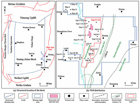
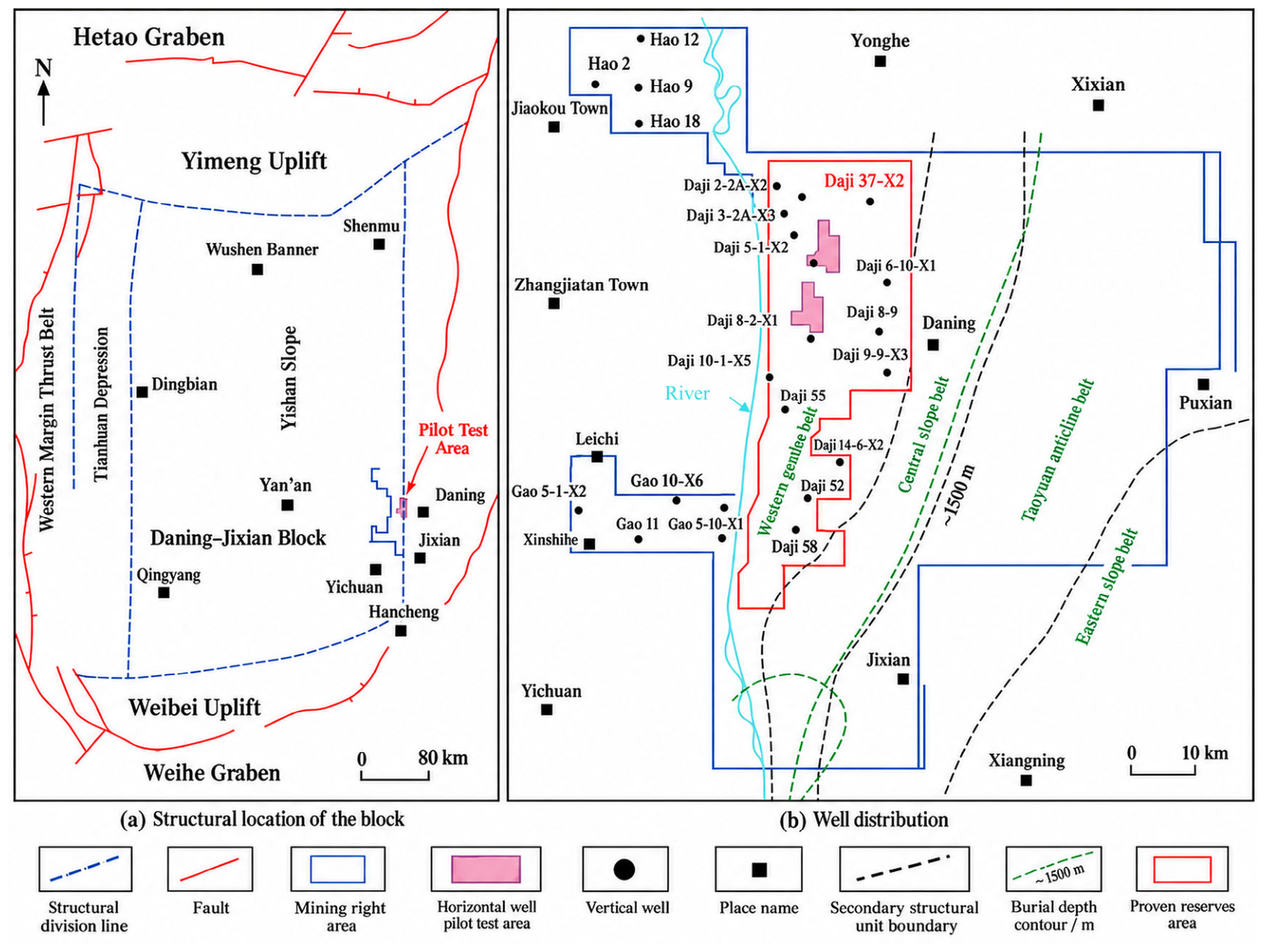
The study area lies in the Daning–Jixian Block on the eastern margin of the Ordos Basin (Figure 1). The primary target is Coal Seam No. 8, and the studied intervals are generally deeper than 2000 m. The seam is laterally continuous and mainly consists of primary-structure coal. The reservoir is characterised by high in situ stress and low permeability. Spatial variations in natural fractures, structure, coal mechanical properties, and stress create different disturbance-propagation conditions among wells. Development mainly uses multistage, multicluster fracturing of horizontal wells on multiwell pads, providing an appropriate setting for relation-level interference analysis.

Figure 1. Structural location and well distribution in the Daning–Jixian Block [3].

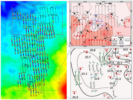
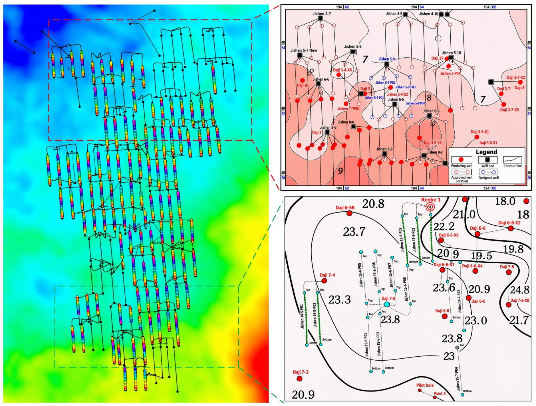
The study dataset comprises 131 horizontal wells with trajectory, fracturing and offset-well monitoring records from 2023 to 2024. It includes 39 treatment wells and 92 offset wells, covering wells with and without recorded frac-hit responses (Figure 2). Wells are arranged in multiwell pads, with locally close spacing and interspersed treatment and offset wells. The data comprise geology and in situ stress, well trajectories and spatial relations, treatment parameters, offset-well states, and dynamic monitoring records.

Figure 2. Spatial distribution of study wells and representative local well-pattern characteristics in the Daning–Jixian Block. Red and green dashed boxes and guide lines locate the areas enlarged in the upper-right and lower-right views, respectively. Well symbols in the upper-right inset are defined in its legend.

2.2. Frac-Hit Identification and Relation-Sample Construction

Interwell interference is represented as a directed relation from a treatment stage to an offset well. A stage can be associated with several offset wells, and an offset well can be associated with several stages. Each stage–offset-well pair is a prediction target, with predictors restricted to information available before the target stage starts.

The recorded stage–offset-well relations were represented using three-dimensional well trajectories and target-seam correspondence. Let Γ_i denote the treatment-stage trajectory and Γ_j the offset-well horizontal trajectory within the target seam. Their minimum three-dimensional distance is

$$d_{\mathit{ij}}=\underset{x\in {\mathsf{\Gamma }}_i,y\in {\mathsf{\Gamma }}_j}{\min }{∥x-y∥}_2$$

(1)

Pairs satisfying the 1000 m distance criterion and the target-seam matching condition form the candidate set:

E_c = {(s_i, w_j), ∣d_ij ≤ 1000 m  M_ij = 1}

(2)

where M_ij indicates target-seam correspondence. The 1000 m search domain is applied within the study-well set, allowing each stage to be paired with multiple offset wells and each offset well with multiple stages. The farthest recorded frac-hit distance in the block is 950 m, whereas the designed well spacing is approximately 300 m. The 1000 m search distance therefore includes rare long-range interactions beyond the conventional well-spacing scale.

Candidate relations are defined for stage–offset-well pairs, with their nearest spatial positions characterising the local connection. Relations between different pads are included when they satisfy the distance and target-seam conditions.

Field frac-hit events were confirmed from salinity, pressure and production anomalies in offset wells associated with the execution of a specific treatment stage. Labels are taken directly from the field event records, which identify the treatment well, stage and affected offset well. Recorded frac-hit relations receive label 1, and the remaining eligible candidate relations receive label 0. The labels are defined as

$$y_{\mathit{ij}}=\left\{\begin{array}{cc}1,& (s_i,w_j) \mathrm{is\; a\; recorded\; frac}\text{-}\mathrm{hit\; relation}\\ 0,& (s_i,w_j) \mathrm{is\; another\; eligible\; candidate\; relation}\end{array}\right.$$

(3)

The 39 treatment wells contain 468 stages. Within the defined study domain, the records form 1536 stage–offset-well relations. Field-confirmed frac hits correspond to 132 positive relations; the remaining 1404 candidates receive negative labels. The positive proportion is 8.59%. All 1536 relations are retained, and predictors are assembled for each (s_i, w_j) pair.

2.3. Potential-Connectivity Corridor and Input Features

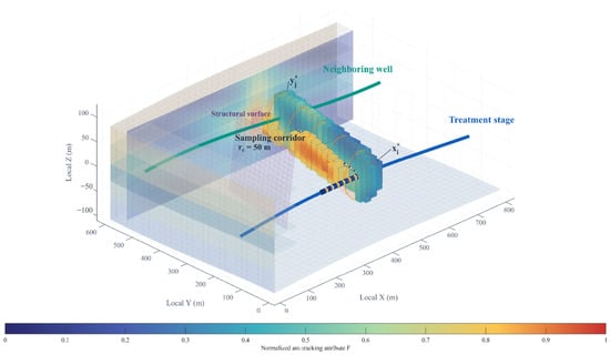
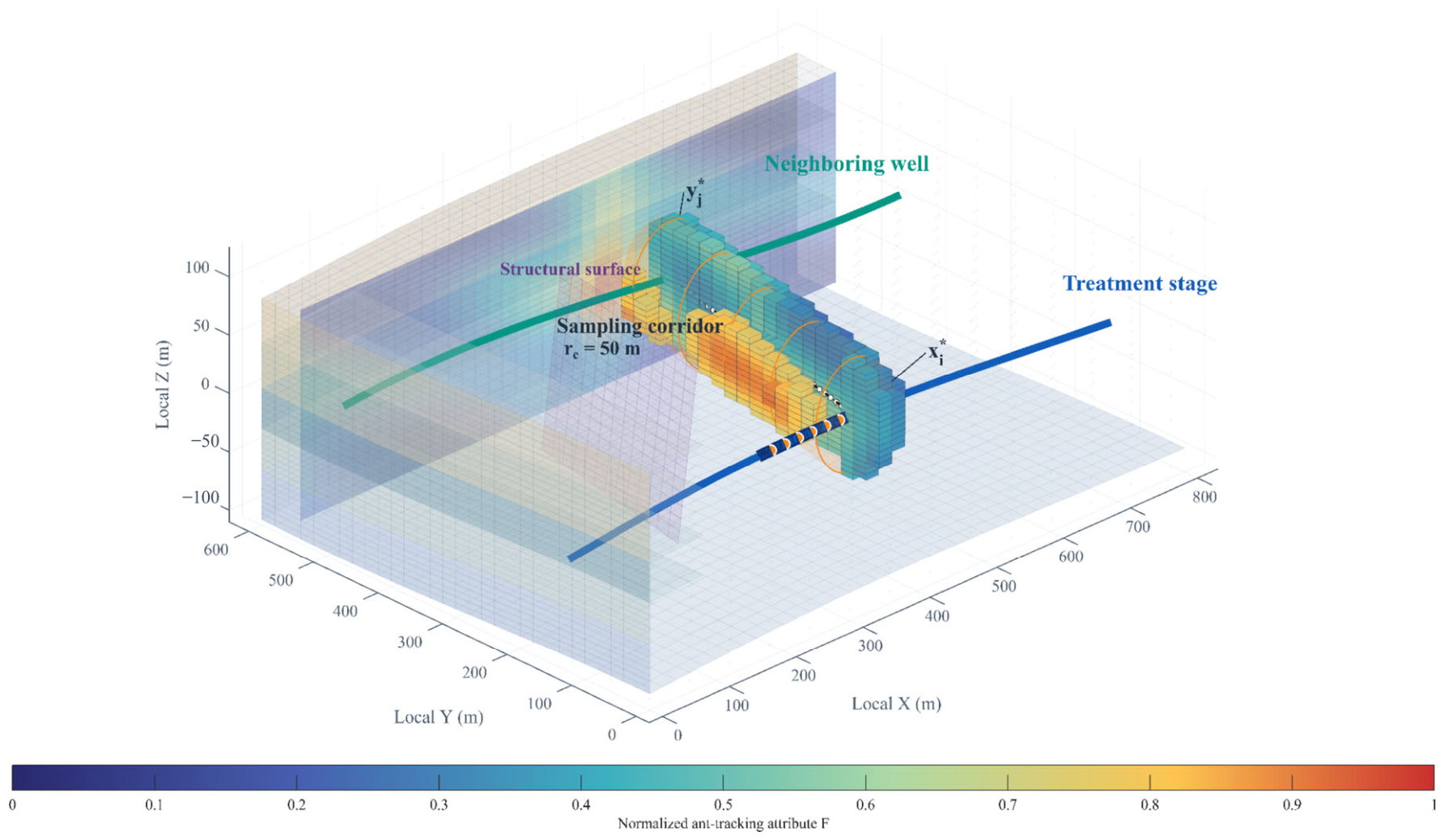
For each candidate pair, a three-dimensional potential-connectivity corridor provided a common spatial domain for sampling geological and stress attributes (Figure 3). Its axis links the treatment stage to the offset well, allowing along-path heterogeneity to be summarised consistently across pairs. The resulting corridor descriptors complement stage attributes and the pre-treatment offset-well state in the prediction model.

Figure 3. Three-dimensional potential-connectivity corridor and relation-feature sampling.

For each candidate relation, the perforation cluster, $x_i^{*}$, nearest the offset well is the start point. Its nearest point, $y_j^{*}$, on the target-seam horizontal section of the offset well is the endpoint. These points define the connecting axis, L_ij, around which a three-dimensional buffer is constructed:

C_ij = {x∣d(x, L_ij) ≤ r_c}

(4)

Here, C_ij is the sampling corridor, and r_c is its radius. The 50 m radius provides a local sampling buffer around the interwell bearing. It spans several cells of the geological grid, while field microseismic monitoring indicated fracture heights of approximately 30–40 m. This scale provides context for sampling nearby geological and stress variations. The radius was selected by grouped cross-validation within the training data and then held fixed for validation and testing.

The corridor was intersected with three-dimensional geological, seismic ant-tracking, structural, and in situ stress models. Attributes were extracted on a 20 m × 20 m × 5 m grid and sampled at 10 m intervals along the axis. Continuous attributes were obtained by trilinear interpolation, and structural crossings were identified from spatial intersections. High ant-tracking values represented fracture or structural anomalies. Corridor statistics were calculated from valid cells, with missing predictors imputed using training-subset medians. The fitted imputation and scaling parameters were then applied to the evaluation data.

(1)

Potential-connectivity features

Potential-connectivity features describe anomaly development, along-path continuity, and directional matching within a corridor. Let F(x) denote the normalised ant-tracking attribute. An anomaly threshold, F_th, is defined as the 75th percentile of the training-corridor distribution. Valid grid cells satisfying the following condition are classified as fracture-anomaly cells:

F(x) > F_th

(5)

The fraction of fracture-anomaly cells in a corridor is defined as

$$F_a={\displaystyle \frac{N_f}{N}}$$

(6)

where N_f is the number of anomalous grid cells, and N is the total number of valid cells. Invalid or missing cells are excluded from the denominator.

Continuous anomalous intervals are identified along the connecting axis, and the longest interval divided by the axis length is defined as

$$F_l={\displaystyle \frac{L_f}{{\mathcal{l}}_{\mathit{ij}}}}$$

(7)

where L_f is the length of the longest continuous anomalous interval, and 𝓁_ij is the connecting-axis length. F_l quantifies along-path seismic-anomaly continuity.

Fracture azimuth and interwell-bearing azimuth are treated with 180° periodicity. Their difference is first mapped to [0°, 180°), and the undirected acute angle is then calculated as

d_f = |θ_f − θ_ij| mod 180°, Δθ_f = min(d_f,180°−d_f)

(8)

where θ_f is the dominant fracture azimuth in the corridor, and θ_ij is the bearing from the treatment stage to the offset well. The corresponding match is defined as

F_θ = cosΔθ_f

(9)

F_θ ranges from 0 to 1, with values nearer 1 indicating stronger undirected alignment. The number of fault or structural-weakness crossings is included as an additional variable.

(2)

In situ stress-matching features

The in situ stress features describe local stress contrasts and stress variation along the interwell direction. The maximum and minimum horizontal principal stresses are σ_H and σ_h, respectively. Their difference is

Δσ_h = σ_H − σ_h

(10)

The maximum-horizontal-stress azimuth, θ_H, is treated with the same 180° periodicity. Its equivalent angle to the interwell direction is defined as

d_H = |θ_H − θ_ij| mod 180°, Δθ_H = min(d_H,180°−d_H)

(11)

The corresponding stress-direction match is defined as

S_θ = cosΔθ_H

(12)

To describe the along-path stress trend, minimum horizontal principal stress, σ_h,k, in corridor cells is linearly fitted against projected position, l_k, along the connecting axis:

σ_h,k = a + G_σl_k + ε_k

(13)

where G_σ is the minimum-horizontal-stress gradient from the treatment stage towards the offset well, a is the intercept, and ε_k is the residual. The sign of G_σ indicates whether stress generally increases or decreases in that direction.

(3)

Spatial-relation features

Spatial predictors comprise the minimum three-dimensional distance and the horizontal and vertical separations of the corresponding nearest-point pair. Directional relationships are expressed by fracture- and stress-direction matches, Fθ and Sθ. The candidate distance is calculated from the complete stage trajectory, whereas the corridor axis starts at the nearest perforation cluster. These measures describe, respectively, pair eligibility and the reference geometry for feature sampling.

(4)

Treatment features

Treatment features comprise stage length, perforation-cluster count, pumping rate, fluid-volume intensity, and proppant-mass intensity. To reduce the influence of stage length on total-volume measures, we define

$$I_{f,i}={\displaystyle \frac{V_i}{L_i}},I_{p,i}={\displaystyle \frac{M_i}{L_i}}$$

(14)

where V_i is stage fluid volume, M_i is stage proppant mass, and L_i is stage length. Local depth, coal thickness, mechanical properties, and stress provide the geological background of a stage. RF-RFE determines whether these variables enter the final predictor set. When the stage subscript is omitted, the two intensity measures are denoted by I_f and I_p.

Volume-based proppant records are expressed as equivalent mass using M = ρbVp, where Vp is bulk proppant volume, and ρb = 1.60 t m⁻³ is the bulk-density conversion factor. Fluid-volume intensity, proppant-mass intensity, and proppant loading are expressed consistently in m³ m⁻¹, t m⁻¹, and t m⁻³, respectively.

(5)

Offset-well-state features

Candidate offset-well-state variables include producing or shut-in status, production duration, cumulative gas production, and pressure depletion. Each uses the latest record before the corresponding stage begins. Pressure depletion is calculated from initial reservoir pressure and contemporaneous bottom-hole pressure:

$$\Delta P_{\mathit{ij}}=P_{0,j}-P_j\left(t_i^s\right)$$

(15)

where P_0,j is the initial reservoir pressure, and P_j(t_i^s) is the offset-well bottom-hole pressure before the stage begins, both referenced to the same depth datum. Pressure depletion and operating status are assigned to the relation edge so that the state of an offset well can vary among treatment stages.

The relation-level input combines stage attributes, basic offset-well attributes, and relation-edge attributes:

$$X_{\mathit{ij}}=\left(X_i^s,X_j^w,X_{\mathit{ij}}^r\right)$$

(16)

Here, the three terms describe stage-node, offset-well-node, and relation-edge attributes. Relation features combine geometry, corridor properties, stress matching, and the offset-well state at the start of treatment. The graph representation of these attributes is defined in Section 3.3.

The initial set contains 25 variables. Spatial and connectivity variables comprise minimum three-dimensional, horizontal, and vertical distances; F_a, F_l, and F_θ; structural-crossing count; and σ_h and σ_H. Stress and treatment variables comprise Δσ_h, S_θ, G_σ, stage length, perforation-cluster count, I_f, I_p, and Q. Reservoir and offset-well variables comprise depth, coal thickness, Young’s modulus, Poisson’s ratio, pressure depletion, operating status, production duration, and cumulative gas production.

Candidate predictors were included according to data availability, calculability and availability before treatment. Spatial distances were calculated from well trajectories. Corridor anomaly abundance, continuity and directional matching were derived from seismic ant-tracking attributes and spatial sampling. Stress differences and pathwise gradients were extracted from the stress model, while treatment intensities and offset-well states came from treatment designs, production and pressure records. Correlation analysis and subsequent screening used these extracted relation-level variables, following Section 3.2. Appendix A, Table A1, lists all 25 candidates, their units and retention status.

3. Methods

3.1. Overall Analytical Framework

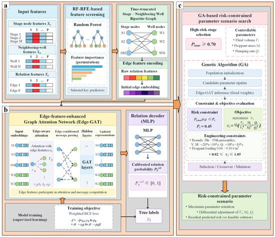
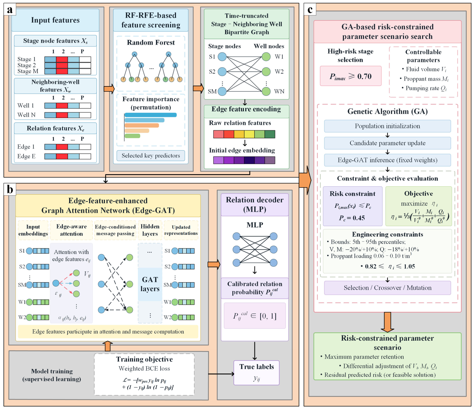
The framework combines feature construction and selection, graph-based probability prediction, and risk-constrained treatment design (Figure 4). Geological and engineering information is represented for each treatment-stage–offset-well pair. Prediction and design adjustments are evaluated using historical records and subsequent field applications.

Figure 4. Workflow for relation-level interference prediction and risk-constrained treatment design. (a) Feature screening and graph construction from stage, offset-well, and relation inputs. RF-RFE selects predictors, and the bipartite graph is reconstructed at each stage start time. (b) Edge-GAT training and prediction. Relation attributes inform attention weights and messages; an MLP decoder estimates relation probabilities, which are calibrated using validation data. The training block shows the per-relation weighted loss; Equation (29) defines its average over training relations. (c) GA-based parameter search. With model weights fixed, the GA updates fluid volume, proppant mass, and pumping rate to maximise treatment retention subject to risk and engineering constraints. Blue and green circles represent stage and offset-well nodes, respectively. Solid graph links denote candidate relations, and dashed arrows denote message passing. Orange arrows connect the principal modules; black arrows show the processing flow. Other colours distinguish schematic modules, feature components and neighbour contributions.

RF-RFE first selects predictors from the relation-level feature vectors. The retained variables are assigned to stage nodes and relation edges according to their physical meaning, while static offset-well attributes and candidate-pair connectivity provide the graph context. Edge-GAT then estimates pairwise frac-hit probabilities on a bipartite graph reconstructed at each target-stage start time. Validation data determine the probability calibration and classification threshold.

The calibrated model supplies the objective evaluations for the GA search. Fluid volume, proppant mass, and pumping rate are adjusted within engineering bounds, with geology, geometry, and pre-treatment offset-well conditions held fixed. The search seeks the greatest retention of stimulation inputs among designs satisfying the prescribed relation-risk constraint.

3.2. Variable Screening and Predictive-Contribution Analysis

RF-RFE was used to obtain a compact predictor set from 25 candidates [19,20]. The RF screening model evaluated relation-level feature vectors using cross-validated area under the precision–recall curve (PR-AUC). Permutation importance and TreeSHAP described the contributions and nonlinear responses of retained predictors [21].

Feature selection was performed within the training spatial units. Candidate variation and Spearman correlations were examined to identify data-quality issues and redundant information. Five-fold grouped cross-validation kept the nodes and relations of each spatial unit together. Each RF contained 500 trees and used balanced class weights, with the remaining hyperparameters selected within the training data.

At each recursive step, the RF was refitted to the current predictor subset and evaluated on the held-out spatial folds. Each predictor was permuted 20 times, and its importance was measured by the mean decrease in PR-AUC. The predictor with the lowest contribution was removed before the next fit. Subset size was chosen by the one-standard-error rule: the smallest subset whose mean five-fold PR-AUC was within one standard error of the best mean was retained. The standard error was calculated across the five folds as SE = SDfold/√5.

TreeSHAP values were calculated for the held-out spatial units using their corresponding fold models and then pooled across folds. The resulting distributions characterised the relationship between predictor values and RF output.

The selected subset contained 12 predictors. The other 13 candidates comprised horizontal and vertical separation, structural-crossing count, minimum and maximum horizontal principal stresses, stage length, perforation-cluster count, depth, coal thickness, Young’s modulus, Poisson’s ratio, production duration, and cumulative gas production. The 12 screened predictors populate the stage and relation attributes, complemented by offset-well geometry and graph topology.

Several excluded variables describe conditions also represented by retained predictors. Horizontal and vertical separations are components of three-dimensional distance; principal stress magnitudes contribute to stress contrast; and stage length enters the treatment-intensity definitions. Production duration and cumulative production describe well history, whereas pressure depletion and operating status describe the state immediately before treatment. The selected set emphasises these relation-specific summaries. Retention was determined by grouped predictive performance and permutation importance.

3.3. Spatial Units and Stage–Offset-Well Bipartite Graphs

Spatial units provide the common grouping for graph construction and dataset partitioning. Each unit contains treatment wells, their stages, offset wells and the associated candidate relations.

The 131 study wells were initially grouped by field well pads and operational well groups. Unique physical well identifiers were used throughout, with all stages of a treatment well kept together. Stage–offset-well candidates were established using the distance limit of 1000 m and target-seam correspondence defined in Section 2.2.

Initial groups sharing a study well or linked by a cross-group candidate relation were merged. This procedure was repeated along connected groups until separate units shared neither wells nor candidate relations. Overlapping search domains alone did not determine unit membership.

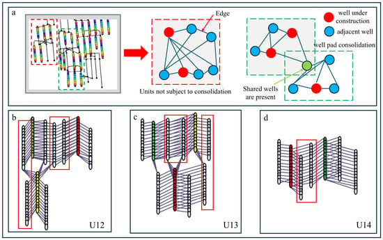
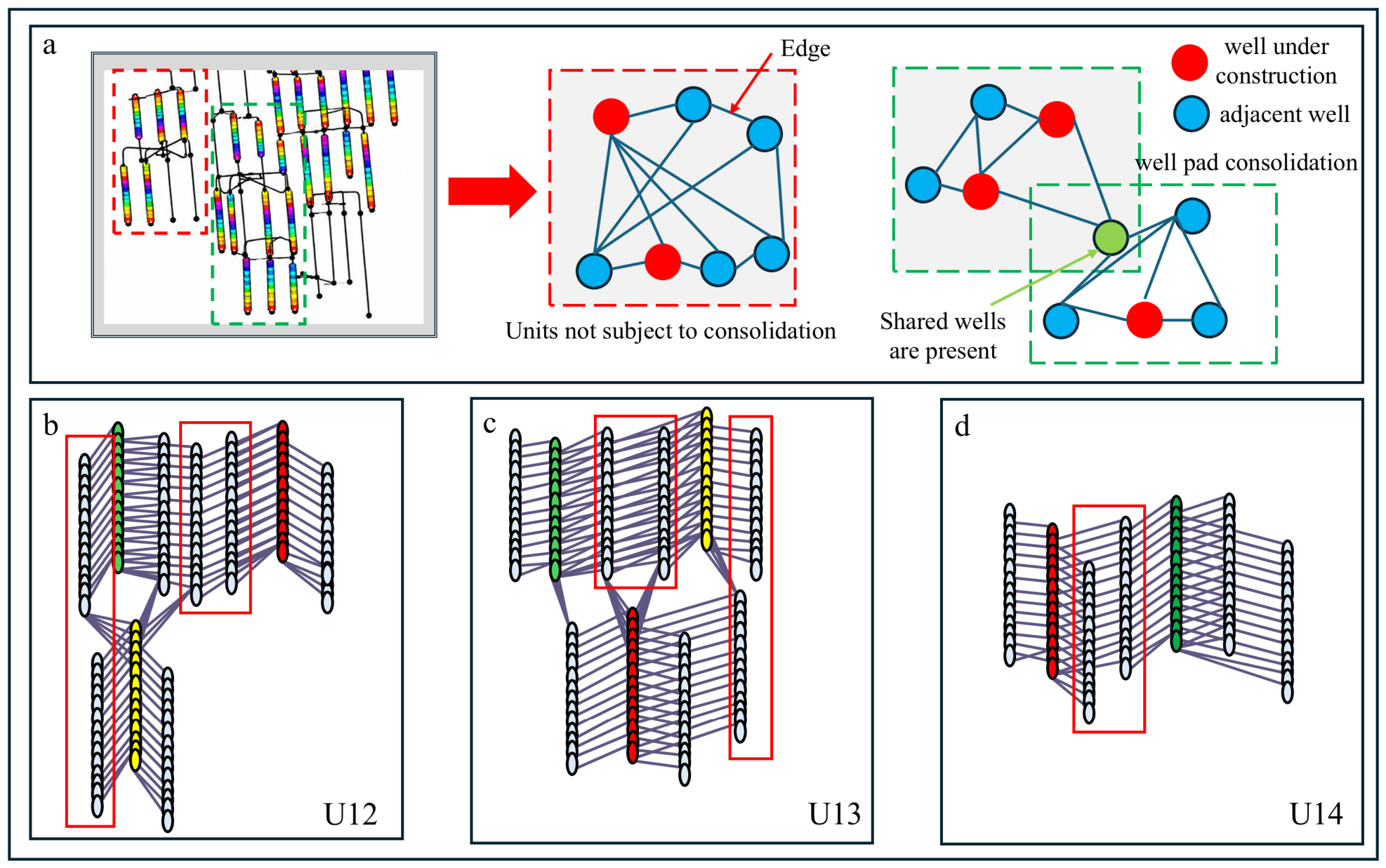
The resulting 14 units are labelled U01–U14. Table 1 lists their constituent well pads, sample counts and dataset assignments. Each unit was assigned in full to training, validation or testing, keeping its wells, stages and relations together. Figure 5 illustrates unit construction and the relation representations for U12–U14.

Table 1. Spatial-unit composition and dataset partition.

Unit	Dataset	Well Pads	Treatment Wells	Offset Wells	Stages	Relations	Positive	Negative
U01	Training	DJ1-2, DJ1-3	3	4	36	144	4	140
U02	Training	DJ2-1, DJ2-2, DJ2-3, DJ3-1	5	10	60	199	16	183
U03	Training	DJ3-2, DJ3-3, DJ3-4, DJ3-5	5	10	60	199	16	183
U04	Training	DJ4-1, DJ4-2	2	5	22	56	11	45
U05	Training	DJ5-3, DJ5-4, DJ5-5	3	7	33	100	8	92
U06	Training	DJ6-1, DJ6-2, DJ6-3	2	6	22	100	8	92
U07	Training	DJ6-4, DJ6-5	2	7	23	100	8	92
U08	Training	DJ7-1, DJ7-2	2	7	22	100	8	92
U09	Validation	DJ7-3, DJ8-2, DJ8-3	3	7	37	119	11	108
U10	Validation	DJ9-1, DJ9-2	2	5	26	75	8	67
U11	Validation	DJ10-2, DJ10-3	2	5	26	75	7	68
U12	Test	DJ11-1, DJ11-2, DJ11-3	3	7	38	107	11	96
U13	Test	DJ12-2, DJ12-3, DJ12-4	3	7	37	104	10	94
U14	Test	DJ13-1, DJ13-2	2	5	26	58	6	52
Total	All datasets	37	39	92	468	1536	132	1404

Figure 5. Spatial-unit construction and the mapping of stage–offset-well relations. (a) Schematic of unit construction; (b–d) schematic relation representations for units U12, U13 and U14, respectively. Coloured point sequences indicate treatment stages, white point sequences indicate offset wells, and solid lines indicate neighbouring connections.

A complete spatial unit defines the graph-construction domain. The graph for unit k is defined as

$$G_k=\left(V_s^k,V_w^k,E_c^k\right),$$

(17)

where $V_s^k$ and $V_w^k$ are the treatment-stage and offset-well node sets, respectively, and $E_c^k$ contains the candidate pairs meeting the distance and target-seam criteria.

Stage-node attributes, $X_i^s$, primarily describe geological and engineering properties of a stage, including fluid-volume intensity, proppant-mass intensity, pumping rate, and local horizontal stress difference. Offset-well-node attributes, $X_j^w$, encode trajectory geometry and target-seam position. Time-varying offset-well operating status and pressure depletion join spatial, corridor, and stress-matching variables as relation-edge attributes:

$$X_{\mathit{ij}}^r=\left[d_{\mathit{ij}},F_a,F_l,F_{\theta },S_{\theta },G_{\sigma },\Delta P_{\mathit{ij}},S_{\mathit{ij}}^p\right],$$

(18)

where d_ij is the minimum three-dimensional distance; F_a and F_l describe anomaly abundance and continuity; F_θ and S_θ describe directional matching; G_σ is the stress gradient; and ΔP_ij and $S_{\mathit{ij}}^p$ describe the pre-treatment offset-well state. For each target stage, s_i, the graph includes the stages, candidate relations, and dynamic states available at its start time, together with the target stage’s design parameters. Later stages are masked. The resulting temporally truncated graph is denoted G_k.

Frac-hit prediction was formulated as binary classification on candidate edges, using the labels defined in Equation (3). For a treatment stage, s_i, and offset well, w_j, the network estimates the uncalibrated probability

$${\widehat{P}}_{\mathit{ij}}=P\left(y_{\mathit{ij}}=1\mid G_k,X_i^s,X_j^w,X_{\mathit{ij}}^r\right),$$

(19)

where G_k supplies the topological context of the surrounding stages and offset wells.

3.4. Edge-Enhanced Graph Attention Network

Edge-GAT uses neural message passing to update entity representations by transforming and aggregating neighbourhood information [22]. The two node types and relation edges are encoded separately. Edge attributes participate in both attention weights and message construction, and the relation classifier combines the learned endpoint and edge representations.

The initial representations of stages, offset wells, and relation edges are

$$h_i^{s,\left(0\right)}={\varphi }_s\left(X_i^s\right); h_j^{w,\left(0\right)}={\varphi }_w\left(X_j^w\right); h_{\mathit{ij}}^e={\varphi }_e\left(X_{\mathit{ij}}^r\right)$$

(20)

where φ_s, φ_w, and φ_e are independent encoders that map source-specific attributes into a common latent space. Superscripts s and w denote stage and offset-well nodes, and superscript e denotes encoded relation attributes.

At graph layer l, the attention score between stage s_i and offset well w_j is defined as

$$e_{\mathit{ij}}^{\left(l\right)}=\mathrm{LeakyReLU}\left\{a^{\left(l\right)\mathrm{T}}\left[W_s^{\left(l\right)}{h}_i^{s,\left(l\right)}\parallel W_w^{\left(l\right)}{h}_j^{w,\left(l\right)}\parallel W_e^{\left(l\right)}{h}_{\mathit{ij}}^e\right]\right\}$$

(21)

where ‖ denotes concatenation, and W_s, W_w, W_e, and a are learnable parameters. Adjacent stages are normalised for each offset well:

$${\alpha }_{\mathit{ij}}^{s\to w,\left(l\right)}={\displaystyle \frac{\exp \left(e_{\mathit{ij}}^{\left(l\right)}\right)}{\sum _{r\in {\mathcal{N}}_s\left(j\right)}\exp \left(e_{\mathit{rj}}^{\left(l\right)}\right)}}$$

(22)

N_s(j) denotes the stages linked to offset well w_j. The attention weights depend on the endpoint features and the attributes of their connecting relation.

The edge-conditioned message from a stage to an offset well is

$$m_{\mathit{ij}}^{s\to w,\left(l\right)}=W_{\mathit{sw}}^{\left(l\right)}{h}_i^{s,\left(l\right)}+U_{\mathit{sw}}^{\left(l\right)}{h}_{\mathit{ij}}^e$$

(23)

The offset well aggregates messages from its adjacent stages:

$${\tilde{h}}_j^{w,\left(l+1\right)}=\psi \left(\sum _{i\in {\mathcal{N}}_s\left(j\right)}{\alpha }_{\mathit{ij}}^{s\to w,\left(l\right)}{m}_{\mathit{ij}}^{s\to w,\left(l\right)}\right)$$

(24)

where ψ is a nonlinear activation function. A residual connection then updates the aggregated representation:

$$h_j^{w,l+1}={\tilde{h}}_j^{w,l+1}+W_{\mathit{res},w}^l{h}_j^{w,l}$$

(25)

A learnable projection aligns the residual and updated dimensions. Stage nodes aggregate offset-well information using the same structure with independent transformations in the reverse direction. Multihead outputs are combined and linearly projected before the next layer; the hidden dimension in Table 2 is the resulting layer-output dimension.

Table 2. Edge-GAT hyperparameter ranges and selected configuration.

Parameter	Search Range	Selected Value
Edge-GAT layers	1, 2, 3	2
Hidden dimension	32, 64, 128	64
Attention heads	2, 4, 8	4
Dropout rate	0.10, 0.20, 0.30	0.20
Optimiser	Adam, AdamW	AdamW
Initial learning rate	10−4, 5×10−4, 10−3	10−3
Weight decay	10−5, 10−4, 10−3	10−4
Maximum epochs	—	500
Early-stopping patience	20, 30, 40	30

After L graph layers, the representations of both endpoint nodes and their relation edge are concatenated to form the edge-classification representation:

$$z_{\mathit{ij}}=\left[h_i^{s,\left(L\right)}\parallel h_j^{w,\left(L\right)}\parallel h_{\mathit{ij}}^e\right]$$

(26)

The edge classifier then outputs a probability:

$$u_{\mathit{ij}}={\mathrm{MLP}}_{\mathit{dec}}\left(z_{\mathit{ij}}\right),P_{\mathit{ij}}={\displaystyle \frac{1}{1+\exp (-u_{\mathit{ij}})}}$$

(27)

In Equations (26) and (27), z_ij is the concatenated relation representation, MLP_dec produces the scalar logit, u_ij, and the sigmoid converts the logit to the uncalibrated probability, P_ij.

3.5. Training, Probability Calibration, and Performance Evaluation

The 14 spatial units were assigned in full to eight training units (U01–U08), three validation units (U09–U11) and three held-out test units (U12–U14), as shown in Table 1. These datasets contain 998 relations (79 positive and 919 negative), 269 relations (26 positive and 243 negative), and 269 relations (27 positive and 242 negative), respectively. Each study well, its stage or offset-well nodes, and its candidate relations remain within one subset [23]. Validation units are used for calibration and threshold selection; test units provide a spatially held-out evaluation within the study block.

Graphs were reconstructed at the start of each target stage within the assigned subset. Static geological and trajectory attributes were combined with the stage design and the latest available offset-well state. This grouped, time-ordered construction maintained the spatial partition and the prediction-time information boundary throughout training and evaluation.

Continuous variables are standardised using training-data statistics:

$$x^{\prime }={\displaystyle \frac{x-{\mu }_{\mathrm{tr}}}{{\sigma }_{\mathrm{tr}}}},$$

(28)

where μ_tr and σ_tr are the training mean and standard deviation. These statistics and the training-derived imputation parameters were applied to the validation and test data. Categorical predictors were encoded as binary or one-hot variables.

Every candidate relation in the training spatial units has a supervised label and contributes to the loss. Class-weighted binary cross-entropy addresses the positive–negative imbalance:

$$\mathcal{L}=-{\displaystyle \frac{1}{\mid E_{\mathrm{tr}}\mid }}\sum _{\left(i,j\right)\in E_{\mathrm{tr}}}\left[w_{+}{y}_{\mathit{ij}}\log {\widehat{P}}_{\mathit{ij}}+\left(1-y_{\mathit{ij}}\right)\log \left(1-{\widehat{P}}_{\mathit{ij}}\right)\right],$$

(29)

where E_tr is the training-relation set, y_ij is the binary relation label, and ${\widehat{P}}_{\mathit{ij}}$ is the uncalibrated Edge-GAT probability. The positive-class weight is $w_{+}={\displaystyle \frac{N_{-}}{N_{+}}}.$ For the complete training set, the ratio is

$$w_{+}={\displaystyle \frac{919}{79}}\approx 11.63.$$

Class weights are recalculated from the fitting portion of each cross-validation fold. Early stopping monitors held-out-fold PR-AUC, which focuses on positive-class performance in imbalanced datasets [24].

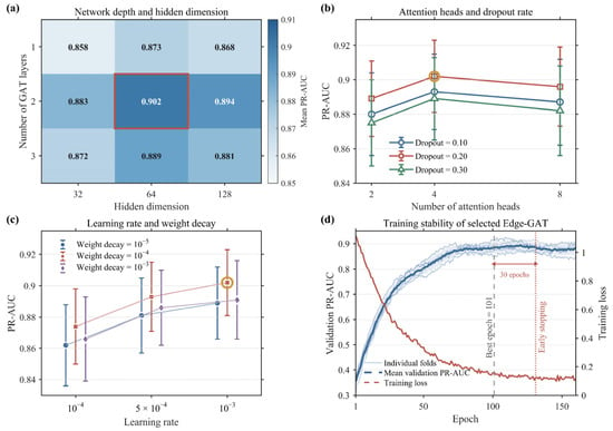
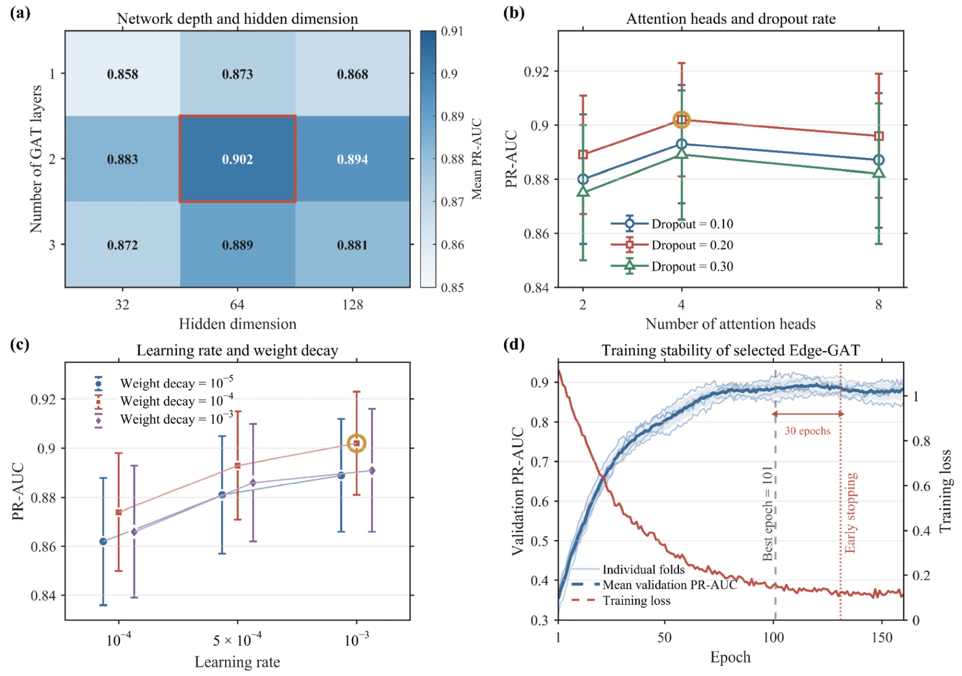
Network architecture and training hyperparameters were selected by five-fold grouped cross-validation within the eight training units. The held-out unit sets were {U01, U04}, {U05, U07}, {U06, U08}, {U02}, and {U03}. Whole units were retained in each fitting or held-out fold. PR-AUC was the primary selection metric, supplemented by area under the receiver operating characteristic curve (ROC-AUC). Figure 6 summarises the comparisons and training behaviour, and Table 2 lists the search ranges and selected values.

Figure 6. Cross-validation selection of key Edge-GAT hyperparameters and training stability. (a) Mean PR-AUC for combinations of network depth and hidden dimension; the red rectangle marks the selected combination. (b) Attention-head and dropout-rate comparison. (c) Learning-rate and weight-decay comparison. Error bars in (b,c) represent between-fold standard deviations, and gold circles identify the selected settings. (d) Training stability: pale blue curves show individual folds, the dark blue dashed curve shows mean validation PR-AUC, and the red curve shows training loss. The grey dashed and red dotted vertical lines mark the best epoch and early stopping, respectively; the double-headed arrow indicates the 30-epoch patience interval.

The selected model contains two graph layers, 64-dimensional hidden representations, four attention heads and a dropout rate of 0.20 (Figure 6a,b). The learning rate and weight decay are 10⁻³ and 10⁻⁴, respectively (Figure 6c).

Validation PR-AUC stabilised after approximately 100 epochs (Figure 6d). The median best epoch across folds was 101, with an early-stopping patience of 30 epochs. The selected network was then fitted for 101 epochs using all eight training units. Its cross-validation mean PR-AUC and ROC-AUC were 0.902 ± 0.021 and 0.948 ± 0.017, respectively, where ± denotes the between-fold standard deviation.

After network training, Platt scaling was fitted to the three validation spatial units. For the classifier logit, u_ij, in Equation (27), the calibrated relation probability is

$$P_{\mathit{ij}}^{\mathrm{cal}}=\sigma \left(a{u}_{\mathit{ij}}+b\right),$$

(30)

where a and b are estimated from validation predictions and labels, and σ(⋅) is the sigmoid function. The fitted mapping is fixed during test evaluation and treatment-parameter search. Calibration is assessed using the Brier score and reliability curves [25,26].

The classification threshold is also selected only from the validation set by maximising F₁:

$${\tau }^{*}=\arg \underset{\tau }{\max }{F}_1\left(\tau \right),$$

(31)

The selected threshold, τ^* = 0.50, was then applied to the calibrated test probabilities.

The held-out test set contained 27 positive and 242 negative relations. PR-AUC, ROC-AUC, precision, recall, F1, and accuracy were calculated from predictions reconstructed at each stage start time. The proposed model, comparison models, and ablation variants used the same spatial partitions and candidate relations, with training-derived preprocessing and validation-derived calibration and classification settings.

3.6. Treatment-Parameter Scenario Search Under a Risk Constraint

The calibrated relation probabilities were used to screen stages for parameter adjustment. In this section, P_ij denotes the probability in Equation (30), and N_i is the set of candidate offset wells for stage s_i. The maximum relation probability is

$$P_i^{\max }=\underset{j\in {\mathcal{N}}_i}{\max }{P}_{\mathit{ij}}.$$

(32)

Stages with $P_i^{\max }\ge 0.70$ entered the parameter search. The decision vector contains stage fluid volume, proppant mass, and pumping rate:

x_i = (V_i, M_i, Q_i),

(33)

where V_i, M_i, and Q_i denote fluid volume, proppant mass, and pumping rate, respectively. Fluid-volume and proppant-mass intensities were updated simultaneously after adjustment:

$$I_{f,i}={\displaystyle \frac{V_i}{L_{s,i}}},I_{p,i}={\displaystyle \frac{M_i}{L_{s,i}}},$$

(34)

where L_s,i is the stage length. Geological and stress conditions, interwell geometry, the potential-connectivity corridor, and the pre-treatment offset-well state remained fixed.

The search maximised retention of the original stimulation inputs subject to a prescribed risk-control level. The validation-derived classification threshold τ^* = 0.50 served as a reference; the main search used P_c = 0.45, with 0.40 and 0.50 examined for comparison. The treatment-retention index was defined as

$${\eta }_i={\displaystyle \frac{1}{3}}\left({\displaystyle \frac{V_i}{V_i^0}}+{\displaystyle \frac{M_i}{M_i^0}}+{\displaystyle \frac{Q_i}{Q_i^0}}\right),$$

(35)

where superscript 0 denotes the original treatment parameters. Subject to

$$P_i^{\max }\left(x_i\right)\le P_c$$

(36)

The objective was to maximise treatment retention:

$$\underset{x_i}{\max }{\eta }_i\left(x_i\right).$$

(37)

The objective favours the largest retained treatment input among scenarios satisfying the risk constraint. Fluid volume, proppant mass, and pumping rate can therefore be redistributed within the feasible range.

The retention index measures relative engineering inputs. Field evaluation focused on stage-level interference, with whole-well production providing an auxiliary description of early production behaviour.

Decision-variable ranges combined training-data distributions and relative bounds around the original design:

$$x_{i,k}^L=\max \left(q_{0.05,k},{\alpha }_k{x}_{i,k}^0\right),x_{i,k}^U=\min \left(q_{0.95,k},1.10x_{i,k}^0\right),$$

(38)

Here, x_i,k ∈ {V_i, M_i, Q_i}. The quantities q_0.05,k and q_0.95,k are the 5th and 95th percentiles of the corresponding training parameters. Fluid volume and proppant mass use α_k = 0.80, whereas pumping rate uses α_k = 0.82. Their training-set 5th–95th percentile intervals are 2,200–4,200 m³, 180–360 t and 14–22 m³ min⁻¹, respectively. Any parameter may increase by at most 10% relative to the original design. The following constraint also applies:

0.82 ≤ η_i ≤ 1.05,

(39)

Proppant loading, expressed as proppant mass in tonnes per cubic metre of fluid, was constrained by

$$0.06\le {\displaystyle \frac{M_i}{V_i}}\le 0.10\mathrm{t}/{\mathrm{m}}^3,$$

(40)

This loading constraint was applied jointly with the parameter bounds and treatment-retention limits.

For each candidate design, V_i, M_i, Q_i, and their derived intensity variables were updated in the graph corresponding to stage s_i. The fitted preprocessing, Edge-GAT, and Platt mapping were then applied to obtain the offset-well relation probabilities. Their mean was calculated as

$$P_i^{\mathrm{mean}}={\displaystyle \frac{1}{\mid {\mathcal{N}}_i\mid }}{\sum }_{j\in {\mathcal{N}}_i}{P}_{\mathit{ij}},$$

(41)

The maximum and mean summarise, respectively, the highest-risk candidate pair and the average pairwise risk around the stage.

A real-coded GA [27] uses a population of 60, a maximum of 100 generations, crossover probability of 0.85, mutation probability of 0.10 and two elite individuals. A run stops when improvement in the best objective remains below 10⁻⁴ for 15 consecutive generations. Each stage is searched independently in 20 runs. Designs satisfying the parameter, proppant-loading, input-retention and $P_i^{\max }\le P_c$ constraints are ranked by η_i. When η_i differs by less than 0.01, lower mean risk and smaller parameter changes are preferred. If no design satisfies P_c, the evaluated design with the lowest maximum relation probability is retained among those satisfying the engineering constraints.

3.7. Field Application and Historical Comparison

The field comparison included six trial stages and six historical control stages in the same target formation, selected for similar geological parameters. The established model was applied before treatment of the trial stages. Original designs were evaluated, parameter adjustments were generated by the constrained search, and the changes were implemented during treatment. The trial stages were designated S02, S05, S011, S013, S020, and S022.

Recorded frac-hit events and maximum offset-well pressure responses were compared at the stage level. For the probability comparison, high-risk relations were selected from the original-design predictions and pooled across all six stages in each group. The trial group retained the same selected relations when the adjusted designs were evaluated. The pooled mean was calculated as

$$R_g^{\left(a\right)}={\displaystyle \frac{\sum _{i\in S_g}\sum _{j\in H_{g,i}}{P}_{g,\mathit{ij}}^{\left(a\right)}}{\sum _{i\in S_g}\left|H_{g,i}\right|}}.$$

(42)

Here, g denotes the trial or control group, S_g contains its six comparison stages, and H_g,i contains the offset-well relations whose original-design calibrated probabilities exceeded 0.70. Superscript a = 0 denotes the original design and a = 1 the adjusted trial design. Every selected relation contributes equally to the group mean.

Production measurements were available at the whole-well level. The treatment wells associated with trial and control stages did not overlap. Each well contributed one record to the production summaries. First-30-day mean daily gas production and first-90-day cumulative gas production were reported as auxiliary indicators of early whole-well performance.

4. Results

4.1. Key Predictors and Nonlinear Responses

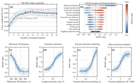
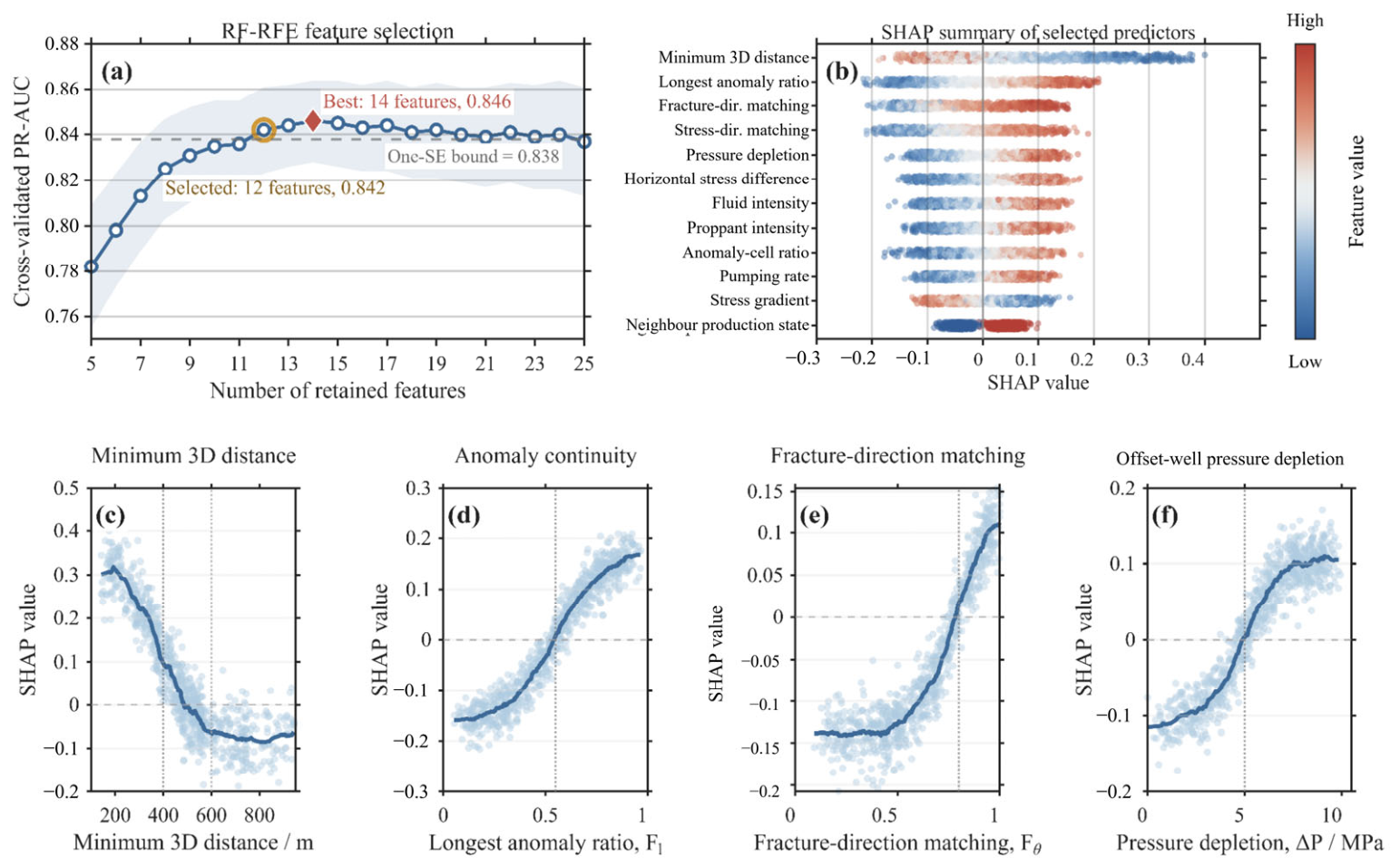
RF-RFE achieved its highest five-fold mean PR-AUC of 0.846 with 14 predictors (Figure 7a). The fold standard deviation was 0.018, giving a standard error of approximately 0.008 and a one-standard-error bound of 0.838. The 12-predictor subset scored 0.842 and was the smallest subset satisfying this criterion.

Figure 7. RF-RFE predictor selection and SHAP analysis. (a) Grouped cross-validation mean PR-AUC versus predictor count; the red diamond marks the best subset, the gold circle marks the subset selected by the one-standard-error rule, shading indicates between-fold standard deviation, and the grey dashed line indicates the one-standard-error bound. (b) SHAP distributions for the 12 retained predictors in Table 3; blue and red indicate lower and higher predictor values, respectively. (c) Minimum three-dimensional distance. (d) Longest continuous-anomaly fraction. (e) Fracture-direction matching. (f) Pre-treatment offset-well pressure depletion. In (c–f), pale points are relation-level SHAP values and dark blue curves are smoothed trends; horizontal dashed lines indicate zero SHAP contribution, and vertical dotted lines mark the reference values discussed in the text.

Minimum three-dimensional distance had the highest normalised permutation importance, followed by anomaly continuity and fracture-direction matching (Table 3). Spatial and connectivity predictors accounted for 41.9% of the selected RF model’s total importance, followed by stress (23.5%), treatment (21.2%) and offset-well state (13.4%). Figure 7b shows the corresponding SHAP distributions.

Table 3. Selected variables and normalised RF permutation importance.

Rank	Feature	Category	Normalised Permutation Importance
1	Minimum three-dimensional distance	Spatial relation	0.130
2	Longest continuous-anomaly fraction, Fl	Potential connectivity	0.116
3	Fracture-direction match, Fθ	Potential connectivity	0.105
4	Stress-direction match, Sθ	In situ stress	0.094
5	Offset-well pressure depletion, ΔPij	Offset-well status	0.087
6	Horizontal stress difference, Δσh	In situ stress	0.081
7	Fluid-volume intensity, If	Treatment parameter	0.076
8	Proppant-mass intensity, Ip	Treatment parameter	0.073
9	Anomaly-cell fraction, Fa	Potential connectivity	0.068
10	Pumping rate, Q	Treatment parameter	0.063
11	Along-path stress gradient, Gσ	In situ stress	0.060
12	Offset-well operating status	Offset-well status	0.047

Minimum three-dimensional distance was negatively associated with RF output (Figure 7c). The smoothed SHAP response was positive at short distances, decreased rapidly over approximately 300–500 m, and stabilised at negative values beyond approximately 600 m.

The longest continuous anomaly ratio showed a nonlinear response (Figure 7d). SHAP values changed from negative to positive above approximately 0.55, indicating higher RF probabilities for relations with greater anomaly continuity.

Positive SHAP contributions became more common when fracture-direction matching exceeded approximately 0.80 (Figure 7e). Relations more closely aligned with the dominant fracture direction generally received higher predicted risks.

SHAP values also increased with offset-well pressure depletion (Figure 7f). Positive contributions were concentrated mainly above approximately 5 MPa, associating greater depletion with higher RF outputs within the observed range.

4.2. Predictive Performance and Model Comparison

Comparison models included logistic regression (LR), RF, XGBoost [28], a multilayer perceptron (MLP), a graph convolutional network (GCN) [29] and a graph attention network (GAT). Tabular models received the 12 selected predictors as relation vectors. GCN and GAT included relation attributes in the final edge classifier, whereas Edge-GAT additionally used them in attention weights and message construction.

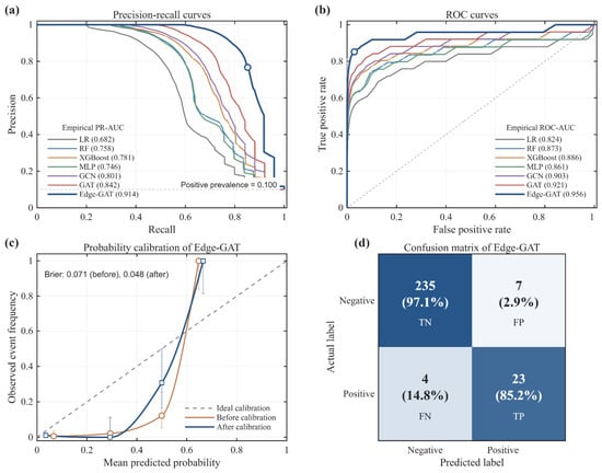
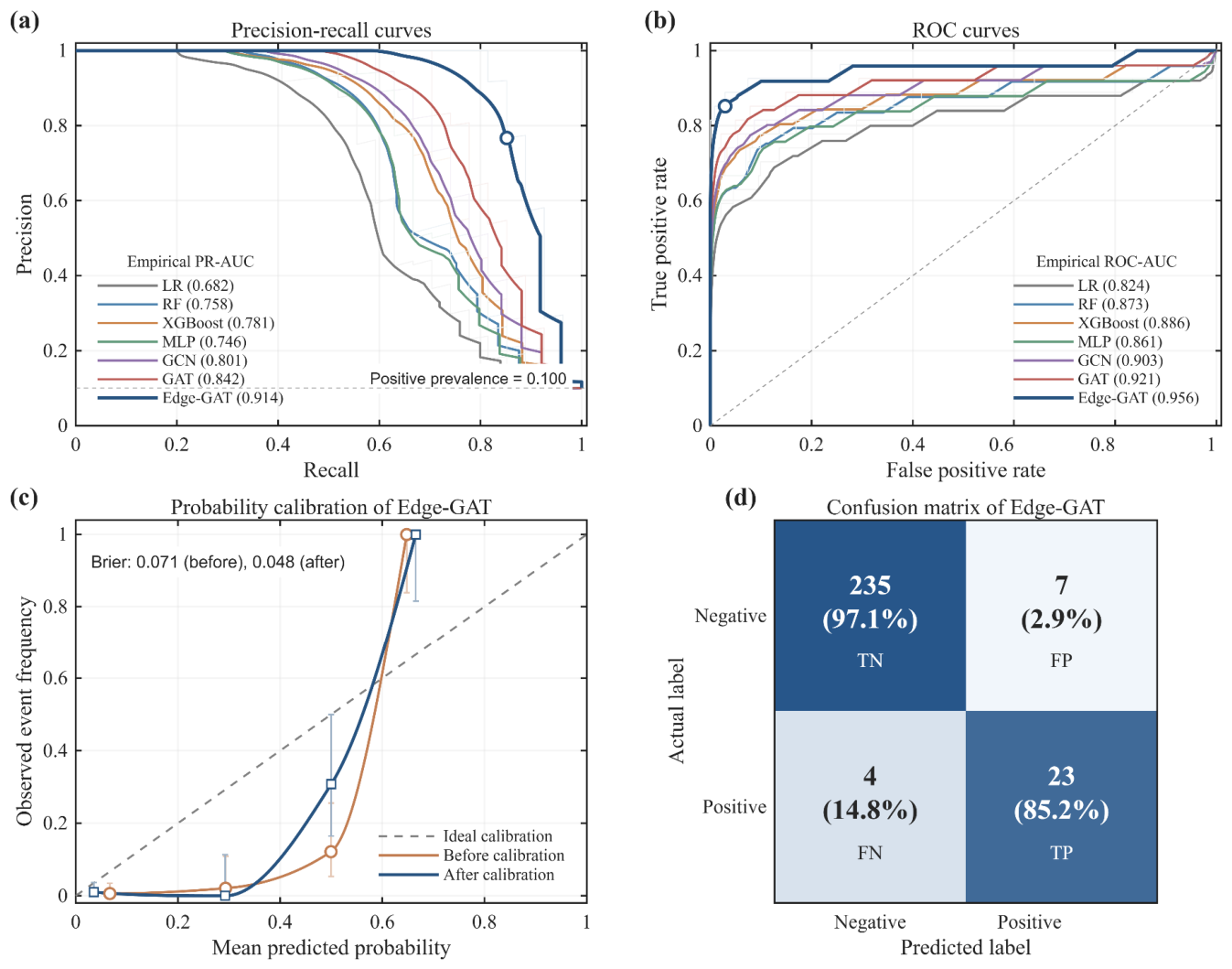
Edge-GAT achieved the highest held-out test PR-AUC and ROC-AUC, at 0.914 and 0.956, respectively (Table 4; Figure 8). Its PR-AUC exceeded GAT by 0.072 and XGBoost, the best-performing tabular model, by 0.133. Among 269 test relations, it identified 23 of 27 positives, with four false negatives and seven false positives. Precision, recall and F1 were 0.767, 0.852 and 0.807, respectively.

Table 4. Test performance of the compared models.

Model	PR-AUC	ROC-AUC	Accuracy	Precision	Recall	F1
LR	0.682	0.824	0.877	0.425	0.630	0.507
RF	0.758	0.873	0.903	0.514	0.667	0.581
XGBoost	0.781	0.886	0.914	0.556	0.741	0.635
MLP	0.746	0.861	0.900	0.500	0.667	0.571
GCN	0.801	0.903	0.926	0.606	0.741	0.667
GAT	0.842	0.921	0.937	0.656	0.778	0.712
Edge-GAT	0.914	0.956	0.959	0.767	0.852	0.807

Figure 8. Predictive performance of the comparison models and probability calibration of Edge-GAT. (a) Precision–recall curves; the horizontal dashed line indicates the positive-class prevalence in the test set. (b) Receiver operating characteristic curves; the diagonal dashed line is the chance-discrimination reference. (c) Probability calibration before and after calibration; the diagonal dashed line indicates perfect calibration. (d) Edge-GAT confusion matrix; rows indicate actual labels, columns indicate predicted labels, and percentages are calculated within each actual-label row. TN, FP, FN and TP denote true negatives, false positives, false negatives and true positives, respectively.

Applying the validation-fitted Platt mapping reduced the Brier score from 0.071 to 0.048 on the same spatially held-out test set. This improvement supports using calibrated probabilities in subsequent treatment-parameter search (Figure 8c).

Across the five training-unit validation folds, mean PR-AUC and ROC-AUC were 0.902 ± 0.021 and 0.948 ± 0.017. The corresponding held-out test values were consistent with this cross-validated performance.

4.3. Ablation and Sensitivity Analyses

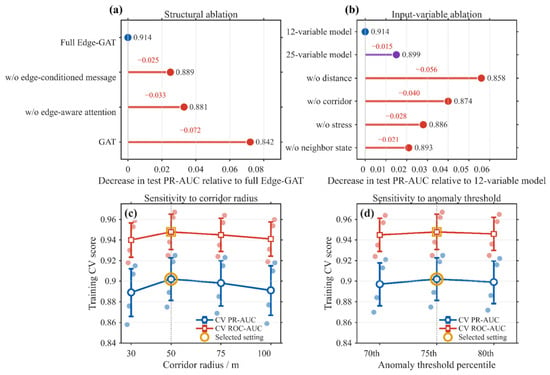
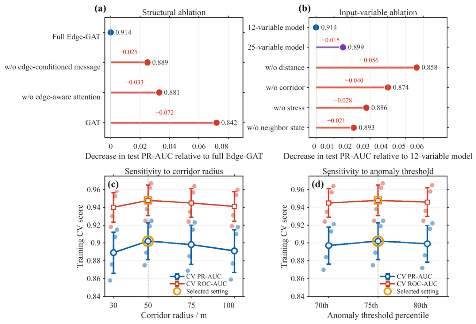
Structural and predictor ablations were evaluated on the spatially held-out test set (Figure 9a,b). Corridor radius and anomaly threshold were compared through grouped cross-validation within the training units (Figure 9c,d). The selected settings were fixed during validation and testing.

Figure 9. Edge-GAT ablation analyses and sensitivity to potential-connectivity corridor parameters. (a) Structural ablations. (b) Input-variable ablations. Horizontal displacements in (a,b) show the decrease in test PR-AUC relative to the corresponding full model; labels beside the points give the resulting PR-AUC. (c) Corridor-radius sensitivity. (d) Anomaly-threshold sensitivity. In (c,d), blue circles and red squares show mean cross-validation PR-AUC and ROC-AUC, respectively; pale points show individual-fold scores and error bars indicate between-fold standard deviations. Gold outlines and grey vertical dashed lines mark the selected settings of 50 m and the 75th percentile, respectively.

Removing edge-conditioned messages reduced PR-AUC from 0.914 to 0.889, and removing edge-enhanced attention reduced it to 0.881 (Table 5). GAT, which incorporated edge attributes only in the final classifier, achieved 0.842. Both edge-dependent attention and message content contributed to relation discrimination.

Table 5. Ablation of edge-propagation mechanisms.

Model	PR-AUC	ROC-AUC	F1
Edge-GAT	0.914	0.956	0.807
Without edge-conditioned messages	0.889	0.944	0.778
Without edge-enhanced attention	0.881	0.938	0.765
GAT	0.842	0.921	0.712

The 12-variable configuration achieved a PR-AUC of 0.914, compared with 0.899 for all 25 candidates (Table 6). Removing distance predictors reduced PR-AUC to 0.858, and removing corridor predictors reduced it to 0.874. Removal of stress and offset-well-state predictors also lowered performance, to 0.886 and 0.893, respectively. The largest decreases were associated with distance and corridor information.

Table 6. Ablation of relation-prediction variables.

Input Configuration	PR-AUC	ROC-AUC	F1
12-variable configuration	0.914	0.956	0.807
25-variable configuration	0.899	0.948	0.783
Without distance variables	0.858	0.927	0.738
Without corridor variables	0.874	0.935	0.756
Without stress variables	0.886	0.942	0.774
Without offset-well-state variables	0.893	0.947	0.783

A 50 m corridor radius achieved the highest training cross-validation mean PR-AUC of 0.902 (Figure 9c). Performance varied little over the evaluated 30–100 m range, indicating stability across these sampling widths. The 75th-percentile anomaly threshold also achieved the highest mean score, with small differences from neighbouring settings (Figure 9d).

4.4. Stage-Wise Predictions in a Representative Spatial Unit

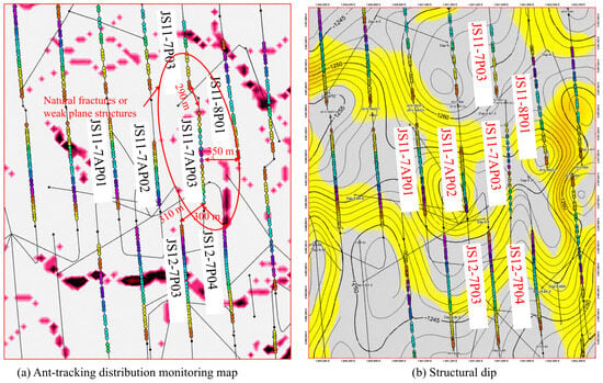
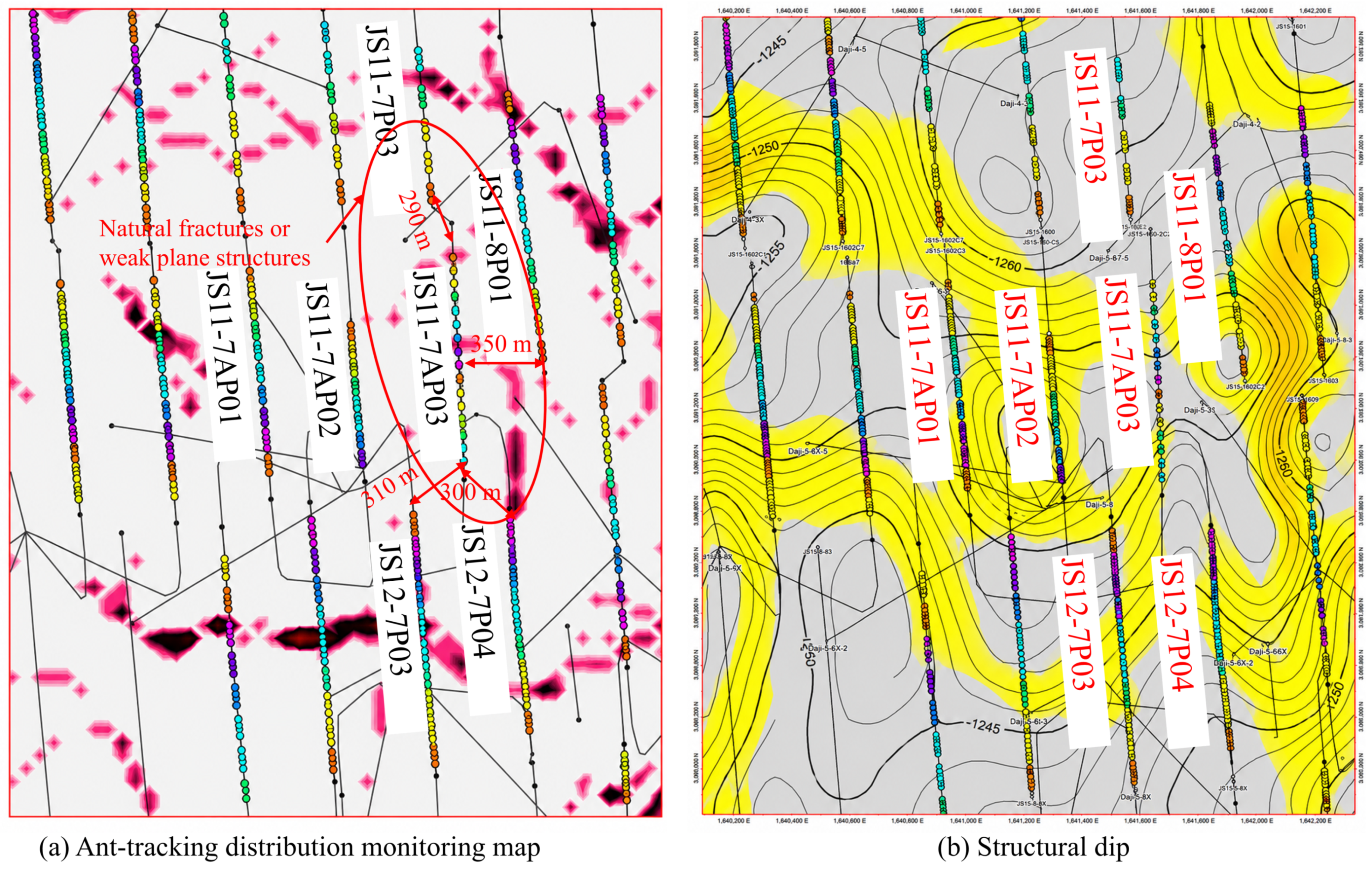
Representative training unit U01 contains treatment wells JS11-7AP01, JS11-7AP02 and JS11-7AP03, together with four offset wells. Its 36 stages form 144 candidate relations at distances of approximately 290–710 m, covering interwell and inter-row configurations. Figure 10 shows the seismic-anomaly and structural context of this well group.

Figure 10. Seismic ant-tracking anomalies and structural context of the representative spatial unit. (a) Ant-tracking anomaly distribution and interpreted natural-fracture or weak-plane features. The red ellipse highlights the local area of interwell interaction discussed in the text; red double-headed arrows indicate the labelled reference distances. (b) Structural setting of the same well group.

Four frac-hit relations were recorded during treatment of JS11-7AP03: stage 7 with JS12-7P03, stage 10 with JS11-7P03 and JS11-8P01, and stage 16 with JS12-7P04 (Table 7). Stage-wise predictions were obtained from graphs reconstructed at the respective treatment start times. Table 8 presents representative pair attributes and predicted probabilities.

Table 7. Confirmed frac-hit relations and field evidence in the representative spatial unit.

Treatment Well	Affected Offset Well	Stage	Total Stages	Reference Distance (m)	Relation Type	Principal Field Response
JS11-7AP03	JS12-7P03	7	16	310	Inter-row	Wellhead pressure, gas–water response, and salinity anomaly
JS11-7AP03	JS11-7P03	10	16	290	Inter-row	Wellhead pressure, gas–water response, and salinity anomaly
JS11-7AP03	JS11-8P01	10	16	350	Interwell	Wellhead pressure, gas–water response, and salinity anomaly
JS11-7AP03	JS12-7P04	16	16	300	Interwell	Wellhead pressure, gas–water response, and salinity anomaly

Table 8. Representative stage–offset-well attributes and Edge-GAT predictions.

Well–Stage	Offset Well	Minimum 3D Distance (m)	Fl	Fθ	Sθ	ΔP (MPa)	Offset-Well Status	If/Ip/Q	Calibrated Probability	Observed Label
JS11-7AP01-S3	JS11-7P03	690	0.23	0.42	0.46	2.4	Producing	43.1/3.88/17.7	0.21	0
JS11-7AP02-S6	JS11-7P03	420	0.36	0.55	0.58	3.5	Producing	46.2/4.14/18.4	0.34	0
JS11-7AP03-S7	JS12-7P03	310	0.71	0.88	0.84	6.2	Producing	49.7/4.66/19.3	0.89	1
JS11-7AP02-S8	JS12-7P03	360	0.34	0.51	0.54	3.1	Producing	46.9/4.23/18.6	0.33	0
JS11-7AP03-S10	JS11-7P03	290	0.79	0.94	0.90	7.2	Producing	52.3/4.98/20.1	0.94	1
JS11-7AP03-S10	JS11-8P01	350	0.68	0.85	0.81	6.6	Shut-in	52.3/4.98/20.1	0.88	1
JS11-7AP03-S14	JS12-7P04	300	0.29	0.47	0.43	2.7	Producing	44.8/3.95/17.9	0.25	0
JS11-7AP03-S16	JS12-7P04	300	0.74	0.91	0.86	6.9	Producing	50.8/4.82/19.7	0.91	1

Note: I_f, I_p, and Q denote fluid-volume intensity (m³ m⁻¹), proppant-mass intensity (t m⁻¹), and pumping rate (m³ min⁻¹), respectively.

The four recorded frac-hit relations received probabilities of 0.88–0.94, while the listed negative relations received probabilities of 0.21–0.34. Both offset wells affected during stage 10 of JS11-7AP03 received high predicted probabilities.

Stages 14 and 16 of JS11-7AP03 illustrate differences between relations at similar distances. Both are paired with JS12-7P04 at approximately 300 m, but their calibrated probabilities are 0.25 and 0.91. Stage 16 has greater anomaly continuity, stronger fracture- and stress-direction matching, and greater offset-well pressure depletion. These differences are consistent with the RF response patterns and the predictive contributions of corridor and offset-well state attributes.

4.5. Parameter-Scenario Search Results

Eight stages satisfying $P_i^{\max }\ge 0.70$ entered the constrained search. Seven attained the main control level, P_c = 0.45, while the best candidate found for S015 had a maximum relation probability of 0.48. Across all eight stages, mean maximum relation risk decreased from 0.866 to 0.449, and mean relation risk decreased from 0.498 to 0.307 (Table 9).

Table 9. Parameter scenarios under the frac-hit risk constraint.

Stage	Original Maximum Relation Risk, ${\mathit{P}}_{\mathbf{max}}^0$	Adjusted Maximum Relation Risk, ${\mathit{P}}_{\mathbf{max}}^{*}$	Original Mean Relation Risk, ${\mathit{P}}_{\mathbf{mean}}^0$	Adjusted Mean Relation Risk, ${\mathit{P}}_{\mathbf{mean}}^{*}$	Fluid-Volume Change (%)	Proppant-Mass Change (%)	Pumping-Rate Change (%)	Retention Index, η	Control Target
S02	0.91	0.44	0.520	0.305	−12.1	+3.8	−5.2	0.955	Met
S05	0.88	0.45	0.490	0.312	−8.2	+5.6	−3.0	0.981	Met
S09	0.93	0.44	0.560	0.298	−16.5	−6.0	−10.5	0.890	Met
S011	0.84	0.45	0.470	0.304	−5.5	+7.5	−1.5	1.002	Met
S013	0.79	0.44	0.430	0.287	−3.0	+6.5	+1.5	1.017	Met
S015	0.90	0.48	0.550	0.341	−18.0	−11.0	−14.0	0.857	Not met
S020	0.86	0.45	0.500	0.309	−9.0	+5.0	−4.0	0.973	Met
S022	0.82	0.44	0.460	0.296	−4.5	+7.0	−1.0	1.005	Met
Mean	0.866	0.449	0.498	0.307	−9.6	+2.3	−4.7	0.960	—

Note: superscripts 0 and * denote the original and GA-selected treatment scenarios, respectively.

The selected designs reduced fluid volume and pumping rate by averages of 9.6% and 4.7% while increasing proppant mass by 2.3%. The mean treatment-retention index was 0.960. Proppant mass increased in six scenarios, and three scenarios had retention indices of at least 1.0, showing that the search produced different combinations of the three adjustable parameters.

For S013, fluid volume decreased by 3.0%, while proppant mass and pumping rate increased by 6.5% and 1.5%. Maximum relation probability fell from 0.79 to 0.44, with a retention index of 1.017. S09 required larger reductions in fluid volume and pumping rate to reach the same risk-control level.

S015 remained above the 0.45 target after fluid volume, proppant mass, and pumping rate were reduced by 18.0%, 11.0%, and 14.0%, respectively. The lowest maximum relation probability found was 0.48; no design satisfying the 0.45 risk target was found within the specified constraints.

Tightening P_c from 0.50 to 0.40 reduced the number of stages with a design meeting the risk target from eight to five and lowered the treatment-retention index (Table 10). At P_c = 0.45, the seven feasible designs had a mean retention index of 0.975.

Table 10. Parameter-search results under different risk-control levels.

Risk-Control Level, Pc	Stages Meeting Target	Feasibility (%)	Mean Retention Index, η, of Feasible Scenarios
0.40	5/8	62.5	0.928
0.45	7/8	87.5	0.975
0.50	8/8	100.0	0.992

Across the 20 independent GA runs, the best feasible candidates were generally found after approximately 40–50 generations. Coefficients of variation for the retention index were below 2.5%.

4.6. Field Application Results

The six trial stages contributed 14 original-design relations with calibrated probabilities above 0.70. Their pooled mean probability decreased from 0.814 to 0.426 after parameter adjustment. The six historical control stages contributed 14 high-risk relations, with a pooled mean probability of 0.806 (Table 11 and Table 12). Frac hits were recorded in one trial stage and four control stages, corresponding to 16.7% and 66.7%, respectively. Median maximum offset-well pressure responses were 0.42 and 1.26 MPa.

Table 11. Stage-level interference outcomes and auxiliary whole-well production indicators for six trial and six control stages.

Metric	Trial Stages/Associated Wells	Control Stages/Associated Wells
Comparison stages	6	6
Original-design relations with probability > 0.70	14	14
Pooled mean probability: original design	0.814	0.806
Pooled mean probability: adjusted design	0.426	—
Stages with recorded frac hits	1	4
Stages with recorded frac hits (%)	16.7	66.7
Median maximum offset-well pressure response (MPa)	0.42	1.26
Whole-well 30-day mean daily gas (104 m3 d−1)	4.05	4.09
Whole-well 90-day cumulative gas (106 m3)	3.08	3.11

Table 12. Stage-pair comparison of baseline high-risk relation sets and observed interference responses.

Trial Stage	Control Stage	Baseline High-Risk Pairs (Trial/Control)	Mean Probability (Original/ Adjusted/Control)	Recorded Hit (Trial/Control)	Maximum Offset-Well Pressure (MPa; Trial/Control)
S02	C02	2/2	0.860/0.420/0.820	No/No	0.31/0.58
S05	C05	3/2	0.840/0.430/0.830	Yes/Yes	0.71/1.34
S011	C011	2/3	0.800/0.430/0.780	No/Yes	0.27/1.62
S013	C013	2/2	0.770/0.420/0.820	No/No	0.39/0.84
S020	C020	3/3	0.820/0.430/0.790	No/Yes	0.44/1.18
S022	C022	2/2	0.780/0.420/0.820	No/Yes	0.46/1.91

Whole-well production indicators showed small differences between the associated treatment wells. First-30-day mean daily gas production was 4.05 × 10⁴ m³ d⁻¹ for wells associated with the trial stages and 4.09 × 10⁴ m³ d⁻¹ for those associated with the controls. First-90-day cumulative production was 3.08 × 10⁶ and 3.11 × 10⁶ m³, respectively. Both trial-associated group means were slightly lower, by approximately 1%.

5. Discussion

5.1. Research Significance and Engineering Implications

Relation-level representation links interference direction and timing to the field well network. Distance describes stage–offset-well separation, while corridor attributes characterise the intervening geological and stress environment. Their complementary ablation contributions help explain different predicted risks at similar well spacings. This interpretation agrees with studies linking interference responses to non-uniform fracture communication and local reservoir conditions [30,31]. The representative well group further illustrates how the model distinguishes offset-well responses during a fracturing operation.

Many candidate relations share treatment stages or offset wells, making a bipartite graph suitable for this setting. Edge-GAT allows relation attributes to affect both the weights and contents of neighbourhood messages. Improvements over GAT and the structural ablations indicate that this coupling provides useful information for relation classification. Coal-reservoir fracture-network simulations also show that natural-fracture distributions influence propagation patterns [32]. Combining directional matching, stress, offset-well pressure depletion and seismic anomalies describes interference conditions more fully than an individual geometric or geological indicator.

Constrained search connects predictions to engineering choices about treatment input. The stage designs show that fluid volume, proppant mass and pumping rate can play different roles in meeting a risk target. Some stages retain or increase proppant while reducing fluid volume or pumping rate. For S015, the selected design remains above the risk target despite larger parameter reductions. Such cases require complementary measures involving treatment sequencing and offset-well management. Stimulation adequacy remains important because reducing treatment intensity may incur production costs that emerge beyond the early production period. Pressure-derived fracture area and complexity can provide complementary measures of stimulation effectiveness when interpreting these adjustments [33].

The comparison of geologically similar stages within the same formation links the implemented parameter adjustments with reduced interference responses. Fewer trial stages had recorded frac hits, and the maximum pressure responses in neighbouring wells were lower. Early whole-well production means differed by approximately 1%, with the trial-associated wells marginally lower. These production indicators combine contributions from the entire treated lateral and variations in well operation, so a small whole-well difference provides limited resolution of the contribution from an individual adjusted stage.

5.2. Limitations

The spatial test evaluates transfer between well groups within one block and contains 27 positive relations among 269 candidates. Evaluation in other geological settings remains important. Production-data deconvolution can provide complementary evidence of interwell communication [34]. Transfer to other blocks requires consistent field-event definitions and stage–offset-well attribution so that evaluation remains comparable across datasets.

The corridor represents the environment sampled for prediction using a straight reference axis. Its resolution depends on the trajectory, seismic, geological, and stress models. Structures outside the buffer and differences between the sampling geometry and the actual propagation path can affect feature representativeness. The radius comparison supports prediction stability over the evaluated widths, while uncertainty in fracture geometry and geological interpretation remains part of the model uncertainty.

The predicted improvements depend on the fitted risk surface. Searching this surface can favour combinations whose risks are underestimated. The parameter and proppant-loading bounds constrain the search, although some joint combinations may remain sparsely represented in the historical data. The six trial and six control stages were selected for geological similarity within one formation; residual differences in depletion, completion, neighbouring-well conditions, and operation can still affect the comparison. Whole-well production measurements provide early operational context, while the incremental production contribution of the adjusted stages remains unresolved.

5.3. Future Work

Further evaluation should combine prospective prediction in additional well groups with longer production follow-up. Recording the original design, recommended changes, executed parameters, and subsequent responses will allow implementation effects to be assessed alongside prediction performance. External-block testing will also help establish the range of geological and operating conditions over which the model can be transferred.

Future optimisation can incorporate joint treatment-parameter distributions and production-related objectives, balancing interference risk against fluid coverage, fracture support, and pumping-energy input. Treatment sequence, offset-well operation, shut-in, and flowback provide additional decision variables for stages near the present feasibility limits.

Physical experiments and coupled simulations can strengthen assessments of stimulation adequacy. Phase-field models of hydraulic–natural fracture interactions and deep-coal temporary-plugging simulations can examine how treatment changes affect fracture propagation [35,36]. Fracturing-fluid imbibition and gas-displacement experiments can further clarify their contributions to methane desorption and recovery [37,38]. Combining these measurements with long-term production observations would support a fuller assessment of interference control and productivity.

6. Conclusions

(1)

The proposed framework combines potential-connectivity corridors, temporally truncated stage–offset-well graphs, and Edge-GAT to predict relation-level interference risk. It integrates geological heterogeneity and directional attributes with the shared structure of the well pattern, supporting stage-specific monitoring and treatment design.

(2)

RF-RFE retained 12 of the 25 candidate predictors. Minimum three-dimensional distance, anomaly continuity, and directional matching made substantial contributions to RF prediction. The graph-model ablations confirmed the complementary predictive value of distance and corridor information.

(3)

Edge-GAT achieved held-out spatial test PR-AUC, ROC-AUC, and F1 values of 0.914, 0.956, and 0.807, respectively. Its PR-AUC exceeded GAT by 0.072, and both edge-enhanced attention and edge-conditioned messages contributed to the improvement. Validation-fitted calibration reduced the test Brier score from 0.071 to 0.048.

(4)

Constrained parameter search reduced mean maximum predicted relation risk from 0.866 to 0.449 across eight high-risk stages, with a mean treatment-retention index of 0.960. In the field comparison of six trial and six control stages within the same formation, the trial stages had fewer recorded frac hits and lower offset-well pressure responses. Early whole-well production indicators showed only small differences. The comparison supports stage-specific parameter adjustment for interference control, with production assessed at the scale of the associated treatment wells.

References

- Zhang, X.; Lai, F.; Meng, Y.; Xu, X.; Li, H.; Liu, K. Dynamic production characteristics of deep coalbed methane: A case study of Daning–Jixian Block. Energy Fuels 2024, 38, 8700–8711. [Google Scholar] [CrossRef] [Scilit]
- Yang, F.; Li, B.; Wang, K.; Wen, H.; Yang, R.; Huang, Z. Extreme massive hydraulic fracturing in deep coalbed methane horizontal wells: A case study of the Linxing Block, eastern Ordos Basin, NW China. Pet. Explor. Dev. 2024, 51, 440–452. [Google Scholar] [CrossRef] [Scilit]
- Chao, H.; Li, Z.; Zhen, H.; Guo, L.; Zhang, H. Fracturing interference behavior and mechanism of deep coalbed methane horizontal wells in the Daning–Jixian Block. Coal Sci. Technol. 2025, 53, 328–339. (In Chinese) [Google Scholar] [CrossRef]
- Chen, M.; Sun, J.; Wang, L.; Yu, L.; Tian, H.; Wang, D.; Gu, X.; Yin, Z.; Zhang, H. Analysis of the main controlling factors of intra-well frac hit between deep coalbed methane in Daning-Jixian block and research on countermeasures to prevent and control it. Coal Sci. Technol. 2025, 53, 218–225. (In Chinese) [Google Scholar] [CrossRef]
- Ren, Q.; Zhang, C.; Wu, G.; Zhang, H.; Gao, S.; Sun, Z.; Gao, Y. Hydraulic fracture initiation and propagation in deep coalbed methane reservoirs considering weak plane: CT scan testing. Gas Sci. Eng. 2024, 125, 205286. [Google Scholar] [CrossRef] [Scilit]
- Huang, S.; Liu, D.; Yao, Y.; Gan, Q.; Cai, Y.; Xu, L. Natural fractures initiation and fracture type prediction in coal reservoir under different in-situ stresses during hydraulic fracturing. J. Nat. Gas Sci. Eng. 2017, 43, 69–80. [Google Scholar] [CrossRef] [Scilit]
- Awada, A.; Santo, M.; Lougheed, D.; Xu, D.; Virues, C. Is that interference? A work flow for identifying and analyzing communication through hydraulic fractures in a multiwell pad. SPE J. 2016, 21, 1554–1566. [Google Scholar] [CrossRef] [Scilit]
- Cai, Y.; Dahi Taleghani, A. Using pressure changes in offset wells for interpreting fracture driven interactions (FDI). J. Pet. Sci. Eng. 2022, 219, 111111. [Google Scholar] [CrossRef] [Scilit]
- Ning, Y.; Jin, G.; Zhu, X.; Tura, A. Well interference and fracture geometry investigation using production and low-frequency distributed acoustic sensing data in an unconventional reservoir. SPE Reserv. Eval. Eng. 2022, 25, 509–519. [Google Scholar] [CrossRef] [Scilit]
- Marongiu-Porcu, M.; Lee, D.; Shan, D.; Morales, A. Advanced modeling of interwell-fracturing interference: An Eagle Ford shale-oil study. SPE J. 2016, 21, 1567–1582. [Google Scholar] [CrossRef] [Scilit]
- Guo, X.; Wu, K.; An, C.; Tang, J.; Killough, J. Numerical investigation of effects of subsequent parent-well injection on interwell fracturing interference using reservoir-geomechanics-fracturing modeling. SPE J. 2019, 24, 1884–1902. [Google Scholar] [CrossRef] [Scilit]
- Liu, G.; Wu, X.; Romanov, V. Unconventional wells interference: Supervised machine learning for detecting fracture hits. Appl. Sci. 2024, 14, 2927. [Google Scholar] [CrossRef] [Scilit]
- Zeng, B.; Su, Y.; Wu, J.; Tang, D.; Chen, K.; Song, Y.; Shen, C.; Huang, Y.; Du, Y.; Yu, W. Quantitative characterization and risk classification of frac hit in deep shale gas wells: A machine learning approach integrating geological and engineering factors. Processes 2025, 13, 1785. [Google Scholar] [CrossRef] [Scilit]
- Chen, Y.-T.; Zhang, D.-X.; Zhao, Q.; Liu, D.-X. Interpretable machine learning optimization (InterOpt) for operational parameters: A case study of highly-efficient shale gas development. Pet. Sci. 2023, 20, 1788–1805. [Google Scholar] [CrossRef] [Scilit]
- Zhao, G.; Yao, Y.; Wang, L.; Adenutsi, C.D.; Feng, D.; Wu, W. Optimization design of horizontal well fracture stage placement in shale gas reservoirs based on an efficient variable-fidelity surrogate model and intelligent algorithm. Energy Rep. 2022, 8, 3589–3599, Corrigendum in Energy Rep. 2022, 8, 14516. https://doi.org/10.1016/j.egyr.2022.10.431. [Google Scholar] [CrossRef] [Scilit]
- Liu, W.; Pyrcz, M.J. Physics-informed graph neural network for spatial-temporal production forecasting. Geoenergy Sci. Eng. 2023, 223, 211486. [Google Scholar] [CrossRef] [Scilit]
- Huang, Z.-Q.; Wang, Z.-X.; Hu, H.-F.; Zhang, S.-M.; Liang, Y.-X.; Guo, Q.; Yao, J. Dynamic interwell connectivity analysis of multi-layer waterflooding reservoirs based on an improved graph neural network. Pet. Sci. 2024, 21, 1062–1080. [Google Scholar] [CrossRef] [Scilit]
- Veličković, P.; Cucurull, G.; Casanova, A.; Romero, A.; Liò, P.; Bengio, Y. Graph attention networks. arXiv 2018, arXiv:1710.10903. [Google Scholar]
- Breiman, L. Random forests. Mach. Learn. 2001, 45, 5–32. [Google Scholar] [CrossRef] [Scilit]
- Guyon, I.; Weston, J.; Barnhill, S.; Vapnik, V. Gene selection for cancer classification using support vector machines. Mach. Learn. 2002, 46, 389–422. [Google Scholar] [CrossRef] [Scilit]
- Lundberg, S.M.; Lee, S.-I. A unified approach to interpreting model predictions. In Advances in Neural Information Processing Systems 30; Curran Associates, Inc.: Red Hook, NY, USA, 2017; pp. 4765–4774. [Google Scholar]
- Gilmer, J.; Schoenholz, S.S.; Riley, P.F.; Vinyals, O.; Dahl, G.E. Neural message passing for quantum chemistry. In Proceedings of the 34th International Conference on Machine Learning; PMLR: Sydney, Australia, 2017; Volume 70, pp. 1263–1272. [Google Scholar]
- Roberts, D.R.; Bahn, V.; Ciuti, S.; Boyce, M.S.; Elith, J.; Guillera-Arroita, G.; Hauenstein, S.; Lahoz-Monfort, J.J.; Schröder, B.; Thuiller, W.; et al. Cross-validation strategies for data with temporal, spatial, hierarchical, or phylogenetic structure. Ecography 2017, 40, 913–929. [Google Scholar] [CrossRef] [Scilit]
- Saito, T.; Rehmsmeier, M. The precision-recall plot is more informative than the ROC plot when evaluating binary classifiers on imbalanced datasets. PLoS ONE 2015, 10, e0118432. [Google Scholar] [CrossRef] [Scilit] [PubMed]
- Niculescu-Mizil, A.; Caruana, R. Predicting good probabilities with supervised learning. In Proceedings of the 22nd International Conference on Machine Learning, Bonn, Germany, 7–11 August 2005; pp. 625–632. [Google Scholar] [CrossRef] [Scilit]
- Brier, G.W. Verification of forecasts expressed in terms of probability. Mon. Weather Rev. 1950, 78, 1–3. [Google Scholar] [CrossRef] [Scilit]
- Whitley, D. A genetic algorithm tutorial. Stat. Comput. 1994, 4, 65–85. [Google Scholar] [CrossRef] [Scilit]
- Chen, T.; Guestrin, C. XGBoost: A scalable tree boosting system. In Proceedings of the 22nd ACM SIGKDD International Conference on Knowledge Discovery and Data Mining, San Francisco, CA, USA, 13–17 August 2016; pp. 785–794. [Google Scholar] [CrossRef] [Scilit]
- Kipf, T.N.; Welling, M. Semi-supervised classification with graph convolutional networks. arXiv 2017, arXiv:1609.02907. [Google Scholar]
- Zhang, Y.; Ge, H.; Zhao, K.; Liu, S.; Zhou, D. Simulation of pressure response resulted from non-uniform fracture network communication and its application to interwell-fracturing interference in shale oil reservoirs. Geomech. Geophys. Geo-Energy Geo-Resour. 2022, 8, 114. [Google Scholar] [CrossRef] [Scilit]
- He, Y.; He, Z.; Tang, Y.; Xu, Y.; Xu, J.; Li, J.; Sepehrnoori, K. Interwell fracturing interference evaluation in shale gas reservoirs. Geoenergy Sci. Eng. 2023, 231, 212337. [Google Scholar] [CrossRef] [Scilit]
- Zhang, L.; Chen, X.-F.; Wang, Y.; Zhang, Q.-F.; Zou, J.-P. Numerical simulation study of hydraulic fracturing network propagation in CBM development considering complex natural fracture distributions. Pet. Sci. 2026. [Google Scholar] [CrossRef] [Scilit]
- Wei, Z.; Sheng, M.; Li, J.; Zhang, B.; Wang, B.; Li, G. Pressure diagnostics in hydraulic fracturing for unconventional completion optimization. Adv. Geo-Energy Res. 2025, 17, 196–211. [Google Scholar] [CrossRef] [Scilit]
- Liu, W.-C.; Qiao, C.-C.; Wang, P.; Huang, W.-S.; Kong, X.-W.; Sun, Y.-P.; Sun, H.-D.; Jia, Y.-P. Study of inter-well interference in shale gas reservoirs by a robust production data analysis method based on deconvolution. Pet. Sci. 2024, 21, 2502–2519. [Google Scholar] [CrossRef] [Scilit]
- Yu, S.; Song, Y.; Wang, S.; Xiao, Y.; Hu, J.; Wang, Y.; Yi, L.; Yang, Z. Novel phase field model of hydraulic fracture propagation in poroelastic media and numerical investigation of interaction between hydraulic fracture and natural fracture. Petroleum 2024, 10, 672–695. [Google Scholar] [CrossRef] [Scilit]
- Pu, Y.; Li, S.; Tang, D.; Chen, S. Numerical simulation study on the effectiveness of temporary plugging and fracturing in deep coal seam to construct complex fracture network. Geoenergy Sci. Eng. 2023, 227, 211939. [Google Scholar] [CrossRef] [Scilit]
- Zhou, L.; Yan, X.; Liu, H.; Xiong, X.; Wang, F.; Li, S.; Zhang, J.; Liu, C.; Hu, X.; Yuan, P.; et al. Development mechanism and practical significance of deep coalbed methane (coal rock gas) infiltration and displacement. J. China Coal Soc. 2025, 50, 3534–3551. (In Chinese) [Google Scholar] [CrossRef]
- Yao, Y.; Ma, R.; Sun, X. Mechanism of enhanced coalbed methane desorption regulated by fracturing fluid imbibition in deep coal seams. Pet. Explor. Dev. 2025, 52, 1567–1580. [Google Scholar] [CrossRef] [Scilit]
Disclaimer/Publisher’s Note: The statements, opinions and data contained in all publications are solely those of the individual author(s) and contributor(s) and not of MDPI and/or the editor(s). MDPI and/or the editor(s) disclaim responsibility for any injury to people or property resulting from any ideas, methods, instructions or products referred to in the content. |
© 2026 by the authors. Licensee MDPI, Basel, Switzerland. This article is an open access article distributed under the terms and conditions of the Creative Commons Attribution (CC BY) license.