Computational Fluid Dynamics Simulation of Pneumatic Conveying of Radioactive Liquid Sampling Vials

Abstract

To determine the motion characteristics of radioactive liquid sampling vials in pneumatic conveying systems in the nuclear industry, computational fluid dynamics (CFD) was employed to perform fluid–structure interaction (FSI) numerical simulations of the startup process of sampling vials under two—horizontal and vertical (upward)—conveying conditions. The motion of the sampling vial under various combinations of vacuum levels (−3 to −20 kPa) and gas volumetric flow rates (0.001 to 0.01 m³/s) was simulated to determine the transient velocity and pressure fields. The airflow velocity is lowest and the pressure is highest at the tail end of the sampling vial. For horizontal conveying, when the gas volumetric flow rate is insufficient, the vial tilts and becomes unstable due to gravity, preventing normal conveying; for vertical conveying, under high vacuum but low flow rates, the thrust pressure at the bottom of the vial is insufficient to overcome gravity, also resulting in conveying failure. Therefore, the gas volumetric flow rate has a greater impact on the conveying performance than the vacuum level. Under −5 kPa and 0.01 m³/s, the maximum velocity of the vial reached 20.39 m/s and 16.5 m/s, respectively, for horizontal and vertical conveying. These research findings can serve as a reference for optimizing the operating parameters and engineering design of the pneumatic conveying system for radioactive liquid sampling vials for the nuclear industry.

1. Introduction

Pneumatic conveying is a modern conveying technology that uses compressed air or vacuum pressure as a driving force to transport materials through sealed pipelines. Since British engineer Medhurst first proposed the concept of pneumatic conveying via pipelines in 1810, the technology has undergone more than two centuries of development, expanding from its initial application in mail delivery to numerous industrial sectors, including metallurgy, chemical engineering, food processing, pharmaceuticals, and energy [1,2]. Pneumatic conveying is characterized by its cleanliness, safety, space efficiency, flexible configuration, and ease of automation, making it one of the most commonly used green conveying technologies for bulk powders and granules.

Compared to pneumatic conveying of granular materials, containerized (container/capsule-type) pneumatic conveying occupies a unique position. In this method, the material to be conveyed is loaded into a cargo container—a container cylinder (capsule)—with a specific geometric shape and transported along pipelines propelled by a stream of air. Compared to traditional bulk pneumatic conveying, containerized conveying offers significant advantages, including isolation of the material from the conveying medium, no material loss, protection against contamination, and minimal pipeline wear [3,4]. In 1792, the first pneumatic conveying system was built in Vienna for mail delivery; in 1865, Germany constructed a pneumatic mail delivery system with a total length of 1.8 km. With technological advancements, the scope of containerized pneumatic conveying has continuously expanded from its initial applications in mail and document delivery to the transport of metallurgical test specimens, chemical samples, electronic components, pharmaceuticals, and medical devices.

Sample conveying in the nuclear industry is one of the most challenging applications for containerized pneumatic conveying. In facilities such as nuclear fuel reprocessing plants and nuclear power plants, frequent sampling and analysis of radioactive materials during the process are required to monitor process conditions, ensure product quality, and maintain nuclear safety [5]. Due to the high radioactivity of the samples, the sampling and conveying processes must completely isolate operators from contact with these radioactive materials. Pneumatic conveying systems, with their fully enclosed design and capability for remote, automated control, serve as an ideal link between sampling points and analytical laboratories. In the field of radiochemical facilities, the design and verification of vacuum pneumatic sample transport systems have also been reported [6], showing that vacuum suction is preferred over positive-pressure transport in installations where safety and reliability are paramount. However, nuclear-grade pneumatic sample conveying imposes far stricter requirements regarding system reliability, safety, and predictability than conventional industrial applications—any blockage, leak, or sample damage could have severe radiation safety consequences [7].

In a theoretical study of containerized pneumatic conveying, Bezrukov systematically elaborated on the equations of motion for containers in pipelines, their aerodynamic characteristics, and the calculation of resistance [8]. Researchers have also systematically discussed the classification, principles, and design calculations of containerized pneumatic conveying [9]. Classical theory divides the motion of containers in pipelines into acceleration and constant-velocity segments. Through force analysis, differential equations of motion are established, and formulas are derived for calculating key parameters such as the final velocity, critical velocity, and acceleration time of the container. However, most of these theoretical models are based on one-dimensional simplifying assumptions, making it difficult to accurately describe the transient aerodynamic behavior of containers near complex pipeline components such as bends, reducers, and valves and to quantify the effects of parameters such as container shape and filling state on conveying performance.

Computational Fluid Dynamics (CFD) numerical simulations provide a powerful tool to overcome these limitations. CFD can be used to solve Navier–Stokes equations to obtain detailed distributions of velocity and pressure fields within pipelines, thereby revealing the transient characteristics of gas–solid two-phase flow. Hu et al. [7] applied pneumatic conveying to reactor neutron spectroscopy sample transport and used Fluent simulations to investigate the motion of samples under different pipeline clearances, demonstrating that CFD can support the design of nuclear-grade sample delivery systems. In recent years, CFD and DEM (Discrete Element Method) coupling methods have been widely applied in pneumatic conveying research. Wang reviewed the current state of research on key pneumatic conveying equipment and in-pipe flow characteristics, pointing out that CFD-DEM numerical simulation methods are an important means of elucidating the evolution of conveying flow patterns and the mechanisms of pressure loss [10]. Regarding pneumatic conveying in vertical pipes, researchers employed the CFD-DEM coupling method to elucidate the mechanisms influencing the conveying characteristics of different particles from the perspectives of particle volume fraction at cross-sections, flow pattern evolution, and pressure drop per unit pipe length [11]. For gas–solid flow in bends, ECVT (Electrical Capacitance Volume Tomography) imaging combined with CFD simulation has been used to investigate the 90° bend flow characteristics in pneumatic conveying systems, with the Euler–Lagrange method and the SST k–ω model validated against experiments and further applied to wall-erosion assessment [12]. For capsule-type transport specifically, Zhou et al. [13] proposed a system-level numerical method for long-distance pneumatic capsule pipelines, in which a one-dimensional model describes the systemic dynamics of airflow and capsule motion and three-dimensional simulation is used to obtain the characteristic coefficients required by the one-dimensional model. Bulatov et al. [3] developed a height-dependent analytical–numerical model for capsule motion in a vertical pneumatic conveyor intended for encapsulated solid waste transport, defining an operational envelope for vertical capsule-based systems and highlighting the need for transient three-dimensional treatment of annular-gap flow.

However, in pneumatic conveying systems, the conveyed material is not directly exposed to the air flow but is packed in a transport capsule or bottle [14]; CFD simulation studies on container-based pneumatic conveying remain very limited. Wang et al. [15] reviewed the CFD simulation methodology for gas–solid flow in bypass pneumatic conveying and provided a flow chart for selecting appropriate numerical models, confirming that the choice of closure model strongly depends on the flow mode and the nature of the conveyed object. Zhou et al. [16] reviewed the key installations and in-pipe flow characteristics of pneumatic conveying systems and emphasized that CFD–DEM coupling is currently the primary tool for revealing flow-pattern evolution and pressure-loss mechanisms while also noting that most existing studies focus on particulate media rather than single rigid containers. Therefore, existing CFD-DEM research has primarily focused on the pneumatic conveying of bulk materials (particle clusters), while there are few reports on simulating the aerodynamic characteristics of a single rigid container moving within a pipeline. For “cargo cylinders” or “capsules”—such as nuclear waste sampling vials—which serve as a special type of “cargo container,” conveying simulations present unique challenges [16,17]. The slender geometry of the sampling vials, mass variations resulting from different filling states (empty/half-full/full), the complex startup method combining vacuum suction and compressed-air backflushing, and the combination of horizontal, vertical, and curved pipe sections over conveyance distances exceeding 100 m all contribute to exceptionally complex flow characteristics. Furthermore, existing CFD studies focus mainly on bulk particle clusters, with few reports on the fluid–structure interaction (FSI) start-up characteristics of a single rigid container in a pipeline. In particular, the vacuum-suction start-up of nuclear waste sampling vials involves a very small annular gap, strong transients, and FSI, which cannot be resolved by classical one-dimensional models, and quantitative criteria for the relative dominance of flow rate and vacuum level are lacking. Currently, there is a lack of systematic numerical simulation studies to support this field.

This paper employs CFD methods to systematically simulate the conveying initiation process of nuclear waste sampling vials in vacuum-suction containerized pneumatic conveying systems. It simulates the initiation characteristics of empty sampling vials, analyzes their motion behavior in horizontal and vertical pipe sections, evaluates whether different vacuum suction conditions are sufficient to achieve the target velocity, and clarifies the mechanisms by which vacuum level and gas flow rate influence conveying characteristics. A three-dimensional FSI model for the vacuum-suction start-up of nuclear waste sampling vials quantitatively reveals the “flow-rate-dominated, vacuum-assisted” start-up mechanism and provides engineering-usable start-up motion equations. The research findings will provide direct technical support for the engineering design of pneumatic sample delivery systems for radioactive liquid sample vials while also enriching the framework of numerical simulation methods for container-based pneumatic conveying and advancing the application of CFD methods in specialized conveying scenarios within nuclear engineering.

2. Model Development

2.1. Geometric Models

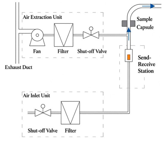
This study focuses on a vacuum-suction container-type pneumatic conveying system. Figure 1 shows a schematic diagram of the entire conveying system. The vacuum unit consists of a blower, a filter, and a shut-off valve, and the air inlet unit consists of a shut-off valve and a filter. The receiving and dispensing unit is used to receive and dispense sample vials and also includes a sample vial detector to monitor the number of sample vials being conveyed. The operating principle involves establishing a vacuum (negative pressure) through the vacuum unit and controlling the flow rate of the assist gas via the air inlet unit. Consequently, the conveyance of sample vials is primarily determined by the vacuum established by the vacuum unit and the gas flow rate provided by the air inlet unit.

Figure 1. Schematic diagram of vacuum-suction container-type pneumatic conveying system.

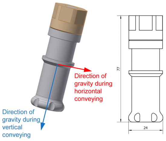
A three-dimensional geometric model of the sampling vial was created using SolidWorks (2018), as shown in Figure 2. The conveying pipeline has a nominal diameter (DN) of 32, corresponding to an inner diameter of 35.4 mm. The maximum external dimensions of the sampling vial are Φ24 × 77 mm. The sampling vial has a volume of 10 mL and can hold either an aqueous solution or an organic solution (empty vials were used in this study). To simplify the calculations, geometric models were created for both horizontal and vertical flow conditions (achieved by defining different directions of gravity for the sampling vial), and the simulation focused solely on the flow initiation process. The horizontal flow model consists of a horizontal straight pipe section, while the vertical flow model consists of a vertically rising pipe section, with a flow length of 200 mm.

Figure 2. Model of the sampling vial.

2.2. Finite Element Meshing

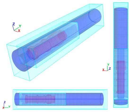
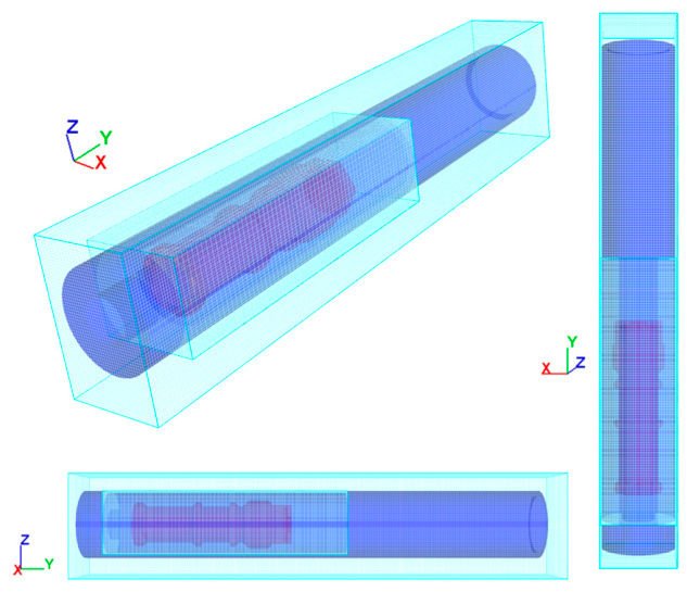
Meshing was performed using the preprocessing module of the CFD software. Cartesian structured finite-difference/control-volume mesh together with the fractional area-volume obstacle representation method was used to represent the vial and pipe-wall geometry (Figure 3). The meshing method describes solid boundaries on a Cartesian mesh using area fractions (AFs) and volume fractions (VFs), avoiding repeated reconstruction of body-fitted unstructured meshes at moving boundaries; it is particularly suitable for the FSI problem considered here [18]. To balance simulation accuracy and computational resources, the total number of mesh elements in the horizontal flow model was approximately 1,000,000, and the total number in the vertical flow model was approximately 60,000. The mesh was locally refined near the pipe wall and around the sampling vial to accurately capture the flow boundary layer and pressure gradients.

Figure 3. Meshing models of the sampling vial and pipe.

A systematic mesh-independence study and a formal y⁺ distribution analysis were not performed in the present work. The mesh sizes adopted here were selected to resolve the vial and the annular gap at the level recommended for CFD moving-object simulations while keeping the computational cost compatible with the parametric comparison objective of this study. A three-grid grid convergence index (GCI)-based refinement study, together with a time-step sensitivity analysis and experimental validation, is planned as the next stage of this research. The quantitative conclusions of this paper should therefore be interpreted as trend-level results within the stated operating ranges.

2.3. Physical Properties

The sampling vial is made of polyethylene with a density of 0.95 g/cm³. The gas phase is air, with a density of 1.225 kg/m³ and a dynamic viscosity μ = 1.781 × 10⁻⁵ Pa·s.

2.4. Model Assumptions

The air was treated as an incompressible Newtonian fluid with constant density and constant dynamic viscosity. The flow was solved in the incompressible flow mode with automatic limited-compressibility regularization, in which the density is constant and the pressure acts as a Lagrange multiplier enforcing zero divergence. The software can invoke limited-compressibility regularization to improve pressure convergence, in which a small density variation is permitted and kept below the approximately 1% criterion.

The flow was assumed to be isothermal, and the temperature-dependent Sutherland law for viscosity was not activated. The sampling vial was treated as a rigid body, and elastic deformation of the polyethylene wall was neglected. The pipe wall was treated as a no-slip boundary, and the vial surface was treated as a moving no-slip boundary through the GMO (general moving object) module. Vial–wall collisions were modeled with a partially elastic contact law. Only the 200 mm start-up section was simulated. Bends, long-distance friction losses, and the receiving-end deceleration process were not included. No mass transfer (evaporation, condensation, or leakage) was considered.

2.5. Boundary Conditions

The simulation employs a FSI method and accounts for the effects of gravity. For the horizontal flow model, the force of gravity is perpendicular to the pipe; for the vertical (upward) flow model, the force of gravity acts downward along the pipe’s axis. The gravitational acceleration was set to −9.81 m/s², and its direction is indicated in Figure 1. The boundary conditions were prescribed as a flow-inlet/pressure-outlet combination. At the upstream end of the pipe, a specified volumetric flow rate boundary was applied, with the gas volumetric flow rate Q prescribed as 0.001, 0.005, or 0.01 m³/s, and the ambient pressure at the inlet fixed at 101 kPa. At the downstream end, a specified pressure boundary was applied, with the vacuum level P prescribed as −3, −5, or −20 kPa. The surface of the sampling vial is treated as a fluid–structure interaction boundary. The CFD solver computes the aerodynamic force and torque by integrating the pressure and shear stress over the vial surface and solves the six-degree-of-freedom rigid-body motion of the vial. The specific values for vacuum pressure P and gas volumetric flow rate Q are shown in Table 1.

Table 1. Vacuum levels and gas flow rate settings for different pneumatic conveying sampling bottles.

Conveyance Method	No.	Vacuum Level P (kPa)	Gas Volume Flow Rate Q (m3/s)
Horizontal	1	−5	0.001
Horizontal	2	−5	0.005
Horizontal	3	−5	0.01
Vertical	4	−5	0.005
Vertical	5	−5	0.01
Vertical	6	−3	0.01
Vertical	7	−20	0.001

2.6. Control Equations

The governing equations are written in a non-conservative form on a fixed Cartesian grid using the fractional area/volume representation. The continuity equation, including the volume source induced by the moving vial, is

$${\displaystyle \frac{V_F}{\rho c^2}}{\displaystyle \frac{\partial p}{\partial t}}+{\displaystyle \frac{\partial \left(u{A}_x\right)}{\partial x}}+{\displaystyle \frac{\partial \left(v{A}_y\right)}{\partial y}}+{\displaystyle \frac{\partial \left(w{A}_z\right)}{\partial z}}=-{\displaystyle \frac{\partial V_F}{\partial t}}+{\displaystyle \frac{R_{\mathit{SOR}}}{\rho }}$$

(1)

$$-{\displaystyle \frac{\partial V_F}{\partial t}}={\displaystyle \frac{S_{\mathit{obj}}}{V_{\mathit{cell}}}}{V}_{\mathit{obj}}\cdot n$$

(2)

where V_F is the open volume fraction; u, v, and w are the velocity components in the x, y, and z directions; A_x, A_y, and A_z are the open area fractions; ρ is the air density; p is the pressure; c is the effective sound speed used in the limited-compressibility regularization; R_SOR is a mass source (zero here); and −∂V_F/∂t is the volume displacement produced by the rigid-body motion of the vial. S_obj is the surface area of the moving object in a mesh cell, the V_cell is the mesh-cell volume, V_obj is the velocity of the moving object, and n is outward unit normal vector. The momentum equations are

$${\displaystyle \frac{\partial u}{\partial t}}+{\displaystyle \frac{1}{V_F}}[u{A}_x{\displaystyle \frac{\partial u}{\partial x}}+v{A}_y{\displaystyle \frac{\partial u}{\partial y}}+w{A}_z{\displaystyle \frac{\partial u}{\partial z}}]=-{\displaystyle \frac{1}{\rho }}{\displaystyle \frac{\partial p}{\partial x}}+G_x+f_x-b_x-{\displaystyle \frac{R_{\mathit{SOR}}}{\rho V_F}}(u-u_w-\delta u_s)$$

(3)

$$\rho V_F{f}_x=\mathit{wsx}-\left[{\displaystyle \frac{\partial }{\partial x}}\right(A_x{\tau }_{\mathit{xx}})+{\displaystyle \frac{\partial }{\partial y}}(A_y{\tau }_{\mathit{xy}})+{\displaystyle \frac{\partial }{\partial z}}(A_z{\tau }_{\mathit{xz}}\left)\right]$$

(4)

$$\mathit{wsx}=-{\displaystyle \frac{2\mu }{A_x\delta x^2}}\left(1-A_x\right)\left(u-u_0\right)$$

(5)

where G_x is the body acceleration, f_x is the viscous acceleration including fractional area/volume representation area fractions, b_x is the porous-baffle loss (zero here), u_w is the velocity of the moving or source boundary, u_s is the relative velocity at the source surface, and wsx is the wall shear stress evaluated implicitly in Equation (5). Turbulence is closed with the RNG k–ε model:

$${\displaystyle \frac{\partial k}{\partial t}}+{\displaystyle \frac{1}{V_F}}[u{A}_x{\displaystyle \frac{\partial k}{\partial x}}+v{A}_y{\displaystyle \frac{\partial k}{\partial y}}+w{A}_z{\displaystyle \frac{\partial k}{\partial z}}]=P_T+G_T+{\mathrm{Diff}}_k-\epsilon$$

(6)

$${\displaystyle \frac{\partial \epsilon }{\partial t}}+{\displaystyle \frac{1}{V_F}}[u{A}_x{\displaystyle \frac{\partial \epsilon }{\partial x}}+v{A}_y{\displaystyle \frac{\partial \epsilon }{\partial y}}+w{A}_z{\displaystyle \frac{\partial \epsilon }{\partial z}}]=C_{\epsilon 1}{\displaystyle \frac{\epsilon }{k}}(P_T+C_{\epsilon 3}{G}_T)+{\mathrm{Diff}}_{\epsilon }-C_{\epsilon 2}{\displaystyle \frac{{\epsilon }^2}{k}}$$

(7)

$${\nu }_T=C_{\mu }{\displaystyle \frac{k^2}{\epsilon }}$$

(8)

$${\epsilon }_{\mathit{min}}=C_{\mu }^{3/4}{\displaystyle \frac{k^{3/2}}{L_T}}$$

(9)

with C_μ = 0.085, C_ε1 = 1.42, C_ε3 = 0.2, and the turbulent diffusion multiplier RMTKE = 1.39; C_ε2 is computed internally from the local turbulent kinetic energy k and shear production term P_T. Diff_k is the diffusion term in the k equation, and Diff_ε is the diffusion term in the ε equation. G_T is the Buoyancy production term, ν_T is the turbulent kinematic viscosity, ε_min is lower bound for the turbulent dissipation rate, and L_T is the maximum turbulent length scale.

The sampling vial was modeled as a 6-DOF rigid body using the GMO module with fully coupled FSI. The 6-DOF (degrees of freedom) motion of the vial is governed by Equations (10) and (11), with the aerodynamic force and torque obtained by integrating the pressure and shear stress over the fractional area/volume represented vial surface.

$$\mathbf{F}=m{\displaystyle \frac{d{\mathbf{V}}_G}{\mathit{dt}}}$$

(10)

$${\mathbf{T}}_G=\left[J\right]\cdot {\displaystyle \frac{\mathit{d\omega }}{\mathit{dt}}}+\omega \times \left(\right[J]\cdot \omega )$$

(11)

where F is the total force acting on the rigid body, m is the mass of the sampling vial, and V_G is the velocity of the rigid-body mass center; T_G is the total torque acting on the rigid body about its center of mass G, [J] is the moment of inertia tensor, and ω is the angular velocity vector. The vial–wall collision was treated with a partially elastic collision model with a restitution coefficient of 0.5 and a friction coefficient of 0.3; these values were selected to represent the polyethylene–steel contact pair.

Near-wall values of k and ε are imposed through the wall-function relations of Equations (12) and (13), where is u_∗ is the wall friction velocity, κ is the von Karman constant, and d is the normal distance from the wall.

The adaptive time step is limited by the convective Courant–Friedrichs–Lewy (CFL) condition (fluid should not traverse more than one cell per time step), Equation (14), and the viscous-diffusion limit, Equation (15), with a courant safety factor CON = 0.45. RM is the maximum viscosity multiplier for diffusion processes.

$$k={\displaystyle \frac{u_{*}^2}{\sqrt{C_{\mu }}}}$$

(12)

$$\epsilon ={\displaystyle \frac{u_{*}^3}{\mathit{\kappa d}}}$$

(13)

$$\delta t<\mathrm{CON}\cdot \mathit{min}({\displaystyle \frac{V_F\delta x}{A_x\left|u\right|}},{\displaystyle \frac{V_F\delta y}{A_y\left|v\right|}},{\displaystyle \frac{V_F\delta z}{A_z\left|w\right|}})$$

(14)

$$\delta t<{\displaystyle \frac{0.25}{\mathit{max}\left[\mathit{RM}\cdot \frac{\mu }{\rho }\left(\frac{1}{\delta x^2}+\frac{1}{\delta y^2}+\frac{1}{\delta z^2}\right)\right]}}$$

(15)

The time step is adjusted automatically according to the CFL stability condition and the viscous-diffusion limit, with a default maximum increment/decrement of 5% per cycle. When the stability condition is violated, the time step is halved and the solution is recalculated. The maximum time step was set to 1 × 10⁻⁴ s, and the initial time step was 1 × 10⁻⁶ s. Each simulation was run for a physical time of 1 s, sufficient for the vial to exit the 200 mm start-up section or to come to rest. Table 2 summarizes the numerical settings used in the CFD simulations.

Table 2. Summary of the numerical settings used in the CFD simulations.

Item	Setting
Solver	Finite-volume/finite-difference, transient, 3D
Mesh type	Cartesian structured grid with cut-cell boundary representation
Pressure–velocity coupling	Projection (time-splitting) method; Poisson equation for pressure correction
Poisson solver	GMRES; max iterations = 100 per time step; tolerance = 1 × 10−6
Convective discretization	First-order upwind
Temporal discretization	Explicit, adaptive time step
Time step	Initial 1 × 10−6 s; maximum 1 × 10−4 s; ±5% adjustment per cycle
Near-wall treatment	Standard wall function
Fluid–structure interaction	GMO, 6-DOF rigid body; force/moment by surface integration
Gravity	g = −9.81 m/s2 along the specified direction
Fluid	Air, incompressible; ρ = 1.225 kg/m3; μ = 1.781 × 10−5 Pa·s
Flow mode	Incompressible (automatic limited-compressibility regularization for pressure convergence)
Convergence criteria	Continuity residual < 1 × 10−3; GMRES residual < 1 × 10−6

3. Analysis of Results

3.1. Horizontal Conveying

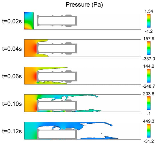
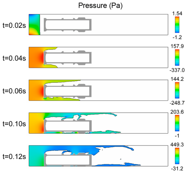
Under horizontal conveying conditions, various combinations of vacuum level P and gas volumetric flow rate Q were simulated. The simulation results showed that at a vacuum level of −5 kPa and a gas volumetric flow rate of 0.001 m³/s, the sampling vial tilted downward due to gravity and could not be propelled normally, resulting in a failure to convey gas (Figure 4). When the vacuum level remained at −5 kPa and the gas volumetric flow rate was increased to 0.005 m³/s, the sampling vial exhibited slight movement. Upon further increasing the gas volumetric flow rate to 0.01 m³/s, the sampling vial overcame the force of gravity and moved steadily forward along the pipeline.

Figure 4. The moving state of the horizontal conveying sampling vial over time and the pressure field of the airflow under the conditions of P = −5 kPa and Q = 0.001 m³/s.

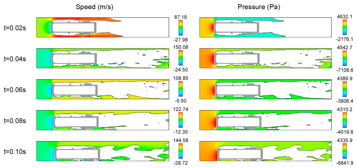
Figure 5 shows the movement of the sampling vial over time and the flow field during horizontal conveying under conditions of P = −5 kPa and Q = 0.005 m³/s. During the startup phase, at 0.02 s, gas flowed through the gap between the sampling vial and the pipe wall, generating a high-speed airflow of 87.18 m/s. At the rear end of the sampling vial, the airflow velocity was −27.98 m/s. At 0.04 s, the airflow distribution changed significantly: the upper airflow was relatively stable, while the lower airflow was turbulent. After 0.1 s, the sampling vial fell onto the pipe wall primarily due to gravity, having moved only a very short distance in the horizontal direction of flow; the airflow occupied the upper region between the sampling vial and the pipe wall. In the initial stage, the airflow passing through the gap between the sampling vial and the pipe wall generated a negative pressure of approximately −2.2 kPa, while the highest pressure in the flow was concentrated at the rear end of the sampling vial at approximately 4.6 kPa, which served to propel the sampling vial forward. However, the results showed that the maximum pressure of 4.6 kPa established at the rear end of the sampling vial was insufficient to propel the sampling vial forward.

Figure 5. The moving state of the horizontal conveying sampling vial over time and the velocity and pressure fields of the airflow under the conditions of P = −5 kPa and Q = 0.005 m³/s.

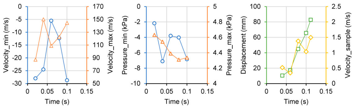
Figure 6 shows the time-dependent variations in maximum velocity, minimum velocity, maximum pressure, minimum pressure, sampling vial displacement, and sampling vial velocity for a horizontal gas flow field under operating conditions of P = −5 kPa and Q = 0.005 m³/s. Since the sampling vial did not move smoothly, the gas flow velocity exhibited significant fluctuations within 0.1 s, while the maximum pressure gradually decreased over time. Within 0.1 s, the sampling vial moved only about 80 mm before coming to rest against the pipe wall due to gravity, and its velocity did not accelerate further. Overall, the simulation data indicate that the sampling vial did not reach a stable conveying velocity under operating conditions of P = −5 kPa and Q = 0.005 m³/s.

Figure 6. The maximum velocity, minimum velocity, maximum pressure, minimum pressure, displacement of sampling vial, and variation of sampling vial velocity with time in the horizontal conveying gas flow field under the conditions of P = −5 kPa and Q = 0.005 m³/s.

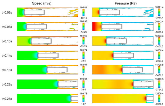
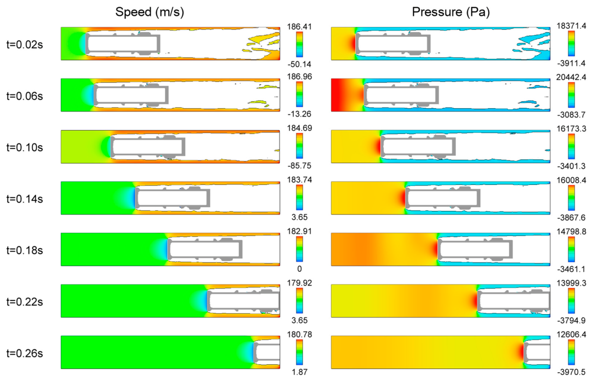
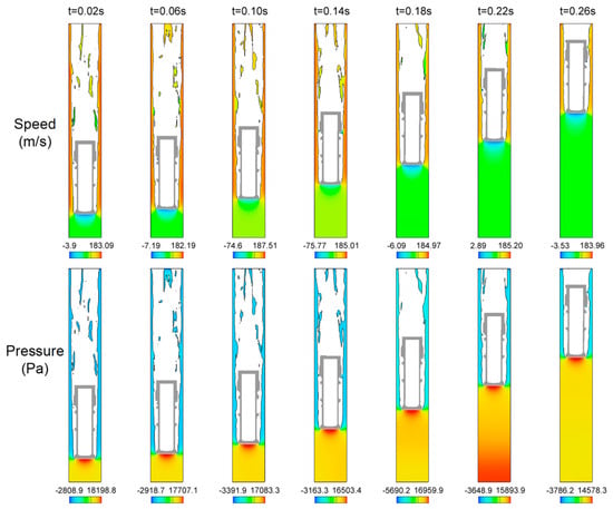
Figure 7 shows the movement of the horizontally transported sampling vial over time and the flow field under operating conditions of P = −5 kPa and Q = 0.01 m³/s. During the startup phase, the gas flow velocity fluctuates significantly but enters the gap between the sampling vial and the pipe wall symmetrically and gradually stabilizes. The maximum gas flow velocity is normally distributed within the gap between the sampling vial and the pipe wall, while the minimum velocity is distributed at the rear end plane of the sampling vial; during the startup phase, a reverse velocity is present, but after normal startup, the minimum velocity becomes positive. Furthermore, after normal startup and conveying, the gas flow velocity in the space at the rear end of the sampling vial is uniformly distributed. The airflow pressure field also exhibits some fluctuations during the startup phase; after normal startup, the variations become relatively stable. During horizontal conveying, the pressure distribution around the sampling vial exhibits distinct asymmetrical characteristics. The bottom of the sampling vial acts as the leeward side, where pressure is highest; pressure is lower on both sides of the vial body, while the vial head, as the windward side, maintains a set vacuum state. This pressure distribution pattern indicates that aerodynamic forces primarily act on the bottom of the sampling vial, propelling it forward; meanwhile, the negative pressure at the vial’s head creates a suction effect that helps maintain the sampling vial’s directional movement within the pipeline.

Figure 7. The moving state of the horizontal conveying sampling vial over time and the velocity and pressure fields of the airflow under the conditions of P = −5 kPa and Q = 0.01 m³/s.

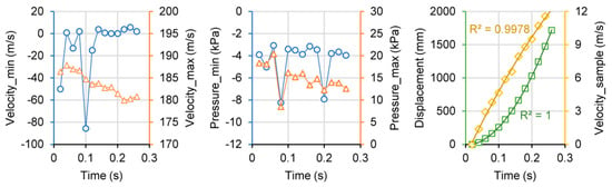
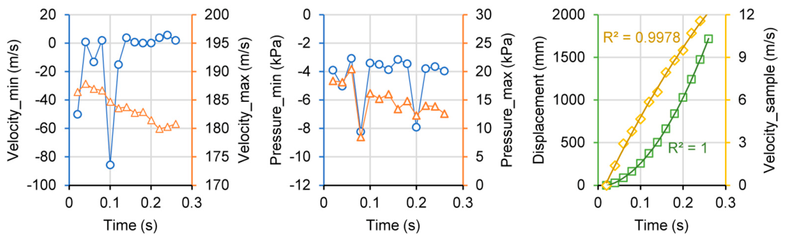
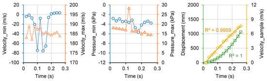
Figure 8 shows the time-dependent variations in maximum velocity, minimum velocity, maximum pressure, minimum pressure, sampling vial displacement, and sampling vial velocity for the horizontal gas flow field under operating conditions of P = −5 kPa and Q = 0.01 m³/s. During the startup phase from 0 to 0.1 s, the minimum velocity fluctuates significantly; after 0.12 s, the minimum velocity changes little; the maximum gas flow velocity gradually decreases to approximately 180 m/s. The maximum gas pressure—which also serves as the primary propulsive force at the rear end of the sampling vial—fluctuates significantly during the startup phase (0–0.1 s) but subsequently stabilizes, though it shows a decreasing trend; within 0.2 s, it drops from approximately 16 kPa to 12 kPa, indicating that the gas flow at the rear end becomes insufficient as the sampling vial continues to advance. The displacement of the sampling vial over time primarily follows a parabolic trend, with a quadratic polynomial fit having an R² of 1; the corresponding changes in the sampling vial’s velocity also exhibit an inverse parabolic trend, with the quadratic polynomial fit’s R² also approaching 1. Table 3 presents the corresponding quadratic polynomial equations for the sampling vial’s displacement and velocity, where t represents time (in seconds). Based on the fitting parameters of the quadratic polynomial equation for the sampling vial’s velocity, the maximum value of the parabolic curve can be calculated as 20.39 m/s, corresponding to a time of 0.68 s; that is, after 0.68 s, the sampling vial’s velocity can reach a conveying velocity of approximately 20 m/s, which exceeds the target of 10–15 m/s for actual industrial conveying velocity. Therefore, under operating conditions of P = −5 kPa and Q = 0.01 m³/s, a conveying velocity of 20 m/s for the sampling vial can be achieved.

Figure 8. The maximum velocity, minimum velocity, maximum pressure, minimum pressure, displacement of sampling vial, and variation of sampling vial velocity with time in the horizontal conveying gas flow field under the conditions of P = −5 kPa and Q = 0.01 m³/s.

Table 3. Fitting model and parameters for sampling vial displacement and velocity under different pneumatic conveying vacuum and gas flow conditions.

Conveyance Method	Vacuum Level P (kPa)	Gas Volume Flow Rate Q (m3/s)	Sampling Bottle Displacement (mm)	Sampling Bottle Velocity (m/s)
Horizontal	−5	0.01	−46.138t2 + 62.889t − 1.0442	24352t2 + 380.22t − 23.074
Vertical	−5	0.01	−19.563t2 + 36.513t − 0.5411	15193t2 + 177.12t − 10.577
Vertical	−3	0.01	−21.186t2 + 37.421t − 0.6680	14482t2 + 329.79t − 22.308

The resultant force on the vial in the GMO formulation consists of the aerodynamic force, gravity, and wall contact force. The aerodynamic force is obtained by integrating the pressure and shear stress over the vial surface. During start-up, the pressure at the tail end is high and the pressure at the front end is negative, producing a pressure-difference thrust F ≈ Δp · A_vial. In the horizontal case at P = −5 kPa and Q = 0.01 m³/s, the tail-end pressure during the start-up stage is approximately 16 kPa, and the corresponding thrust initially exceeds gravity plus friction, producing an average start-up velocity of approximately 6.5 m/s. As the vial velocity increases, the relative velocity between the gas and the vial decreases, the aerodynamic force decays (the tail-end pressure decreases from approximately 16 kPa to 12 kPa), and the acceleration therefore decreases—consistent with the concave velocity history observed.

3.2. Vertical Conveying

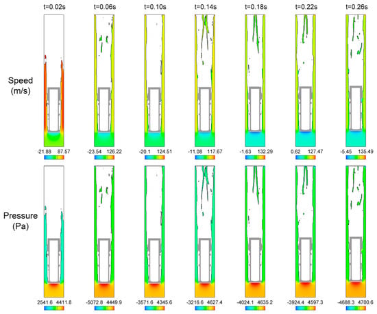
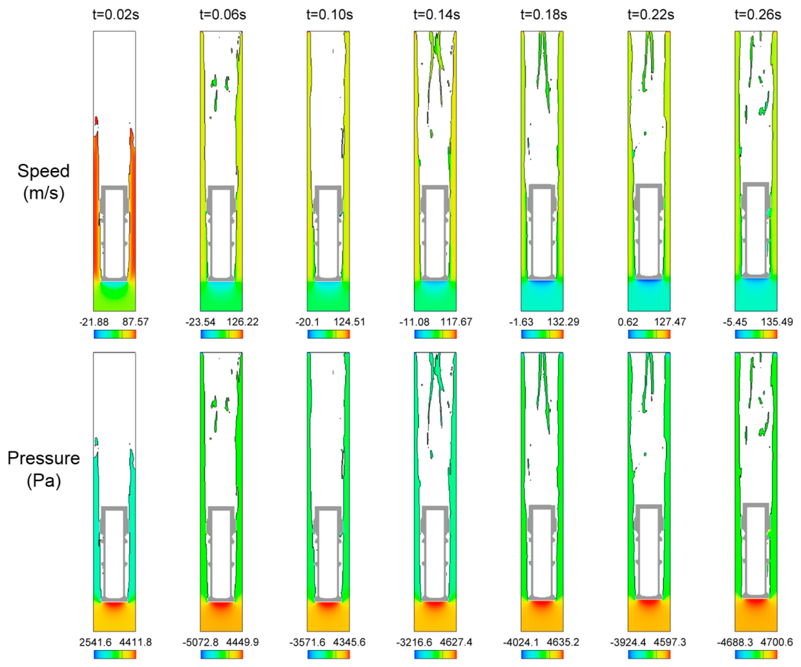
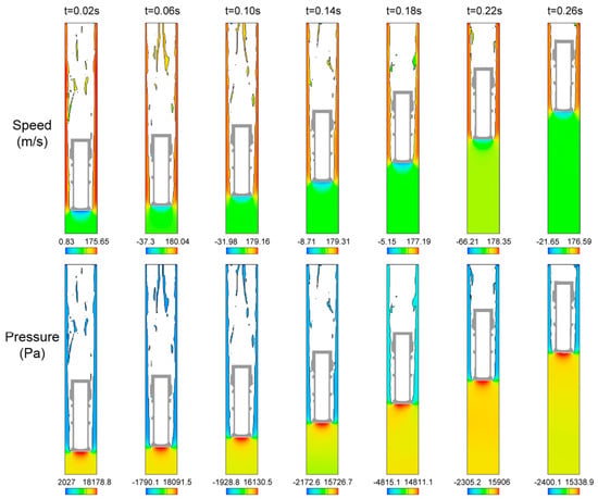
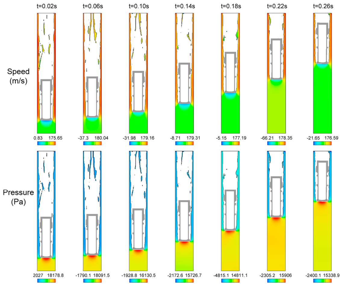
Figure 9 shows the movement of the sampling vial in the vertical (upward) direction over time and the flow field under operating conditions of P = −5 kPa and Q = 0.005 m³/s. During the startup phase, at 0.02 s, the flow field for vertical (upward) conveying exhibited characteristics similar to those of horizontal conveying: gas flowed through the gap between the sampling vial and the pipe wall, generating a high-speed gas flow of 87.57 m/s and a negative pressure of −2.5 kPa. The gas flow velocity at the rear end of the sampling vial was in the opposite direction, at −21.88 m/s; the gas thrust pressure during startup reached 4.4 kPa. At 0.06 s, the flow distribution also changed significantly, but the asymmetric flow caused by the gravitational effects of horizontal conveying did not occur; under vertical conveying conditions, the airflow continued to flow around the sampling vial. In the upper region of the sampling vial, after the airflow passed through, air was torn apart, with a maximum velocity reaching 126.22 m/s. The velocity and pressure distributions after 0.1 s were relatively similar; however, the maximum pressure of 4.7 kPa reached at the bottom of the sampling vial at 0.26 s was still insufficient to generate the force required to initiate the sampling vial, resulting in a failed push.

Figure 9. The moving state of the vertical upwards conveying sampling vial over time and the velocity and pressure fields of the airflow under the conditions of P = −5 kPa and Q = 0.005 m³/s.

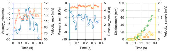
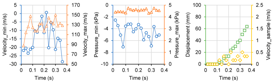
Figure 10 shows the time-dependent variations in maximum velocity, minimum velocity, maximum pressure, minimum pressure, sampling vial displacement, and sampling vial velocity for a vertical (upward) gas flow field under conditions of P = −5 kPa and Q = 0.005 m³/s. Within the first 0.4 s, the minimum gas flow velocities were all negative and exhibited significant fluctuations; the maximum velocity rose to over 110 m/s and continued to fluctuate thereafter. The corresponding minimum pressures were all negative. Although the maximum pressure remained relatively stable, the force generated was insufficient to propel the sampling vial, and thus propulsion did not occur. During the 0.1 s startup period, the sampling vial did not move significantly; thereafter, it underwent a slight displacement of approximately 60 mm. The corresponding velocity remained within 0.5 m/s and did not accelerate further.

Figure 10. The maximum velocity, minimum velocity, maximum pressure, minimum pressure, displacement of sampling vial, and variation of sampling vial velocity with time in the vertical upwards conveying gas flow field under the conditions of P = −5 kPa and Q = 0.005 m³/s.

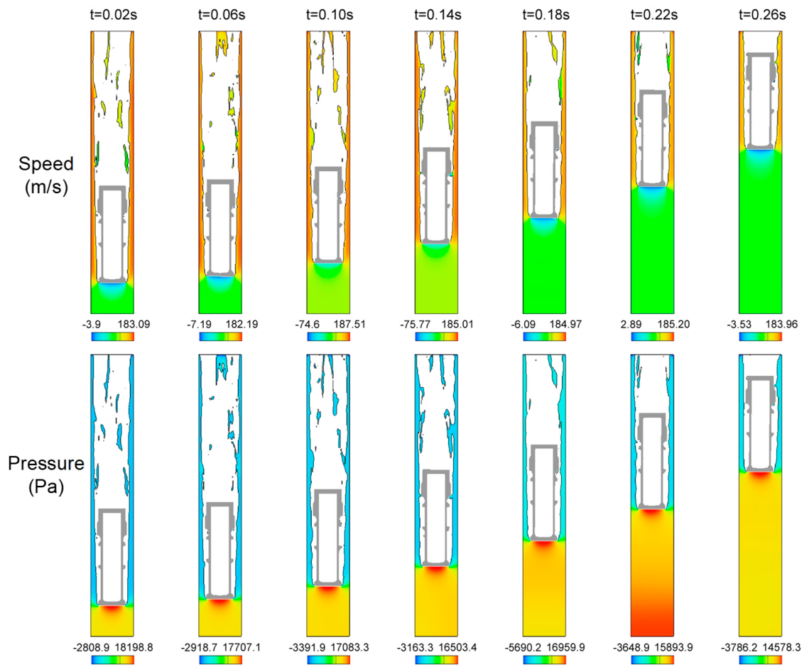
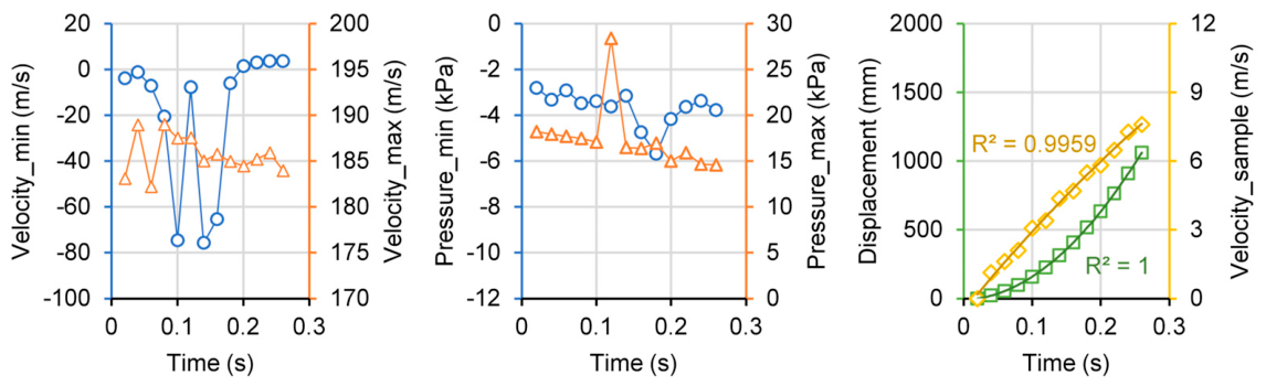
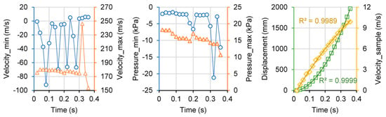
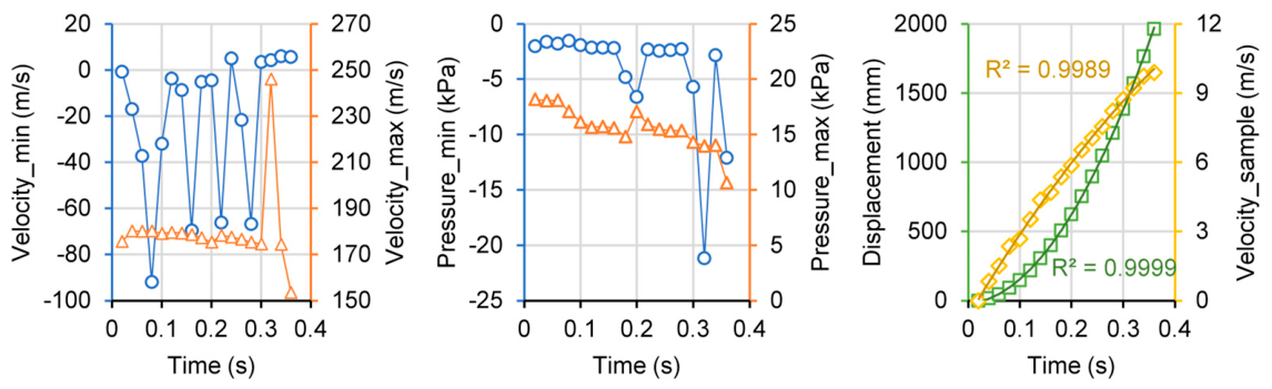
Figure 11 shows the movement of the sampling vial in the vertical (upward) direction over time and the flow field under operating conditions of P = −5 kPa and Q = 0.01 m³/s. Similar to horizontal conveying, the sampling vial was able to start and be transported normally when the gas flow rate was increased. During the startup phase, the flow field also exhibits significant fluctuations; after passing through the gap between the sampling vial and the pipe wall, the gas flow exhibits tearing turbulence; however, a relatively uniform velocity field is maintained at the rear end of the sampling vial. The pressure distribution is also similar to that observed in horizontal conveying: negative pressure exists around the sampling vial (i.e., at the front end of the conveying), while high pressure at the rear end of the sampling vial propels it upward. Figure 12 shows the time-dependent variations in maximum velocity, minimum velocity, maximum pressure, minimum pressure, sampling vial displacement, and sampling vial velocity for the vertical (upward) gas flow field under operating conditions of P = −5 kPa and Q = 0.01 m³/s. The gas flow velocity at the trailing end of the sampling vial is negative (i.e., in the opposite direction) during the 0–0.2 s interval; after 0.2 s, the minimum velocity becomes positive. The maximum gas flow velocity fluctuated somewhat during the startup phase from 0 to 0.1 s, after which it stabilized and gradually decreased. The gas pressure remained relatively stable overall, with the only fluctuation in maximum pressure occurring at 0.12 s; it generally trended downward from 18.2 kPa to 14.6 kPa. The displacement and velocity of the sampling vial followed parabolic trends. The parabolic curve for displacement, which gradually accelerates with time, has an upward-opening curve, with a coefficient of determination (R²) of 1; the velocity curve, on the other hand, follows an inverted parabolic curve with a downward-opening curve, with R² of 0.9959 (as shown in Table 3). Based on the fitting parameters of the quadratic polynomial for the sampling vial’s velocity, the maximum value of the parabolic curve was calculated to be 16.5 m/s, corresponding to a time of 0.93 s; indicating that after 0.93 s, the sampling vial’s velocity reached a conveying velocity of 16.5 m/s, exceeding the target industrial conveying velocity of 10–15 m/s. However, compared to horizontal conveying under the same operating conditions, this conveying velocity is lower by approximately 4 m/s, and the time to reach the maximum velocity is 0.25 s later. This is primarily due to the resistive effect of gravity in the vertical direction. Vertical upward conveying requires counteracting the downward force of gravity acting on the sampling vial; consequently, a higher thrust pressure at the bottom of the sampling vial is required to achieve the same velocity as in horizontal conveying. Therefore, under vertical conveying conditions, the sampling vial must perform work to overcome gravity, requiring greater aerodynamic force.

Figure 11. The moving state of the vertical upwards conveying sampling vial over time and the velocity and pressure fields of the airflow under the conditions of P = −5 kPa and Q = 0.01 m³/s.

Figure 12. The maximum velocity, minimum velocity, maximum pressure, minimum pressure, displacement of sampling vial, and variation of sampling vial velocity with time in the vertical upwards conveying gas flow field under the conditions of P = −5 kPa and Q = 0.01 m³/s.

When the vacuum level is reduced from −5 kPa to −3 kPa, with the gas volumetric flow rate Q = 0.01 m³/s remaining constant, the flow field conditions for the vertical (upward) conveying of the sampling vial remain largely unchanged. Figure 13 shows the movement of the sampling vial over time and the flow field during vertical (upward) conveying under operating conditions of P = −3 kPa and Q = 0.01 m³/s. Compared to the flow field under higher vacuum conditions, the distribution patterns of gas velocity and pressure are consistent, with only significant deviations in the velocity and pressure data. Figure 14 shows the time-dependent variations in maximum velocity, minimum velocity, maximum pressure, minimum pressure, sample vial displacement, and sample vial velocity for the vertical (upward) gas flow field under operating conditions of P = −3 kPa and Q = 0.01 m³/s. The minimum gas velocity at the rear end of the sample vial also exhibited significant fluctuations during the initial stage but turned positive after 0.3 s. The maximum velocity of the airflow around the sampling vial varied relatively steadily, with only a sudden spike in value at 0.32 s. The minimum pressure of the airflow remained relatively stable during the initial phase but fluctuated at 0.32 s; the maximum pressure at the trailing end of the sampling vial remained relatively stable, gradually decreasing from 18.2 kPa to 10 kPa. The displacement and velocity of the sampling vial also exhibited a distinct parabolic trend, with the R² values for the corresponding quadratic polynomial fits approaching 1 (as shown in Table 3). Based on the parameters of the quadratic polynomial fit for velocity, the maximum value of the parabolic curve was calculated to be 15.9 m/s, occurring at 0.88 s. The velocity of the sampling vial also exceeded the target industrial conveying velocity of 10–15 m/s. Compared to the −5 kPa vacuum condition, the velocity was only 0.64 m/s lower, but the time was reduced by 0.05 s. This indicates that for a gas volumetric flow rate of 0.01 m³/s, even a lower vacuum level is still sufficient to successfully propel the sampling vial.

Figure 13. The moving state of the vertical upwards conveying sampling vial over time and the velocity and pressure fields of the airflow under the conditions of P = −3 kPa and Q = 0.01 m³/s.

Figure 14. The maximum velocity, minimum velocity, maximum pressure, minimum pressure, displacement of sampling vial, and variation of sampling vial velocity with time in the vertical upwards conveying gas flow field under the conditions of P = −3 kPa and Q = 0.01 m³/s.

For vertical conveying, increasing Q from 0.005 to 0.01 m³/s (+100%) raises the maximum velocity from <0.5 m/s to 16.5 m/s, whereas reducing P from −5 to −3 kPa (−40%) changes the maximum velocity only from 16.5 to 15.9 m/s (−3.6%). This quantitatively shows flow-rate dominance.

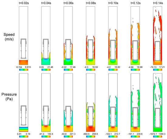
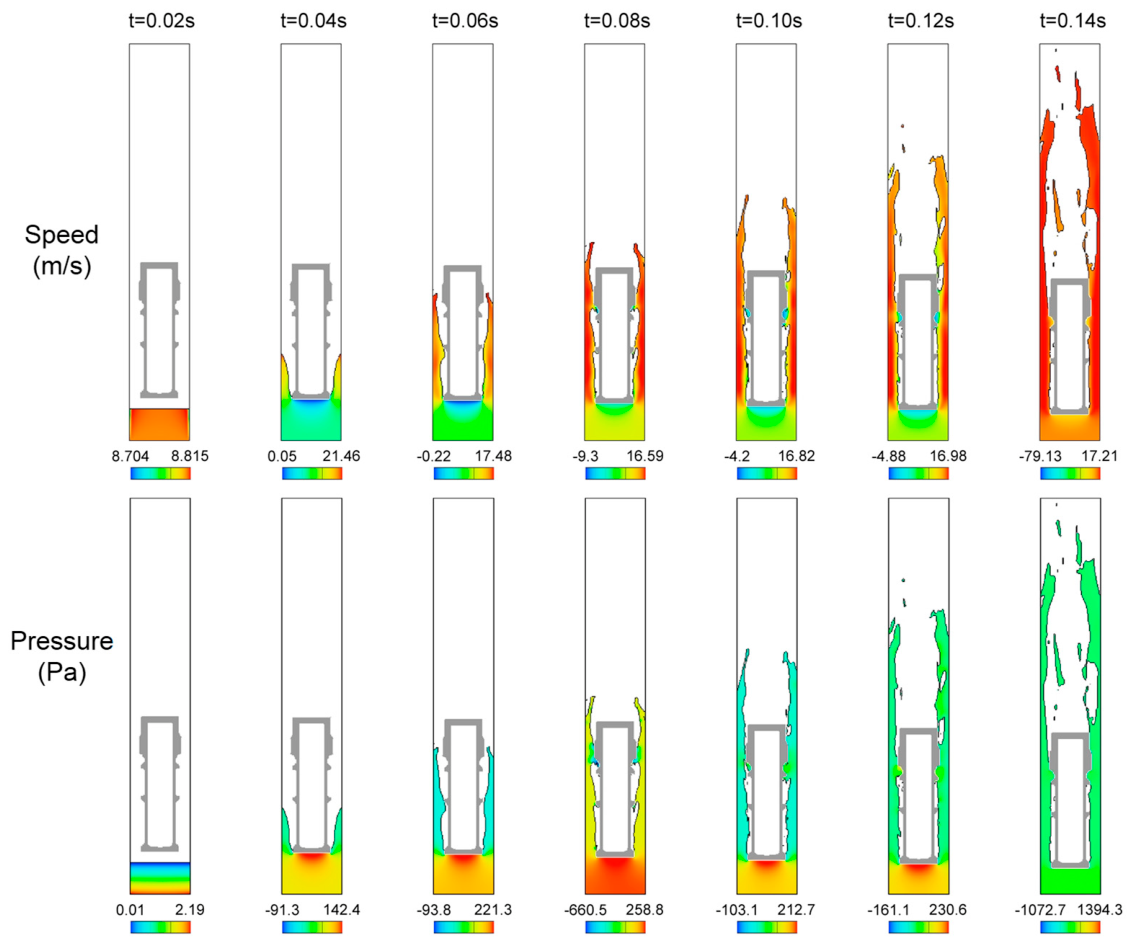
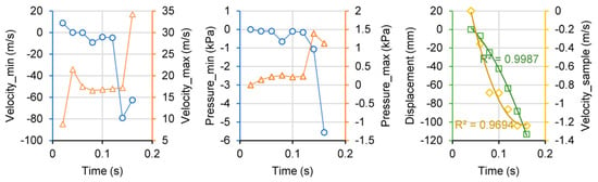
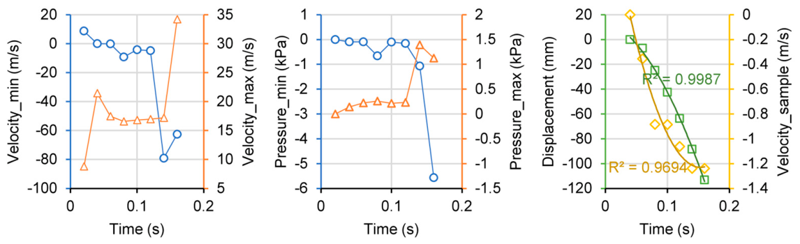
To verify whether gas conveying can be achieved under conditions of high vacuum and low gas volumetric flow rate, numerical simulations were performed under operating conditions of P = −20 kPa and Q = 0.001 m³/s. Figure 15 shows the movement of the sampling vial in the vertical (upward) direction over time and the flow field under the operating conditions of P = −20 kPa and Q = 0.001 m³/s. At 0.02 s, the gas had not yet reached the bottom of the sampling vial; at 0.04 s, it reached the bottom and began to enter the gap between the sampling vial and the pipe wall. At this point, the gas flow velocity around the sampling vial reached 21.46 m/s, but the pressure at the bottom of the sampling vial was only 0.14 kPa—completely insufficient to counteract the sampling vial’s weight. Consequently, the sampling vial gradually descended and moved downward. At 0.14 s, the maximum gas flow velocity reached only 17.21 m/s, and the maximum pressure of 1.39 kPa was also too low to propel the sampling vial. Figure 16 shows the variations over time of the maximum velocity, minimum velocity, maximum pressure, minimum pressure, displacement of the sampling vial, and velocity of the sampling vial in the vertical (upward) gas flow field under operating conditions of P = −20 kPa and Q = 0.001 m³/s. The results show that the maximum gas flow velocity is very low, and the maximum pressure is also insufficient. The displacement of the sampling vial follows a parabolic curve with the opening facing downward, gradually descending; the corresponding velocity also gradually decreases in the downward direction. Therefore, under conditions of high vacuum but insufficient gas volumetric flow rate, gas conveying via the sampling vial cannot be achieved.

Figure 15. The moving state of the vertical upwards conveying sampling vial over time and the velocity and pressure fields of the airflow under the conditions of P = −20 kPa and Q = 0.001 m³/s.

Figure 16. The maximum velocity, minimum velocity, maximum pressure, minimum pressure, displacement of sampling vial, and variation of sampling vial velocity with time in the vertical upwards conveying gas flow field under the conditions of P = −20 kPa and Q = 0.001 m³/s.

4. Conclusions

In this study, the start-up process of a radioactive liquid sampling vial in a vacuum-suction container-type pneumatic conveying system was simulated using a CFD–FSI approach. By synthesizing the simulation results for both horizontal and vertical conveying under various vacuum levels and gas volumetric flow rates, the following patterns of parameter influence can be summarized:

(1) Flow rate is the dominant operating parameter, while vacuum level plays a secondary role. For vertical upward conveying, increasing the gas volumetric flow rate from 0.005 to 0.01 m³/s (+100%) raised the maximum vial velocity from below 0.5 m/s to 16.5 m/s, whereas reducing the vacuum level from −5 to −3 kPa (−40%) changed the maximum velocity only from 16.5 to 15.9 m/s (−3.6%) and the time to reach it from 0.93 to 0.88 s.

(2) A minimum flow rate is required for successful start-up, and it cannot be replaced by a higher vacuum level. At Q = 0.001 m³/s, even when the vacuum level was increased to −20 kPa, the pressure at the bottom of the vial reached only 0.14 kPa, which was insufficient to overcome gravity, and the vial descended instead of being conveyed.

(3) The pressure field around the vial is strongly asymmetric. The tail end (leeward side) exhibits the highest pressure and the lowest airflow velocity, whereas the annular gap between the vial and the pipe wall exhibits the highest airflow velocity and a negative pressure. The thrust pressure at the tail end decays gradually as the vial accelerates, decreasing from approximately 16 kPa to 12 kPa in the horizontal case and from 18.2 kPa to 14.6 kPa in the vertical case (P = −5 kPa, Q = 0.01 m³/s).

(4) The vial velocity undergoes parabolic growth during start-up. Under P = −5 kPa and Q = 0.01 m³/s, the horizontal displacement and velocity were fitted by −46.138t² + 62.889t − 1.0442 and 24352t² + 380.22t − 23.074, respectively; the vertical counterparts were −19.563t² + 36.513t − 0.5411 and 15193t² + 177.12t − 10.577. The maximum velocity reached 20.39 m/s (horizontal) and 16.5 m/s (vertical) within the simulated period, both exceeding the target industrial range of 10–15 m/s.

(5) Vertical upward conveying requires a larger aerodynamic force than horizontal conveying. At the same operating conditions, the maximum velocity in vertical conveying was approximately 4 m/s lower than in horizontal conveying, and the time to reach the maximum was approximately 0.25 s longer, owing to the work required to overcome gravity.

(6) Low flow rates cause tilt instability. At Q = 0.005 m³/s, the vial in horizontal conveying tilted downward under gravity and failed to move normally, while in vertical conveying it exhibited only minimal movement (velocity < 0.5 m/s). Increasing the flow rate to 0.01 m³/s enabled the vial to overcome gravity, maintain a stable orientation, and move normally along the pipeline.

The equations describing the initiation of motion for the sampling vial and the critical operating parameters obtained in this study provide a mechanism analysis for the engineering design of pneumatic sampling systems for nuclear industry. Future work will build a transparent-pipe experimental rig equipped with high-speed imaging and pressure transducers to measure the vial velocity and the tail-end pressure, and will use these data to validate and, if necessary, recalibrate the numerical model.

5. Patents

This research has been granted four patents in China, namely: “Pass-through Detector and Pneumatic Conveyance System for Sample Conveyance” (Patent No. 202020016024.7), “A Sample Vial and Automatic Sampling Device” (Patent No. 202020009216.5), “A Receiving and Transmitting Device and a Pneumatic Sample Delivery System” (Patent No. 202122955174.1), and “Sample Vial” (Patent No. 202230674270.6).

References

- Kuang, S.; Zhou, M.; Yu, A. CFD-DEM modelling and simulation of pneumatic conveying: A review. Powder Technol. 2020, 365, 186–207. [Google Scholar] [CrossRef] [Scilit]
- Abe, M.C.; Gelladuga, G.A.; Mendoza, C.J.; Natavio, J.M.; Zabala, J.S.; Lopez, E.C.R. Pneumatic conveying technology: Recent advances and future outlook. Eng. Proc. 2023, 56, 205. [Google Scholar] [CrossRef] [Scilit]
- Bulatov, N.; Tastemir, N.; de Navascués, I.M.-P.; Rustembayev, A.; Karbayev, N. Mathematical modeling of vertical pneumatic conveying for solid waste transportation. Sci. Rep. 2026. [Google Scholar] [CrossRef] [Scilit] [PubMed]
- Klinzing, G.E. A review of pneumatic conveying status, advances and projections. Powder Technol. 2018, 333, 78–90. [Google Scholar] [CrossRef] [Scilit]
- Shao, Y.; Li, W.; Ma, C.; Feng, C. Application of pneumatic conveying technology in storage facility for radioactive waste liquid. At. Energy Sci. Technol. 2021, 55, 1914–1920. [Google Scholar]
- Wang, Z.; Yang, X.; Zhang, Z.; Gong, Y. Design and verification of vacuum pneumatic sample transport system in radio and chemical facilities. Guangdong Chem. Ind. 2022, 5, 92–93. [Google Scholar]
- Hu, R.; Wang, N.; Xu, B.; Zhang, H.; Li, L.; Cao, Y.; Zhu, S. Application of pneumatic conveying in reactor neutron spectroscopy sample transport. Nucl. Tech. 2023, 46, 020603. [Google Scholar]
- Bezrukov, A.S. Designing pneumatic conveying systems. Chem. Pet. Eng. 1967, 3, 129–132. [Google Scholar] [CrossRef] [Scilit]
- Ma, H.; Ma, G.; Sun, Z.; Gao, K. Flow characteristics of coarse particles in horizontal pneumatic conveying: A CFD-DEM study. Powder Technol. 2026, 482, 122715. [Google Scholar] [CrossRef] [Scilit]
- Wang, G.; Yang, S.; Zhang, X.; Wang, H. CFD-DEM investigation of slug dynamics in the vertical pneumatic conveying process. Chem. Eng. J. 2024, 496, 153473. [Google Scholar] [CrossRef] [Scilit]
- You, H.; Tan, G.; Ding, D.; Liu, Y.; Wang, L.; Ding, M.; Li, C.; Li, B.; Zhu, W. Transport behavior of shredded tobacco particles with different aspect ratios in pneumatic conveying using CFD-CGDEM. Powder Technol. 2027, 485, 123031. [Google Scholar] [CrossRef] [Scilit]
- Gu, X.; Yang, D.; Guo, A.; Zhang, M.; Zhang, S. ECVT imaging and CFD simulation of particle flow in a 90° bend. Powder Technol. 2025, 451, 120476. [Google Scholar] [CrossRef] [Scilit]
- Zhou, X.; Fang, F.; Li, Y. Numerical method for system level simulation of long-distance pneumatic conveying pipelines. Mathematics 2022, 10, 4073. [Google Scholar] [CrossRef] [Scilit]
- Fröhlig, S.; Bründl, P.; Straub, C.; Franke, J. Towards a simulation model for pneumatic conveying of cable-like deformable linear objects. In Proceedings of the 2025 IEEE International Conference on Industrial Engineering and Engineering Management (IEEM), Melbourne, Australia, 7–10 December 2025. [Google Scholar]
- Wang, Y.; Williams, K.; Jones, M.; Chen, B. CFD simulation methodology for gas-solid flow in bypass pneumatic conveying—A review. Appl. Therm. Eng. 2017, 125, 185–208. [Google Scholar] [CrossRef] [Scilit]
- Zhou, J.; Yan, X.; Zheng, Z.; Shangguan, L. Research status and prospect of key installations and flow characteristics of pneumatic conveying. Chin. J. Process Eng. 2023, 23, 649–661. [Google Scholar]
- Turkowski, M.; Szudarek, M. Pipeline system for transporting consumer goods, parcels and mail in capsules. Tunn. Undergr. Space Technol. 2019, 93, 103057. [Google Scholar] [CrossRef] [Scilit]
- Hirt, C.W. Volume-fraction techniques: Powerful tools for wind engineering. J. Wind Eng. Ind. Aerodyn. 1993, 46–47, 327–338. [Google Scholar] [CrossRef]
Disclaimer/Publisher’s Note: The statements, opinions and data contained in all publications are solely those of the individual author(s) and contributor(s) and not of MDPI and/or the editor(s). MDPI and/or the editor(s) disclaim responsibility for any injury to people or property resulting from any ideas, methods, instructions or products referred to in the content. |
© 2026 by the authors. Licensee MDPI, Basel, Switzerland. This article is an open access article distributed under the terms and conditions of the Creative Commons Attribution (CC BY) license.