Homogenization of Gas Flow in Deformable Porous Media with Wall-Slip

Abstract

Gas flow in deformable porous media couples wall slip, gas compressibility, and elastic pore-volume change. Two-scale asymptotic homogenization is used to derive periodic transport and elastic cell closures for a compressible Newtonian gas with first-order tangential slip and a linearly elastic solid. The macroscopic model combines effective stress balance, a Darcy law with geometry-dependent slip corrections, and conservative fluid mass storage. Its small-perturbation form separates gas compressibility from elastic storage. Two- and three-dimensional cells show that the importance of higher-order permeability corrections varies with pore configuration and $\mathrm{Kn}$. The effective elastic moduli and Biot coefficients also depend on porosity and loading direction. Exact channel solutions, limiting cases, and checks of the retained constitutive data support consistency of the formulation. The formulation describes quasi-static, small-strain transport in scale-separated periodic media within the continuum slip regime.

1. Introduction

Gas transport in small pores is affected by interactions between gas molecules and pore walls. Applications include microfluidic devices [1,2,3], deposition processes [4,5,6], and low-permeability reservoirs [7,8,9,10,11,12]. Wall slip in the continuum slip regime should be distinguished from Knudsen diffusion in the molecular regime [13]. Deformation can also change storage and transport in stress-sensitive rocks [14,15,16,17,18].

The conventional Knudsen number $\lambda /l$ compares the molecular mean free path $\lambda$ with a pore length $l$. Continuum, slip, transition, and free-molecular regimes are commonly associated with $\lambda /l$ below approximately ${10}^{-3}$, between ${10}^{-3}$ and 0.1, between 0.1 and 10, and above 10, respectively [19]. Here the wall coefficient $c$ is absorbed into $\mathrm{Kn}=c\lambda /l$. The first-order Maxwell or Navier condition describes tangential slip in the continuum slip regime [20]; higher-order boundary models introduce additional physical assumptions [21,22,23,24,25]. Small-strain elasticity and traction continuity describe the solid response [26,27,28,29,30,31].

Asymptotic homogenization and volume averaging both connect pore-scale boundary-value problems to effective coefficients [32,33,34]. Homogenization expands the fields in $\epsilon =l/L$ and derives periodic cell compatibility conditions, whereas volume averaging closes the fluctuations in averaged balances. Lasseux et al. [35] developed a rigid-medium slip-flow closure by volume averaging; Lasseux et al. [36] extended it to unsteady flow with dynamic permeability and memory. The present quasi-static formulation couples the transport closure to an elastic skeleton and compressible gas storage.

Higher-order rigid-medium permeability corrections provide an established basis for the transport expansion [35,37]. This study connects geometry-resolved slip permeability with elastic and storage coefficients in a common periodic framework. The derivation relates gas density changes and elastic pore-volume changes through a conservative mass balance, while the cell examples examine the influence of pore configuration. Related studies of deformable nanotubes [38] and confinement-dependent fluid properties [39] further motivate distinguishing wall deformation from constitutive changes under strong confinement.

Section 2 derives the periodic cell closures and macroscopic equations. Section 3 presents the two- and three-dimensional examples, analytical checks, and discussion of the results. Section 4 gives the conclusions.

2. Homogenization of Gas Slip Flow in Deformable Porous Media

2.1. Microscopic Model

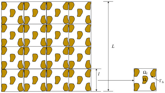
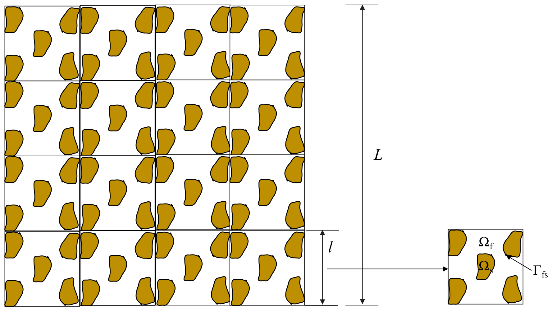
Consider a periodic cell $\mathsf{\Omega }={\mathsf{\Omega }}_{\mathrm{s}}\cup {\mathsf{\Omega }}_{\mathrm{f}}\cup {\mathsf{\Gamma }}_{\mathrm{fs}}$, with solid domain ${\mathsf{\Omega }}_{\mathrm{s}}$, fluid domain ${\mathsf{\Omega }}_{\mathrm{f}}$, and interface ${\mathsf{\Gamma }}_{\mathrm{fs}}$ (Figure 1). The reference solid is isotropic and linearly elastic, and the deformation is small. The molecular, pore, and macroscopic lengths satisfy $\lambda \ll l\ll L$.

$$\lambda \ll l\ll L$$

(1)

Figure 1. Schematic diagram of porous media.

The microscopic model consists of gas momentum and mass balances in ${\mathsf{\Omega }}_{\mathrm{f}}$, solid stress equilibrium in ${\mathsf{\Omega }}_{\mathrm{s}}$, an isothermal equation of state $f(p,{\rho }_{\mathrm{f}})=0$, traction continuity, and tangential slip on ${\mathsf{\Gamma }}_{\mathrm{fs}}$. The interface is impermeable in the solid frame: $(v-{\dot{u}}_{\mathrm{s}})\cdot n=0$. The normal $n$ points out of the fluid and into the solid.

$$\left\{\begin{array}{ll}di{v}_x{\sigma }_{\mathrm{s}}+{\rho }_{\mathrm{s}}g=0\hfill & \hfill \mathrm{in}\hspace{0.33em}{\mathsf{\Omega }}_{\mathrm{s}}\\ {\sigma }_{\mathrm{s}}=a:e\left(u_{\mathrm{s}}\right)\hfill & \hfill \mathrm{in}\hspace{0.33em}{\mathsf{\Omega }}_{\mathrm{s}}\\ di{v}_x{\sigma }_{\mathrm{f}}+{\rho }_{\mathrm{f}}g={\rho }_{\mathrm{f}}\left(\dot{v}+\left(v\cdot gra{d}_x\right)v\right)\hfill & \hfill \mathrm{in}\hspace{0.33em}{\mathsf{\Omega }}_{\mathrm{f}}\\ {\sigma }_{\mathrm{f}}=-pI+2\mu e\left(v\right)+\eta di{v}_{x}v\hfill & \hfill \mathrm{in}\hspace{0.33em}{\mathsf{\Omega }}_{\mathrm{f}}\\ {\dot{\rho }}_{\mathrm{f}}+di{v}_x\left({\rho }_{\mathrm{f}}v\right)=0\hfill & \hfill \mathrm{in}\hspace{0.33em}{\mathsf{\Omega }}_{\mathrm{f}}\\ f\left(p,{\rho }_{\mathrm{f}}\right)=0\hfill & \hfill \mathrm{in}\hspace{0.33em}{\mathsf{\Omega }}_{\mathrm{f}}\\ {\sigma }_{\mathrm{s}}\cdot n=\hspace{0.33em}{\sigma }_{\mathrm{f}}\cdot n\hfill & \hfill \mathrm{on}\hspace{0.33em}{\mathsf{\Gamma }}_{\mathrm{fs}}\\ v-{\dot{u}}_{\mathrm{s}}=-c\lambda n\cdot \left(gra{d}_{x}v+{\left(gra{d}_{x}v\right)}^T\right) \cdot \left(I-nn\right)\hfill & \hfill \hspace{1em}\hspace{1em}\mathrm{on}\hspace{0.33em}{\mathsf{\Gamma }}_{\mathrm{fs}}\end{array}\right.$$

(2)

Here ${\sigma }_{\mathrm{s}}$, $u_{\mathrm{s}}$, ${\rho }_{\mathrm{s}}$, and $a$ are the solid stress, displacement, density, and fourth-order stiffness tensor. The fluid variables ${\sigma }_{\mathrm{f}}$, $v$, ${\rho }_{\mathrm{f}}$, $p$, $\mu$, and $\eta$ denote stress, velocity, density, pressure, dynamic viscosity, and bulk viscosity; the bulk-viscous contribution to stress is $\eta (\mathrm{div}v)I$. A dot denotes time differentiation, $I$ is the identity tensor, and $c$ is the dimensionless slip coefficient. The mean free path $\lambda$ in the dilute hard-sphere estimate is defined by Equation (3).

$$\lambda ={\displaystyle \frac{k_{\mathrm{B}}T}{\sqrt{2}\pi d^{2}p}}$$

(3)

Here $k_{\mathrm{B}}=1.380649\times {10}^{-23} {\mathrm{JK}}^{-1}$ is Boltzmann’s constant, $T$ is absolute temperature, and $d$ is an effective molecular diameter. Equation (3) uses the dilute hard-sphere mean-free-path approximation.

The solid strain tensor $e(u_{\mathrm{s}})$ is defined by

$$e_{ij}={\displaystyle \frac{1}{2}}\left({\displaystyle \frac{\mathsf{\partial }{u}_{\mathrm{s}i}}{\mathsf{\partial }{x}_j}}+{\displaystyle \frac{\mathsf{\partial }{u}_{\mathrm{s}j}}{\mathsf{\partial }{x}_i}}\right)$$

(4)

The same symmetric-gradient definition applies to $e(v)$. The isotropic solid stiffness $a$ is expressed as

$$a_{ijkh}=\widehat{\lambda }{\delta }_{ij}{\delta }_{kl}+\widehat{\mu }\left({\delta }_{ik}{\delta }_{jl}+{\delta }_{il}{\delta }_{jk}\right)$$

(5)

The solid Lamé coefficients are ${\lambda }_s={\displaystyle \frac{E\nu }{(1+\nu )(1-2\nu )}}$ and ${\mu }_s={\displaystyle \frac{E}{2(1+\nu )}}$, denoted $\widehat{\lambda }$ and $\widehat{\mu }$ in the tensor formulas. $E$ and $\nu$ are the solid Young’s modulus and Poisson’s ratio. The stiffness has minor and major symmetries and is positive on nonzero symmetric strains for $E>0$ and $-1<\nu <1/2$.

$$a_{ijkh}=a_{jikh}=a_{ijhk}=a_{khij}$$

(6)

$$a_{ijkh}{z}_{ij}{z}_{kh}\ge a^{*}{z}_{ij}{z}_{ij}\begin{array}{cc},& a^{*}\end{array}>0$$

(7)

where $z_{ij}$ is a symmetric tensor.

Define the scale ratio $\epsilon =l/L\ll 1$, the Reynolds number $\mathrm{Re}$, transient Reynolds number $\mathrm{Rt}$, pressure-to-viscous ratio $Q$, and slip parameter $\mathrm{Kn}$ by Equations (8)–(12). In these equations $c$ is a slip coefficient, whereas $c_{ijkl}$ below denotes effective elastic stiffness.

$$\epsilon ={\displaystyle \frac{l}{L}}\ll 1$$

(8)

$$\mathrm{Re}={\displaystyle \frac{\left|{\rho }_{\mathrm{f}}\left(v\cdot \nabla \right)v\right|}{\left|\mu \Delta v\right|}}$$

(9)

$$\mathrm{Rt}={\displaystyle \frac{\left|{\rho }_{\mathrm{f}}\dot{v}\right|}{\left|\mu \Delta v\right|}}$$

(10)

$$Q={\displaystyle \frac{\left|\nabla p\right|}{\left|\mu \Delta v\right|}}$$

(11)

$$\mathrm{Kn}={\displaystyle \frac{c\lambda }{l}}$$

(12)

There is a related Strouhal number $S$

$$S={\displaystyle \frac{\left|{\dot{\rho }}_{\mathrm{f}}\right|}{\left|\nabla \cdot \left({\rho }_{\mathrm{f}}v\right)\right|}}={\displaystyle \frac{\left|{\rho }_{\mathrm{f}}\dot{v}\right|}{\left|{\rho }_{\mathrm{f}}\left(v\cdot \nabla \right)v\right|}}={\displaystyle \frac{\mathrm{Rt}}{\mathrm{Re}}}$$

(13)

Following the quasi-static scaling of Auriault et al. [40], take ${\mathrm{Re}}_L=O(1)$, ${\mathrm{Rt}}_L=O(1)$, $Q_L=O({\epsilon }^{-2})$, and $S_L=O(1)$. Resolving the pore derivatives places inertia above the leading viscous order in Equation (14), yielding the creeping-flow cell closure.

Under this scaling, Equation (2) becomes

$$\left\{\begin{array}{cc}di{v}_x{\sigma }_{\mathrm{s}}^{\epsilon }+{\rho }_{\mathrm{s}}g=0\hfill & \hfill \mathrm{in}\hspace{0.33em}{\mathsf{\Omega }}_{\mathrm{s}}\\ {\sigma }_{\mathrm{s}}^{\epsilon }=a:e_x\left(u_{\mathrm{s}}^{\epsilon }\right)\hfill & \hfill \mathrm{in}\hspace{0.33em}{\mathsf{\Omega }}_{\mathrm{s}}\\ di{v}_x{\sigma }_{\mathrm{f}}^{\epsilon }+{\rho }_{\mathrm{f}}^{\epsilon }g={\rho }_{\mathrm{f}}^{\epsilon }\left({\epsilon }^2{\dot{v}}^{\epsilon }+{\epsilon }^2\left(v^{\epsilon }\cdot gra{d}_x\right)v^{\epsilon }\right)\hfill & \hfill \mathrm{in}\hspace{0.33em}{\mathsf{\Omega }}_{\mathrm{f}}\\ {\sigma }_{\mathrm{f}}^{\epsilon }=-p^{\epsilon }I+2{\mu }^{\epsilon }{\epsilon }^{2}e\left(v^{\epsilon }\right)\hspace{0.33em}+\hspace{0.33em}{\eta }^{\epsilon }{\epsilon }^{2}di{v}_x{v}^{\epsilon }\hfill & \hfill \mathrm{in}\hspace{0.33em}{\mathsf{\Omega }}_{\mathrm{f}}\\ {\dot{\rho }}_{\mathrm{f}}^{\epsilon }+di{v}_x\left({\rho }_{\mathrm{f}}^{\epsilon }{v}^{\epsilon }\right)=0\hfill & \hfill \mathrm{in}\hspace{0.33em}{\mathsf{\Omega }}_{\mathrm{f}}\\ f\left(p^{\epsilon },{\rho }_{\mathrm{f}}^{\epsilon }\right)=0\hfill & \hfill \mathrm{in}\hspace{0.33em}{\mathsf{\Omega }}_{\mathrm{f}}\\ {\sigma }_{\mathrm{s}}^{\epsilon }\cdot n=\hspace{0.33em}{\sigma }_{\mathrm{f}}^{\epsilon }\cdot n\hfill & \hfill \mathrm{on}\hspace{0.33em}{\mathsf{\Gamma }}_{\mathrm{fs}}\\ v^{\epsilon }-{\dot{u}}_s^{\epsilon }=-\mathrm{Kn}\epsilon n\cdot \left(gra{d}_x{v}^{\epsilon }+{\left(gra{d}_x{v}^{\epsilon }\right)}^T\right)\cdot \left(I-nn\right)\hfill & \hfill \hspace{1em}\mathrm{on}\hspace{0.33em}{\mathsf{\Gamma }}_{\mathrm{fs}}\end{array}\right.$$

(14)

Equation (14) uses $L$-normalized spatial derivatives. Its boundary slip length is $c\lambda /L=\epsilon \mathrm{Kn}$; the pore derivative ${\epsilon }^{-1}{\nabla }_y$ therefore gives an $O(\mathrm{Kn})$ slip condition at cell scale.

2.2. Asymptotic Expansion

Introduce slow and fast coordinates $x$ and $y=x/\epsilon$. Homogenization is performed at fixed small $\mathrm{Kn}=c\lambda /l$, followed by expansion of the leading transport cell solution about $\mathrm{Kn}=0$. Thus $\epsilon \mathrm{Kn}=c\lambda /L$, with no imposed relation $\mathrm{Kn}=\epsilon$.

$$y={\epsilon }^{-1}x$$

(15)

Consequently, the derivative operator becomes

$$\nabla ={\nabla }_x+{\epsilon }^{-1}{\nabla }_y$$

(16)

Here ${\nabla }_x$ and ${\nabla }_y$ act on the slow and fast coordinates, and each expansion coefficient is periodic in $y$. A separate perturbation amplitude $\delta$ measures displacement gradients, relative pressure increments, and relative velocity about a no-flow equilibrium. The reference-cell elastic and storage closure retains $O(\delta )$ terms; $\delta$ is independent of $\epsilon$ and $\mathrm{Kn}$.

$$\begin{array}{l}{u}_{\mathrm{s}}^{\epsilon }=u_{\mathrm{s}}^{\left(0\right)}\left(x,y,t\right)+\epsilon u_{\mathrm{s}}^{\left(1\right)}\left(x,y,t\right)+{\epsilon }^2{u}_{\mathrm{s}}^{\left(2\right)}\left(x,y,t\right)+\cdots \\ v^{\epsilon }=v^{\left(0\right)}\left(x,y,t\right)+\epsilon v^{\left(1\right)}\left(x,y,t\right)+{\epsilon }^2{v}^{\left(2\right)}\left(x,y,t\right)+\cdots \\ p^{\epsilon }=p^{\left(0\right)}\left(x,y,t\right)+\epsilon p^{\left(1\right)}\left(x,y,t\right)+{\epsilon }^2{p}^{\left(2\right)}\left(x,y,t\right)+\cdots \\ {\rho }_{\mathrm{f}}^{\epsilon }={\rho }_{\mathrm{f}}^{\left(0\right)}\left(x,y,t\right)+\epsilon {\rho }_{\mathrm{f}}^{\left(1\right)}\left(x,y,t\right)+{\epsilon }^2{\rho }_{\mathrm{f}}^{\left(2\right)}\left(x,y,t\right)+\cdots \\ {\sigma }_{\mathrm{s}}^{\epsilon }={\epsilon }^{-1}{\sigma }_{\mathrm{s}}^{\left(-1\right)}\left(x,y,t\right)+{\sigma }_{\mathrm{s}}^{\left(0\right)}\left(x,y,t\right)+\epsilon {\sigma }_{\mathrm{s}}^{\left(1\right)}\left(x,y,t\right)+\cdots \end{array}$$

(17)

where

$$\begin{array}{l}{\sigma }_{\mathrm{s}}^{\left(-1\right)}=a:e_y\left(u_{\mathrm{s}}^{\left(0\right)}\right)\\ {\sigma }_{\mathrm{s}}^{\left(0\right)}=a:\left[e_x\left(u_{\mathrm{s}}^{\left(0\right)}\right)+e_y\left(u_{\mathrm{s}}^{\left(1\right)}\right)\right]\\ {\sigma }_{\mathrm{s}}^{\left(1\right)}=a:\left[e_x\left(u_{\mathrm{s}}^{\left(1\right)}\right)+e_y\left(u_{\mathrm{s}}^{\left(2\right)}\right)\right]\hspace{0.33em}\end{array}$$

(18)

The equation of state and the pressure-dependent $\mu$, $\eta$, and $\mathrm{Kn}$ are expanded about $p^{(0)}$. The relation between ${\rho }_{\mathrm{f}}^{(1)}$ and $p^{(1)}$ is given in Section 2.6. All cell coefficients are evaluated on the reference geometry.

2.3. Cell Correctors

Substitution of the expansions into Equation (14) gives the leading solid equilibrium and interface conditions:

$$\begin{array}{l}di{v}_y{\sigma }_{\mathrm{s}}^{\left(-1\right)}=di{v}_y\left(a:e_y\left(u_{\mathrm{s}}^{\left(0\right)}\right)\right)= 0\mathrm{in}\hspace{0.33em}{\mathsf{\Omega }}_{\mathrm{s}}\\ {\sigma }_{\mathrm{s}}^{\left(-1\right)}\cdot n=\hspace{0.33em}a:e_y\left(u_{\mathrm{s}}^{\left(0\right)}\right)\cdot n=0\mathrm{on}\hspace{0.33em}{\mathsf{\Gamma }}_{\mathrm{fs}}\end{array}$$

(19)

Coercivity of the elastic energy, periodicity, and connectedness of the solid frame imply that the leading solid displacement is independent of $y$ after the rigid-translation mode is fixed:

$$u_{\mathrm{s}}^{\left(0\right)}=u_{\mathrm{s}}^{\left(0\right)}\left(x,t\right)$$

(20)

The leading gas momentum balance and equation of state give

$$\begin{array}{l}gra{d}_y{p}^{\left(0\right)}=0\mathrm{in}\hspace{0.33em}{\mathsf{\Omega }}_{\mathrm{f}}\\ f\left(p^{\left(0\right)},{\rho }_{\mathrm{f}}^{\left(0\right)}\right)=0\mathrm{in}\hspace{0.33em}{\mathsf{\Omega }}_{\mathrm{f}}\hspace{0.33em}\end{array}$$

(21)

Consequently, the leading pressure and density are independent of $y$:

$$p^{\left(0\right)}=p^{\left(0\right)}\left(x,t\right), {\rho }_{\mathrm{f}}^{\left(0\right)}={\rho }_{\mathrm{f}}^{\left(0\right)}\left(x,t\right)$$

(22)

At the next elastic order, the solid equilibrium and traction conditions become

$$\begin{array}{l}di{v}_y{\sigma }_{\mathrm{s}}^{\left(0\right)}=di{v}_y\left(a:\left[e_x\left(u_{\mathrm{s}}^{\left(0\right)}\right)+e_y\left(u_{\mathrm{s}}^{\left(1\right)}\right)\right]\right)= 0\mathrm{in}\hspace{0.33em}{\mathsf{\Omega }}_{\mathrm{s}}\\ {\sigma }_{\mathrm{s}}^{\left(0\right)}\cdot n=\hspace{0.33em}a:\left[e_x\left(u_{\mathrm{s}}^{\left(0\right)}\right)+e_y\left(u_{\mathrm{s}}^{\left(1\right)}\right)\right]\cdot n=-p^{\left(0\right)}n\mathrm{on}\hspace{0.33em}{\mathsf{\Gamma }}_{\mathrm{fs}}\end{array}$$

(23)

The first solid-displacement corrector has the form

$$u_{\mathrm{s}}^{\left(1\right)}=\xi \left(y\right):e_x\left(u_{\mathrm{s}}^{\left(0\right)}\right)-\zeta \left(y\right)p^{\left(0\right)}+{\overline{u}}_{\mathrm{s}}^{\left(1\right)}\left(x,t\right)$$

(24)

The third-order tensor $\xi$ consists of displacement correctors for imposed symmetric unit strains and solves the following problem:

$$\begin{array}{cc}{\mathrm{div}}_y[a:e_y({\xi }^{kh})]& =0\hspace{1em}\mathrm{in}\hspace{0.33em}{\mathsf{\Omega }}_{\mathrm{s}}\\ a:e_y({\xi }^{kh})\cdot n& =-a:E^{kh}\cdot n\hspace{1em}\mathrm{on}\hspace{0.33em}{\mathsf{\Gamma }}_{\mathrm{fs}}\end{array}$$

(25)

For the loading pair $(k,h)$, use the symmetric unit-strain tensor $E^{kh}$ with components

$$E_{ij}^{kh}={\displaystyle \frac{1}{2}}({\delta }_{ik}{\delta }_{jh}+{\delta }_{ih}{\delta }_{jk})$$

(26)

The pressure-loading corrector $\zeta$ satisfies the following problem, with its sign consistent with the displacement contribution $-\zeta p$ in Equation (24):

$$\begin{array}{cc}{\mathrm{div}}_y[a:e_y(\zeta )]& =0\hspace{1em}\mathrm{in}\hspace{0.33em}{\mathsf{\Omega }}_{\mathrm{s}}\\ a:e_y(\zeta )\cdot n& =I\cdot n\hspace{1em}\mathrm{on}\hspace{0.33em}{\mathsf{\Gamma }}_{\mathrm{fs}}\end{array}$$

(27)

Periodic displacement fluctuations and anti-periodic outer-face tractions cancel on paired faces; a zero cell mean fixes the rigid translation in the theoretical correctors. The finite-element implementation instead fixes one reference point, which gives the same strains and averaged stresses. The constant-pressure and symmetric unit-strain interface loads have zero resultant over the periodically extended cell. A connected load-bearing solid and coercive constituent stiffness give uniqueness modulo translation.

For a solenoidal Stokes corrector with normal boundary velocity $g_n$, periodicity requires $\underset{{\mathsf{\Gamma }}_{\mathrm{fs}}}{{\displaystyle \int }}{g}_{n}dS=0$ on each connected fluid component. The relative-velocity hierarchy satisfies this at every slip order because its boundary data are tangential. A pressure gauge on each connected fluid component completes the specification, including separate through-going capillaries. The next-order compressible mass equation supplies the nonhomogeneous compatibility relation (56).

The effect of interface motion on macroscopic storage is derived through the material pore volume in Section 2.6.

2.4. Effective Stress

The next-order stress balances and interface traction continuity give

$$\begin{array}{cc}di{v}_x{\sigma }_{\mathrm{s}}^{\left(0\right)}+di{v}_y{\sigma }_{\mathrm{s}}^{\left(1\right)}+{\rho }_{\mathrm{s}}g=0\hfill & \hfill \mathrm{in}\hspace{0.33em}{\mathsf{\Omega }}_{\mathrm{s}}\\ di{v}_y{\sigma }_{\mathrm{f}}^{\left(1\right)}-gra{d}_x{p}^{\left(0\right)}+{\rho }_{\mathrm{f}}^{\left(0\right)}g=0\hfill & \hfill \hspace{0.33em}\mathrm{in}\hspace{0.33em}{\mathsf{\Omega }}_{\mathrm{f}}\\ {\sigma }_{\mathrm{s}}^{\left(1\right)}\cdot n=\hspace{0.33em}{\sigma }_{\mathrm{f}}^{\left(1\right)}\cdot n\hfill & \hfill \mathrm{on}\hspace{0.33em}{\mathsf{\Gamma }}_{\mathrm{fs}}\end{array}$$

(28)

Then the total stress is defined as

$${\sigma }^{\mathrm{T}}=\left\{\begin{array}{l}{\sigma }_{\mathrm{s}}\mathrm{in} {\mathsf{\Omega }}_{\mathrm{s}}\\ {\sigma }_{\mathrm{f}}\mathrm{in} {\mathsf{\Omega }}_{\mathrm{f}}\end{array}\right.$$

(29)

Use the superficial phase average ${⟨a⟩}_{\beta }=|\mathsf{\Omega }{|}^{-1}\underset{{\mathsf{\Omega }}_{\beta }}{{\displaystyle \int }}adV$, $\beta =s,f$, normalized by the whole cell volume. Hence $\phi =\left|{\mathsf{\Omega }}_{\mathrm{f}}\right|/\left|\mathsf{\Omega }\right|$ and ${⟨1⟩}_{\mathrm{f}}=\phi$.

$$⟨\cdot ⟩={\displaystyle \frac{1}{\left|\mathsf{\Omega }\right|}}{\displaystyle {\int }_{{\mathsf{\Omega }}_{\beta }}\cdot }d{\mathsf{\Omega }}_{\beta }\begin{array}{cc},& \beta =\mathrm{s},\mathrm{f}\end{array}$$

(30)

Averaging Equation (28) and applying the divergence theorem gives

$$di{v}_x⟨{\sigma }_{\mathrm{s}}^{\left(0\right)}⟩+{\displaystyle \frac{1}{\left|\mathsf{\Omega }\right|}}{\displaystyle {\int }_{{\mathsf{\Gamma }}_{\mathrm{fs}}}{\sigma }_{\mathrm{s}}^{\left(1\right)}\cdot ndS+⟨{\rho }_{\mathrm{s}}⟩g=0}$$

(31)

$${\displaystyle \frac{1}{\left|\mathsf{\Omega }\right|}}{\displaystyle {\int }_{{\mathsf{\Gamma }}_{\mathrm{fs}}}{\sigma }_{\mathrm{f}}^{\left(1\right)}\cdot ndS}+\varphi gra{d}_x{p}^{\left(0\right)}-⟨{\rho }_{\mathrm{f}}^{\left(0\right)}⟩g=0$$

(32)

Combining Equations (31) and (32) with interface traction continuity yields

$$di{v}_x⟨{\sigma }^{\mathrm{T}\left(0\right)}⟩+⟨\rho ⟩g=di{v}_x⟨{\sigma }_{\mathrm{s}}^{\left(0\right)}⟩-\varphi gra{d}_x{p}^{\left(0\right)}+⟨\rho ⟩g=0$$

(33)

where the density of the bulk material is defined by

$$\rho =\left\{\begin{array}{l}{\rho }_{\mathrm{s}}\mathrm{in} {\mathsf{\Omega }}_{\mathrm{s}}\\ {\rho }_{\mathrm{f}}\mathrm{in} {\mathsf{\Omega }}_{\mathrm{f}}\end{array}\right.$$

(34)

Substitution of the constitutive relation and Equation (24) gives the effective stress law (35), with the second-order Biot tensor $\alpha$.

$$\begin{array}{c}di{v}_x⟨{\sigma }^{\mathrm{T}\left(0\right)}⟩+⟨\rho ⟩g=0\\ ⟨{\sigma }^{\mathrm{T}\left(0\right)}⟩=c:e_x\left(u_{\mathrm{s}}^{\left(0\right)}\right)\hspace{0.33em}-\alpha p^{\left(0\right)}\end{array}$$

(35)

where the effective elastic tensor and Biot coefficient are defined by

$$c_{ijkh}=⟨a_{ijkh}+a_{ijlm}{e}_{ylm}\left({\xi }^{kh}\right)⟩$$

(36)

$${\alpha }_{ij}=\varphi I_{ij}+⟨a_{ijlm}{e}_{ylm}\left(\zeta \right)⟩$$

(37)

2.5. Slip Corrected Darcy Law

The leading gas momentum balance, mass balance, and slip condition read

$$\begin{array}{cc}{\mu }^{\left(0\right)}{\Delta }_y{v}^{\left(0\right)}-gra{d}_x{p}^{\left(0\right)}-gra{d}_y{p}^{\left(1\right)}+{\rho }_{\mathrm{f}}^{\left(0\right)}g=0\hfill & \hfill \mathrm{in}\hspace{0.33em}{\mathsf{\Omega }}_{\mathrm{f}}\\ di{v}_y{v}^{\left(0\right)}=0\hfill & \hfill \mathrm{in}\hspace{0.33em}{\mathsf{\Omega }}_{\mathrm{f}}\\ v^{\left(0\right)}-{\dot{u}}_{\mathrm{s}}^{\left(0\right)}=-{\mathrm{Kn}}^{\left(0\right)}n\cdot \left(gra{d}_y{v}^{\left(0\right)}+{\left(gra{d}_y{v}^{\left(0\right)}\right)}^T\right)\cdot \left(I-nn\right)\hfill & \hfill \hspace{1em}\mathrm{on}\hspace{0.33em}{\mathsf{\Gamma }}_{\mathrm{fs}}\end{array}$$

(38)

Define the pore-scale relative velocity $\omega =v^{(0)}-{\dot{u}}_{\mathrm{s}}^{(0)}$. Its superficial average $q={⟨\omega ⟩}_{\mathrm{f}}={⟨v^{(0)}⟩}_{\mathrm{f}}-\phi {\dot{u}}_{\mathrm{s}}^{(0)}$ is the Darcy flux relative to the solid.

$$\begin{array}{cc}{\mu }^{\left(0\right)}{\Delta }_y\omega -gra{d}_x{p}^{\left(0\right)}-gra{d}_y{p}^{\left(1\right)}+{\rho }_{\mathrm{f}}^{\left(0\right)}g=0\hfill & \hfill \mathrm{in}\hspace{0.33em}{\mathsf{\Omega }}_{\mathrm{f}}\\ di{v}_y\omega =0\hfill & \hfill \mathrm{in}\hspace{0.33em}{\mathsf{\Omega }}_{\mathrm{f}}\\ \omega =-{\mathrm{Kn}}^{\left(0\right)}n\cdot \left(gra{d}_y\omega +{\left(gra{d}_y\omega \right)}^T\right)\cdot \left(I-nn\right)\hfill & \hfill \hspace{1em}\hspace{1em}\mathrm{on}\hspace{0.33em}{\mathsf{\Gamma }}_{\mathrm{fs}}\end{array}$$

(39)

The relative velocity and pressure corrector are linear in the macroscopic forcing, and can be written as

$$\begin{array}{l}\omega =\theta \cdot \left({\rho }_{\mathrm{f}}^{\left(0\right)}g-gra{d}_x{p}^{\left(0\right)}\right)\\ p^{\left(1\right)}=\tau \cdot \left(gra{d}_x{p}^{\left(0\right)}-{\rho }_{\mathrm{f}}^{\left(0\right)}g\right)+{\overline{p}}^{\left(1\right)}\end{array}$$

(40)

Here $\theta$ is the velocity response and $\tau$ is the vector of periodic pressure responses in Equation (40). Each pressure response has zero intrinsic mean on its connected fluid component. Define $G={\nabla }_x{p}^{(0)}-{\rho }_{\mathrm{f}}^{(0)}g$, so $p^{(1)}={\tau }_j{G}_j+{\overline{p}}^{(1)}$. The zero-mean convention fixes the additive constant in each cell-pressure fluctuation.

Expand the transport responses in ${\mathrm{Kn}}^{(0)}$ near zero. This is an expansion of the specified first-order-slip continuum cell solution, so the power of $\mathrm{Kn}$ denotes truncation order rather than kinetic boundary-model order.

$$\omega ={\omega }^0+{\mathrm{Kn}}^{\left(0\right)}{\omega }^1+{\left({\mathrm{Kn}}^{\left(0\right)}\right)}^2{\omega }^2+\dots$$

(41)

$$p^{\left(1\right)}=p^0+{\mathrm{Kn}}^{\left(0\right)}{p}^1+{\left({\mathrm{Kn}}^{\left(0\right)}\right)}^2{p}^2+\dots$$

(42)

Substitution of Equations (41) and (42) into Equation (39) gives the zero-slip problem:

$$\begin{array}{cc}{\mu }^{\left(0\right)}{\Delta }_y{\omega }^0-gra{d}_x{p}^{\left(0\right)}-gra{d}_y{p}^0+{\rho }_{\mathrm{f}}^{\left(0\right)}g=0\hfill & \mathrm{in}\hspace{0.33em}{\mathsf{\Omega }}_{\mathrm{f}}\hfill \\ di{v}_y{\omega }^0=0\hfill & \mathrm{in}\hspace{0.33em}{\mathsf{\Omega }}_{\mathrm{f}}\hfill \\ {\omega }^0=0\hfill & \mathrm{on}\hspace{0.33em}{\mathsf{\Gamma }}_{\mathrm{fs}}\hfill \end{array}$$

(43)

For the zero-slip coefficient the velocity response has the form

$${\omega }^0={\displaystyle \frac{k}{{\mu }^{\left(0\right)}}}\cdot \left({\rho }_{\mathrm{f}}^{\left(0\right)}g-gra{d}_x{p}^{\left(0\right)}\right)$$

(44)

The superficial average gives the no-slip Darcy law, with positive mobility and flow down the pressure gradient in the absence of gravity:

$${⟨{\omega }^0⟩}_{\mathrm{f}}=-{\displaystyle \frac{K}{{\mu }^{(0)}}}\cdot ({\nabla }_x{p}^{(0)}-{\rho }_{\mathrm{f}}^{(0)}g)$$

(45)

The intrinsic permeability $K$ is defined by the superficial cell average in Equation (46). It is symmetric and nonnegative by reciprocal work and viscous dissipation, and positive in directions with connected transport paths.

$$K={\displaystyle \frac{1}{\left|\mathsf{\Omega }\right|}}{\displaystyle {\int }_{{\mathsf{\Omega }}_{\mathrm{f}}}kdV}$$

(46)

The first slip correction satisfies

$$\begin{array}{ll}{\mu }^{\left(0\right)}{\Delta }_y{\omega }^1-gra{d}_y{p}^1=0& \mathrm{in}\hspace{0.33em}{\mathsf{\Omega }}_{\mathrm{f}}\\ di{v}_y{\omega }^1=0& \mathrm{in}\hspace{0.33em}{\mathsf{\Omega }}_{\mathrm{f}}\\ {\omega }^1=-n\cdot \left(gra{d}_y{\omega }^0+{\left(gra{d}_y{\omega }^0\right)}^T\right)\cdot \left(I-nn\right)\hspace{1em}\hspace{1em}& \mathrm{on}\hspace{0.33em}{\mathsf{\Gamma }}_{\mathrm{fs}}\end{array}$$

(47)

Its velocity response is

$${\omega }^1={\displaystyle \frac{k^1}{{\mu }^{(0)}}}\cdot ({\rho }_{\mathrm{f}}^{(0)}g-{\nabla }_x{p}^{(0)})$$

(48)

Its superficial average is

$${⟨{\omega }^1⟩}_{\mathrm{f}}=-{\displaystyle \frac{K^1}{{\mu }^{(0)}}}\cdot ({\nabla }_x{p}^{(0)}-{\rho }_{\mathrm{f}}^{(0)}g)$$

(49)

The first-order permeability coefficient is defined by Equation (50).

$$K^1={\displaystyle \frac{1}{\left|\mathsf{\Omega }\right|}}{\displaystyle {\int }_{{\mathsf{\Omega }}_{\mathrm{f}}}{k}^{1}dV}$$

(50)

For $n\ge 2$, the Stokes equations have the same homogeneous interior operator as Equation (47), with tangential boundary data generated from the symmetric velocity gradient of ${\omega }^{n-1}$. Every coefficient has zero normal relative velocity at ${\mathsf{\Gamma }}_{\mathrm{fs}}$. Periodic pressure coefficients are fixed by a gauge on each connected fluid component.

Let $N$ denote the truncation order. The relative Darcy flux is approximated by

$$\begin{array}{ll}{q}^{[N]}& =⟨{\omega }^0+{\displaystyle {\displaystyle \sum }_{n=1}^N}{\mathrm{Kn}}^n{\omega }^n{⟩}_{\mathrm{f}}\\ & =-{\displaystyle \frac{1}{{\mu }^{(0)}}}\left(K+{\displaystyle {\displaystyle \sum }_{n=1}^N}{\mathrm{Kn}}^n{K}^n\right)\cdot ({\nabla }_x{p}^{(0)}-{\rho }_{\mathrm{f}}^{(0)}g)\end{array}$$

(51)

Here $K^0=K$ and $K^n$ denotes the $n$-th permeability coefficient. Substitution into the average-velocity definition yields the slip-corrected Darcy law:

$$q^{[N]}={⟨v^{(0)}⟩}_{\mathrm{f}}-\phi {\dot{u}}_{\mathrm{s}}^{(0)}=-{\displaystyle \frac{K_{\mathrm{a}}^{[N]}}{{\mu }^{(0)}}}\cdot ({\nabla }_x{p}^{(0)}-{\rho }_{\mathrm{f}}^{(0)}g)$$

(52)

The truncated apparent permeability is defined by

$$\begin{array}{ll}{K}_{\mathrm{a}}^{[N]}& =K+{\displaystyle {\displaystyle \sum }_{n=1}^N}{\mathrm{Kn}}^n{K}^n\\ & =K\left(I+{\displaystyle {\displaystyle \sum }_{n=1}^N}{\mathrm{Kn}}^n{H}^n\right)\end{array}$$

(53)

For nonsingular $K$, Equation (54) defines $H^n=K^{-1}{K}^n$; the tensor order is retained in Equation (53).

$$H^n=K^{-1}{K}^n$$

(54)

For a fixed unit direction $d$, define $k(s)=d\cdot K_{\mathrm{a}}(s)\cdot d$ with $s=\mathrm{Kn}$. If $k$ is four times continuously differentiable on $[0, s]$, the third-order remainder is $R_3(s)={\displaystyle \frac{1}{6}}{\displaystyle \underset{0}{\overset{s}{{\displaystyle \int }}}}{(s-t)}^3{k}^{(4)}(t)dt$ and satisfies $\left|R_3(s)\right|\le M_4{s}^4/24$ when $\left|k^{(4)}\right|\le M_4$. The bound is conditional; a numerical $M_4$ is not established by the retained coefficients.

Truncation sensitivity is described by ${\Delta }_2=k_2-k_1$, ${\Delta }_3=k_3-k_2$, and $s_3=\left|{\Delta }_3\left|/\right|k_3\right|$ for $k_3\ne 0$, where $k_N=d\cdot K_{\mathrm{a}}^{[N]}\cdot d$. These indicators are evaluated from the existing coefficient sets and complement the permeability curves. Strong order sensitivity or nonpositive permeability requires further verification before quantitative use. The third-order truncation provides a common comparison across the geometries; its physical range is discussed in Section 3.5.

2.6. Mass Conservation

The $\epsilon$-order gas mass equation and normal interface condition give

$$\begin{array}{ll}{\dot{\rho }}^{\left(0\right)}+di{v}_x\left({\rho }^{\left(0\right)}{v}^{\left(0\right)}\right)+di{v}_y\left({\rho }^{\left(0\right)}{v}^{\left(1\right)}\right)+di{v}_y\left({\rho }^{\left(1\right)}{v}^{\left(0\right)}\right)=0\hspace{0.17em}& \mathrm{in}\hspace{0.33em}{\mathsf{\Omega }}_{\mathrm{f}}\\ v^{\left(1\right)}\cdot n={\dot{u}}_{\mathrm{s}}^{\left(1\right)}\hspace{0.33em}\cdot n& \mathrm{on}\hspace{0.33em}{\mathsf{\Gamma }}_{\mathrm{fs}}\end{array}$$

(55)

Superficial averaging over the reference cell gives

$$\varphi {\dot{\rho }}^{\left(0\right)}+di{v}_x\left({\rho }^{\left(0\right)}⟨v^{\left(0\right)}⟩\right)+{\displaystyle \frac{1}{\left|\mathsf{\Omega }\right|}}{\displaystyle {\int }_{{\mathsf{\Gamma }}_{\mathrm{fs}}}{\rho }^{\left(0\right)}{v}^{\left(1\right)}\cdot ndS}+{\displaystyle \frac{1}{\left|\mathsf{\Omega }\right|}}{\displaystyle {\int }_{{\mathsf{\Gamma }}_{\mathrm{fs}}}{\rho }^{\left(1\right)}{v}^{\left(0\right)}\cdot ndS}=0$$

(56)

Using the displacement corrector (24), the elastic contribution becomes

$$-{\rho }^{\left(0\right)}⟨di{v}_y\xi ⟩:{\dot{e}}_x\left(u_{\mathrm{s}}^{\left(0\right)}\right)+{\rho }^{\left(0\right)}⟨di{v}_y\zeta ⟩{\dot{p}}^{\left(0\right)}$$

(57)

Expansion of the isothermal equation of state gives $f_p{p}^{(1)}+f_{\rho }{\rho }_{\mathrm{f}}^{(1)}=0$, hence ${\rho }_{\mathrm{f}}^{(1)}=\beta p^{(1)}$ with $\beta =-f_p/f_{\rho }$. Substitution of $p^{(1)}={\tau }_j{G}_j$ and $v^{(0)}\cdot n={\dot{u}}_{\mathrm{s}}^{(0)}\cdot n$ gives the density-corrector surface contribution (58), with the contraction $n_i{\tau }_j$.

$${\displaystyle \frac{1}{\left|\mathsf{\Omega }\right|}}\underset{{\mathsf{\Gamma }}_{\mathrm{fs}}}{{\displaystyle \int }}{\rho }^{(1)}{v}^{(0)}\cdot ndS=\beta {\dot{u}}_{\mathrm{s}i}^{(0)}{\kappa }_{ij}{G}_j$$

(58)

The leading density is uniform over each local fluid cell. For a skeleton-following map $x=\chi (X,t)$, define $F=\mathsf{\partial }\chi /\mathsf{\partial }X$, $J=\det F$, and $q=V-\phi {\dot{u}}_{\mathrm{s}}$. Reynolds transport and the Piola flux transformation give the material mass balance (59), with all fields pulled back to $X$:

$${\displaystyle \frac{\mathsf{\partial }(J\phi {\rho }_{\mathrm{f}})}{\mathsf{\partial }t}}+{\mathrm{Div}}_X[{\rho }_{\mathrm{f}}J{F}^{-1}q]=0$$

(59)

The reference-cell coefficients are

$$\begin{array}{ll}{\kappa }_{ij}& ={\displaystyle \frac{1}{\left|\mathsf{\Omega }\right|}}\underset{{\mathsf{\Gamma }}_{\mathrm{fs}}}{{\displaystyle \int }}{n}_i{\tau }_{j}dS;\hspace{1em}{\zeta }^{\prime }={⟨{\mathrm{div}}_y\zeta ⟩}_{\mathrm{s}};\hspace{1em}{\xi }^{\prime }={⟨{\mathrm{div}}_y\xi ⟩}_{\mathrm{s}}\\ \beta & ={\left({\displaystyle \frac{\mathsf{\partial }{\rho }_{\mathrm{f}}}{\mathsf{\partial }p}}\right)}_T=-{\displaystyle \frac{f_p}{f_{\rho }}};\hspace{1em}{G}_j={\displaystyle \frac{\mathsf{\partial }{p}^{(0)}}{\mathsf{\partial }{x}_j}}-{\rho }_{\mathrm{f}}^{(0)}{g}_j\end{array}$$

(60)

At fixed temperature and composition, an ideal gas gives $\beta =1/(R_{s}T)={\rho }_{\mathrm{f}}/p$ and $c_g=\beta /{\rho }_{\mathrm{f}}=1/p$. For ${\rho }_{\mathrm{f}}=p/[Z(p,T)R_{s}T]$, the real-gas expressions are $\beta ={\rho }_{\mathrm{f}}[1/p-{(\mathsf{\partial }\ln Z/\mathsf{\partial }p)}_T]$ and $c_g=1/p-{(\mathsf{\partial }\ln Z/\mathsf{\partial }p)}_T$. $\beta$ has units ${\mathrm{kgm}}^{-3}{\mathrm{Pa}}^{-1}$, while $Z$ is dimensionless.

With dimensional correctors, $[\tau ]=\mathrm{m}$ and $[\kappa ]=1$, so Equation (58) has units ${\mathrm{kgm}}^{-3}{\mathrm{s}}^{-1}$. Its sign depends on the outward-fluid-normal convention. Around $G_0=0$, both ${\dot{u}}_{\mathrm{s}}$ and $G$ are $O(\delta )$, making $\beta {\dot{u}}_{\mathrm{s}i}{\kappa }_{ij}{G}_j$ an $O({\delta }^2)$ contribution; it therefore lies outside the retained linear storage closure.

Define the material porosity $\mathsf{\Phi }(X,t)=J(X,t)\phi (\chi (X,t),t)$ and pressure increment $\pi (X,t)=p(\chi (X,t),t)-p_0(X)$. With $e=e(u_{\mathrm{s}})$, the pore-volume variation is $\Delta \mathsf{\Phi }={\phi }_0\mathrm{tr}e+|\mathsf{\Omega }{|}^{-1}\underset{{\mathsf{\Gamma }}_{\mathrm{fs}}}{{\displaystyle \int }}(\xi :e-\zeta \pi )\cdot ndS=({\phi }_{0}I-{\xi }^{\prime }):e+{\zeta }^{\prime }\pi$. The divergence theorem and reciprocal work give ${\xi }^{\prime }=-{⟨a:e_y(\zeta )⟩}_{\mathrm{s}}={\phi }_{0}I-\alpha$. Thus $\mathsf{\Phi }={\phi }_0+\alpha :e+{\zeta }^{\prime }\pi +O({\delta }^2)$, while $\phi ={\phi }_0+(\alpha -{\phi }_{0}I):e+{\zeta }^{\prime }\pi +O({\delta }^2)$.

Expanding ${\rho }_{\mathrm{f}}={\rho }_0+{\beta }_0\pi +O({\delta }^2)$ gives the material fluid mass $m={\rho }_0{\phi }_0+({\phi }_0{\beta }_0+{\rho }_0{\zeta }^{\prime })\pi +{\rho }_0\alpha :e(u_{\mathrm{s}})+O({\delta }^2)$. For a homogeneous, no-flow reference state with zero gravity, Equation (59) linearizes to $({\phi }_0{\beta }_0+{\rho }_0{\zeta }^{\prime })\dot{\pi }+{\rho }_0\alpha :e({\dot{u}}_{\mathrm{s}})+{\rho }_0\mathrm{div}q=0$. Testing the pressure-corrector problem by $\zeta$ gives ${\zeta }^{\prime }={⟨e_y(\zeta ):a:e_y(\zeta )⟩}_{\mathrm{s}}\ge 0$; the storage coefficient is therefore positive for ${\beta }_0>0$ and ${\phi }_0>0$.

For a stationary rigid matrix, the balance reduces to $\phi {\mathsf{\partial }}_t{\rho }_{\mathrm{f}}+\mathrm{div}({\rho }_{\mathrm{f}}q)=0$. An incompressible fluid gives $\mathrm{div}q+\alpha :e({\dot{u}}_{\mathrm{s}})+{\zeta }^{\prime }\dot{\pi }=0$; if the grains are also incompressible, ${\zeta }^{\prime }=0$ and $\alpha =I$. The no-slip limit $\mathrm{Kn}\to 0$ recovers $K_{\mathrm{a}}=K$. These reductions follow from the same material-volume description used in poromechanics [41].

2.7. Macroscopic Model

The effective stress, relative Darcy flux, and conservative fluid mass balance are collected below. Here $V$ is the superficial absolute fluid velocity and ${\rho }_{\mathrm{bulk}}$ is the bulk mixture density.

$${\mathrm{div}}_x{\sigma }^{\mathrm{T}}+{\rho }_{\mathrm{bulk}}g=0$$

(61)

$${\sigma }^{\mathrm{T}}=c:e_x\left(u_{\mathrm{s}}\right)\hspace{0.33em}-\alpha p$$

(62)

$$q=V-\phi {\dot{u}}_{\mathrm{s}}=-{\displaystyle \frac{K_{\mathrm{a}}^{[N]}}{\mu }}\cdot ({\nabla }_{x}p-{\rho }_{\mathrm{f}}g)$$

(63)

$${\displaystyle \frac{\mathsf{\partial }(\phi {\rho }_{\mathrm{f}})}{\mathsf{\partial }t}}+{\mathrm{div}}_x[{\rho }_{\mathrm{f}}(q+\phi {\dot{u}}_{\mathrm{s}})]=0$$

(64)

Storage is closed by $J\phi ={\phi }_0+\alpha :e(u_{\mathrm{s}})+{\zeta }^{\prime }(p-p_0)+O({\delta }^2)$, together with the isothermal equation of state. The cell problems separate at leading order, while pressure and displacement are coupled by the macroscopic stress and storage relations.

Table 1 summarizes the origins and closures of the terms retained in the macroscopic model.

Table 1. Physical origins and closures of the macroscopic relations.

Macroscopic Relation	Physical Origin	Closure
Effective stress $c:e(u_{\mathrm{s}})-\alpha p$	Elasticity and pore-pressure loading	Symmetric-strain and pressure cell correctors
Relative flux with $K_{\mathrm{a}}^{[N]}=K+\sum {\mathrm{Kn}}^n{K}^n$	Viscous transport and tangential wall slip	Reference-cell Stokes hierarchy
Gas storage ${\phi }_0{\beta }_0\dot{\pi }$	Isothermal gas compressibility	Equation-of-state derivative ${\beta }_0$
Elastic storage ${\rho }_0[{\zeta }^{\prime }\dot{\pi }+\alpha :e({\dot{u}}_{\mathrm{s}})]$	Material pore-volume change	Elastic correctors and $\mathsf{\Phi }=J\phi$

3. Results and Discussion

Finite-element solutions are presented for two-dimensional disk arrays, three-dimensional particle packings, and a periodic capillary cell. The examples compare permeability corrections through third order and effective elastic properties under the periodic conditions specified in Section 2.3.

Additional mesh-refinement calculations were performed in COMSOL Multiphysics 6.3 for the 2D disk cell with $r_0=0$ and the retained C-type flow and elastic cells. Each sequence keeps its geometry, material data, periodic loading, and element order fixed. Flow uses the retained stabilized linear velocity/linear pressure elements; elasticity uses quadratic displacement elements. PARDISO is used with configured stationary relative tolerances of 0.001 for the 2D flow and 0.005 for the 3D calculations. The permeability curves and retained-order comparisons use the archived coefficient sets; the additional calculations assess mesh sensitivity separately, as reported in Section 3.4.

3.1. Two-Dimensional Disk Arrays

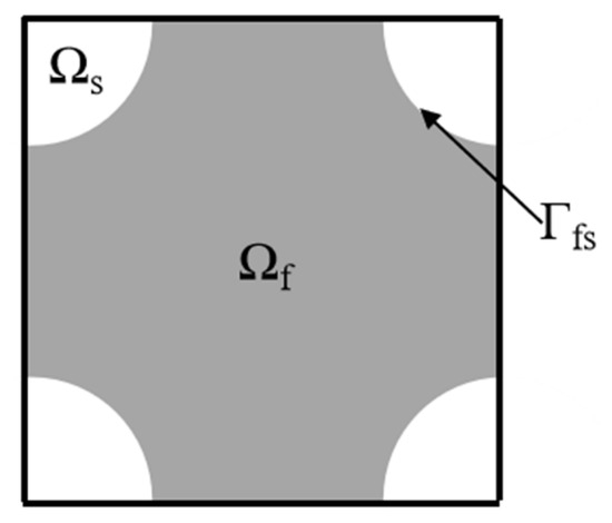
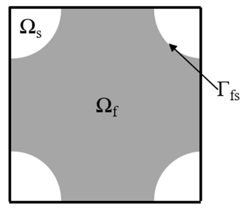
The square reference cell in Figure 2 has side length 3 and a circular solid inclusion of radius 1, giving $\phi =1-\pi /9\approx 0.6509$. Dimensional permeability is obtained from $K_{\mathrm{physical}}=l^2{K}_{\mathrm{dimensionless}}$ using the same reference length as in $\mathrm{Kn}$.

Figure 2. Schematic diagram of a periodic unit cell.

For a unit driving force $-{\nabla }_{x}p=e_x$ and zero gravity, solve the zero-slip cell problem for ${\omega }^0$. The superficial average of this velocity, multiplied by $\mu$, gives the first column of $K$:

$$K_{i1}=\mu {⟨{\omega }_i^0⟩}_{\mathrm{f}},\hspace{1em}i=1,2;\hspace{1em}-\nabla p=e_x,\hspace{1em}g=0$$

(65)

Square symmetry gives $K_{11}=K_{22}$ and $K_{12}=K_{21}=0$, within numerical error. The recursive cell problems supply the higher-order velocity and permeability coefficients.

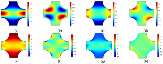
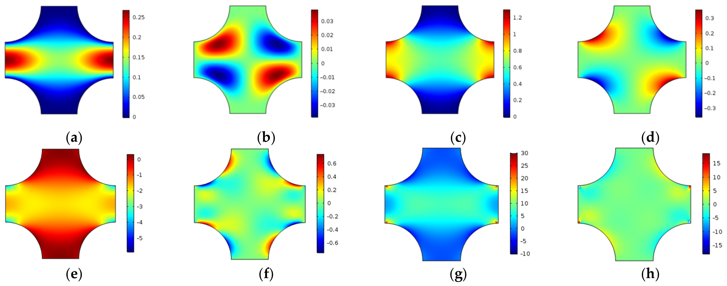
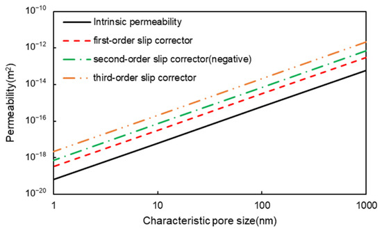
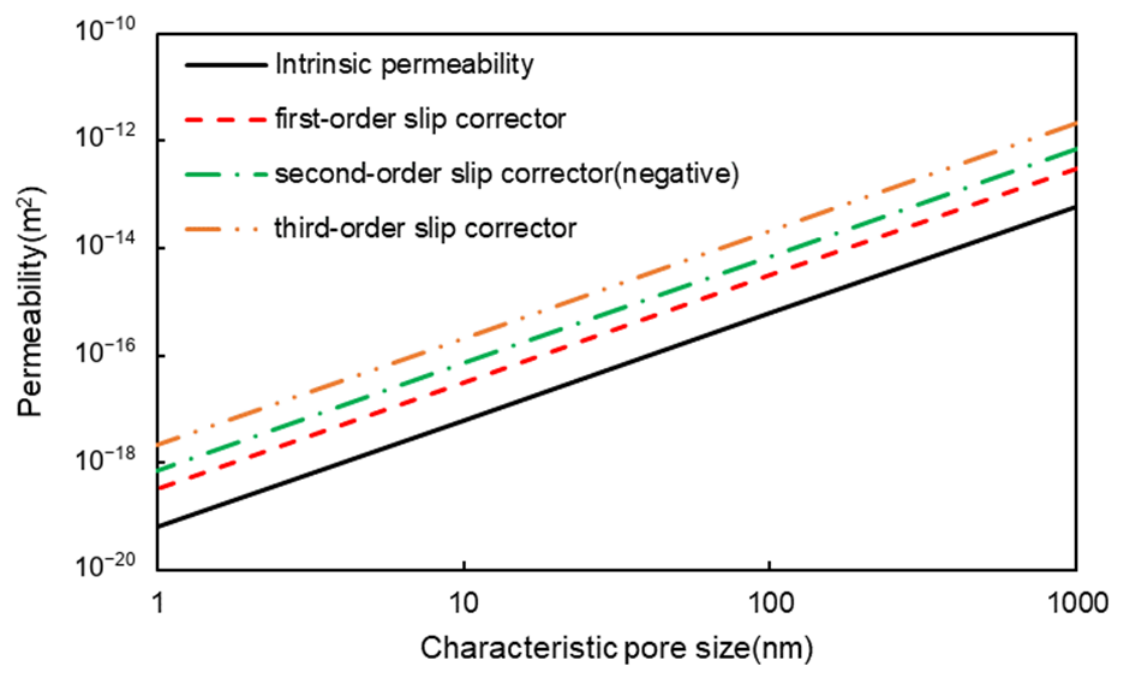
Figure 3 shows the coefficient fields ${\omega }^0$ through ${\omega }^3$, whose weighted sum gives the relative fluid velocity. Figure 4 exhibits the $l^2$ scaling of dimensional permeability for geometrically similar cells.

Figure 3. Dimensionless velocity coefficients under unit $x$-directed driving: (a) ${\omega }_x^0$, (b) ${\omega }_y^0$, (c) ${\omega }_x^1$, (d) ${\omega }_y^1$, (e) ${\omega }_x^2$, (f) ${\omega }_y^2$, (g) ${\omega }_x^3$, and (h) ${\omega }_y^3$. Each coefficient contributes ${\mathrm{Kn}}^n{\omega }^n$. Individual color ranges preserve spatial contrast in fields with different amplitudes; magnitudes are given by the corresponding color bars.

Figure 4. Permeability versus characteristic pore size.

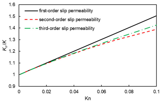
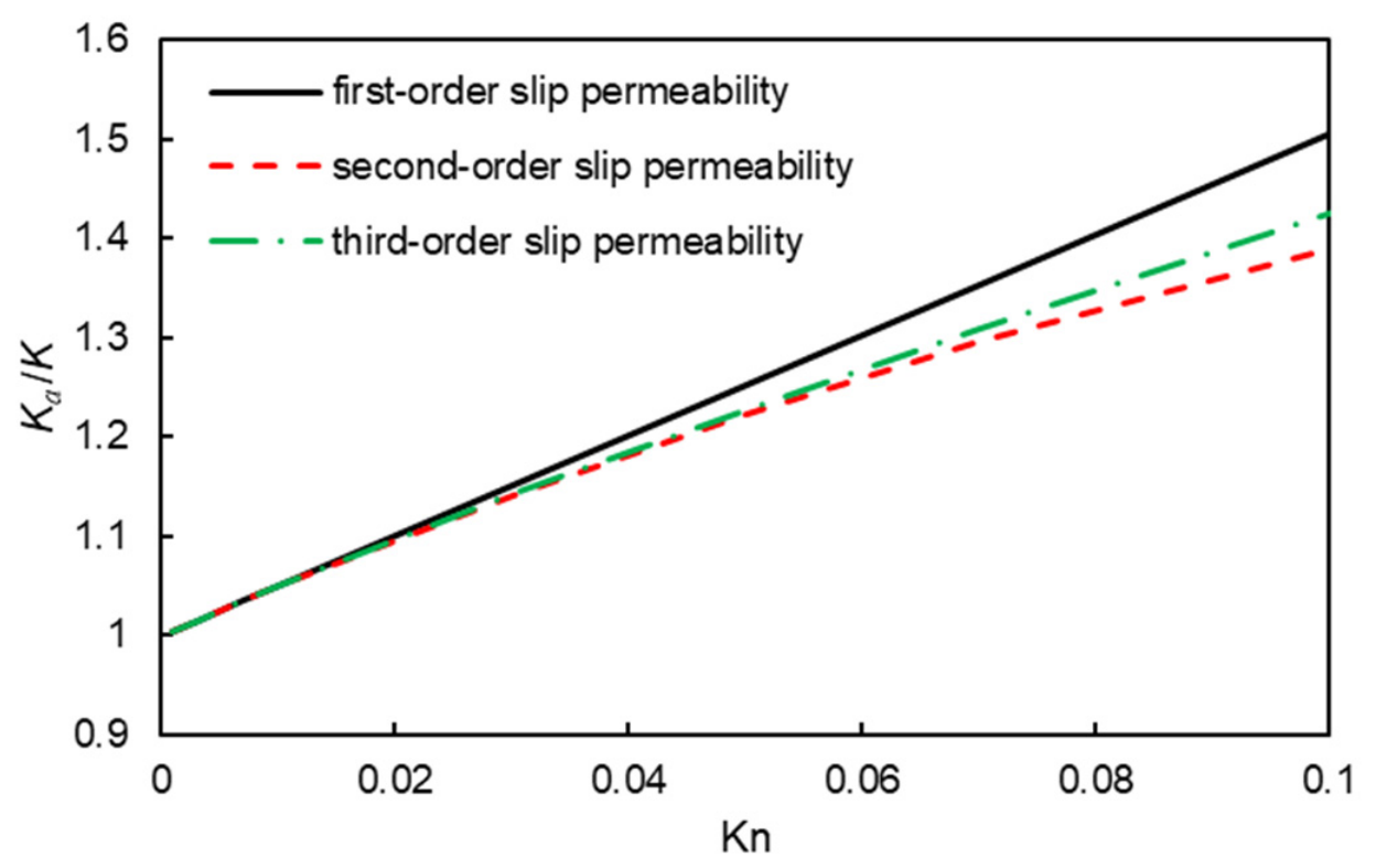
Figure 5 compares the first-, second-, and third-order approximations of $K_{\mathrm{a}}/K$. The second- and third-order terms modify the linear slip response in opposite directions for this geometry. Their separation increases with $\mathrm{Kn}$, showing the growing importance of truncation order.

Figure 5. $K_{\mathrm{a}}/K$ versus Knudsen number.

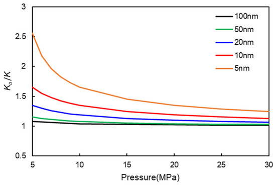
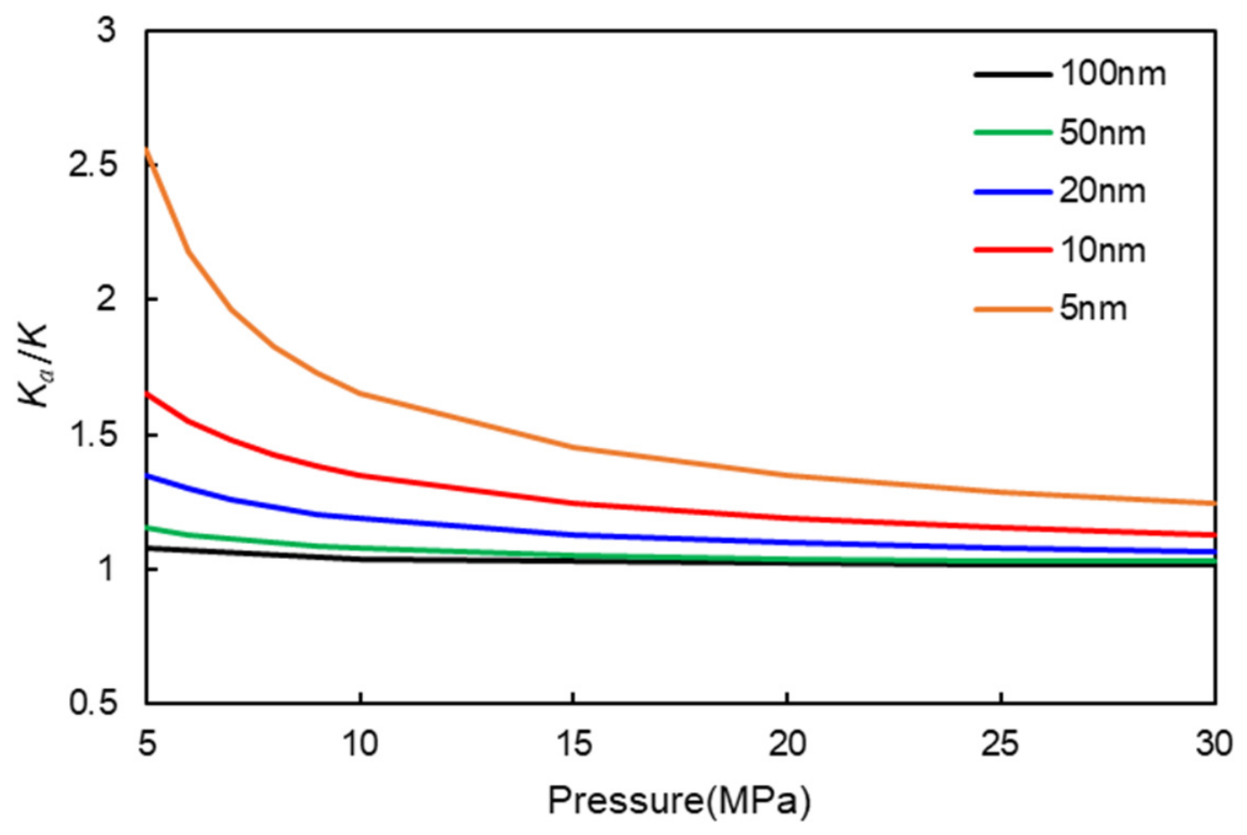
Figure 6 shows the pressure and pore-size dependence introduced by $\mathrm{Kn}=c\lambda /l$. With the hard-sphere estimate, $\mathrm{Kn}={\displaystyle \frac{c{k}_{\mathrm{B}}T}{\sqrt{2}\pi d^{2}pl}}$, so lower pressure or smaller pores increase the slip correction. Conversion to dimensional pressure and size depends on the gas, temperature, wall coefficient, and length convention.

Figure 6. $K_{\mathrm{a}}/K$ versus pore size and pressure.

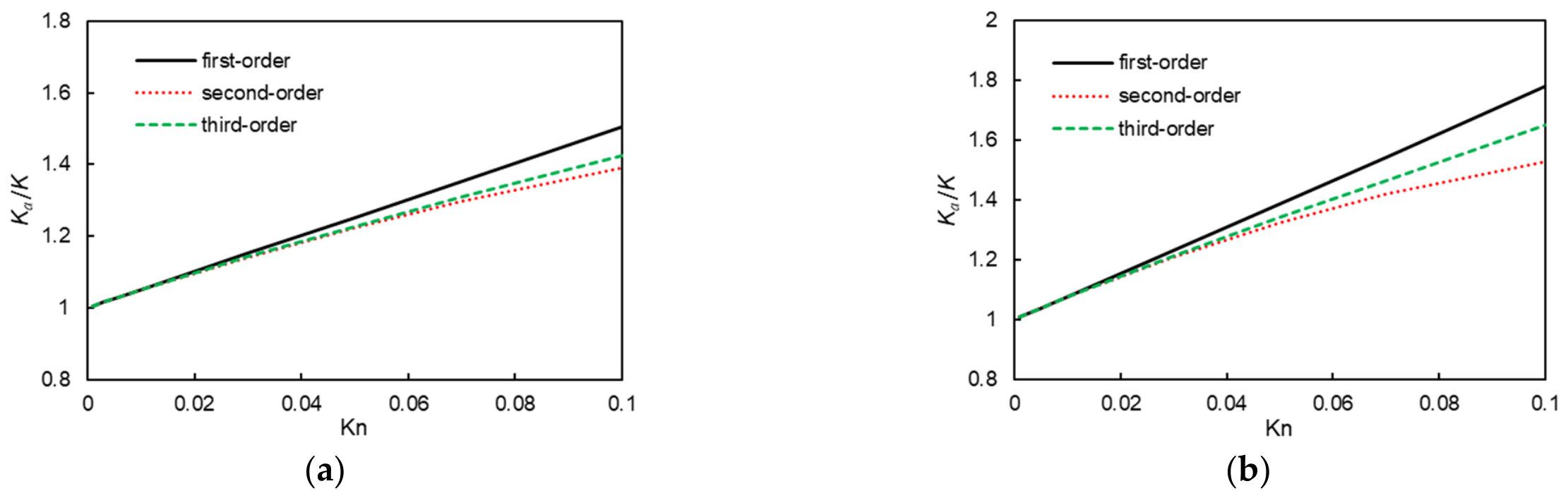
Figure 7, Figure 8 and Figure 9 compare four pore configurations with different interfacial-area descriptors. The permeability curves show stronger order sensitivity as the geometry changes toward more constricted flow paths. Since porosity, curvature, and throat dimensions vary together, the comparison characterizes the combined geometrical effect.

Figure 7. Two-dimensional comparison cells and their dimensionless interfacial-area descriptors $S_v$: (a) 0.523, (b) 0.785, (c) 0.942, and (d) 1.047.

Figure 8. Dimensionless $x$-directed velocity coefficients for the geometries of Figure 7, in the same row order. Columns (a–d) show ${\omega }_x^0$, ${\omega }_x^1$, ${\omega }_x^2$, and ${\omega }_x^3$. Each field contributes ${\mathrm{Kn}}^n{\omega }^n$. Individual ranges preserve spatial contrast across orders and geometries; averaged transport is compared in Figure 9.

Figure 9. First- to third-order approximations of $K_{\mathrm{a}}/K$ versus $\mathrm{Kn}$ for the 2D cells: (a) $S_v=0.523$, (b) 0.785, (c) 0.942, and (d) 1.047.

3.2. Three-Dimensional Particle Packings

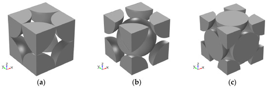
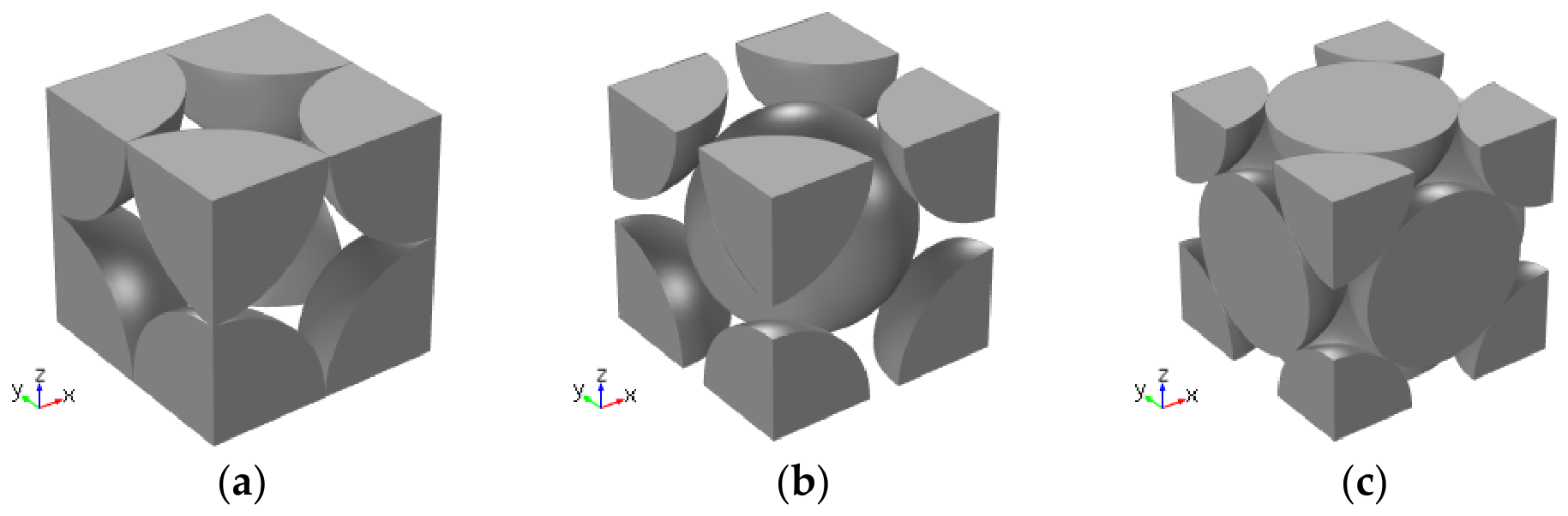
Three periodic particle arrangements are considered: simple cubic (C), body-centered cubic (BCC), and face-centered cubic (FCC) (Figure 10). The cell dimensions are $2\times 2\times 2$. Varying the equal particle radius within each arrangement changes porosity and solid-connection dimensions. The solid properties are $E/E_{\mathrm{ref}}=1$ and $\nu =0.3$.

Figure 10. Periodic particle packings: (a) C, (b) BCC, and (c) FCC.

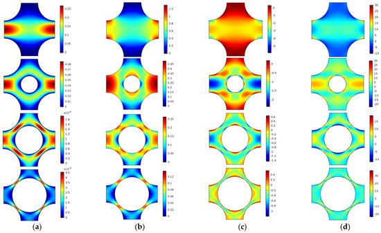
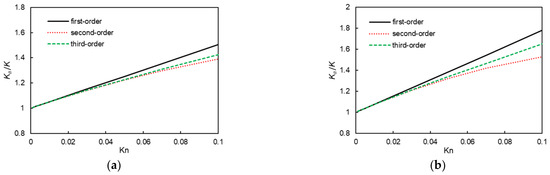
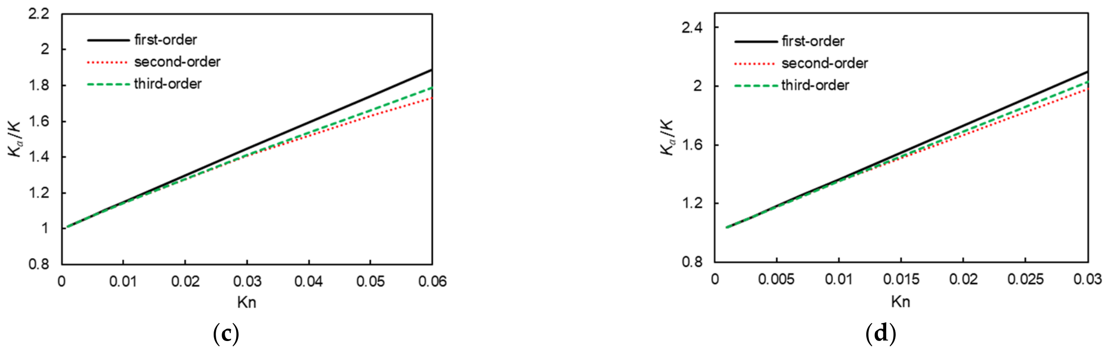
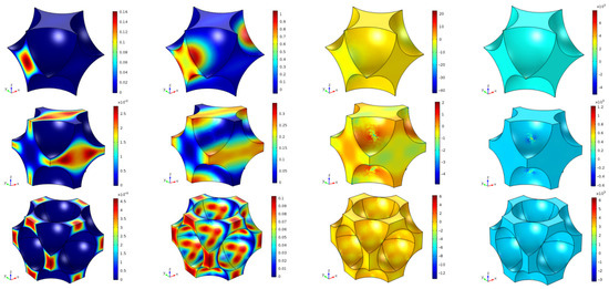
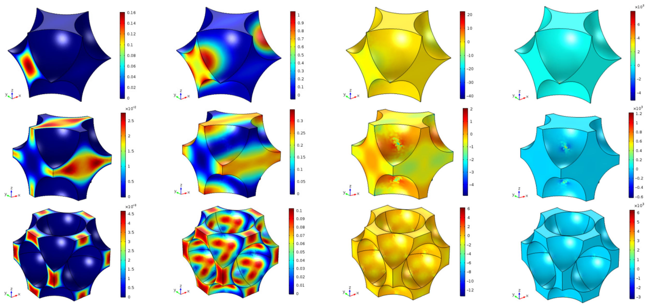
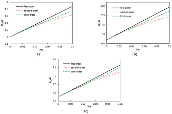
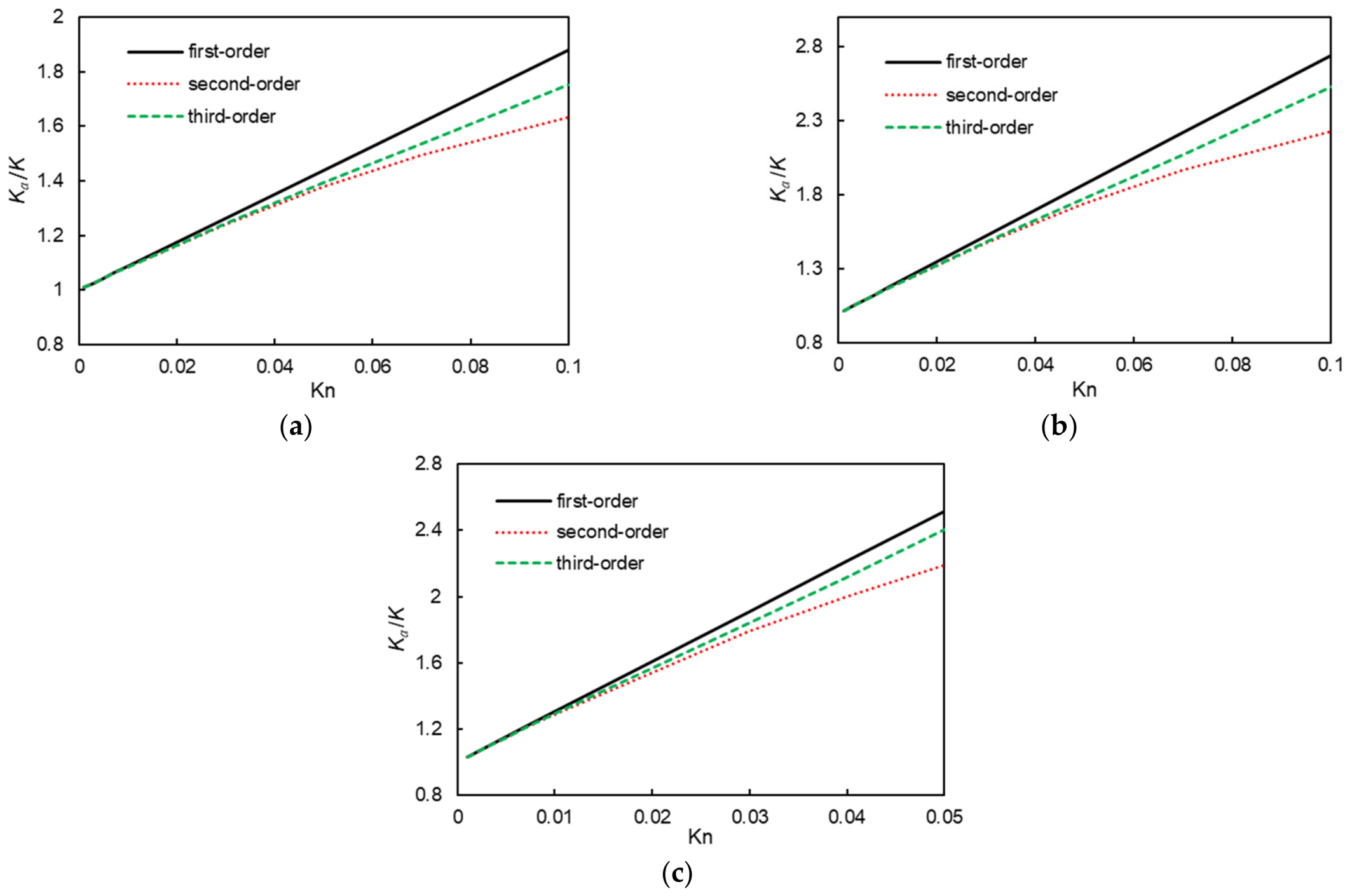
Figure 11 and Figure 12 show the $x$-directed velocity coefficients and permeability truncations for the three packings. Their distinct coefficient fields and order sensitivity reflect differences in the connected pore space and flow constrictions.

Figure 11. Dimensionless $x$ components ${\omega }_x^0$, ${\omega }_x^1$, ${\omega }_x^2$, and ${\omega }_x^3$ in columns (a–d), with C, BCC, and FCC cells from top to bottom. The driving is $x$-directed and the color ranges are individual to each coefficient field.

Figure 12. First- to third-order approximations of $K_{\mathrm{a}}/K$ for (a) C, (b) BCC, and (c) FCC cells.

The elastic and pressure-loading correctors define the effective stiffness and Biot tensor. These particle arrangements have cubic symmetry.

Solving Equations (25) and (27) for symmetric unit strains and unit pressure, respectively, and averaging by Equations (36) and (37) gives $c_{ijkl}$ and ${\alpha }_{ij}$. The cubic stiffness takes the form of Nunan and Keller [42]:

$$c_{ijkl}=\widehat{\lambda }\left(1+A\right){\delta }_{ij}{\delta }_{kl}+\widehat{\mu }\left(1+B\right)\left({\delta }_{ik}{\delta }_{jl}+{\delta }_{il}{\delta }_{jk}\right)+2\widehat{\mu }\left(C-B\right){\delta }_{ijkl}$$

(66)

Here ${\delta }_{ijkl}=1$ when $i=j=k=l$ and zero otherwise. The geometry-dependent factors $A$, $B$, and $C$ define three independent cubic stiffnesses. In the tensor convention ${\sigma }_{ij}=c_{ijkl}{e}_{kl}$, these are

$$c_{1111}=c_{2222}=c_{3333}=\widehat{\lambda }\left(1+A\right)+2\widehat{\mu }\left(1+C\right)={\widehat{\lambda }}_e+2{\widehat{\mu }}_{e2}$$

(67)

$$c_{1122}=c_{1133}=c_{2233}=c_{2211}=c_{3311}=c_{3322}=\widehat{\lambda }\left(1+A\right)={\widehat{\lambda }}_e$$

(68)

$$c_{1212}=c_{1313}=c_{2323}={\mu }_s(1+B)=C_{44}$$

(69)

Set $C_{11}=c_{1111}$, $C_{12}=c_{1122}$, and $C_{44}=c_{1212}$. The three cubic stiffnesses are independent. Young’s modulus and transverse Poisson’s ratio along a cubic axis are

$$E_{[100]}={\displaystyle \frac{(C_{11}-C_{12})(C_{11}+2C_{12})}{C_{11}+C_{12}}}$$

(70)

$${\nu }_{[100]}={\displaystyle \frac{C_{12}}{C_{11}+C_{12}}}$$

(71)

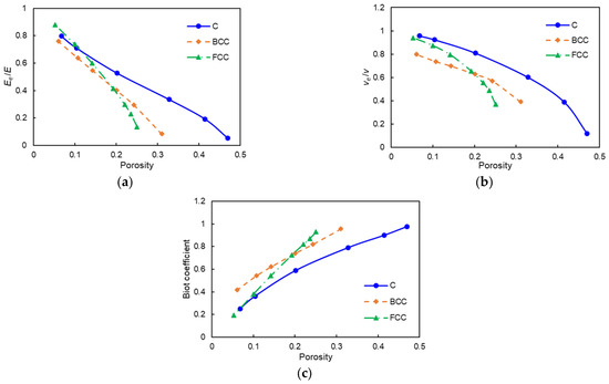
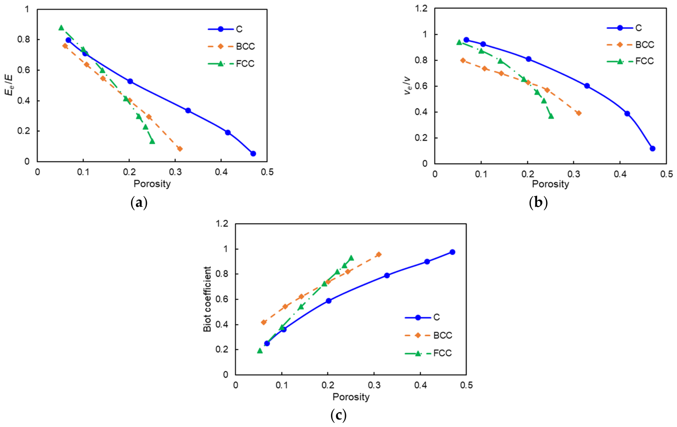
Figure 13 shows increasing stiffness and decreasing pressure coupling as the solid fraction increases. The growth of finite-area solid connections strengthens the load paths. $E_{[100]}$ and ${\nu }_{[100]}$ characterize the axial response; the independent shear stiffness $C_{44}$ completes the cubic description. At a point-contact endpoint, loss of finite-area connections can make the elastic response degenerate.

Figure 13. Elastic properties of the cubic cells versus porosity: (a) $E_{[100]}/E_{\mathrm{ref}}$, (b) ${\nu }_{[100]}/\nu$, and (c) diagonal Biot coefficient ${\alpha }_{ii}$. $E_{[100]}$ and ${\nu }_{[100]}$ describe loading along a cubic axis.

3.3. Periodic Capillary Cell

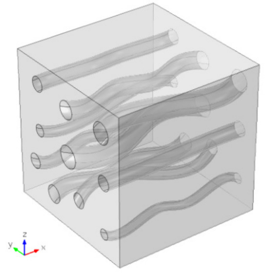
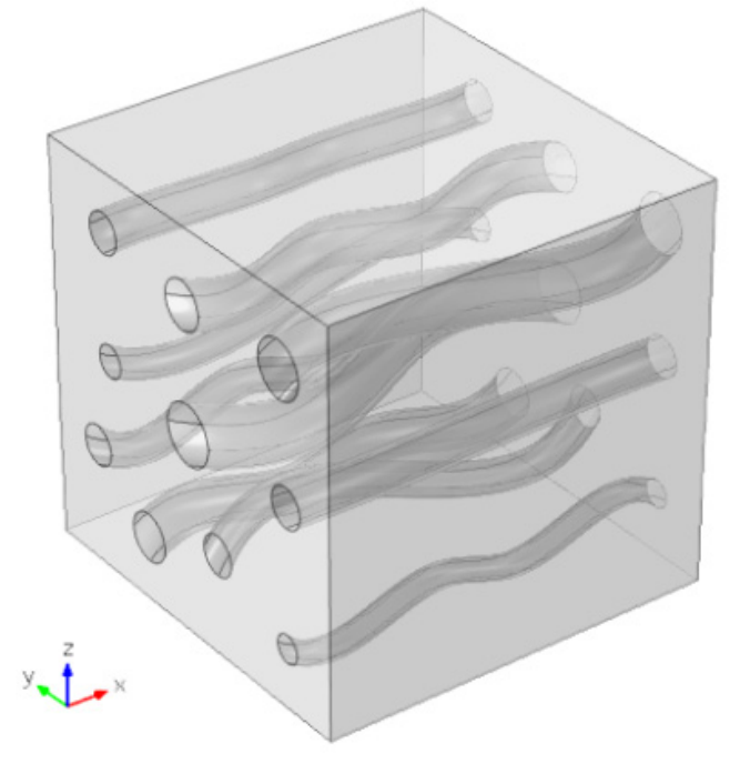
Figure 14 shows a prescribed capillary cell of dimensions $1\times 1\times 1$, with solid properties $E/E_{\mathrm{ref}}=1$ and $\nu =0.3$. Ten slender, smoothly curved channels are predominantly aligned with the $x$-direction; direct CAD measurement gives ten circular inlet openings with radii 0.035–0.075. The retained construction uses circular profiles swept along interpolation curves and subtracted from a cube. The example illustrates the directional response of a prescribed pore structure rather than an ensemble average or an established statistical REV.

Figure 14. Periodic capillary geometry. Opposite outer faces are paired; ${\mathsf{\Gamma }}_{\mathrm{fs}}$ is the internal gas–solid interface.

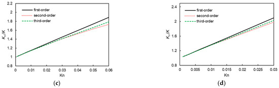
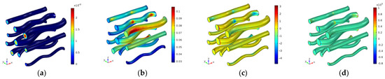
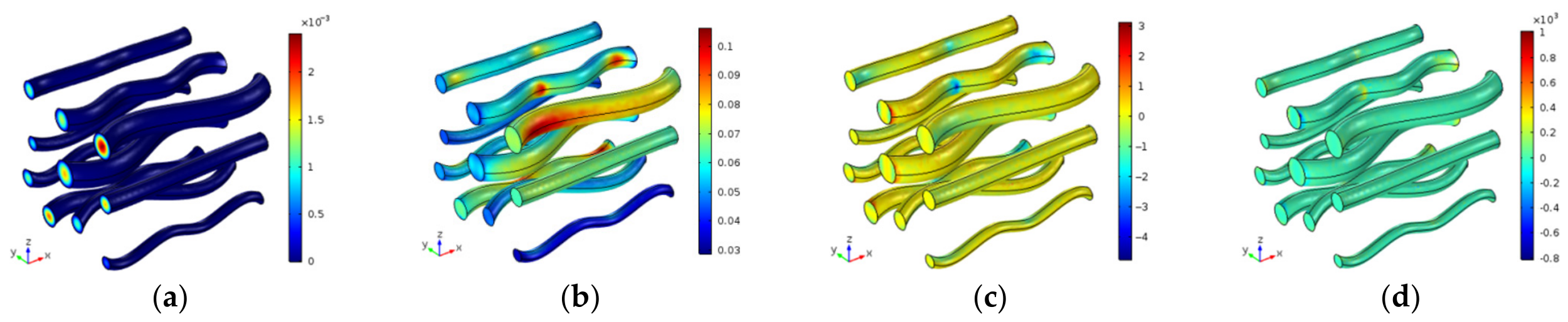
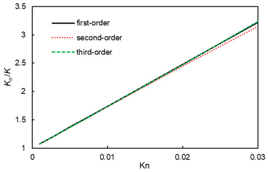
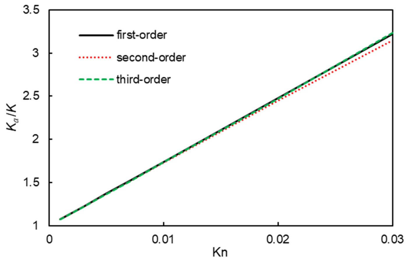
The velocity coefficients are shown in Figure 15. Figure 16 compares the first three permeability truncations over $\mathrm{Kn}=0.001–0.03$. The third-order increment $s_3$ is 0.191% at $\mathrm{Kn}=0.01$ and 2.76% at $\mathrm{Kn}=0.03$, quantifying the separation between retained orders within the plotted interval.

Figure 15. Dimensionless $x$ components of the capillary-cell velocity coefficients under unit $x$-directed driving: (a) ${\omega }_x^0$, (b) ${\omega }_x^1$, (c) ${\omega }_x^2$, and (d) ${\omega }_x^3$. Each field contributes ${\mathrm{Kn}}^n{\omega }^n$ and uses its displayed color range.

Figure 16. First- to third-order approximations of $K_{\mathrm{a}}/K$ versus $\mathrm{Kn}$ over 0.001–0.03 in the capillary cell.

Table 2 reports selected normal stiffnesses and diagonal Biot coefficients. Their directional differences describe the response of this cell. Cross and shear components are omitted from the table without being assumed zero; the cubic-axis Formulas (70) and (71) are not applied to this geometry.

Table 2. Selected stiffness components $c_{iiii}/E_{\mathrm{ref}}$ and dimensionless Biot coefficients ${\alpha }_{ii}$ for the capillary cell. The solid has $E_{\mathrm{ref}}=1 \mathrm{GPa}$ and $\nu =0.3$; all averages use the whole cell volume. The coefficient post-processing uses a solid fraction of 0.91937, giving $\phi =0.08063$; direct measurement of the retained capillary CAD gives $\phi =0.080607$.

${\mathbf{c}}_{1111}/{\mathbf{E}}_{\mathbf{r}\mathbf{e}\mathbf{f}}$	${\mathbf{c}}_{2222}/{\mathbf{E}}_{\mathbf{r}\mathbf{e}\mathbf{f}}$	${\mathbf{c}}_{3333}/{\mathbf{E}}_{\mathbf{r}\mathbf{e}\mathbf{f}}$	${\mathbf{\alpha }}_{11}$	${\mathbf{\alpha }}_{22}$	${\mathbf{\alpha }}_{33}$
1.1630	1.0376	1.0586	0.18436	0.24205	0.23176

For the adopted solid properties, ${\lambda }_s/E_{\mathrm{ref}}=0.576923$ and ${\mu }_s/E_{\mathrm{ref}}=0.384615$, giving $a_{1111}/E_{\mathrm{ref}}=1.346154$ as the dense-solid reference.

3.4. Analytical and Numerical Consistency Checks

Mesh sensitivity is evaluated for the effective coefficients themselves, using ${\eta }_Q=100\left|Q_{\mathrm{fine}}-Q_{\mathrm{previous}}\left|/\right|Q_{\mathrm{fine}}\right|$. Table 3 reports the three finest meshes of a seven-level 2D sequence and three meshes for the C-type 3D flow cell. For 2D, the global maximum/minimum sizes are $0.105f/0.003f$ and the wall sizes are $0.039f/0.00045f$, with $f=1, 0.7, 0.5, 0.35, 0.25, 0.18, 0.125$. For 3D flow, the corresponding sizes are $0.2f/0.06f$ and $0.106f/0.02f$, with $f=1, 0.7, 0.5$. All sizes are in the retained cell-coordinate units. The direct 3D calculation holds the dimensionless Navier slip length $b/l=0.1$ fixed during refinement, avoiding a slip length tied to the mesh size.

Table 3. Mesh refinement for effective permeability. The 2D quantity is the third-order sum $K_{\mathrm{a}}^{(3)}$ at $\mathrm{Kn}=0.1$; the 3D quantity is the direct, unexpanded Navier-slip solution at $b/l=0.1$. Permeabilities are normalized by $l^2$. DOF denotes the active degrees of freedom, excluding internal variables.

Cell	Elements	DOF	${\mathbf{K}}^0/{\mathbf{l}}^2$	${\mathbf{K}}_{\mathbf{a}}/{\mathbf{l}}^2$
2D	33,988	212,772	0.061264773	0.08783794
2D	61,048	378,516	0.061253136	0.087838744
2D	117,818	724,440	0.061258868	0.087881671
3D C	29,397	30,184	0.0096117086	0.016188546
3D C	63,973	60,756	0.0096872845	0.016483596
3D C	149,670	133,320	0.0096215928	0.01655084

Between the two finest 2D meshes, $K_{\mathrm{a}}^{(3)}$ changes by 0.0488% at $\mathrm{Kn}=0.1$; the individual $K^0$, $K^1$, $K^2$, and $K^3$ changes are 0.00936%, 0.151%, 0.261%, and 0.384%, respectively. For the direct 3D solution, the corresponding changes in $K_{\mathrm{a}}$, $K^0$, and $K_{\mathrm{a}}/K^0$ are 0.406%, 0.683%, and 1.08%. These are adjacent-mesh sensitivity measures rather than certified errors relative to an exact complex-cell solution. The newly refined 2D $K_{\mathrm{a}}^{(3)}$ at $\mathrm{Kn}=0.1$ differs from the archived value by 0.0222%, and its enhancement ratio differs by about 0.74%. Individual archived coefficients can differ by up to 4.77%, so this comparison does not assign the new convergence rates to the archived coefficient set.

A separate three-level test of the C-cell corrector hierarchy gives the last adjacent changes in $K_{\mathrm{a}}^{(3)}$ of 0.297% at $\mathrm{Kn}=0.03$ and 3.80% at $\mathrm{Kn}=0.1$. Successive correctors transfer wall-gradient data from the preceding order, making individual higher-order coefficients a more demanding discretization check than the weighted total permeability. Mesh independence of the individual 3D higher-order coefficients has not been established; the retained 3D curves are therefore interpreted as comparisons of truncation sensitivity.

For the C-type elastic model, global maximum/minimum mesh sizes are reduced from 0.16/0.02 to 0.128/0.016 and 0.1024/0.0128, with the remaining meshing controls fixed. Unit 11 strain and unit pore-pressure loads give the results in Table 4. Between the last two meshes, $c_{1111}/E_{\mathrm{ref}}$ change by 0.228% and ${\alpha }_{11}$ by 0.0102%; the independent strain/pressure reciprocity calculation of ${\alpha }_{11}$ differs by at most $1.46\times {10}^{-6}$ in absolute value over this sequence.

Table 4. Mesh refinement for the C-type elastic cell with $E_{\mathrm{ref}}=1 \mathrm{GPa}$ and $\nu =0.3$. DOF excludes one internal variable.

Elements	DOF	${\mathbf{c}}_{1111}/{\mathbf{E}}_{\mathbf{r}\mathbf{e}\mathbf{f}}$	${\mathbf{\alpha }}_{11}$
30,891	167,355	0.053083393	0.9772471
55,010	251,637	0.05292432	0.97732821
93,672	415,878	0.052803865	0.97742755

The finest-mesh reported linear residuals (LinRes) are $5.4\times {10}^{-9}$ for 2D flow, $5.2\times {10}^{-14}$ for direct 3D slip flow, and $4.9\times {10}^{-14}/3.4\times {10}^{-14}$ for the 3D strain/pressure loads. These residuals describe the algebraic solves and are distinct from the mesh sensitivities above.

Exact straight-channel solutions provide reference limits for the slip closure. For a slit of half-width $h$, slip length $b=c\lambda$, and driving $G_x=-dp/dx$, $u(y)=G_x(h^2-y^2+2bh)/(2\mu )$. The superficial permeability is $K_0=\phi h^2/3$ and $K_a/K_0=1+3b/h$. For a circular tube of radius $R$, $u(r)=G_x(R^2-r^2+2bR)/(4\mu )$, $K_0=\phi R^2/8$, and $K_a/K_0=1+4b/R$. Both ratios are linear in the appropriate slip parameter, so the higher coefficients vanish in these straight-channel limits. An additional finite-element slit calculation with $h=1$, $\mu =1$, $G_x=1$, 1534 triangular elements, quadratic velocity interpolation, and stationary tolerance ${10}^{-8}$ gives $K_a/K_0=1.000000, 1.030000, 1.300000$ at $b/h=0, 0.01, 0.1$. Relative errors against the analytical values are below ${10}^{-10}$; the exact parabolic profile lies in the quadratic velocity space. This benchmark checks the wall-law implementation and permeability normalization, independently of the complex-cell mesh studies.

The elastic closure satisfies reciprocal-work symmetry and the drained-void energy bound $E:c:E\le (1-\phi )E:a:E$ for any symmetric test strain $E$. Stability requires positive energy for nonzero $E$; for cubic symmetry the conditions are $C_{44}>0$, $C_{11}-C_{12}>0$, and $C_{11}+2C_{12}>0$. A numerical assessment of these conditions uses the full stiffness tensor and the geometric porosity.

For the retained capillary stiffness matrix, the relative major-symmetry discrepancy $\Vert C-C^{\mathrm{T}}{\Vert }_F/\Vert C{\Vert }_F$ is $6.40\times {10}^{-4}$. In engineering-shear Voigt notation (11, 22, 33, 12, 23, 31), its symmetric energy part $C_s=(C+C^{\mathrm{T}})/2$ has a minimum eigenvalue of $0.306596E_{\mathrm{ref}}$. Using the solid fraction in Table 2, $(1-\phi )A-C_s$ is also positive definite, with minimum eigenvalue $0.0143692E_{\mathrm{ref}}$, where $A$ is the constituent stiffness in the same notation. The pressure-loading Biot entries agree with ${\alpha }_{ij}={\delta }_{ij}-c_{ijkk}/(3K_s)$ to within $3.7\times {10}^{-4}$ in absolute value (0.16% relative), where $K_s$ is the bulk modulus of the isotropic solid. These checks use the retained unsymmetrized data; $C_s$ is used only to evaluate strain energy.

3.5. Discussion and Range of Application

The geometry comparisons link higher-order transport corrections to the organization of the pore space. At $\mathrm{Kn}=0.03$, $s_3$ is 0.263%, 0.554%, 2.56%, and 2.76% for C, BCC, FCC, and the capillary example, respectively. At the upper plotted $\mathrm{Kn}$ values it reaches 6.93% for C and 12.0% for BCC at $\mathrm{Kn}=0.1$, and 9.07% for FCC at $\mathrm{Kn}=0.05$. The separation is therefore both geometry- and $\mathrm{Kn}$-dependent. Interfacial area, porosity, curvature, and throat size change together in these cases, so the observations concern the complete geometries.

Gas and skeleton compressibility contribute differently to storage. The linear balance separates the gas term ${\phi }_0{\beta }_0\dot{\pi }$ from the elastic terms ${\rho }_0{\zeta }^{\prime }\dot{\pi }$ and ${\rho }_0\alpha :e({\dot{u}}_{\mathrm{s}})$. For an ideal gas, ${\beta }_0/{\rho }_0=1/p_0$, so lowering the reference pressure increases gas compliance and usually rarefaction. This is relevant to pressure depletion after a rapid drawdown. Application during fracture creation itself would require dynamic transport, evolving geometry, and damage beyond the quasi-static small-strain assumptions.

The range of the $\mathrm{Kn}$ expansion is also limited by the microscopic model. A first-order-slip continuum solution does not resolve the Knudsen layer [43]. Nominal $\mathrm{Kn}$ near 0.1, narrow throats, and strong order sensitivity therefore require kinetic assessment; no geometry-independent validity interval is established. Extrapolation to reservoir conditions can overestimate transport and production. Adsorption, surface diffusion, dense-gas corrections, and thermal effects require additional constitutive treatment.

The numerical examples illustrate geometry-dependent transport and elastic responses in prescribed cells. The mesh studies and tensor checks support the selected numerical quantities, while matched kinetic or experimental validation is needed for quantitative rock-scale prediction. The capillary example is interpreted as a prescribed pore structure rather than a statistical REV.

4. Conclusions

Two-scale homogenization yields a coupled description of compressible gas slip flow and small-strain poroelasticity. The main findings are:

(1)

The periodic transport closure gives geometry- and $\mathrm{Kn}$-dependent departures from the linear slip response. The existing coefficient sets quantify the separation between successive permeability truncations over the plotted ranges.

(2)

The elastic closure relates porosity and solid connections to effective stiffness and Biot coupling. The particle packings exhibit cubic response, and the selected capillary coefficients show directional differences.

(3)

Conservative mass transport separates gas-density storage from elastic pore-volume change. Its linearization recovers Biot-type storage and the rigid-matrix, incompressible-fluid, and no-slip limits.

The formulation applies to quasi-static, small-strain transport in the continuum slip regime. Quantitative use for a specified rock–gas system requires the numerical, kinetic, and structural verification discussed in Section 3.5.

References

- Karniadakis, G.; Beskok, A.; Aluru, N. Microflows and Nanoflows: Fundamentals and Simulation; Springer: New York, NY, USA, 2005. [Google Scholar]
- Cai, C.; Sun, Q.; Boyd, I.D. Gas flows in microchannels and microtubes. J. Fluid Mech. 2007, 589, 305–314. [Google Scholar] [CrossRef] [Scilit]
- Renu, K.; Kumar, A.; Negi, A.S.; Nimisha. Analytical analysis of magnetohydrodynamics mixed convection in a vertical microchannel in the presence of radiation. Multiscale Multidiscip. Model. Exp. Des. 2026, 9, 4. [Google Scholar] [CrossRef] [Scilit]
- Zhang, T.; Zhang, P.; Law, C.K.; Qi, F. CVD in weakly rarefied rotating disk flows. Chem. Vap. Depos. 2010, 15, 274–280. [Google Scholar] [CrossRef] [Scilit]
- Kolahdouz, M.; Salemi, A.; Moeen, M.; Östling, M.; Radamson, H.H. Kinetic modeling of low temperature epitaxy growth of SiGe using disilane and digermane. J. Electrochem. Soc. 2012, 159, H478–H481. [Google Scholar] [CrossRef] [Scilit]
- Wu, J.; Meng, X.; Ma, L.; Zhu, J.; Wang, Y.; He, L.; Li, X. Disilane synthesis by dielectric barrier discharge of gas-phase silane: Experimental test and computational simulation. Chem. Eng. Sci. 2025, 312, 121620. [Google Scholar] [CrossRef] [Scilit]
- Song, W.; Yao, J.; Li, Y.; Sun, H.; Zhang, L.; Yang, Y.; Zhao, J.; Sui, H. Apparent gas permeability in an organic-rich shale reservoir. Fuel 2016, 181, 973–984. [Google Scholar] [CrossRef] [Scilit]
- Sun, H.; Yao, J.; Cao, Y.C.; Fan, D.Y.; Zhang, L. Characterization of gas transport behaviors in shale gas and tight gas reservoirs by digital rock analysis. Int. J. Heat Mass Transf. 2017, 104, 227–239. [Google Scholar] [CrossRef] [Scilit]
- Afagwu, C.; Mahmoud, M.A.; Alafnan, S.; Patil, S. Multiscale storage and transport modeling in unconventional shale gas: A review. J. Pet. Sci. Eng. 2022, 208, 109518. [Google Scholar] [CrossRef] [Scilit]
- Darabi, H.; Ettehad, A.; Javadpour, F.; Sepehrnoori, K. Gas flow in ultra-tight shale strata. J. Fluid Mech. 2012, 710, 641–658. [Google Scholar] [CrossRef] [Scilit]
- Gao, Y.; Yu, Q. Experimental Study of the Effect of Molecular Collision Frequency and Adsorption Capacity on Gas Seepage Flux in Coal. SPE J. 2024, 29, 3293–3313. [Google Scholar] [CrossRef] [Scilit]
- Yang, D.; Jiang, C.; Wan, K.; Lee, C.H. Gas transport modeling in confined graphitic nanopores under high pressure. Int. J. Therm. Sci. 2026, 224, 110671. [Google Scholar] [CrossRef] [Scilit]
- Steckelmacher, W. Knudsen flow 75 years on: The current state of the art for flow of rarefied gases in tubes and systems. Rep. Prog. Phys. 1986, 49, 1083–1107. [Google Scholar] [CrossRef] [Scilit]
- Mokhtari, M.; Alqahtani, A.A.; Tutuncu, A.N.; Yin, X. Stress-dependent permeability anisotropy and wettability of shale Resources. In Proceedings of the Unconventional Resources Technology Conference, Denver, CO, USA, 12–14 August 2013; pp. 2713–2728. [Google Scholar]
- Katsuki, D.; Deben, A.P.; Adekunle, O.; Rixon, A.J.; Tutuncu, A.N. Stress-dependent permeability and dynamic elastic moduli of reservoir and seal shale. In Proceedings of the Unconventional Resources Technology Conference, San Antonio, TX, USA, 1–3 August 2016. [Google Scholar]
- Jiang, J.; Yang, J. Coupled fluid flow and geomechanics modeling of stress-sensitive production behavior in fractured shale gas reservoirs. Int. J. Rock Mech. Min. Sci. 2018, 101, 1–12. [Google Scholar] [CrossRef] [Scilit]
- Nwankwo, I.V.; Dejam, M.; Quillinan, S.A. A critical review of experimental and theoretical studies on shale geomechanical and deformation properties, fluid flow behavior, and coupled flow and geomechanics effects during production. Int. J. Coal Geol. 2025, 306, 104777. [Google Scholar] [CrossRef] [Scilit]
- Yang, Y.; Wu, W.; Zheng, H.; Wang, S.; Yang, L. An efficient monolithic multiscale numerical manifold model for fully coupled nonlinear saturated porous media. Comput. Methods Appl. Mech. Eng. 2024, 418, 116479. [Google Scholar] [CrossRef] [Scilit]
- Ho, C.K.; Webb, S.W. Gas Transport in Porous Media; Springer: Dordrecht, The Netherlands, 2006. [Google Scholar]
- Maxwell, J.C. On Stresses in Rarified Gases Arising from Inequalities of Temperature. Philos. Trans. R. Soc. Lond. 1879, 170, 231–256. [Google Scholar] [CrossRef] [Scilit]
- Deissler, R.G. An analysis of second-order slip flow and temperature-jump boundary conditions for rarefied gases. Int. J. Heat Mass Transf. 1964, 7, 681–694. [Google Scholar] [CrossRef] [Scilit]
- Beskok, A.; Karniadakis, G.E. A model for flows in channels, pipes, and ducts at micro and nano scales. Microscale Thermophys. Eng. 1999, 3, 43–77. [Google Scholar] [CrossRef] [Scilit]
- Song, W.; Yao, J.; Li, Y.; Sun, H.; Yang, Y. Fractal models for gas slippage factor in porous media considering second-order slip and surface adsorption. Int. J. Heat Mass Transf. 2018, 118, 948–960. [Google Scholar] [CrossRef] [Scilit]
- Dongari, N.; Agrawal, A. Modeling of Navier–Stokes equations for high Knudsen number gas flows. Int. J. Heat Mass Transf. 2012, 55, 4352–4358. [Google Scholar] [CrossRef] [Scilit]
- Zhang, T.; Jia, L.; Wang, Z. Validation of Navier–Stokes equations for slip flow analysis within transition region. Int. J. Heat Mass Transf. 2008, 51, 6323–6327. [Google Scholar] [CrossRef] [Scilit]
- Biot, M.A. General theory of three-dimensional consolidation. J. Appl. Phys. 1941, 12, 155–164. [Google Scholar] [CrossRef] [Scilit]
- Biot, M.A. Theory of elasticity and consolidation for a porous anisotropic solid. J. Appl. Phys. 1955, 26, 182–185. [Google Scholar] [CrossRef] [Scilit]
- Biot, M.A. Generalized theory of acoustic propagation in Porous Dissipative Media. J. Acoust. Soc. Am. 1962, 34, 1254–1264. [Google Scholar] [CrossRef] [Scilit]
- Burridge, R.; Keller, J.B. Poroelasticity equations derived from microstructure. J. Acoust. Soc. Am. 1981, 70, 1140–1146. [Google Scholar] [CrossRef] [Scilit]
- Chen, Z.; Lyons, S.L.; Qin, G. The mechanical behavior of a poroelastic medium saturated with a Newtonian fluid. Int. J. Numer. Anal. Model. 2004, 1, 75–97. [Google Scholar] [CrossRef] [Scilit]
- Xu, Z.; Zhang, J.; Young, Y.N.; Yue, P.; Feng, J.J. Comparison of four boundary conditions for the fluid-hydrogel interface. Phys. Rev. Fluids 2022, 7, 093301. [Google Scholar] [CrossRef] [Scilit]
- Skjetne, E.; Auriault, J.L. Homogenization of wall-slip gas flow through porous media. Transp. Porous Media 1999, 36, 293–306. [Google Scholar] [CrossRef] [Scilit]
- Foster, J.M.; Galvis, A.F.; Protas, B.; Chapman, S.J. Multiple scales homogenisation of a porous viscoelastic material with rigid inclusions: Application to lithium-ion battery electrodes. J. Mech. Phys. Solids 2025, 199, 106072. [Google Scholar] [CrossRef] [Scilit]
- Bouhlel, M.; Jamei, M.; Geindreau, C. Microstructural effects on the overall poroelastic properties of saturated porous media. Model. Simul. Mater. Sci. Eng. 2010, 18, 045009. [Google Scholar] [CrossRef] [Scilit]
- Lasseux, D.; Valdés-Parada, F.J.; Porter, M.L. An improved macroscale model for gas slip flow in porous media. J. Fluid Mech. 2016, 805, 118–146. [Google Scholar] [CrossRef] [Scilit]
- Lasseux, D.; Valdés-Parada, F.J.; Bottaro, A. Upscaled model for unsteady slip flow in porous media. J. Fluid Mech. 2021, 923, A37. [Google Scholar] [CrossRef] [Scilit]
- Lasseux, D.; Zaouter, T.; Valdés-Parada, F.J. Determination of Klinkenberg and higher-order correction tensors for slip flow in porous media. Phys. Rev. Fluids 2023, 8, 053401. [Google Scholar] [CrossRef] [Scilit]
- Garg, A. Enhanced flow in deformable carbon nanotubes. J. Appl. Phys. 2024, 135, 074304. [Google Scholar] [CrossRef] [Scilit]
- Mishra, H.; Garg, A. Heuristic modeling of material properties in Nano/Angstrom-scale channels: Integrating experimental observations and MD simulations. Microfluid. Nanofluidics 2025, 29, 14. [Google Scholar] [CrossRef] [Scilit]
- Auriault, J.L.; Strzelecki, T.; Bauer, J.; He, S. Porous deformable media saturated by a very compressible fluid: Quasi- statics. Eur. J. Mech. A Solids 1990, 9, 373–392. [Google Scholar]
- Nedjar, B. Formulation of a nonlinear porosity law for fully saturated porous media at finite strains. J. Mech. Phys. Solids 2013, 61, 537–556. [Google Scholar] [CrossRef] [Scilit]
- Nunan, K.C.; Keller, J.B. Effective elasticity tensor of a periodic composite. J. Mech. Phys. Solids 1984, 32, 259–280. [Google Scholar] [CrossRef] [Scilit]
- Wu, L.; Ho, M.T.; Germanou, L.; Gu, X.J.; Liu, C.; Xu, K.; Zhang, Y. A comment on “An improved macroscale model for gas slip flow in porous media”. arXiv 2017, arXiv:1702.04102. [Google Scholar] [CrossRef] [Scilit]
Disclaimer/Publisher’s Note: The statements, opinions and data contained in all publications are solely those of the individual author(s) and contributor(s) and not of MDPI and/or the editor(s). MDPI and/or the editor(s) disclaim responsibility for any injury to people or property resulting from any ideas, methods, instructions or products referred to in the content. |
© 2026 by the authors. Licensee MDPI, Basel, Switzerland. This article is an open access article distributed under the terms and conditions of the Creative Commons Attribution (CC BY) license.