


Abstract
Against the backdrop of the dual carbon goals of carbon peaking and carbon neutrality and the increasing penetration of renewable energy, conventional hierarchical planning methods for transmission and distribution networks are becoming insufficient to accurately characterize power exchange, boundary-voltage feasibility, and reserve support at the point of common coupling (PCC). This may lead to mismatches between distribution-side generation–storage planning decisions and actual system operating boundaries. To address this issue, this paper proposes a coordinated planning method for distribution-side distributed PV generation and energy storage that accounts for transmission–distribution coupling. First, the PCC is modeled as the physical interface between the transmission and distribution networks, and power-exchange balance, boundary-voltage feasibility, and interface-capacity constraints are introduced to transform traditionally exogenous boundary conditions into endogenous constraints. Then, a multi-objective planning model is developed to minimize annualized investment cost, operating cost, and PV curtailment rate, while considering transmission-network power flow, distribution-network voltage constraints, line-capacity limits, energy-storage state of charge, charging/discharging restrictions, and reserve-margin requirements jointly determined by allowable deviations in PV output and load demand. Finally, to address the computational burden caused by the nesting of multi-objective planning and full-year coordinated transmission–distribution operational verification, a hierarchical solution framework tailored to the model structure is developed. The outer-layer MOEA/D searches for PV–ESS capacity configurations, the middle-layer surrogate model screens candidate solutions requiring exact evaluation, and the inner-layer ADMM coordinates PCC boundary variables between the transmission and distribution sides, thereby obtaining a Pareto solution set that satisfies cross-level operating constraints. The results of an 8760 h case study on a typical regional power system show that compared with the conventional hierarchical planning scheme, the proposed method reduces the PV curtailment rate from 8.7% to 4.6%, increases PV utilization hours from 1160 h to 1375 h, reduces the peak power imported at the PCC from 8.2 MW to 6.5 MW, and reduces the total annualized system cost by 9.3%, while satisfying network-security and voltage constraints. The proposed method can quantitatively evaluate the comprehensive performance of alternative PV–ESS configurations in terms of PCC power exchange, distribution-network voltage constraints, and annual operating cost, thereby providing a planning tool for the siting and sizing of distribution-side PV and storage in regional grids with clearly defined transmission–distribution boundaries.
1. Introduction
The global transition toward low-carbon energy systems is reshaping the way power networks are planned and operated. As the share of solar and wind generation continues to rise, renewable variability is no longer confined to local balancing; it increasingly affects power flows, voltage conditions, and flexibility requirements across different network levels. The mismatch between renewable output and electricity demand may lead to transmission congestion, reverse power flow, voltage violations, and insufficient regulation capability [1,2,3]. Energy storage can ease some of these pressures by shifting energy across time and responding rapidly to changes in net load [4]. Its actual planning value, however, depends not only on installed capacity, but also on where the storage is connected and which network constraints are represented during planning.
Related integrated-energy-system planning studies account for carbon-trading price uncertainty [5] and multiple uncertainties through hybrid robust-interval optimization [6]. At the transmission-network level, a substantial body of research has examined the joint expansion of renewable generation, transmission facilities, and utility-scale storage. These studies seek to balance investment expenditure and operating costs while maintaining system-wide power balance and transmission security [7,8]. Renewable-generation uncertainty has also been incorporated through distributionally robust, adaptively robust, or scenario-based formulations [9,10,11]. These approaches are well suited to bulk-system planning, particularly when the main concern is the adequacy of generation and transmission capacity. Detailed conditions within active distribution networks, however, are commonly represented by aggregated loads or fixed nodal injections. As a result, feeder voltage limits, local hosting capacity, and the spatial allocation of distributed PV and storage are not fully captured.
A different line of research starts from the distribution network. A bi-level model has been proposed for the joint siting and sizing of distributed generation and energy storage in active distribution networks, linking investment decisions with storage operation [12]. Related tri-level research addresses energy-storage siting and sizing in transmission grids, together with multi-stage dispatch and market clearing under uncertainty [13]. Yi et al. [14] developed an active distribution-network expansion-planning model in which ESS deployment enhances network dispatchability. Lazo and Watts [15] formulated a stochastic active-distribution-network planning model to evaluate combinations of active network management schemes under uncertainty. Such models provide a more detailed account of voltage quality, feeder loading, network losses, and local renewable accommodation. The upstream grid, nevertheless, is often treated as an ideal slack source, a fixed electricity-price signal, or a prescribed exchange boundary. Under this assumption, the effect of distribution-side PV and storage decisions on upstream congestion and PCC loading remains only partly visible.
Research has gradually moved toward integrated or coordinated transmission–distribution planning. Existing studies have considered joint network expansion, hierarchical investment coordination, transmission-cost allocation, and decentralized planning with distributed-generation penetration [16,17,18,19]. A multi-stage stochastic framework has also been developed to co-optimize transmission and active-distribution investments under multidimensional uncertainty [20]. Related capacity-expansion research has also incorporated multi-timescale uncertainty and generation low-carbon retrofit into multi-period planning of regional integrated energy systems [21]. These contributions show that separate planning may produce inconsistent or economically inefficient decisions across network levels. Their emphasis, however, generally lies in network reinforcement, investment timing, or coordination of equivalent boundary information. The joint siting and sizing of distribution-side PV and energy storage when PCC power consistency, interface capacity, and distribution-side boundary-voltage feasibility are imposed at the same time has received less attention.
Table 1 compares representative studies from the above research streams. The comparison suggests that three issues remain open. First, PCC conditions are frequently prescribed in advance or represented through simplified exchange variables; they do not always enter the planning model as physical feasibility constraints. Second, coordinated transmission–distribution studies tend to focus on network assets, whereas the spatial allocation of distributed PV and storage is usually examined within the distribution network alone. Third, once annual operating conditions, cross-level power-flow limits, voltage constraints, and several planning objectives are considered together, the resulting problem becomes computationally demanding. An effective solution method therefore needs to preserve the physical connection between the two network levels without making every candidate planning scheme prohibitively expensive to evaluate.
Table 1.
Comparison of representative studies on renewable generation, energy storage, and transmission–distribution planning.
The distinction from the studies summarized in Table 1 is therefore not the use of a new generic optimization algorithm, but the planning object and the way transmission–distribution coupling enters the resource-allocation decision. Specifically, the proposed model uses PCC power consistency, interface capacity, and distribution-side voltage feasibility to directly influence the siting and sizing of distributed PV and ESSs, whereas the representative coordinated T–D studies in Table 1 mainly focus on network expansion, investment coordination, or equivalent boundary information. Against this background, the present study developed a coordinated planning method for distribution-side PV and energy storage under transmission–distribution coupling. The transmission and distribution networks are connected through multiple PCCs. Rather than fixing the interface conditions beforehand, the model evaluates each candidate configuration against transmission-network power-flow limits, PCC exchange and transformer-capacity constraints, distribution-network voltage and feeder limits, and the temporal operating characteristics of energy storage. The proposed method is subsequently examined using a representative regional transmission–distribution system, where distributed PV and storage are planned on the distribution side while the upstream network provides power-balancing and reserve support.
The main contributions are summarized as follows.
- (1)
- Endogenous integration of multidimensional PCC physical boundaries into distribution-side PV–ESS planning.
Unlike conventional transmission–distribution coordination methods that rely primarily on information exchange, equivalent boundary representations, or ex post feasibility checks, this study incorporates active-power consistency across both sides of the PCC, the apparent-power capacity of the interconnection transformer, and the feasibility of the distribution-side root-node voltage directly into the capacity-planning model. Consequently, transmission-side operating constraints can be fed back through the PCC to influence the siting and sizing of distribution-side PV and energy storage, while distribution-side resource allocation, in turn, affects transmission-network power flows and interface power exchange. This treatment constitutes the principal modeling contribution that distinguishes the proposed method from general hierarchical coordination frameworks.
- (2)
- Development of a multi-objective planning–operation closed-loop model for distribution-side resource allocation.
The model jointly determines the installed PV capacity, rated storage power, and rated storage energy capacity at candidate nodes, and verifies transmission-network power flow, distribution-network power flow, PCC boundary conditions, energy-storage operating states, and reserve margins over an 8760 h chronological operating horizon. Annualized investment cost, annual operating cost, and PV curtailment rate are used to characterize the trade-offs among resource investment, operational economy, and renewable-energy accommodation. The contribution does not lie merely in formulating a generic multi-objective model, but in enabling distribution-side resource-allocation decisions to be simultaneously verified against the operating boundaries of both the transmission and distribution networks.
- (3)
- Construction of a hierarchical solution framework tailored to the nested structure of the model.
The outer-layer MOEA/D searches for alternative PV–ESS capacity configurations, the middle-layer surrogate model screens candidate solutions requiring exact evaluation, and the inner-layer ADMM coordinates PCC boundary variables between the transmission- and distribution-side subproblems. This framework is designed to reduce the computational burden of annual operational verification while maintaining boundary consistency among the subproblems. Its contribution lies in the structure-specific integration of established algorithms with the proposed model, rather than in introducing new theoretical developments for MOEA/D, surrogate modeling, or ADMM.
This study integrated distribution-side PV and energy-storage capacity planning with full-year hourly steady-state operational verification. Transmission–distribution interactions were characterized through PCC power consistency, interface-capacity constraints, and distribution-side voltage constraints. The analysis focused on planning feasibility, renewable-energy accommodation, and economic performance under these modeling assumptions. Fault ride-through, transient rotor-angle stability, and voltage-collapse margin were outside the scope of this study.
2. A Hierarchical Coordinated Generation–Storage Planning Framework Considering PCC Physical Coupling and Boundary-Voltage Feasibility
2.1. Framework Description
With the increasing penetration of distributed renewable energy, the traditional hierarchical planning paradigm that treats transmission and distribution networks independently can no longer accurately represent physical interactions across network levels. In particular, power exchange at the point of common coupling (PCC), distribution-network voltage constraints, and system reserve requirements are strongly coupled with generation–storage planning decisions. Ignoring these interactions may lead to renewable-energy curtailment, insufficient flexibility, and infeasible operating conditions.
To address this issue, a coordinated generation–storage planning framework is established, as illustrated in Figure 1. The transmission and distribution networks are modeled as interconnected subsystems linked through the PCC. The transmission network is responsible for bulk power balancing, transmission-security assessment, and reserve provision, while the distribution network determines the siting and sizing of distributed renewable-energy generation and energy-storage systems (ESSs), subject to local operational constraints.
Figure 1.
Coordinated planning framework for distribution-side PV and energy storage considering PCC physical coupling, boundary-voltage feasibility, and reserve support.
Within the proposed framework, the PCC serves as the physical interface between the transmission and distribution networks. Instead of treating boundary conditions as fixed inputs, PCC power exchange is modeled as an endogenous variable jointly determined by transmission-network operating limits, distribution-network hosting capacity, and generation–storage regulation capability. Consequently, planning decisions are evaluated under realistic operating conditions.
In addition, the framework explicitly considers distribution-side boundary-voltage feasibility. The operational states of distributed PV, ESSs, and loads affect PCC power exchange and feeder voltage profiles, while transmission-side operating limits simultaneously influence renewable-energy accommodation capability. This bidirectional interaction enables coordinated evaluation of renewable-energy accommodation, network security, and operational feasibility.
To maintain operational flexibility under high PV penetration, the planning model further imposes upward and downward reserve-margin requirements. Rather than assuming probability distributions for PV and load forecast errors, the required upward and downward regulation capacities in each time period are determined using predefined deviations in PV output and load demand. Reserve support is jointly provided by conventional generators and distribution-side energy-storage systems. The reserve capability of conventional generators is constrained by their minimum and maximum output limits, whereas that of energy-storage systems is jointly limited by their rated power and current state of charge. Consequently, each planning scheme must not only satisfy power-balance and voltage constraints under the baseline annual chronological profiles, but also retain sufficient regulation margins to accommodate net-load deviations within a prescribed range.
2.2. PCC Definition and Physical Coupling Modeling
To explicitly characterize the physical coupling between the transmission network and the distribution network, the point of common coupling (PCC) is defined as the shared boundary between the two network models. Let PCC denote the set of PCCs, where PCC k is the electrical interface formed by the transmission–distribution interconnecting transformer, the connected transmission-side bus, and the root node of the distribution network. The transmission-side DC power-flow model and the distribution-side DistFlow model exchange boundary information through this interface.
PCC k performs three principal functions: it unifies the active-power representation of the same interface on both sides, verifies the capacity limit of the interconnecting transformer, and determines whether the distribution-side root-node voltage remains within the allowable range. To avoid ambiguity in the power-flow direction, and are defined as the active powers injected from PCC k into the transmission and distribution sides, respectively. When the distribution network imports power from the transmission network, , whereas . Therefore, the interface powers recorded by the two sides during the same time period must satisfy the conservation relationship in Equation (1):
where t is the operating-period index; k ∈ PCC denotes the kth transmission–distribution PCC; and and are the active powers injected from the PCC into the transmission and distribution sides, respectively, in MW. Equation (1) ensures that the two submodels produce consistent power values for the same physical interface.
In addition to active-power consistency, the rated capacity of the interconnecting transformer imposes a physical upper bound on boundary power exchange. Therefore, the active and reactive powers at the PCC must satisfy the apparent-power constraint in Equation (2):
where is the actual active-power exchange at PCC k and satisfies ; is the corresponding reactive-power exchange in Mvar; and is the rated capacity of the interconnecting transformer in MVA.
The net active power exchanged at the PCC on the distribution side is jointly determined by the nodal load, grid-connected PV output, ESS charging/discharging states, and the active-power losses of the distribution feeder connected to that PCC. Accordingly, Equation (3) is written as:
Here, denotes the aggregate active-power loss of the distribution feeder supplied through PCC k. For consistency with the linearized DistFlow formulation, it is evaluated using the branch-flow-based approximation, where is the set of distribution-network nodes supplied through PCC k; and are the active load and grid-connected PV power at node j, respectively; and and are the ESS discharging and charging powers, respectively, all in MW. Under the direction convention defined above, denotes the net power imported by the distribution area from the upstream transmission network.
Therefore, the distribution-side PCC power used for transmission–distribution coordination includes the same network-loss component as that used in the operating-cost calculation.
Because the transmission-side DC power-flow model does not include voltage-magnitude variables, voltage-magnitude equality is not imposed between the transmission and distribution sides. Instead, PCC voltage coordination is represented as a feasibility condition for the distribution-side root node: the boundary voltage calculated by the DistFlow model must remain within the allowable operating range, as expressed in Equation (5):
where is the voltage magnitude of the distribution-network root node connected to PCC k, in p.u.; and and are the allowable lower and upper voltage limits at that boundary node, respectively.
Through Equations (1)–(5), net-power variations caused by distribution-side loads, PV output, and ESS operation are transmitted to the transmission network through the PCC, thereby affecting transmission-line flows and conventional-generator outputs. Conversely, the PCC transformer-capacity limit and distribution-side boundary-voltage conditions constrain feasible PV and ESS configurations. The PCC therefore becomes an endogenous constraint linking planning decisions with operational verification at both network levels.
3. A Multi-Timescale Generation–Storage Planning Model for Transmission–Distribution Coordination
3.1. Modeling Framework
The increasing penetration of renewable energy has accelerated the transformation of distribution networks from traditional unidirectional supply systems into active distribution systems characterized by bidirectional power flows, strong output volatility, and high voltage sensitivity. In particular, large-scale integration of distributed PV generation may cause reverse power flow, voltage rise, branch-flow redistribution, and local accommodation constraints. Meanwhile, the transmission network is responsible not only for regional power balance and interconnection-capacity support, but also for providing boundary-voltage support, power-exchange channels, and reserve capacity to the distribution network through the point of common coupling (PCC). Therefore, the relationship between transmission and distribution networks is no longer a simple upper-level supply and lower-level consumption relationship, but a strongly coupled interaction involving power exchange, voltage feasibility, and flexible regulation capability at the PCC. If such coupling is neglected in planning, transmission–distribution boundary conditions are often simplified as fixed injection power, empirical margins, or parameters for ex post verification. As a result, planning schemes that appear feasible at the local distribution-network level may cause congestion in critical transmission sections, PCC capacity violations, distribution-network voltage-limit violations, and reduced renewable-energy accommodation under coordinated transmission–distribution operation.
To address the above issues, this study established a transmission–distribution coordinated planning model that considers PCC power coupling, distribution-side voltage feasibility, and reserve requirements. The framework forms a closed loop comprising capacity planning, operational verification, and boundary coordination. The capacity-planning layer determines PV capacity and ESS power and energy capacities at candidate distribution-network nodes; the operational-verification layer evaluates transmission power flow, distribution-network steady-state voltage, ESS charging/discharging, and PV accommodation over the full 8760 h chronology; and the boundary-coordination layer brings formerly exogenous interface conditions into the planning evaluation through PCC power conservation, distribution-side boundary-voltage feasibility, and interface-capacity constraints.
This study adopted a deterministic multi-period planning framework. Planning decisions were evaluated using given 8760 h PV-availability factors and load profiles; intraday PV variations, seasonal differences, and load peak-valley changes entered the operational verification through hourly input data. The annual chronology therefore captures representative operating variations over the planning horizon.
Beyond the baseline annual chronology, deterministic deviation bounds are used to represent net-load changes that may arise from short-term forecast errors. Upward reserve demand is induced by PV output below its forecast value and load above its forecast value, whereas downward reserve demand corresponds to PV output above its forecast value and load below its forecast value. These requirements preserve the necessary regulation margin for possible power deviations in each operating period. The case study further considers high-PV–low-load and low-PV–high-load stress scenarios to examine the adaptability of the selected planning schemes to input variations.
3.2. Multi-Objective Function
This paper formulates the integrated planning problem as a multi-objective coordinated optimization model considering investment cost, operating cost, and PV curtailment rate. Under high renewable-energy penetration, these objectives are strongly coupled. Minimizing investment may limit ESS deployment and reduce flexibility, whereas excessive curtailment reduction may cause overinvestment. Therefore, economic performance and renewable-energy accommodation must be balanced.
- (1)
- Minimizing investment costs
At the long-term planning level, annualized investment costs mainly include newly installed distributed PV capacity and the power and energy capacity of energy-storage systems. These costs reflect the capital expenditure of capacity decisions and serve as a key basis for evaluating the economic performance of the final planning scheme.
The unit investment coefficients used in Equation (6) are annualized equivalents of the corresponding initial capital costs. The conversion is performed using the capital-recovery factor:
where r is the annual discount rate and L is the economic lifetime of the corresponding asset. Accordingly, the annualized unit investment coefficient is obtained as cann = ccapCRF(r,L). PV capacity, ESS power-conversion capacity, and ESS energy capacity are annualized separately according to their respective economic lifetimes.
- (2)
- Minimizing operating costs
At the operational level, year-round operation incurs costs related to conventional generation in the transmission network, operation and maintenance of PV and energy-storage systems in the distribution network, network losses, and penalties for PV curtailment.
Specifically, is calculated from the aggregate distribution-network active-power loss defined in Equation (4). Thus, the loss term entering the operating-cost objective and the loss term included in the PCC power balance are evaluated using the same branch-flow results.
- (3)
- Minimizing the curtailment rate
In Equation (6), F1 is the annualized investment cost; is the planned PV capacity at candidate node n; and and are the rated power and rated energy capacity of the ESS at node e, respectively. , , and are the corresponding annualized unit investment costs, in CNY/(MW·year), CNY/(MW·year), and CNY/(MWh·year), respectively. In Equation (8), F2 is the annual operating cost and Δt is the duration of one operating period. , , , and denote the conventional-generation operating cost, PV and ESS O&M cost, network-loss cost, and PV-curtailment cost in period t, respectively. In Equation (9), and are the curtailed PV power and available PV power at node n in period t, respectively, and their ratio is used to calculate the annual PV-curtailment rate F3. Accordingly, the multi-objective vector in Equation (10) comprises annualized investment cost, annual operating cost, and annual PV-curtailment rate.
minF = [F1,F2,F3]
In the equation, the multi-objective vector F consists of investment cost, operating cost, and the curtailment rate.
3.3. Constraints
For a given generation–storage capacity configuration, the following constraints ensure power balance, network-capacity limits, steady-state voltage feasibility, and reserve adequacy over the annual chronological operation. Considering PV-output variation, intertemporal ESS coupling, transmission–distribution power flow, and PCC consistency, the constraints are organized around PV accommodation, ESS regulation, reserve support, network transfer, and boundary coupling. The scope of the security assessments included in this study is summarized in Appendix A, Table A1. In this study, reserve activation is associated with a net-load deviation from the baseline hourly operating point. Upward reserve is assumed to be called when actual PV output is lower than the baseline and/or actual load is higher than the baseline, whereas downward reserve is called for the opposite deviation. The deviation coefficients in Equations (38)–(39) specify the magnitude of the deviation that the scheduled reserve capacity is required to cover.
- (1)
- Renewable-energy output and curtailment constraints
To link planning decisions with operational performance, the relationship among installed PV capacity, available PV power, and grid-connected output is defined. Since PV output is driven by meteorological conditions, available PV power is determined by installed capacity and the time-varying generation factor rather than treated as an independent decision variable.
Due to local voltage constraints, branch-capacity limits, or PCC interface-capacity limits in the distribution network, the full available PV output cannot always be fed into the grid. Therefore, the available power must be allocated between actual grid-connected power and curtailed power.
To ensure that PV output decomposition is physically feasible, non-negativity and upper-bound constraints are imposed on actual grid-connected power and curtailed power so that neither exceeds the available power in the corresponding time slot.
Equations (11)–(16) describe the relationship between installed PV capacity and hourly output. is the PV-availability factor at node n in period t, and is the corresponding available PV power. and are the baseline or peak active loads at transmission node i and distribution node j, respectively, in MW; and are the corresponding hourly load factors. The available PV output is decomposed into actual grid-connected power and curtailed power ; both must be non-negative and cannot exceed the available PV power in the corresponding period.
- (2)
- Energy-Storage Operational Constraints
Energy storage is a key flexible regulation resource in the proposed model. Its role extends beyond energy time shifting and peak shaving to include mitigating PCC power fluctuations, suppressing local voltage violations, and providing reserve support.
The charging and discharging power of the energy-storage system at each time period is constrained by its planned rated power, ensuring consistency between capacity allocation and operational regulation capability.
To prevent simultaneous charging and discharging, binary charging and discharging state variables are introduced, with a mutual-exclusion constraint imposed to ensure physically consistent operation of the energy-storage system.
The dynamic behavior of the energy-storage system is characterized by the temporal evolution of the SOC, which is updated based on the previous SOC, current charging and discharging power, and the corresponding energy conversion efficiencies.
To prevent the energy-storage system from being overcharged or over-discharged, upper and lower limits must be imposed on the state of charge (SOC).
To avoid artificial energy transfer across the boundary of the annual scheduling horizon, the initial and terminal SOC conditions are explicitly imposed as:
Thus, each ESS starts from a prescribed initial SOC and is required to return to the same SOC after the complete 8760 h chronological simulation. This cyclic condition prevents the planning solution from obtaining an artificial operating benefit by depleting the stored energy at the end of the year.
Equations (17)–(22) jointly describe ESS operating constraints. and are the ESS charging and discharging powers, respectively, and are limited by the planned rated power . Binary variables and prevent simultaneous charging and discharging in the same period. SOCe,t is updated hourly according to the charging/discharging powers, efficiencies and , period duration Δt, and ESS energy capacity , and is maintained between and .
- (3)
- Transmission-network power flow constraints
At each transmission-network node, active power balance is maintained among conventional generation, local load, PCC power exchange, and line power flows. This constraint ensures transmission-network operational feasibility and links distribution-side generation–storage planning decisions with transmission-network power-flow conditions.
To explicitly incorporate transmission-network topology and bus phase angles into the model, this paper adopts a DC power-flow approximation to represent the linear relationship between line power flows and bus phase-angle differences.
Transmission lines are constrained by thermal stability and transmission-capacity limits, which must be considered to ensure the feasibility of the planning scheme under transmission-network operating conditions.
Conventional units in the transmission network not only supply power but also need to balance net-load fluctuations caused by renewable-energy resources on the distribution side. Therefore, their output must remain within their operating limits.
Equations (23)–(26) define the transmission-side operating constraints. and are the conventional-generator output and load at transmission node i, respectively. is the active-power flow on transmission line l, calculated from the line susceptance Bl and the phase-angle difference between its terminal buses. Line flows must remain within their capacity limits, and conventional-generator outputs are bounded by their minimum and maximum technical limits. The PCC power variables follow the direction convention and definitions in Section 2.2.
- (4)
- Distribution network power flow and voltage constraints
Unlike the transmission network, which focuses primarily on section-level power flows, the core issues in distribution networks lie in local voltage sensitivity, branch-capacity margins, and local accommodation capability for distributed energy resources.
For each distribution-network node, the net active-power injection is determined by grid-connected PV output, energy-storage charging/discharging power, and local load. It serves as a key input to distribution-network power-flow calculation and reflects the regulation capability of energy storage and the PV accommodation capability of the network.
The net reactive-power injection at a node is jointly determined by the reactive-power support provided by distributed generation sources and energy-storage converters, as well as the reactive load at the node.
The steady-state reactive-power regulation of PV and ESS converters is subject to the converter apparent-power limits in Equation (29). The ESS active power is defined as discharging power minus charging power, and the apparent-power limits of the PV and ESS are set to the rated apparent power of their respective converters. Therefore, the available reactive-power capability is jointly constrained by the active-power output in the same period and the converter rating.
In a radial distribution network, branch power flows can be derived recursively from the power flows in downstream sub-branches and the net injections at nodes.
In Equations (30)–(33), Vj,t denotes the voltage magnitude in per unit rather than the squared voltage magnitude. The voltage-drop relationship in Equation (32) is a linearized DistFlow approximation around the nominal voltage V0. It assumes a radial distribution network and relatively small voltage deviations, while second-order loss-related voltage-drop terms are neglected in the planning-stage calculation. This approximation is adopted to maintain computational tractability in the 8760 h operational evaluation.
Because the transmission network is represented by a DC power-flow model, transmission-side voltage magnitudes are not decision variables. Therefore, voltage-magnitude equality across the PCC is not imposed. The distribution-network root-node reference voltage is specified according to the operating setpoint on the secondary side of the interconnecting transformer, while the root-node voltage must remain within the allowable range defined in Equation (37). Transformer tap regulation is not optimized in the present planning model.
With the increasing penetration of distributed renewable energy in the distribution network, node voltage constraints often become the primary factor limiting renewable-energy accommodation capability.
Considering equipment insulation levels and power-quality requirements, the voltage at all distribution-network nodes must be maintained within the specified operating range.
In addition to voltage constraints, distribution feeders must also satisfy thermal stability and current-carrying capacity limits.
The linearized DistFlow model represents bidirectional power flow through the sign of branch active power; however, its approximation error may increase under heavy loading, high reactive-power demand, or larger voltage deviations. To examine the effect of this approximation on the representative planning solution, Section 4.3.5 provides a cross-check using nonlinear AC power flow for selected critical operating conditions.
- (5)
- Transmission–distribution boundary coupling constraints
The PCC is the sole physical interface for state exchange between the transmission network and the distribution network, and is also the part of traditional hierarchical independent planning most prone to oversimplification. To transform boundary conditions from exogenous assumptions into endogenous constraints, this paper establishes both power-conservation and boundary-voltage feasibility relationships at each PCC.
At any given time, the active power exchanged between the transmission-network side and the distribution-network side at the same PCC must be balanced.
Note that is the loss-inclusive distribution-side boundary power defined in Equation (3), and therefore the PCC conservation relationship accounts for the distribution-network active-power loss consistently.
PCC transformers have capacity limits. If these limits are ignored, the planning model may obtain unrealistic optimal solutions by indefinitely increasing boundary exchange capacity.
In addition to active-power conservation and PCC transformer capacity, the distribution-side PCC boundary voltage must remain within its feasible operating region. Accordingly, the following boundary-voltage feasibility constraint is imposed after Equation (36):
Equations (35)–(37) apply the PCC power-consistency, transformer-capacity, and boundary-voltage conditions established in Section 2.2 to the full-year operational verification. The associated variables, power-flow directions, and units follow the definitions in Equations (1)–(5) and are not repeated here.
- (6)
- Deterministic Reserve-Margin Constraints Considering PV and Load Deviations
The annual chronology captures normal variations in PV output and load, but actual operation may still be affected by PV and load forecast deviations. Deterministic deviation coefficients are therefore used to calculate the reserve requirements in each period. Upward reserve addresses cases in which actual PV output falls below the baseline value or actual load exceeds the baseline value, whereas downward reserve absorbs surplus power when actual PV output exceeds the baseline value or actual load falls below the baseline value. Conventional generators and ESSs jointly provide the required reserve.
The upward reserve capacity required by the system at any given time should not be less than a certain proportion of the available renewable-energy power.
Similar to upward reserve, the system must also have sufficient downward reserve capacity to accommodate renewable-energy generation that exceeds forecast levels or load demand that falls below forecast levels.
The reserve capability of conventional generators is constrained by the remaining headroom between their current outputs and technical upper and lower limits:
The upward reserve capacity provided by energy storage is limited by both the available power-adjustment margin and the releasable energy determined by the current SOC.
Similarly, the downward reserve capacity of energy storage is limited by the available power-adjustment margin and the remaining chargeable capacity, both of which depend on the current SOC.
In Equations (42) and (44), the scheduling interval is Δt = 1h. In the present planning model, this interval is also used as the assumed reserve-sustaining duration. Therefore, ESS reserve capability is constrained not only by its instantaneous power headroom but also by the amount of energy that can be released or absorbed continuously over one scheduling interval.
Equations (38)–(44) describe the system upward and downward reserve requirements and the regulation capability available from ESSs. In period t, upward reserve is supplied jointly by conventional generators and ESSs, with denoting the ESS contribution. is the downward PV-deviation coefficient, representing the allowable amount by which actual PV output may fall below the baseline value; is the upward load-deviation coefficient, representing the allowable amount by which actual load may exceed the baseline value. and are the downward reserves provided by conventional generators and ESSs, respectively; is the upward PV-deviation coefficient, and is the downward load-deviation coefficient. These constraints address the reduction in net load caused by higher actual PV output or lower actual load demand. and are the maximum and minimum outputs of the conventional generators, respectively. and are the corresponding reserves provided by the ESS. Reserve demand is determined by coefficients λup and λdown, while ESS reserve capability is jointly limited by the rated-power margin and the releasable or absorbable energy associated with the current SOC. It should be emphasized that Equations (38)–(44) are reserve-capacity adequacy constraints at the hourly planning level. They ensure that sufficient upward and downward regulation capacity can be scheduled while respecting generator output limits, ESS rated power, current SOC, and the assumed one-hour sustaining requirement. The present formulation does not explicitly perform a second network redispatch and power-flow calculation after each reserve activation. Therefore, the reserve-related results should be interpreted as verification of available reserve capacity rather than a complete assessment of post-activation transmission-line, PCC, and nodal-voltage feasibility.
3.4. Hierarchical Solution Framework
The proposed model simultaneously involves multi-objective capacity planning, 8760 h operational verification, and transmission–distribution boundary coordination. A hierarchical solution framework is therefore developed according to this nested structure, with MOEA/D, surrogate models, and ADMM assigned to different computational levels.
Specifically, MOEA/D searches the outer layer for multi-objective combinations of PV capacity, ESS power, and ESS energy capacity; the surrogate model operates at the middle layer to identify candidate solutions that merit exact operational evaluation, thereby reducing the number of full-year chronological simulations; and ADMM acts at the inner layer to coordinate PCC boundary variables between the transmission- and distribution-side subproblems. The methodological contribution lies in establishing a clear functional division and information-transfer mechanism among these three methods according to the structural characteristics of transmission–distribution coordinated planning under PCC constraints.
3.4.1. Hierarchical Structure and Module Functions
In the outer layer of SA-ADMM-MOEA/D, MOEA/D decomposes the three-objective optimization problem into multiple scalar subproblems using different weight vectors . Each subproblem searches a specific region of the Pareto front through the Chebyshev decomposition method, thereby maintaining solution diversity and providing candidate solutions for surrogate-assisted screening and coordinated operational verification.
3.4.2. Encoding of Outer-Layer Planning Variables and Neighborhood Updates
In the outer-layer evolutionary search, each individual corresponds to a complete generation–storage planning scheme. Therefore, the chromosomes are represented by real-valued encodings of installed renewable-energy capacity, energy-storage power capacity, and energy-storage energy capacity at candidate grid nodes.
3.4.3. Construction of the Middle-Layer Surrogate Model and Adaptive Sample Management
Each candidate planning scheme must undergo an 8760 h coordinated transmission–distribution operational verification. A surrogate-screening module is therefore placed between the outer-layer MOEA/D and the inner-layer operational evaluation. Using the planning vector x in Equation (46) as input, the surrogate model predicts annualized investment cost F1, annual operating cost F2, PV-curtailment rate F3, and aggregate constraint violation Φ(x). Because these four outputs have different scales, the input variables and prediction targets are range-normalized before training and restored to their original units after prediction.
The surrogate module consists of Gaussian process regression (GPR) and a radial basis function (RBF) model. GPR captures the nonlinear relationship between capacity configurations and performance indicators and provides predictive variance, while RBF supplements local interpolation capability. For each output, the fusion weight is determined according to the validation-sample error. Candidate screening jointly considers the predicted objectives, GPR uncertainty, and disagreement between the two surrogate models to schedule complete operational evaluations.
All initial samples are obtained from complete coordinated transmission–distribution operational calculations and divided into a training set and an independent test set. The test samples remain fixed throughout the evolutionary process and are not used for model training or weight updates. Thereafter, only a prescribed proportion of candidates in each generation are selected for exact evaluation, and the newly evaluated samples are added to the training set. The GPR and RBF models are retrained at the specified update interval.
To measure infeasibility consistently across power-balance, voltage, line-capacity, ESS SOC, PCC-capacity, and reserve constraints, the aggregate constraint violation is calculated using Equation (47):
In Equation (47), the magnitude of each equality-constraint residual is evaluated using its absolute value. Therefore, equality violations with opposite signs cannot cancel each other in the aggregate violation measure. The same violation definition is used consistently for surrogate-model training, candidate screening, and exact feasibility verification, where Φ(x) is the aggregate constraint violation of candidate scheme x; and gα(x) and hβ(x) are the αth inequality-constraint function and the βth equality-constraint function, respectively. For a fully feasible scheme, Φ(x) = 0. The surrogate model is used only to determine which schemes merit exact evaluation; the objective values and feasibility status stored in the final Pareto archive are always based on the complete operational calculation.
Adaptive screening uses an aggregate-constraint-violation boundary band of τ_Φ = 0.056 and a GPR-RBF disagreement threshold of τ_D = 0.042, corresponding to 2.0 and 1.5 times RMSE_Φ = 0.028, respectively. All predicted quantities are restored to the common scale used in Equation (47). Candidates are assigned higher priority for exact evaluation when the fused prediction does not exceed τ_Φ, or when the GPR lower confidence bound Φ̂_GPR-1.96σ_Φ ≤ τ_Φ. This lower bound is used as a risk-screening criterion rather than as a calibrated probability of feasibility. The initial sample set contains 120 cases, with 96/24 assigned to the training and test sets. Approximately 12 candidates per generation are subjected to exact evaluation, and the surrogate models are updated every five generations. Candidate classification, scoring, and overflow-truncation rules are given in Algorithm A1 in Appendix A.
3.4.4. Inner-Layer ADMM-Based Coordinated Solution
The objective functions of the inner ADMM subproblems should be distinguished from the three planning objectives optimized by the outer MOEA/D. For a fixed planning vector, the role of ADMM is to obtain a transmission–distribution-consistent operating state under the prescribed network and PCC constraints. The resulting annual operating states are then used to evaluate the annual operating cost F2, PV-curtailment rate F3, and constraint violation Φ, whereas the annualized investment cost F1 is determined directly from the planning capacities. These quantities are subsequently returned to the outer MOEA/D for multi-objective comparison and population update.
For candidates admitted to exact evaluation after surrogate screening, ADMM coordinates the PCC boundary variables of the transmission- and distribution-side subproblems. The two subproblems retain their local boundary variables, and the boundary-power mismatch is progressively reduced through a shared consensus variable, multipliers, and augmented-Lagrangian penalty terms.
The distribution-side subproblem retains binary variables enforcing mutually exclusive ESS charging and discharging. Therefore, after fixing the planning capacities, the inner problem remains a mixed-integer nonconvex problem and does not satisfy all theoretical conditions of standard convex ADMM. In this study, ADMM is used for numerical coordination of PCC boundary variables for a given planning scheme, while local-subproblem feasibility, PCC-consensus convergence, and final operational feasibility are checked separately. Satisfaction of the primal and dual residual tolerances only indicates that the boundary-coordination stopping criteria have been met; it does not by itself prove that all local constraints are satisfied or that the overall mixed-integer problem has reached a global optimum. Accordingly, the numerical convergence behavior of the proposed coordination method is assessed empirically using iteration counts and convergence rates in the subsequent case-study analysis.
To maintain consistency with the PCC power-direction convention defined in Section 2.2, the boundary variables used in ADMM are first expressed under a unified direction convention. Specifically, positive boundary power in the ADMM formulation is defined as power transferred from the transmission network to the distribution network. Therefore:
With this transformation, the original PCC conservation constraint:
is exactly equivalent to:
Hence, the two local boundary variables can be coordinated through the common consensus variable \( z_{k,t}\) , i.e.:
This variable transformation changes only the sign representation of the transmission-side PCC power and does not alter the physical power-balance constraint or the local transmission- and distribution-network models.
For clarity, the inner-layer ADMM coordination can be divided into four sequential operations: local subproblem solution, shared-boundary update, multiplier update, and convergence assessment. The corresponding ADMM iteration sequence is given in Equations (52)–(61).
At each ADMM iteration, the current consensus variable and multipliers are fixed, and the two local subproblems are solved through the Python interface of Gurobi 11.0.3. The transmission-side subproblem combines DC power-flow equations, generator-output limits, and PCC active-power injection constraints with a convex operating-cost function and a quadratic augmented-Lagrangian penalty, yielding a convex QP. The PCC apparent-power constraint involving reactive power is enforced on the distribution side. The distribution-side subproblem includes linearized DistFlow equations, nodal-voltage limits, intertemporal SOC dynamics, binary charge/discharge mutual-exclusion constraints, reserve constraints, and feeder, PCC, and converter capability limits, resulting in a MIQCP whose continuous relaxation is convex; its norm constraints can equivalently be expressed in second-order-cone form.
The ESS binary variables are retained at every iteration and solved by branch and bound/branch and cut, rather than by rounding a continuous relaxation or externally fixing integer variables through heuristics. The solver settings are MIPGap = 10−4, FeasibilityTol = 10−6, OptimalityTol = 10−6, and IntFeasTol = 10−6, with a 600 s time limit for each local solve. After an optimal solution is reported, all local constraints are rechecked. If the distribution-side solve reaches the time limit, it is accepted only when a solution satisfying all local and integrality constraints is available and the reported relative gap does not exceed 10−4; otherwise, evaluation of the current candidate is terminated. Under the same strategy, the transmission-side subproblem is accepted only when an optimal solution that passes the constraint check is obtained. Candidates with local-solver failure receive a positive infeasibility penalty and are excluded from the final feasible archive; solver-failure status and valid physical constraint violations are recorded separately, as detailed in Appendix A.
Subsequently, the global shared variables are updated using closed-form or near-closed-form expressions to balance the local variables of the transmission and distribution subproblems.
Finally, the Lagrange multipliers are updated based on the deviations between the transmission- and distribution-side boundary variables and the shared variables.
μT,q+1 = μT,q + ρ(yT,q+1 − zq+1)
μD,q+1 = μD,q + ρ(yD,q+1 − zq+1)
To determine whether ADMM has converged, both primal and dual residuals must be examined. The primal residuals measure the deviation between local boundary variables and globally consistent variables, while the dual residuals measure the magnitude of updates to the consistent variables. When both residuals are below the prescribed thresholds, PCC boundary coordination is regarded as converged.
rq+1 = ||yT,q+1 − zq+1||2 + ||yD,q+1 − zq+1||2
sq+1 = ||ρzq+1 − zq||2
Equations (48)–(59) describe the ADMM coordination of the PCC boundary variables. fT and fD are the objective functions of the transmission and distribution subproblems, respectively; xT and xD are their operating variables; yT and yD are the transformed local PCC boundary-power variables defined under the common transmission-to-distribution positive direction, where yT = −PPCC,T and yD = PPCC,D. Therefore, convergence to the common consensus variable \( z\) is mathematically equivalent to satisfying the original PCC power-conservation constraint in Equation (35); z is the shared consensus variable; and μT, μD, and ρ are the multiplier vectors and penalty parameter. At each iteration, the two subproblems, shared variable, and multipliers are updated sequentially, and convergence of the boundary coordination is assessed using the primal residual rq and dual residual sq.
After iteration q, the primal and dual residuals are required to satisfy:
‖rq‖2 ≤ εpri
‖sq‖2 ≤ εdual
The PCC boundary coordination of the current candidate scheme is considered numerically converged when both conditions are met. Both residual tolerances are set to 10−3, and the maximum number of ADMM iterations is 60. Requiring both residuals to satisfy their thresholds prevents premature termination based on a single residual.
If the maximum of 60 iterations is reached without both the primal and dual residuals falling below 10−3, the remaining PCC mismatch is included in Equation (47), and the current candidate is not allowed to enter the final feasible archive. Even when the boundary residuals satisfy the stopping criteria, the returned full-year operating trajectory is still checked for power balance, voltage and capacity limits, SOC and terminal conditions, charge/discharge mutual exclusion, and reserve constraints. The final feasible Pareto archive accepts only candidates for which the local subproblems are valid, boundary coordination converges, and the complete operational verification is passed.
3.4.5. Overall Solution Procedure
This study employs a hierarchical solution framework combining outer-layer MOEA/D search, middle-layer surrogate screening, and inner-layer ADMM coordination. For clarity, the overall procedure is summarized in five steps.
Step 1: Initialization and candidate generation.
The main parameters of MOEA/D, the surrogate models, and ADMM are specified, and PV capacity, ESS power, and ESS energy capacity are real-valued encoded according to Equation (46). After the initial candidate schemes are generated, they undergo complete operational evaluation and are divided into training and independent test samples according to a prescribed ratio. The training samples are used to construct the initial surrogate model, whereas the test samples remain fixed during the subsequent evolutionary process and are not used for model updates.
Step 2: Surrogate pre-evaluation and candidate screening.
For newly generated candidates, the objective values and aggregate constraint violation are first predicted. Based on the thresholds in Section 3.4.3 and Algorithm A1 in Appendix A, priority is given to candidates that are predicted to be non-dominated and either close to the feasibility boundary or subject to uncertainty risk, followed by candidates with high model disagreement or high predictive variance. Pareto ranking and diversity are then used to fill the exact-evaluation budget to approximately 12 distinct candidates per generation. Surrogate ranking does not replace the final feasibility check.
Step 3: Exact coordinated transmission–distribution evaluation.
With the candidate capacities fixed, the complete 8760 h PV, load, and network data are imported. The ADMM procedure in Section 3.4.4 is then used to coordinate the transmission- and distribution-side PCC boundary variables while retaining the intertemporal ESS constraints. Local-solver status, interface residuals, and full-year constraints are checked separately; a candidate is declared feasible only after the residual criteria are satisfied and all operational constraints pass verification. Non-converged boundary mismatches are included in the constraint-violation measure, whereas local-solver failures are recorded separately.
Step 4: Objective calculation and population update.
Annualized investment cost, operating cost, and PV-curtailment rate are calculated from the valid full-year operating results, and the MOEA/D neighborhood is updated accordingly. Only solutions that pass the complete operational verification are admitted to the final feasible Pareto archive. Valid exact-evaluation records are added to the training set, whereas solver-failure records that do not provide a valid operating solution are stored separately and are not used as artificial physical-violation targets for surrogate regression.
Step 5: Surrogate update and termination check.
Every Gsur generations, the newly obtained exact-evaluation samples are incorporated into the training set and the surrogate model is retrained; the fixed test set is used only to assess predictive accuracy and is not involved in sample updates. The next generation of candidates is then produced. The algorithm terminates and outputs the Pareto solution set when the maximum generation number is reached or when the external archive shows no appreciable improvement for several consecutive generations; otherwise, it returns to Step 2.The overall five-step solution procedure of the proposed SA-ADMM-MOEA/D framework is illustrated in Figure 2.
Figure 2.
Flowchart of the SA-ADMM-MOEA/D-based multi-objective planning solution process.
4. Case Study
4.1. System Architecture and Planning Scenario
To validate the proposed coordinated generation–storage planning method under multiple PCC couplings, voltage-sensitive distribution-network operation, and high renewable-energy variability, a representative regional power system is selected as the case study. The system has a clear transmission–distribution structure, consisting of a 110 kV transmission network responsible for regional power balancing and power transfer, and a 10 kV active distribution network with high penetration of distributed renewable energy. Owing to bidirectional power flows and renewable generation fluctuations, the distribution network is sensitive to voltage constraints and local operating limits. The transmission and distribution networks are interconnected through multiple PCCs, where boundary power exchange and distribution-side boundary-voltage feasibility link distribution-side renewable generation and energy-storage operation with transmission-network power flows and interface margins.
In defining the planning boundary, new renewable-energy and energy-storage resources are deployed only on the distribution-network side. No additional renewable generation is installed in the transmission network, where existing conventional generators are retained for power balancing and reserve support. This setting highlights the impact of distribution-side generation–storage planning on cross-level operational feasibility and enables a focused evaluation of transmission–distribution coordination under high renewable-energy penetration.
Figure 3 illustrates the hierarchical transmission–distribution structure of the case-study system. The transmission network is connected to two radial distribution feeders, DN1 and DN2, through two PCC interfaces, while distributed PV and energy-storage resources are connected at multiple distribution-network nodes, illustrating the physical organization of the case-study system, whereas the transmission network used in the numerical calculation is represented by the five-bus reduced equivalent reported in Table A1.
Figure 3.
System architecture of the case-study system.
4.2. Case-Study Settings
The case-study inputs are classified into three groups: time-series data, network and interface parameters, and resource parameters. These inputs jointly define the feasible operating region and the trade-offs among economic performance, renewable-energy accommodation, and voltage security. An hourly scheduling resolution is adopted, and complete 8760 h annual load and solar-resource data are used for operational evaluation. For each operating period, the nodal load profiles and PV availability factors are constructed from the corresponding annual time series and are used to determine available PV output, nodal net-load conditions, ESS charging and discharging schedules, and PCC power exchange.
For clarity, rather than directly plotting the complete 8760 h sequences, Figure 4 and Figure 5 present representative daily profiles selected from the annual data. Figure 4 compares the hourly load profiles of a representative high-load day (day 306) and a low-load day (day 76). Figure 5 compares the solar-irradiance profiles of a representative high-irradiance day (day 117) and a low-irradiance day (day 355). These representative profiles illustrate the intraday variations in load demand and solar-resource availability, whereas the complete annual time series are retained in all planning and operational calculations.
Figure 4.
Typical daily load profiles for representative high- and low-load days.
Figure 5.
Typical daily solar irradiance profiles for representative high- and low-irradiance days.
To improve the reproducibility of the case study while respecting the confidentiality restrictions associated with the original utility data, the numerical system is represented as an anonymized benchmark-calibrated transmission–distribution equivalent. The reduced transmission-network topology, line reactance, nodal load distribution, and conventional-generator locations are calibrated with reference to the publicly available PGLib-OPF modified PJM 5-bus system. The corresponding power quantities are uniformly scaled by KT = 0.68 to match the approximately 680 MW system-load level considered in this study.
Each exact candidate evaluation contains 8760 hourly transmission–distribution operating periods coupled through ESS SOC dynamics and the fixed planning capacities. The distribution-side subproblem retains the binary ESS charging/discharging-state variables, while the transmission-side subproblem is based on DC power flow. The resulting model is therefore a mixed-integer annual operational-verification problem whose dominant computational burden arises from the repeated hourly network calculations and PCC coordination.
For the distribution networks, the feeder topology, branch parameters, PCC ratings, and PV–ESS planning locations remain those defined for the case-study system, whereas the nodal base-load allocation is derived from buses 1–14 of the publicly available MATPOWER case33bw benchmark. A uniform scaling factor of KD = 6.64 is applied so that the aggregate base distribution load is approximately 8.2 MW. The complete network parameters, node mappings, loads, generators, PCC interfaces, and candidate resource locations are provided in Appendix Table A2, Table A3, Table A4, Table A5 and Table A6.
Network and interface inputs define the main physical boundaries of the coordinated planning problem. They include transmission-line capacity limits, distribution-feeder electrical parameters and capacity limits, and PCC transformer parameters. These data are used to evaluate transmission security, distribution-network operating feasibility, and interface power-exchange constraints. The corresponding network and interface parameters are summarized in Appendix Table A2, Table A3 and Table A4.
Resource inputs include the technical, economic, and operational parameters of PV and energy-storage systems. For PV units, investment and O&M costs are used to calculate annualized investment and operating costs. For energy storage, a power/energy split model is adopted to represent the costs associated with inverter power capacity and battery energy capacity, while O&M costs are also included in the economic assessment. In addition, charging/discharging efficiencies and SOC limits are used to describe the operational dynamics and feasibility of ESS operation. The main resource parameters are listed in Table 2.
Table 2.
Technical, economic, and operational parameters of resources.
The equipment-investment values in Table 2 represent initial capital costs. A discount rate of 5% is adopted, with economic lifetimes of 20 years for PV, 10 years for the ESS power-conversion system, and 8 years for the battery energy component. The corresponding capital-recovery factors are 0.0802, 0.1295, and 0.1547, respectively. Therefore, the annualized unit investment costs are M-CNY 0.2568/(MW·year) for PV, M-CNY 0.1554/(MW·year) for ESS power capacity, and M-CNY 0.0928/(MWh·year) for ESS energy capacity. Equipment replacement is not added as a separate cost item because the different replacement cycles are represented through the asset-specific economic lifetimes used in annualization. Salvage value is neglected.
In the case study, 120 initial candidate schemes with different PV and ESS capacity combinations are generated and evaluated through complete 8760 h coordinated transmission–distribution calculations to obtain their true objective values and constraint violations. Of these, 96 samples are used for initial training and the remaining 24 form a fixed test set, corresponding to an 80%/20% split. The fixed test set covers different investment levels, curtailment levels, and feasible and infeasible regions and is excluded from training throughout the evolutionary process. The MOEA/D population size is 100 and the maximum number of generations is 50. In each generation, 12% of the new candidates, approximately 12 schemes, are selected for exact evaluation. The surrogate model is updated every five generations, by which time approximately 60 new exact-evaluation samples have been accumulated. Under this setting, the training set expands from 96 to 696 samples, whereas the fixed test set remains at 24 samples. If all 100 candidates in each generation were exactly evaluated, approximately 5000 full-year operational calculations would be required over 50 generations. With surrogate screening, the total number of exact evaluations, including the initial samples, is approximately 720, representing a reduction of about 85.6%.
The predictive performance of the surrogate model is evaluated using the coefficient of determination R2, root-mean-square error (RMSE), mean absolute error (MAE), and normalized root-mean-square error (NRMSE). RMSE and MAE retain the original units of each output, whereas NRMSE is normalized by the range of the corresponding indicator in the test set to facilitate comparison of relative errors across prediction targets.
All numerical experiments were performed on a workstation equipped with an Intel Core i9-13900K processor and 64 GB RAM. The local operational subproblems were solved through the Python interface of Gurobi 11.0.3. An hourly resolution was adopted for the complete 8760 h transmission–distribution operational evaluation. For the present test system, the average wall-clock time required for one exact candidate evaluation was approximately 45.2 s. The average computational time required to retrain the GPR-RBF surrogate models was approximately 2.1 s per update.
Under the parameter settings in Table 3, the complete SA-ADMM-MOEA/D optimization required approximately 9.6 h of wall-clock time. By comparison, evaluating all candidates exactly without surrogate screening would substantially increase the computational burden. The computational effect of removing only the surrogate layer is further quantified in the subsequent algorithmic ablation analysis using an ADMM-MOEA/D baseline with otherwise identical algorithmic settings.
Table 3.
Surrogate-model training and sample-update settings.
The annualized investment cost exhibits the highest predictive accuracy. Because this indicator is determined primarily by PV capacity, ESS power, and ESS energy capacity, its relationship with the planning variables is relatively smooth; consequently, R2 reaches 0.994 and NRMSE is only 1.8%. Annual operating cost and PV-curtailment rate are jointly affected by ESS dispatch, network constraints, and PCC exchange states and are therefore more nonlinear, but their R2 values still reach 0.983 and 0.976, respectively.
The aggregate constraint-violation function is relatively non-smooth near the feasibility boundary, and its prediction error is therefore slightly higher than those of the objective functions. The values reported in Table 4 (R2 = 0.961, RMSE = 0.028, and NRMSE = 4.5%) support the use of the surrogate for preliminary screening, but they do not directly quantify the false-feasible rate or the rate at which promising candidates are missed. On the fixed 24-sample test set, one candidate predicted as feasible was identified as infeasible by the exact operational evaluation, corresponding to a false-feasible rate of 4.2%. Because candidates screened out during the evolutionary search are not all evaluated exactly, a complete optimization-stage false-negative rate is not directly observable without removing the computational saving and is therefore not reported as zero. Final Pareto-archive admission nevertheless has zero surrogate-only false-positive acceptance because every archived candidate is re-evaluated using the exact operational model.
Table 4.
Predictive accuracy of the surrogate model on the fixed test set.
Because the inner-layer ADMM contains a mixed-integer distribution-network subproblem, residual changes from a single run are insufficient to establish the stability of the overall solution framework. Ten independent runs are therefore performed for the baseline scenario S0, the high-PV–low-load scenario S1, and the low-PV–high-load scenario S2. Different MOEA/D random seeds are used for each run, while all other model parameters, population size, exact-evaluation ratio, and termination criteria remain unchanged. The ESS initial SOC used in the annual chronological simulation is 0.50, and the cyclic terminal condition in Equation (22) is enforced. Because the scheduling interval is 1 h, the energy-limited reserve constraints correspond to a one-hour sustaining requirement.
The maximum number of inner-layer ADMM iterations is 60, both the primal and dual residual tolerances are 10−3, and the penalty parameter ρ is set to 1.0. The stability of the outer-layer multi-objective algorithm is evaluated using hypervolume (HV) and inverted generational distance (IGD). To eliminate the influence of differing objective scales, the three planning objectives are independently normalized to [0, 1] using the minimum and maximum objective values obtained from all independent runs under the same operating scenario. For each scenario, the reference Pareto set used for IGD is constructed from the non-dominated solutions obtained under that scenario. The same normalization bounds and reference-set definition are applied to all algorithmic comparisons within the corresponding scenario.
Table 5 shows that the algorithm produces stable multi-objective search results under all three operating scenarios. In the baseline scenario, the mean HV is 0.872 with a standard deviation of only 0.006. Following perturbations in PV output and load, HV decreases slightly and IGD increases correspondingly, while the dispersion among different random seeds remains small. Thus, changes in input conditions increase the difficulty of searching for feasible solutions without causing noticeable instability of the Pareto solution set. The average number of inner-layer ADMM iterations increases from 17.8 in the baseline scenario to 22.3 in the supply-stress scenario, mainly because PCC import power, distribution-network voltage, and ESS regulation margins become simultaneously tighter in S2. The numerical convergence rate exceeds 98% in all three scenarios. To isolate the computational contribution of the surrogate layer, an additional algorithmic ablation was performed by removing only the GPR–RBF surrogate screening while retaining the same MOEA/D settings and the same ADMM operational evaluator. The resulting ADMM-MOEA/D baseline required approximately 5,000 exact evaluations and 63.4 h of wall-clock time, whereas SA-ADMM-MOEA/D required approximately 720 exact evaluations and 9.6 h. The corresponding HV values were 0.875 and 0.872, and the IGD values were 0.019 and 0.021, respectively. These results indicate that the surrogate layer mainly reduces computational effort while preserving a comparable Pareto-solution quality. This corresponds to an approximately 84.9% reduction in wall-clock time. Across the 30 independent runs summarized in Table 5, the 95th-percentile iteration count remains between 27 and 34 and the empirical numerical convergence rate remains between 98.7% and 99.6%. These statistics are used only as numerical robustness evidence under the tested initialization and stopping settings and are not interpreted as a theoretical convergence guarantee for the mixed-integer ADMM.
Table 5.
Convergence and stability of SA-ADMM-MOEA/D under different operating scenarios.
4.3. Planning Schemes and Result Analysis
Based on the time-series data, network constraints, and techno-economic parameters defined in Section 4.2, the proposed method generates a set of Pareto-optimal solutions satisfying transmission power-flow limits, PCC capacity constraints, and distribution-network voltage feasibility. To support engineering interpretation, representative schemes are selected from the Pareto set for further comparison. The results are analyzed in terms of capacity allocation, renewable-energy accommodation, PCC power exchange, and distribution-network voltage performance. The following sections further compare the three schemes in terms of capacity allocation, renewable-energy accommodation, PCC power exchange, distribution-network voltage, and cost composition to identify the specific effects of different transmission–distribution coordination constraints on the planning results.
4.3.1. Comparison of Scheme Settings and Selection of Representative Schemes
To isolate the effects of different transmission–distribution coordination mechanisms, Schemes A–C are defined as staged ablation cases rather than three independently constructed planning models. Except for the coupling constraints listed in Table 6, all schemes use the same planning objectives, candidate PV–ESS locations, annual load and PV profiles, techno-economic parameters, and optimization settings. Therefore, the transition from Scheme A to Scheme B isolates the effect of PCC active-power coordination, whereas the transition from Scheme B to Scheme C further identifies the effect of distribution-side voltage-sensitive feasibility constraints.
Table 6.
Controlled ablation settings for schemes A–C.
To avoid the perspective distortion and scale-compression effects associated with a static three-dimensional Pareto plot, Figure 6 presents the three-objective Pareto fronts using three pairwise two-dimensional projections. The hollow markers indicate the knee-point solutions selected for Schemes A, B, and C. Scheme A represents traditional hierarchical independent planning. In this scheme, the transmission and distribution networks are planned separately, and PCC boundary power is treated as a fixed injection or empirical margin. On the distribution side, only energy balance and feeder-capacity constraints are considered, without PCC boundary-voltage feasibility or voltage-sensitive power-flow constraints.
Figure 6.
Pairwise two-dimensional projections of the three-objective Pareto fronts for Schemes A–C.
Scheme B considers transmission–distribution power interaction only. PCC active-power conservation is introduced to ensure consistent power exchange between the transmission and distribution networks. However, the distribution-network model remains simplified, and voltage constraints as well as the voltage-support function of energy storage are not explicitly included. This scheme is used to identify the effect of power coupling alone.
Scheme C is the proposed method. It simultaneously incorporates PCC power consistency, boundary-voltage feasibility, and voltage-sensitive distribution-network power-flow constraints. In this scheme, voltage limits directly affect the siting, sizing, and operation of energy storage, enabling coordinated planning under both transmission-side interface constraints and distribution-side voltage-feasibility requirements.
After the representative planning solution of each scheme is selected, its PV and ESS capacities and locations are fixed and re-evaluated using the same detailed 8760 h operational model. The common ex post model includes the complete transmission-network operating constraints, PCC power and capacity limits, distribution-network voltage and feeder constraints, ESS operating constraints, and reserve requirements. Therefore, constraints omitted during the planning stage of Schemes A and B are restored during the final evaluation, and any resulting infeasibility is explicitly recorded rather than ignored.
Figure 6 compares the Pareto fronts of the three planning schemes through pairwise projections of annualized investment cost, annual operating cost, and annual PV curtailment rate. In Figure 6a, Scheme C generally achieves a lower annual operating cost than Schemes A and B within the overlapping investment range, although it requires a relatively higher level of investment in PV and energy storage. Figure 6b further shows that Scheme C attains a lower PV curtailment rate for a comparable annualized investment cost. In the operating-cost–curtailment projection shown in Figure 6c, the Pareto front of Scheme C is located closer to the lower-left region, indicating a more favorable balance between operational economy and renewable-energy accommodation. Scheme B exhibits intermediate performance, whereas Scheme A is mainly distributed in the region characterized by higher operating costs and higher PV curtailment.
The three objectives are optimized simultaneously, and the hollow markers in Figure 6 identify the knee-point solution of each scheme. The knee-point solution is selected as the representative engineering scheme because it provides a balanced compromise among investment expenditure, operating cost, and PV curtailment before further improvements in renewable-energy accommodation require disproportionately higher investment. For Scheme C, the selected knee point corresponds to an annualized investment cost of approximately M-CNY 22.0/year, an annual operating cost of approximately M-CNY 75.0/year, and an annual PV curtailment rate of approximately 4.6%. These values are subsequently used for the detailed capacity-allocation, PCC power-exchange, voltage, and cost analyses. It should be emphasized that Figure 6 compares the Pareto fronts generated under the respective planning formulations; final operational feasibility is determined only by the common ex post evaluation described above.The selected PV and ESS installation locations and capacities under Scheme C are summarized in Table 7.
Table 7.
Generation–storage configuration results for Scheme C.
4.3.2. Generation–Storage Capacity Allocation and Spatial Distribution Characteristics
Under Scheme C, the distribution-side renewable-energy and ESS configuration follows the principles of local accommodation, end-of-feeder support, and fluctuation sharing among PCCs. PV capacity is mainly allocated to the middle and downstream sections of feeders to better match local load and reduce reverse power flow. ESS capacity is preferentially deployed at end or near-end nodes, where voltage constraints are more binding. This allocation enables ESSs to provide peak shaving, valley filling, and voltage support. The result is consistent with voltage-sensitive distribution power-flow characteristics, as end-of-feeder nodes usually exhibit higher marginal benefits from active and reactive power regulation.
To further illustrate the guiding role of the coordination framework in the siting and sizing process, Figure 7 compares the distribution of energy-storage capacity across feeders under different scenarios.
Figure 7.
Comparison of energy-storage siting and capacity distribution under different scenarios.
In Schemes A and B, where voltage-sensitive constraints are not considered, ESSs tend to be allocated near the PCC to enhance power-exchange benefits. In contrast, the proposed scheme places more ESS capacity toward feeder-end nodes to satisfy voltage-feasibility requirements and reduce voltage-violation risks. This difference indicates that incorporating voltage feasibility into the planning stage can prevent capacity allocation schemes that appear economically reasonable, but lead to infeasible operating voltages.
4.3.3. Renewable-Energy Accommodation and Curtailment Reduction
Under transmission-boundary and interface-capacity constraints, traditional hierarchical planning may limit the accommodation of surplus renewable energy during high-output periods. The proposed method incorporates PCC power-exchange consistency, transmission-section capacity, and distribution-network voltage feasibility into the planning stage. This enables ESSs to absorb surplus renewable energy at midday and discharge during evening peak-load periods, thereby reducing the peak power imported at the PCC and improving the renewable-energy accommodation capability of the integrated transmission–distribution system.
Because Schemes A and B are not fully feasible under the common ex post network model, the corresponding cost values in Table 8 should be interpreted as pre-restoration ablation-reference costs rather than as the costs of fully feasible competing plans. Consequently, the economic comparison is used to illustrate the cost implications of progressively adding coordination constraints, rather than to claim a strict cost advantage among equally feasible alternatives.
Table 8.
Comparison of economic performance and renewable-energy accommodation.
PV utilization hours are defined as the annual grid-connected PV energy divided by the corresponding installed PV capacity:
Here, only actually delivered PV energy is included in the numerator, whereas curtailed PV energy is excluded. The annual available PV energy is equal to the sum of delivered and curtailed PV energy, consistent with the curtailment-rate definition in Equation (9).
For the representative schemes used in the economic and energy-accounting comparison, the total installed PV capacities are 13.5 MW, 14.5 MW, and 15.5 MW for Schemes A, B, and C, respectively. The corresponding ESS configurations are 2 MW/6 MWh, 3 MW/10 MWh, and 4 MW/14 MWh. These capacities are used consistently for the investment-cost annualization and PV-energy accounting reported in Table 8.
The annual results show that Scheme C achieves a better balance between renewable-energy accommodation and overall economic performance. Compared with Scheme A, its PV-curtailment rate decreases from 8.7% to 4.6%, a reduction of 4.1 percentage points. With the larger ESS deployment, annualized investment cost increases from M-CNY 18.0 to 22.0/year, while annual operating cost decreases from M-CNY 89.0 to 75.0/year, reducing total annualized cost from M-CNY 107.0 to 97.0/year. Thus, the additional ESS investment does not simply increase total system cost; the resulting reductions in purchased electricity, curtailment losses, and network losses offset the incremental investment and yield further cost savings. For Scheme C, the total installed PV capacity is 15.5 MW. Based on the reported utilization level of 1,375 h, the corresponding annual grid-connected PV energy is approximately 21.31 GWh. With an annual PV-curtailment rate of 4.6%, the available PV energy is approximately 22.34 GWh, of which approximately 1.03 GWh is curtailed. These quantities are mutually consistent with the utilization-hour and curtailment-rate definitions above.
4.3.4. PCC Power-Exchange Characteristics and Their Impact on the Transmission Network
The typical-seasonal-day PCC power-exchange profiles in Figure 8 illustrate the combined effects of intraday load variation, PV output, and ESS scheduling on the power transfers between the transmission and distribution networks. Positive values denote power imported by the distribution network from the transmission network, whereas negative values denote reverse power exported from the distribution network to the transmission network. The yellow shaded intervals indicate the season-dependent PV-active periods from sunrise to sunset.
Figure 8.
Typical-seasonal-day power-exchange profiles at PCC1 and PCC2 under Schemes A and C.
Figure 8 compares the power-exchange profiles of PCC1 and PCC2 under Schemes A and C for four typical seasonal days. During the PV-active periods, the increase in local PV generation reduces the upstream power demand and may result in reverse power flow at one or both PCCs. After sunset, the increase in load demand causes the distribution networks to return to the power-importing state.
Compared with Scheme A, Scheme C changes both the temporal pattern and the spatial distribution of power exchange between the two PCCs. At PCC1, the coordinated operation of PV and ESSs substantially reduces the magnitude of midday reverse power flow and maintains the interface exchange closer to zero. At PCC2, a larger amount of surplus PV power is exported during some midday periods, reflecting the redistribution of PV–ESS capacity and boundary power flow between the two distribution networks. During the evening peak-load periods, ESS discharging reduces the combined upstream power demand and smooths the ramping of the PCC exchange profiles.
According to the complete 8760 h annual results, the aggregate peak power imported through PCC1 and PCC2 decreases from 8.2 MW under Scheme A to 6.5 MW under Scheme C, corresponding to a reduction of 1.7 MW. These annual peak values are obtained from the complete chronological simulation rather than directly from the typical-seasonal-day profiles shown in Figure 8.
4.3.5. Distribution-Network Voltage Profiles and Terminal-Node Voltage Feasibility
To illustrate the seasonal voltage characteristics of the voltage-sensitive feeder, Figure 9 compares the typical-day voltage profiles at terminal node N208 of Feeder F2 under Schemes A, B, and C. The yellow shaded intervals represent the season-dependent PV-active periods, while the red dashed lines indicate the lower and upper operating-voltage limits of 0.95 p.u. and 1.05 p.u., respectively.
Figure 9.
Typical-seasonal-day voltage profiles at terminal node N208 of Feeder F2 under Schemes A–C.
Under Scheme A, the voltage at terminal node N208 falls below the lower operating limit during the evening high-load periods in all four typical seasonal days, with the most pronounced voltage drop occurring in winter. Scheme B alleviates the voltage decline through PCC power coordination, but the terminal-node voltage still approaches or slightly violates the 0.95 p.u. lower limit under severe summer and winter operating conditions.
After voltage-sensitive power-flow constraints and distribution-side boundary-voltage feasibility are incorporated, Scheme C modifies the siting and operation of the ESSs to provide greater support to the voltage-sensitive terminal area. Consequently, the voltage at N208 remains within the allowable range for all four typical seasonal days, and the evening voltage decline is substantially reduced.
The typical-day profiles in Figure 9 illustrate the seasonal operating characteristics, whereas the annual voltage-security indicators are calculated from the complete 8760 h simulation. The annual results show that the minimum node voltage increases from 0.934 p.u. under Scheme A to 0.948 p.u. under Scheme B and 0.962 p.u. under Scheme C. The corresponding annual voltage-violation duration decreases from 186 h to 42 h and finally to 0 h.
Table 9 shows that introducing PCC active-power coordination alone improves distribution-network voltage performance but does not completely eliminate end-of-feeder undervoltage. Under Scheme B, the minimum voltage increases from 0.934 p.u. to 0.948 p.u., the annual duration of voltage violations decreases from 186 h to 42 h, and the mean absolute voltage deviation falls from 0.0187 p.u. to 0.0136 p.u. These results indicate that transmission–distribution power coordination can relieve supply pressure during some heavily loaded periods; however, because ESS siting remains primarily driven by power-exchange benefits, locally weak voltage nodes are not yet fully supported.
Table 9.
Common ex post evaluation of voltage-security indicators for Schemes A–C.
After Scheme C incorporates nodal-voltage constraints and PCC boundary feasibility into planning, ESS deployment shifts toward feeder-end and voltage-sensitive nodes. In the full 8760 h linearized operational evaluation, the minimum voltage increases to 0.962 p.u., providing a 0.012 p.u. margin above the 0.95 p.u. lower limit, and the annual duration of voltage violations is zero. The mean absolute voltage deviation decreases to 0.0094 p.u., approximately 49.7% lower than under Scheme A. These results indicate that Scheme C not only mitigates extreme undervoltage periods but also improves the annual steady-state voltage profile.
To assess the accuracy of the linearized DistFlow approximation, nonlinear AC power-flow cross-validation is conducted for Scheme C under six critical operating conditions: annual minimum nodal voltage, maximum reverse power flow at PCC1, maximum reverse power flow at PCC2, maximum reactive-power load, annual maximum total load, and high-PV/low-load operation. Nodal voltages, feeder loading, and PCC active-power exchange are then recomputed. These six points are extracted from the 8760 h chronology as envelope conditions that stress the principal sources of linearization error and operating-limit tightness, namely the annual minimum-voltage state, the reverse-flow extreme at each PCC, the maximum reactive-demand state, the annual peak-load state, and a high-PV–low-load state. They are intended as targeted severe-point cross-checks rather than as a statistical substitute for a full-year nonlinear AC simulation.
Across these cases, the maximum nodal-voltage magnitude deviation does not exceed 0.004 p.u., the relative error in the maximum feeder loading rate remains below 2%, and the relative error in PCC active power remains below 1.5%; the minimum AC voltage is 0.958 p.u.
Voltage magnitude and its error are reported in p.u., and feeder loading is expressed as a percentage of rated capacity. Relative feeder-loading error is calculated using the linearized result as the denominator; the six rows correspond to 1.98%, 1.74%, 1.67%, 1.80%, 1.85%, and 1.59%, respectively, with a maximum absolute percentage-point difference of 1.8. For PCC active power, the reported error is the maximum relative error among PCCs with non-negligible power exchange; near-zero exchange is instead reported using the absolute error in MW and the capacity-normalized error. In addition to the summary quantities reported in Table 10, the post-AC feasibility check rechecks all nodal-voltage limits, feeder apparent-power limits, PCC-transformer apparent-power limits, and the static PV/ESS converter P–Q capability limits associated with the scheduled injections. No case changes its feasibility classification.
Table 10.
Comparison of linearized DistFlow and nonlinear AC power flow under critical operating conditions.
The common ex post evaluation also clarifies the role of Schemes A and B in the comparison. Because Scheme A and Scheme B still exhibit 186 h and 42 h of voltage violations, respectively, they should be interpreted as ablation-reference solutions rather than fully feasible alternatives under the complete network model. In contrast, Scheme C satisfies the voltage limits throughout the annual evaluation. Therefore, the A–B–C comparison is primarily used to identify how progressively introducing PCC power coordination and voltage-sensitive feasibility changes the planning decisions and operating performance.
4.3.6. Cost-Effectiveness and Multi-Objective Trade-Off Results
The economic indicators reported here distinguish initial capital expenditure from equivalent annual investment cost. For example, Scheme C has 15.5 MW of PV capacity, 4.0 MW of ESS power capacity, and 14.0 MWh of ESS energy capacity. Based on the initial equipment prices in Table 2, these capacities correspond to a direct initial capital expenditure of 62.8 M-CNY. The annualized investment cost reported in Table 8 and Table 11 is obtained after applying the asset-specific capital-recovery factors defined after Equation (6). Therefore, the initial capital expenditure and annualized investment cost represent different economic quantities and should not be compared directly. Relative to Scheme A, its annualized investment cost increases by M-CNY 4.0/year and its O&M cost increases by M-CNY 1.1/year, mainly because of the expansion of ESS power and energy capacity. However, the ESS improves local PV accommodation and replaces part of the power imported from the upstream grid during peak-load periods, reducing purchased-electricity and conventional-generation costs by 9.3 M-CNY/year. At the same time, the PV-curtailment penalty decreases from 10.4 to 5.4 M-CNY/year, and network-loss cost decreases by 0.8 M-CNY/year. Estimating the minimum additional investment required to restore Schemes A and B to full feasibility would require a separate feasibility-restoration optimization and is therefore not used as an additional benchmark in this study. Instead, their reported costs are explicitly treated as lower-bound reference values before feasibility restoration.
Table 11.
Annualized cost composition of different planning schemes.
For Scheme C, the installed capacities listed in Table 7 correspond to an initial direct equipment capital expenditure of:
15.5 × 3.2 + 4.0 × 1.2 + 14.0 × 0.6 = 62.8 M-CNY
This initial capital expenditure should be distinguished from the annualized investment objective reported in Table 8 and Table 11. The latter is obtained by applying the asset-specific annualization procedure defined after Equation (6), rather than by directly summing the initial equipment prices.A visual comparison of the representative planning schemes is provided in Figure 10.
Figure 10.
Comparison of planning schemes.
Taken together, these changes reduce the total annualized cost of Scheme C to M-CNY 97.0/year, approximately 9.3% below the M-CN 107.0Y/year of Scheme A. Although Scheme B obtains certain operating benefits from PCC power coordination, its total cost remains M-CNY 103.0/year because distribution-network voltage sensitivity is not fully incorporated into ESS siting. The economic advantage of Scheme C therefore arises not simply from additional storage, but from coordinated optimization of ESS location and capacity with transmission–distribution operating boundaries, which jointly reduces purchased-electricity cost, curtailment losses, and network losses.
The Pareto front further shows that reducing the PV-curtailment rate below 4% requires a rapidly increasing ESS investment, while the reduction in operating cost gradually diminishes. Therefore, the selected knee-point scheme is not the extreme solution with the minimum curtailment rate, but a configuration that provides a favorable marginal balance between additional investment and operating benefits.
5. Conclusions
This paper proposes a multi-objective planning method for generation–storage coordination between transmission and distribution networks and conducts an 8760 h annual evaluation using a typical regional power-grid case study. The main conclusions are as follows.
- Endogenizing the PCC boundary constraints improves the consistency between planning schemes and actual operating conditions. Once PCC active-power conservation, interconnecting-transformer capacity, and distribution-side boundary-voltage feasibility are embedded in the planning model, the transmission–distribution interface is no longer a predetermined external condition but an operating constraint that every candidate scheme must satisfy. Compared with separately planning the transmission and distribution networks and performing ex post verification, this formulation identifies boundary-power mismatches, insufficient interface capacity, and infeasible distribution-side voltages during the planning stage.
- Transmission–distribution boundary coordination and ESS time shifting jointly improve PV accommodation, but this result should not be interpreted as stochastic or robust management of variability. Under the test system and parameter settings used in this study, Scheme C reduces the annual PV-curtailment rate from 8.7% to 4.6%. This improvement arises primarily from intertemporal shifting of PV output by the ESS, coordination of PCC power exchange, and joint verification of transmission-line, distribution-feeder, and nodal-voltage constraints. Because the study uses a deterministic planning framework based on an 8760 h operating chronology, the result reflects improved accommodation under the selected annual profiles and network boundaries; it does not imply explicit optimization over probability distributions of forecast errors or worst-case conditions.
- Incorporating voltage sensitivity into planning shifts ESS deployment toward voltage-weak feeder ends and improves annual steady-state voltage quality. Under Scheme C, the minimum nodal voltage increases from 0.934 p.u. to 0.962 p.u., and the annual duration of voltage violations decreases from 186 h to zero within the adopted linearized DistFlow representation. It should be emphasized that the assessment concerns steady-state voltage quality rather than dynamic voltage stability. As a practical extension, static N−1 transmission-line contingencies with corrective steady-state redispatch can be incorporated into the hourly verification before introducing full fault-ride-through or transient-stability models.
- Additional ESS investment can be offset by lower operating costs, although the economic conclusion depends on the cost parameters adopted in the case study. Relative to Scheme A, Scheme C increases annualized investment and O&M costs by 4.0 and M-CNY 1.1/year, respectively, while purchased-electricity and conventional-generation costs, PV-curtailment penalties, and network-loss costs decrease by a combined M-CNY 15.1/year. Consequently, In the ablation comparison, the reported annualized cost changes from 107.0 M-CNY/year for Scheme A to M-CNY 97.0/year for Scheme C. Because Scheme A is not fully feasible under the common detailed ex post model, this difference should be interpreted as a planning-cost reference illustrating the effect of progressively introducing coordination constraints, rather than as a strict cost saving between equally feasible alternatives. Under the price and technology assumptions of this study, the economic benefit of coordinated transmission–distribution planning therefore arises mainly from jointly optimizing PV accommodation, ESS regulation, and network operating boundaries rather than simply expanding storage capacity. For other network structures or cost scenarios, the specific benefits should be re-evaluated using local parameters.
Author Contributions
Conceptualization, H.Z.; methodology, H.Z. and P.L.; software, S.Z.; validation, S.Z., P.L., Q.L. and J.Z.; formal analysis, H.Z., G.L., S.Z. and Q.L.; investigation, G.L., P.L., C.L. and F.Z.; resources, C.L.; data curation, G.L., P.L. and Q.L.; writing—original draft preparation, H.Z.; writing—review and editing, H.Z., G.L., C.L., W.G., F.Z. and J.Z.; visualization, G.L. and C.L.; supervision, W.G.; project administration, W.G. All authors have read and agreed to the published version of the manuscript.
Funding
This research was supported by the Science and Technology Project of State Grid Shandong Electric Power Company (Grant No. 520607250009), entitled “Research on the Impact Analysis and Enhancement Strategy of High Penetration Distributed New Energy Resources on the Security and Stability of Transmission and Distribution Grids (Linyi)”.
Data Availability Statement
The data presented in this study are not publicly available due to confidentiality restrictions. Data may be made available upon reasonable request to the corresponding author.
Acknowledgments
The authors would like to thank the State Grid Shandong Electric Power Company for providing the operational data and technical support for this study.
Conflicts of Interest
Heng Zhang, Gang Lin, Shenglin Zhang, Peidong Li, Chongyu Liu and Qingqiang Liu were employed by the State Grid Shandong Electric Power Company, Linyi Power Supply Company, Linyi 276002, China. Wei Gao was employed by the State Grid Shandong Electric Power Company, Lanling County Power Supply Company, Linyi 277700, China. The remaining authors declare that the research was conducted in the absence of any commercial or financial relationships that could be construed as a potential conflict of interest. The authors declare that this study received funding from the State Grid Shandong Electric Power Company. The funder had the following involvement with the study: conceptualization, methodology, software, validation, formal analysis, investigation, resources, data curation, writing—original draft preparation, writing—review and editing, visualization, supervision and project administration.
Abbreviations
| PCC | point of common coupling |
| PV | photovoltaic |
| ESS | energy-storage system |
| SOC | state of charge |
| TN | transmission network |
| DN | distribution network |
| ADMM | alternating direction method of multipliers |
| MOEA/D | multi-objective evolutionary algorithm based on decomposition |
| SA-ADMM-MOEA/D | surrogate-assisted ADMM-based multi-objective evolutionary algorithm based on decomposition |
| DC | direct current |
| DCOPF | direct current optimal power flow |
| MILP | mixed-integer linear programming |
| O&M | operation and maintenance |
Appendix A. Adaptive Screening Implementation and Scope of Security Assessment
Algorithm A1. Adaptive candidate screening. Let μ = max(0,Φ̂_fused), D = |Φ̂_GPR-Φ̂_RBF|, and σ denote the GPR standard deviation, with all quantities restored to the scale of Equation (47). Among deduplicated candidates that have not yet undergone exact evaluation, Class A consists of candidates that are predicted to be non-dominated with respect to the original three objectives and satisfy either μ ≤ 0.056 or Φ̂_GPR-1.96σ ≤ 0.056. Class B consists of the remaining candidates for which D ≥ 0.042, or the predictive variance is at or above the empirical 75th percentile of the current candidate set with σ > 0. A strict test for overlap between the confidence interval and [0,0.056] would additionally require the GPR upper bound to be non-negative. The lower-bound rule used here is instead a more conservative trigger for prioritizing exact evaluation.
Within each class, the risk score is R = 0.40R_boundary + 0.25R_variance + 0.20R_disagreement + 0.15R_diversity, where R_boundary = max(0,1-μ/0.056), R_variance = σ/maxσ, R_disagreement = D/maxD, and R_diversity = d/maxd. The maxima are computed over the current unevaluated candidate set; a normalized term is set to zero when its denominator is zero. Here, d denotes the minimum Euclidean distance from the candidate to the existing valid exact-evaluation training samples. Decision variables are normalized using fixed planning bounds, and dimensions with identical lower and upper bounds are excluded.
In each generation, Class A candidates are selected first, followed by Class B candidates, with candidates ranked in descending order of R within each class. If more than 12 candidates are available, the exact-evaluation budget is truncated in this order. If fewer than 12 candidates have been selected, the remaining slots are filled according to predicted Pareto rank, descending d, and descending objective-space crowding distance. Other ties are broken by objective-space crowding distance and then by candidate index in ascending order. Crowding distance is normalized by the objective range within each front, and constant objectives make no contribution to the distance. If fewer than 12 new candidates are available, only the available candidates are evaluated and the actual count is recorded. Previously evaluated duplicate candidates reuse the cached result; the surrogate models are still updated every five generations.
Candidates for which a local solver fails are recorded with a solver-failure status and treated as infeasible in constraint-dominance comparisons. For candidates with valid operating solutions, physical constraint violations are calculated using Equation (47). The solver-failure penalty is not used as a training target for surrogate regression, and failed candidates are excluded from the final feasible Pareto archive.
Table A1.
Scope of security assessment.
Appendix B
Table A2.
Transmission-network parameters of the benchmark-calibrated equivalent system.
Table A3.
Distribution-network feeder parameters (10 kV active distribution network, DistFlow power flow).
Table A4.
PCC interface and common operating parameters.
Table A5.
Transmission-network bus and generator parameters.
Table A6.
Distribution-network base loads and candidate PV–ESS locations.
References
- Wang, Z.; Wei, W.; Pang, J.Z.F.; Liu, F.; Yang, B.; Guan, X.; Mei, S. Online Optimization in Power Systems With High Penetration of Renewable Generation: Advances and Prospects. IEEE/CAA J. Autom. Sin. 2023, 10, 839–858. [Google Scholar] [CrossRef] [Scilit]
- Le, T.S.; Nguyen, T.N.; Bui, D.-K.; Ngo, T.D. Optimal sizing of renewable energy storage: A techno-economic analysis of hydrogen, battery and hybrid systems considering degradation and seasonal storage. Appl. Energy 2023, 336, 120817. [Google Scholar] [CrossRef] [Scilit]
- Gangwar, T.; Padhy, N.P.; Jena, P. Storage Allocation in Active Distribution Networks Considering Life Cycle and Uncertainty. IEEE Trans. Ind. Inform. 2023, 19, 339–350. [Google Scholar] [CrossRef] [Scilit]
- Liu, J.; Jiang, B.; Tang, Z.; Zeng, P.; Su, T.; Li, Y.; Wu, Q. Coordinated Planning of Interconnected Multi-Regional Power Systems Considering Large-Scale Energy Storage Systems, Transmission Expansion, and Carbon Emission Quota Trading. CSEE J. Power Energy Syst. 2025, 11, 490–502. [Google Scholar] [CrossRef] [Scilit]
- Wang, L.; Shi, Z.; Dai, W.; Zhu, L.; Wang, X.; Cong, H.; Shi, T.; Liu, Q. Two-stage stochastic planning for integrated energy systems accounting for carbon trading price uncertainty. Int. J. Electr. Power Energy Syst. 2022, 143, 108452. [Google Scholar] [CrossRef] [Scilit]
- Dong, Y.; Zhang, H.; Ma, P.; Wang, C.; Zhou, X. A hybrid robust-interval optimization approach for integrated energy systems planning under uncertainties. Energy 2023, 274, 127267. [Google Scholar] [CrossRef] [Scilit]
- Wu, Y.; Fang, J.; Ai, X.; Xue, X.; Cui, S.; Chen, X.; Wen, J. Robust co-planning of AC/DC transmission network and energy storage considering uncertainty of renewable energy. Appl. Energy 2023, 339, 120933. [Google Scholar] [CrossRef] [Scilit]
- Ali, A.; Yousif, M.; Numan, M.; Kazmi, S.A.A. Coordinated Generation and Transmission Expansion Planning With Energy Storage Systems to Facilitate High Penetration of Renewable Energy. IEEE Access 2025, 13, 176801–176812. [Google Scholar] [CrossRef] [Scilit]
- Yan, C.; Geng, X.; Bie, Z.; Xie, L. Two-stage robust energy storage planning with probabilistic guarantees: A data-driven approach. Appl. Energy 2022, 313, 118623. [Google Scholar] [CrossRef] [Scilit]
- Xie, R.; Wei, W.; Li, M.; Dong, Z.; Mei, S. Sizing capacities of renewable generation, transmission, and energy storage for low-carbon power systems: A distributionally robust optimization approach. Energy 2023, 263, 125653. [Google Scholar] [CrossRef] [Scilit]
- García-Cerezo, Á.; Baringo, L.; García-Bertrand, R. Expansion planning of the transmission network with high penetration of renewable generation: A multi-year two-stage adaptive robust optimization approach. Appl. Energy 2023, 349, 121653. [Google Scholar] [CrossRef] [Scilit]
- Li, Y.; Feng, B.; Wang, B.; Sun, S. Joint planning of distributed generations and energy storage in active distribution networks: A Bi-Level programming approach. Energy 2022, 245, 123226. [Google Scholar] [CrossRef] [Scilit]
- Wang, B.; Wang, X.; Zhu, Z.; Wu, X. Siting and sizing of energy storage for renewable generation utilization with multi-stage dispatch under uncertainty: A tri-level model and decomposition approach. Appl. Energy 2023, 344, 121286. [Google Scholar] [CrossRef] [Scilit]
- Yi, J.H.; Cherkaoui, R.; Paolone, M.; Shchetinin, D.; Knezovic, K. Expansion planning of active distribution networks achieving their dispatchability via energy storage systems. Appl. Energy 2022, 326, 119942. [Google Scholar] [CrossRef] [Scilit]
- Lazo, J.; Watts, D. Stochastic model for active distribution networks planning: An analysis of the combination of active network management schemes. Renew. Sustain. Energy Rev. 2024, 191, 114156. [Google Scholar] [CrossRef] [Scilit]
- Liu, J.; Cheng, H.; Zeng, P.; Yao, L.; Shang, C.; Tian, Y. Decentralized stochastic optimization based planning of integrated transmission and distribution networks with distributed generation penetration. Appl. Energy 2018, 220, 800–813. [Google Scholar] [CrossRef] [Scilit]
- Muñoz-Delgado, G.; Contreras, J.; Arroyo, J.M.; Sanchez de la Nieta, A.; Gibescu, M. Integrated Transmission and Distribution System Expansion Planning Under Uncertainty. IEEE Trans. Smart Grid 2021, 12, 4113–4125. [Google Scholar] [CrossRef] [Scilit]
- Zhong, H.; Zhang, G.; Tan, Z.; Ruan, G.; Wang, X. Hierarchical collaborative expansion planning for transmission and distribution networks considering transmission cost allocation. Appl. Energy 2022, 307, 118147. [Google Scholar] [CrossRef] [Scilit]
- Allahvirdizadeh, Y.; Shayanfar, H.; Parsa Moghaddam, M. Coordinated multi-stage expansion planning of transmission system and integrated electrical, heating, and cooling distribution systems. IET Renew. Power Gener. 2023, 17, 413–457. [Google Scholar] [CrossRef] [Scilit]
- Borozan, S.; Strbac, G. Multi-Stage Integrated Transmission and Distribution Expansion Planning Under Uncertainties With Smart Investment Options. IEEE Trans. Sustain. Energy 2025, 16, 546–559. [Google Scholar] [CrossRef] [Scilit]
- Liu, X.; Liu, J.; Liu, J.; Yang, Y. Multi-period optimal capacity expansion planning scheme of regional integrated energy systems considering multi-time scale uncertainty and generation low-carbon retrofit. Renew. Energy 2024, 231, 120920. [Google Scholar] [CrossRef] [Scilit]
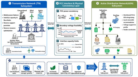
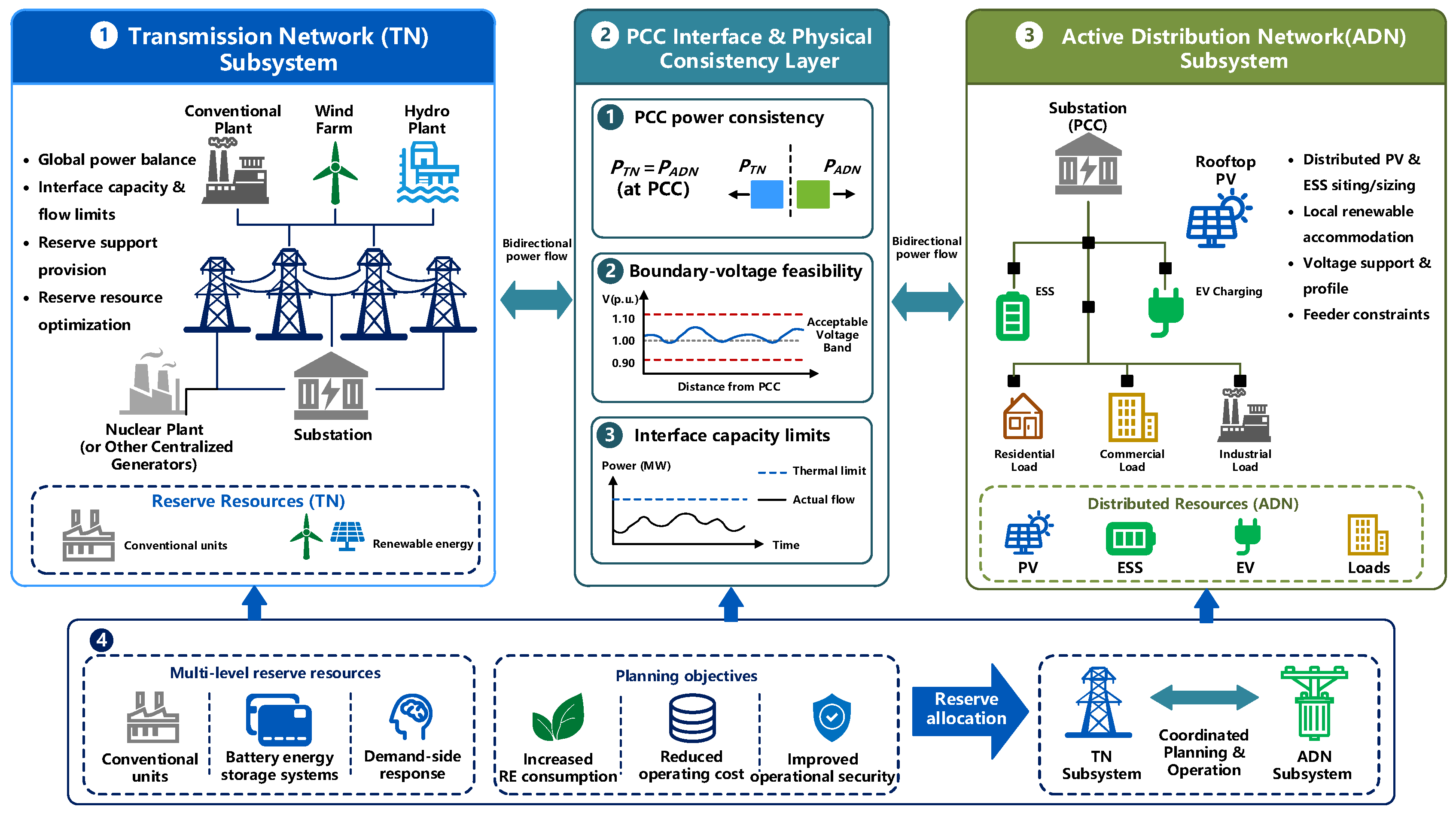
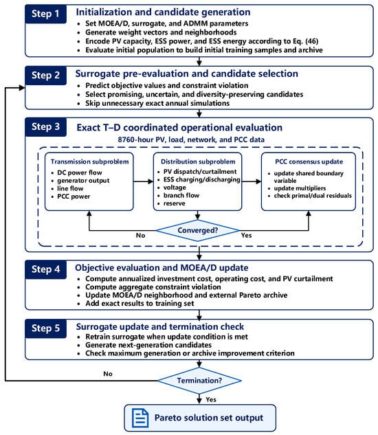
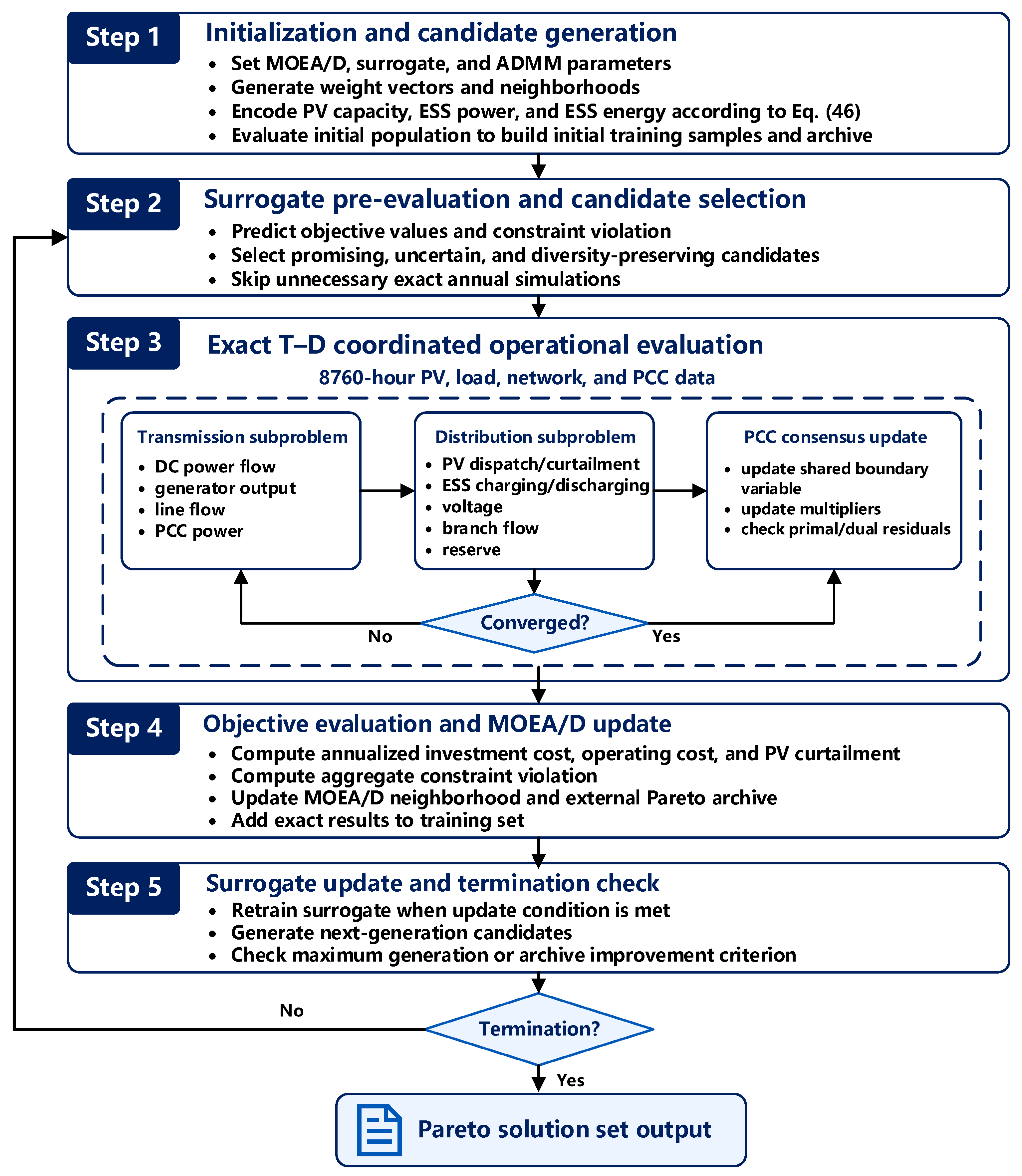
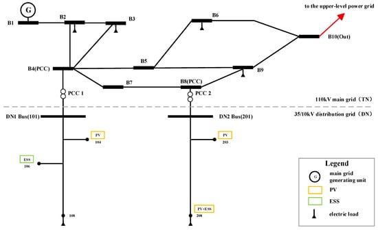
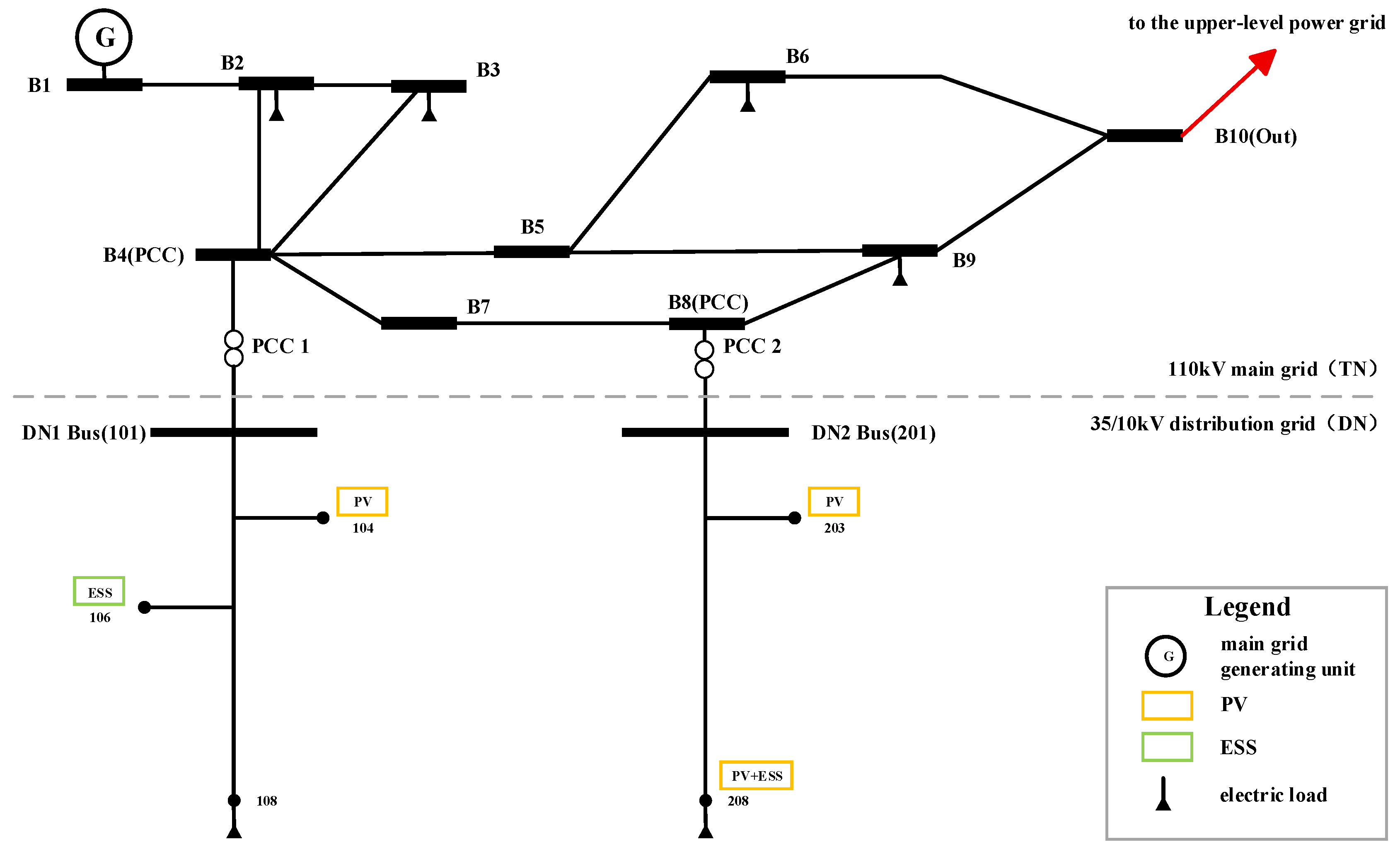
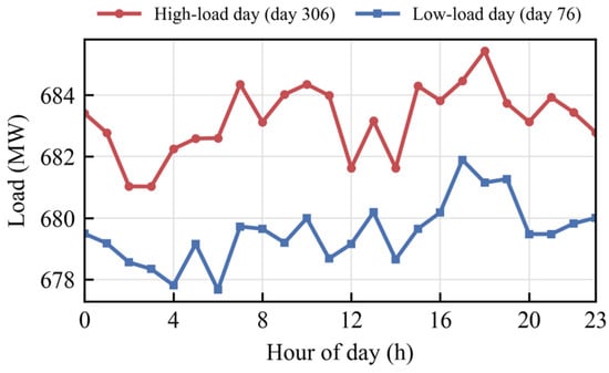
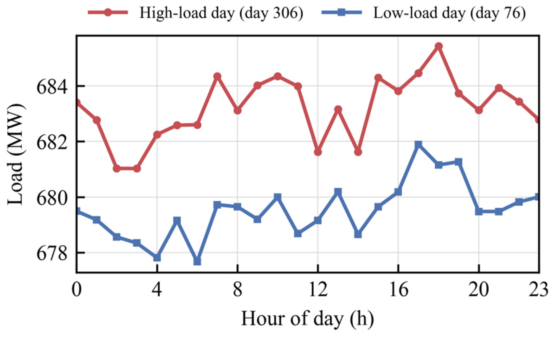
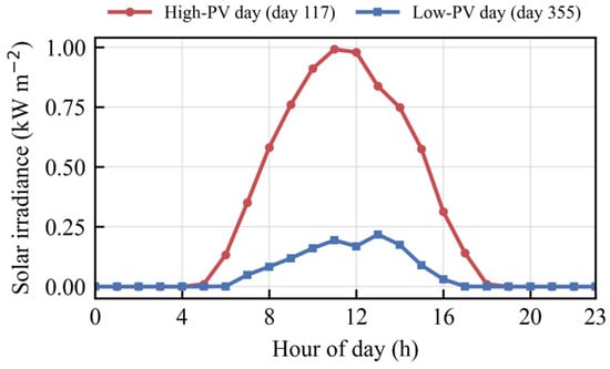
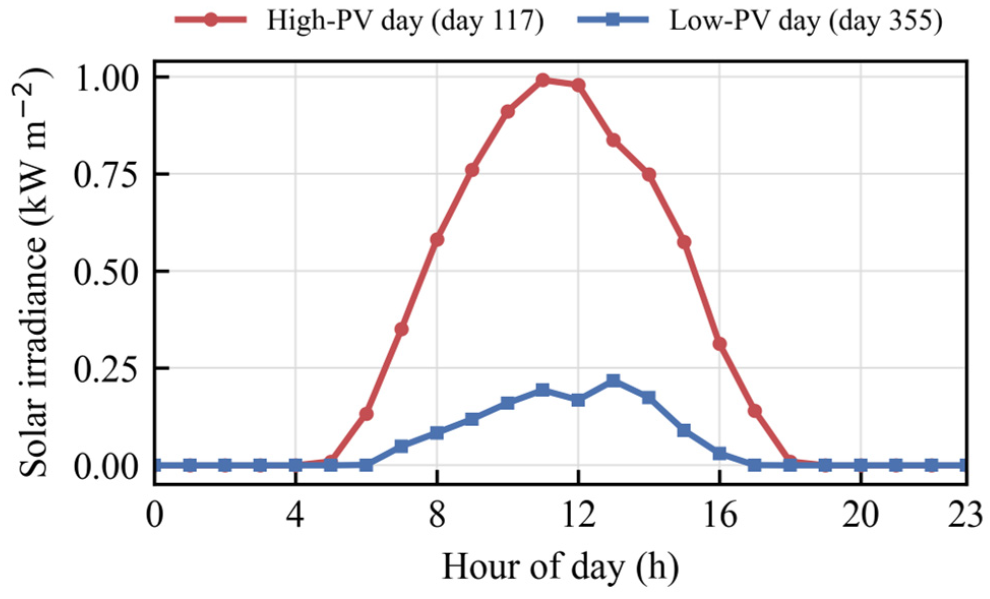
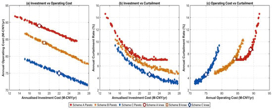
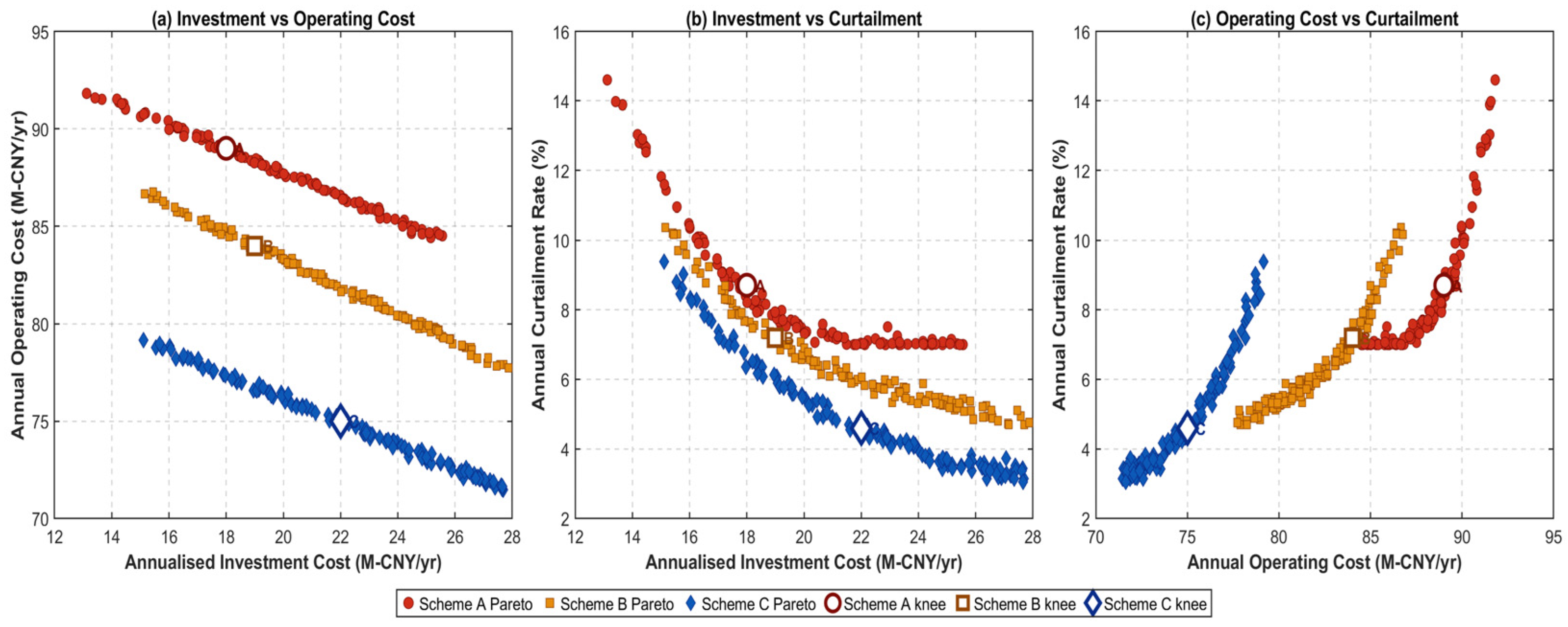
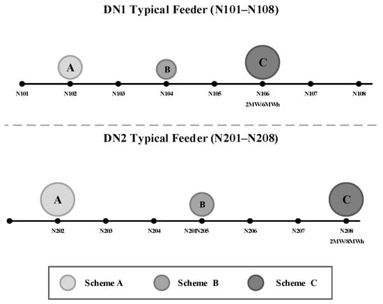
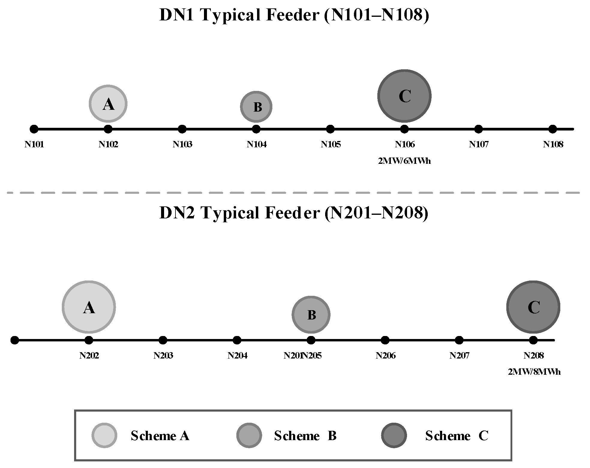
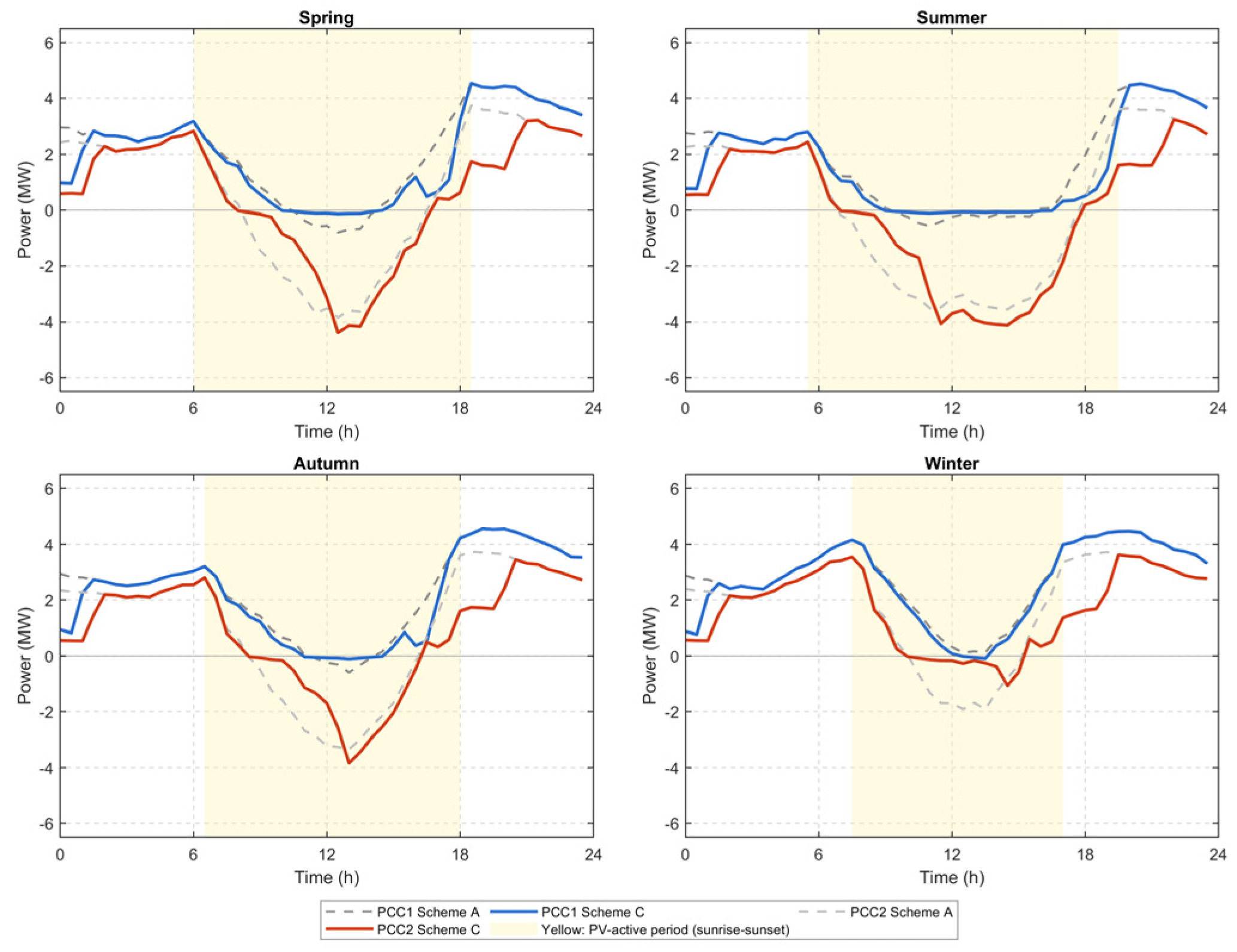
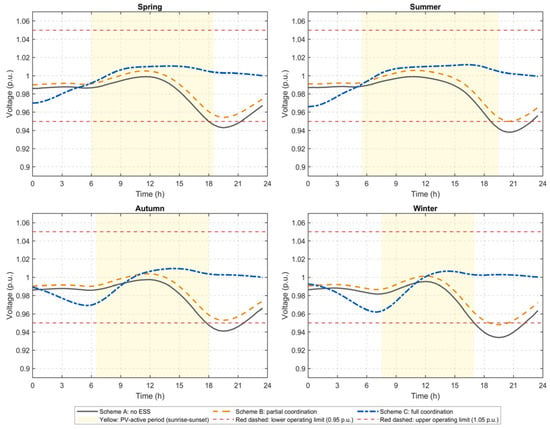
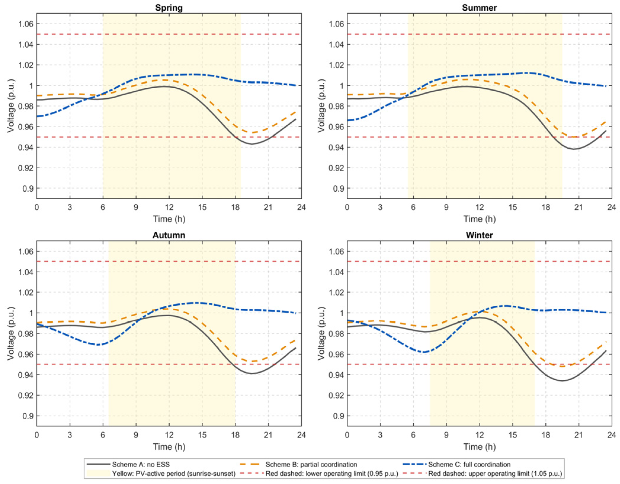
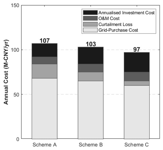
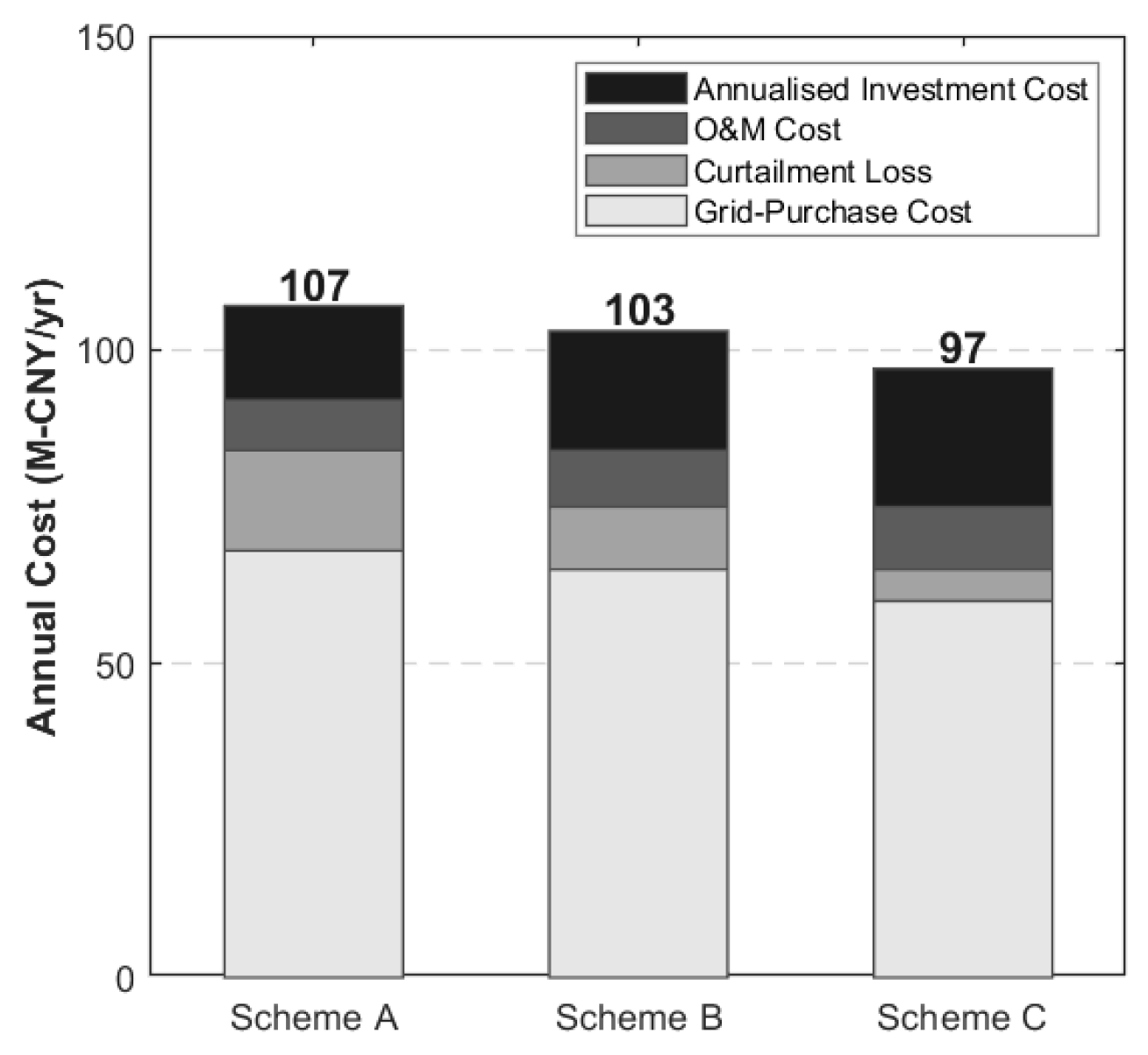

Disclaimer/Publisher’s Note: The statements, opinions and data contained in all publications are solely those of the individual author(s) and contributor(s) and not of MDPI and/or the editor(s). MDPI and/or the editor(s) disclaim responsibility for any injury to people or property resulting from any ideas, methods, instructions or products referred to in the content. |
© 2026 by the authors. Licensee MDPI, Basel, Switzerland. This article is an open access article distributed under the terms and conditions of the Creative Commons Attribution (CC BY) license.