A Finite-Domain Robust Framework for Effective Wave-Velocity Calibration and Microseismic Source Location in Meter-Scale Rock Specimens

Abstract

Locating fracture activity inside meter-scale rock specimens requires converting recorded wave arrivals into reliable source coordinates. In practice, this process is affected by uncertainty in wave velocity, abnormal arrival picks, incomplete sensor coverage, and the finite size of the specimen, which can lead to unstable or physically unreasonable locations. To address these issues, this study develops a finite-domain robust microseismic localization framework that integrates effective-velocity calibration, constrained source location, and robust treatment of abnormal observations within a unified workflow. The method was evaluated using controlled synthetic benchmarks covering different disturbance levels, propagation conditions, and timing errors. The results show that the proposed framework improves source-location accuracy and reduces large localization errors, with the clearest advantage under strongly disturbed arrival-time conditions and for events located near specimen boundaries. Additional sensitivity analyses demonstrate how propagation structure, sensor timing, and array configuration affect the estimated locations and effective velocity. The resulting workflow provides a reproducible and standardized approach for arrival-time-based microseismic localization in meter-scale rock specimens and offers a consistent basis for subsequent fracture interpretation and laboratory monitoring.

1. Introduction

During hydraulic fracturing, shock-wave stimulation, and mechanical loading of meter-scale rock specimens, the position and timing of internal fracture activity are needed to interpret the response to treatment. The rock is opaque: surface images show exposed traces, while post-test sectioning reveals the final fracture geometry. Microseismic and acoustic-emission (AE) monitoring provide spatial and temporal information by locating the sources of recorded elastic waves [1,2]. Experimental studies have complemented these observations with three-dimensional post-test fracture reconstruction [3], AE event locations in 2 m class specimens [4], and distributed fiber-optic measurements of fracture evolution [5]. The practical task is to convert these observations into source coordinates that can be interpreted within the known specimen geometry.

Arrival-time localization requires an appropriate propagation velocity and reliable onset picks. Waveform-based approaches also depend on travel-time prediction and array geometry [6]. In a meter-scale specimen, an incomplete surface array, abnormal picks, and uncertainty in the velocity used for processing can interact: a change in velocity shifts the fitted source position, and the optimizer may place a source outside the rock volume to reduce a timing residual. Probabilistic localization incorporates spatial information [7], while velocity-uncertainty analysis, calibration-shot methods, and simultaneous anisotropy estimation address the coupling between propagation and source position [8,9,10]. These studies establish the importance of evaluating velocity and location together.

The treatment of erroneous arrival picks provides a second route to improving location estimates. Ge compared absolute-value and least-squares objectives using calibrated AE/microseismic data [11]. Kurz examined three-dimensional localization with erroneous onset times in concrete specimens using propagation paths up to approximately 1 m [12]. Huber loss retains quadratic weighting for small residuals and reduces the influence of larger residuals through a linear penalty [13]. For meter-scale hydraulic-fracturing event clouds, adaptive connectivity and robust plane extraction can then organize noisy located events into dominant fracture geometries [14]. For a bounded rock specimen, robust residual treatment at the localization stage can be combined with the known physical source domain and an effective velocity selected from the event ensemble.

The methodological need is an integrated procedure for three coupled tasks: selecting a common localization velocity, locating events in the known rock volume, and assessing sensitivity to abnormal picks and array coverage. The contribution of such a procedure should be evaluated with controls that distinguish domain restriction from robust weighting. Source-position error, upper-tail error, and source-to-boundary behavior then reveal which part of the processing chain improves the spatial estimates. Independent propagation models and controlled timing offsets provide a separate assessment of the conditions governing application. Large-scale shock-wave–perforation experiments on 2 m shale blocks have also shown that different operation schemes can generate substantially different spatial fracture patterns and pressure responses [15], underscoring the value of a consistent source-location step before geometric interpretation.

This study presents FD-RML, which combines event-wise time centering, a finite source domain, Huber loss, and a multi-event velocity scan. A four-way synthetic comparison isolates the effects of the domain and loss function; model-mismatch and paired channel-delay tests assess propagation and timing sensitivity. The main numerical result is a reduction in mean and upper-tail location errors relative to finite-domain least squares, with the largest median-error reduction obtained under high disturbance. The method also provides sensor-deletion and truth-conditioned boundary diagnostics, supported by archived inputs, results, and code.

2. Materials and Methods

The workflow in Figure 1 takes P-wave picks and nominal sensor coordinates as inputs. First, event-wise centering removes the common unknown origin-time offset. Next, source coordinates are optimized within the specimen at each trial velocity, and the median event loss selects a shared effective velocity. Finally, location and sensitivity diagnostics characterize the estimates. Table 1 defines the notation and defaults. Equations (1)–(3) specify timing and centering, Equations (4)–(7) define the source and velocity searches, and Equations (8)–(12) define the diagnostic and comparison metrics. Diagnostics are evaluated after the arrival-time fit.

Figure 1. FD-RML workflow. The inner source search is repeated at each trial velocity; the outer multi-event objective selects the velocity. Error and stability are assessed separately from the spatial constraint.

Table 1. Main symbols and fixed numerical settings.

Symbol	Definition	Unit/Default
${\mathbf{x}}_{\mathrm{k}}$	Source coordinate of event k	m
${\mathbf{s}}_{\mathrm{i}}$	Nominal coordinate of sensor i	m
${\mathrm{t}}_{\mathrm{i}\mathrm{k}}^{\mathrm{o}\mathrm{b}\mathrm{s}}$	Observed arrival time	µs in implementation
${\mathrm{t}}_{0\mathrm{k}}$	Event-specific origin time	µs
${\mathrm{c}}_{\mathrm{i}}$	Dataset-fixed channel delay	µs
${\mathrm{v}}_{\mathrm{p}}$	Localization-effective constant velocity	m/s
$\mathsf{\Omega }$	Allowed source-coordinate set	[0, 2] × [0, 2] × [0, 1] m
$\mathsf{\delta }$	Huber transition	15 µs
$\mathrm{Q}\left({\mathrm{v}}_{\mathrm{p}}\right)$	Median of per-event mean losses	µs2
${\mathrm{S}}_{\mathrm{k}}$	Mean fixed-velocity deletion displacement	m
${\mathrm{d}}_0$	Near-boundary classification threshold	0.05 m

2.1. Arrival-Time Model and Effective Velocity

For event k and a valid sensor i, the matched-model observation equation is Equation (1). Times in Equation (1) are given in microseconds: the factor 10⁶ converts the distance/velocity travel time from seconds. The travel time uses Euclidean source-to-sensor distance, random pick error is denoted by ${\mathsf{\epsilon }}_{\mathrm{i}\mathrm{k}}$, and ${\mathrm{c}}_{\mathrm{i}}$ is fixed across events within a dataset. The inversion uses nominal sensor coordinates and does not estimate channel delays. Distinct forward models replace the travel-time term in Section 3.4 while leaving the inverse model unchanged.

$${\mathrm{t}}_{\mathrm{i}\mathrm{k}}^{\mathrm{o}\mathrm{b}\mathrm{s}}={\mathrm{t}}_{0\mathrm{k}}+{\displaystyle \frac{10^6\Vert {\mathbf{x}}_{\mathrm{k}}-{\mathbf{s}}_{\mathrm{i}}{\Vert }_2}{{\mathrm{v}}_{\mathrm{p}}}}+{\mathsf{\epsilon }}_{\mathrm{i}\mathrm{k}}+{\mathrm{c}}_{\mathrm{i}}$$

(1)

The fitted ${\mathrm{v}}_{\mathrm{p}}$ is the constant that best represents the centered arrival times for the adopted domain, array, loss, and event population. In a homogeneous isotropic control, it can be evaluated against the generating velocity. In an anisotropic or heterogeneous specimen, it summarizes the travel-time differences sampled by the source–sensor paths. It is therefore a localization-effective parameter rather than a unique material P-wave velocity. Sensor geometry, source distribution, channel availability, and systematic timing errors determine the paths and weights entering the fit [8,9,10]. This definition relates the parameter directly to its role in source-location inference [16].

2.2. Event-Wise Time Centering

Let ${\mathrm{N}}_{\mathrm{k}}$ be the number of valid channels, and define ${\mathrm{u}}_{\mathrm{i}\mathrm{k}}$ as the observed time minus the predicted travel time. Equation (2) removes a common event-specific temporal offset and is invariant to a constant added to all arrivals. It uses all valid channels without selecting a reference channel. Channel-dependent delays and propagation differences remain in the centered residuals and are examined in Section 4.6 and Section 4.7.

$${\mathrm{u}}_{\mathrm{i}\mathrm{k}}={\mathrm{t}}_{\mathrm{i}\mathrm{k}}^{\mathrm{o}\mathrm{b}\mathrm{s}}-{\displaystyle \frac{10^6\Vert {\mathbf{x}}_{\mathrm{k}}-{\mathbf{s}}_{\mathrm{i}}{\Vert }_2}{{\mathrm{v}}_{\mathrm{p}}}},\mathrm{ }\mathrm{ }\mathrm{ }\mathrm{ }{\mathrm{r}}_{\mathrm{i}\mathrm{k}}={\mathrm{u}}_{\mathrm{i}\mathrm{k}}-{\overline{\mathrm{u}}}_{\mathrm{k}},\mathrm{ }\mathrm{ }\mathrm{ }\mathrm{ }{\overline{\mathrm{u}}}_{\mathrm{k}}={\displaystyle \frac{1}{{\mathrm{N}}_{\mathrm{k}}}}{\sum }_{\mathrm{j}=1}^{{\mathrm{N}}_{\mathrm{k}}}{\mathrm{u}}_{\mathrm{j}\mathrm{k}}$$

(2)

For quadratic loss, Equation (3) gives the exact relationship between centered residuals and the complete set of pairwise differences. FD-RML applies the nonlinear Huber penalty directly to the mean-centered residuals in Equation (2); the quadratic equivalence does not extend to this objective. Mean centering introduces residual correlation and distributes the contribution of an abnormal pick across channels. The disturbance benchmark evaluates the resulting estimator as implemented.

$${\sum }_{\mathrm{i}=1}^{{\mathrm{N}}_{\mathrm{k}}}({\mathrm{u}}_{\mathrm{i}\mathrm{k}}-{\overline{\mathrm{u}}}_{\mathrm{k}}{)}^2={\displaystyle \frac{1}{{\mathrm{N}}_{\mathrm{k}}}}{\sum }_{\mathrm{i}<\mathrm{j}}({\mathrm{u}}_{\mathrm{i}\mathrm{k}}-{\mathrm{u}}_{\mathrm{j}\mathrm{k}}{)}^2$$

(3)

2.3. Finite Physical Source Domain

Equation (4) defines the physical source domain. For each trial velocity, Equation (5) minimizes the arrival-time loss over this closed box. The domain encodes the premise that the analyzed sources originate inside the specimen and prevents the optimizer from reducing residuals through external coordinates. Localization accuracy is evaluated separately against the known source positions in the synthetic tests.

$$\mathsf{\Omega }=\left\{(\mathrm{x},\mathrm{y},\mathrm{z}):0\le \mathrm{x}\le 2,\mathrm{ }0\le \mathrm{y}\le 2,\mathrm{ }0\le \mathrm{z}\le 1\right\}$$

(4)

$${\widehat{\mathbf{x}}}_{\mathrm{k}}\left({\mathrm{v}}_{\mathrm{p}}\right)={\mathrm{a}\mathrm{r}\mathrm{g}\mathrm{ }\mathrm{m}\mathrm{i}\mathrm{n}}_{\mathbf{x}\in \mathsf{\Omega }}{\mathrm{L}}_{\mathrm{k}}(\mathbf{x},{\mathrm{v}}_{\mathrm{p}})$$

(5)

2.4. Robust Loss and Velocity Search

The per-event loss is the mean over valid channels, giving events with different channel counts comparable scales. Equations (6) and (7) define Huber loss [13] and the outer velocity objective. Residuals and the transition δ are expressed in microseconds, giving loss in µs². The transition is fixed before evaluation; true source positions are used for performance assessment, not parameter selection.

$${\mathrm{L}}_{\mathrm{k}}^{\mathrm{H}}={\displaystyle \frac{1}{{\mathrm{N}}_{\mathrm{k}}}}{\sum }_{\mathrm{i}=1}^{{\mathrm{N}}_{\mathrm{k}}}{\mathsf{\rho }}_{\mathsf{\delta }}({\mathrm{r}}_{\mathrm{i}\mathrm{k}}),\mathrm{ }\mathrm{ }\mathrm{ }\mathrm{ }{\mathsf{\rho }}_{\mathsf{\delta }}(\mathrm{r})={\displaystyle \frac{{\mathrm{r}}^2}{2}}\mathrm{ }(\left|\mathrm{r}\right|\le \mathsf{\delta });\mathrm{ }\mathrm{ }\mathrm{ }\mathrm{ }\mathsf{\delta }(\left|\mathrm{r}\right|-{\displaystyle \frac{\mathsf{\delta }}{2}})\mathrm{ }(\left|\mathrm{r}\right|\ge \mathsf{\delta })$$

(6)

$$\mathrm{Q}({\mathrm{v}}_{\mathrm{p}})={\mathrm{m}\mathrm{e}\mathrm{d}\mathrm{i}\mathrm{a}\mathrm{n}}_{\mathrm{k}}\mathrm{ }{\mathrm{L}}_{\mathrm{k}}^{\mathrm{H}}({\widehat{\mathbf{x}}}_{\mathrm{k}}({\mathrm{v}}_{\mathrm{p}}),{\mathrm{v}}_{\mathrm{p}}),\mathrm{ }\mathrm{ }\mathrm{ }\mathrm{ }{\widehat{\mathrm{v}}}_{\mathrm{p}}={\mathrm{a}\mathrm{r}\mathrm{g}\mathrm{ }\mathrm{m}\mathrm{i}\mathrm{n}}_{{\mathrm{v}}_{\mathrm{p}}\in \mathrm{V}}\mathrm{Q}({\mathrm{v}}_{\mathrm{p}})$$

(7)

Velocities are scanned from 1400 to 3800 m/s in 100 m/s increments, followed by 25 m/s refinement within ±100 m/s of the best coarse velocity, clipped to the same range. At every trial velocity, each event is initialized from the two lowest-loss points on a 5 × 5 × 3 grid. The solution at the preceding evaluated velocity is an additional initial point. All starts are refined with bound-constrained L-BFGS-B [17], analytic gradients, at most 200 iterations, ftol = 10⁻¹², gtol = 10⁻⁶, and a maximum of 30 line-search steps. The solution with the lowest arrival-time objective among the attempted starts is retained.

A multistart check at the selected velocities uses six grid starts for each of the six high-disturbance datasets. The largest coordinate change for either finite-domain method is approximately 1.1 × 10⁻⁸ m, indicating consistent local refinement under this check. Optimization statuses, trial velocities, losses, and audit outputs are archived.

2.5. Location Accuracy and Diagnostic Metrics

Sensor-deletion stability measures sensitivity to channel removal at the selected velocity. Each valid channel is deleted once, and the source is relocated with velocity held fixed. Equation (8) gives the event-wise mean displacement across the deletions. This conditional sensitivity measure is reported alongside true-position error so that array sensitivity and absolute accuracy can be interpreted separately.

$${\mathrm{S}}_{\mathrm{k}}={\displaystyle \frac{1}{{\mathrm{N}}_{\mathrm{k}}}}{\sum }_{\mathrm{b}=1}^{{\mathrm{N}}_{\mathrm{k}}}\Vert {\widehat{\mathbf{x}}}_{\mathrm{k}}^{(-\mathrm{b})}-{\widehat{\mathbf{x}}}_{\mathrm{k}}{\Vert }_2$$

(8)

Event location error is the Euclidean distance to the known synthetic source. For dataset d, ${\mathrm{M}}_{\mathrm{d}}$ is the median event error and ${\mathrm{P}}_{\mathrm{d}}$ is the 90th percentile. Equation (9) averages these summaries over datasets to describe central and upper-tail performance. For homogeneous generating models, velocity error and the fraction of datasets within 5% additionally quantify recovery of the generating velocity. Section 3.4 defines the reference-velocity interpretation used for heterogeneous and anisotropic media.

$${\mathrm{e}}_{\mathrm{k}\mathrm{d}}=\Vert {\widehat{\mathbf{x}}}_{\mathrm{k}\mathrm{d}}-{\mathbf{x}}_{\mathrm{k}\mathrm{d}}^{\mathrm{t}\mathrm{r}\mathrm{u}\mathrm{e}}{\Vert }_2,\mathrm{ }\mathrm{ }\mathrm{ }\mathrm{ }{\mathrm{M}}_{\mathrm{d}}={\mathrm{m}\mathrm{e}\mathrm{d}\mathrm{i}\mathrm{a}\mathrm{n}}_{\mathrm{k}}\mathrm{ }{\mathrm{e}}_{\mathrm{k}\mathrm{d}},\mathrm{ }\mathrm{ }\mathrm{ }\mathrm{ }\overline{\mathrm{M}}={\displaystyle \frac{1}{\mathrm{D}}}{\sum }_{\mathrm{d}=1}^{\mathrm{D}}{\mathrm{M}}_{\mathrm{d}}$$

(9)

Geometric constraint satisfaction is the fraction of estimated coordinates in Ω. For both finite-domain methods, it is 100% determined by construction and document enforcement of the source-domain assumption; it is not an independent accuracy metric. All extended-domain estimates, including coordinates outside Ω, enter the localization-error calculations.

Boundary diagnostics distinguish the recovery of genuine near-face sources from assignment of interior sources to a near-face position. Equation (10) compares estimated and true nearest-face distances; negative $\mathsf{\Delta }{\mathrm{d}}_{\mathrm{k}}$ indicates a smaller estimated distance. The comparison uses distance to the nearest face, irrespective of face identity. Equation (11) reports recovery within the true near-boundary population and false attraction within the true interior population. Both classifications use a 0.05 m threshold. Summaries by true-distance bin relate these classifications to source location error.

$${\mathrm{d}}_{\mathrm{k}}^{\mathrm{t}\mathrm{r}\mathrm{u}\mathrm{e}}=\mathrm{d}({\mathbf{x}}_{\mathrm{k}}^{\mathrm{t}\mathrm{r}\mathrm{u}\mathrm{e}},\partial \mathsf{\Omega }),\mathrm{ }\mathrm{ }\mathrm{ }\mathrm{ }{\mathrm{d}}_{\mathrm{k}}^{\mathrm{e}\mathrm{s}\mathrm{t}}=\mathrm{d}({\widehat{\mathbf{x}}}_{\mathrm{k}},\partial \mathsf{\Omega }),\mathrm{ }\mathrm{ }\mathrm{ }\mathrm{ }\mathsf{\Delta }{\mathrm{d}}_{\mathrm{k}}={\mathrm{d}}_{\mathrm{k}}^{\mathrm{e}\mathrm{s}\mathrm{t}}-{\mathrm{d}}_{\mathrm{k}}^{\mathrm{t}\mathrm{r}\mathrm{u}\mathrm{e}}$$

(10)

$${\mathrm{R}}_{\mathrm{B}}=\mathrm{P}\mathrm{r}\left({\mathrm{d}}^{\mathrm{e}\mathrm{s}\mathrm{t}}<{\mathrm{d}}_0|{\mathrm{d}}^{\mathrm{t}\mathrm{r}\mathrm{u}\mathrm{e}}<{\mathrm{d}}_0\right),\mathrm{ }\mathrm{ }\mathrm{ }\mathrm{ }{\mathrm{F}}_{\mathrm{B}}=\mathrm{P}\mathrm{r}\left({\mathrm{d}}^{\mathrm{e}\mathrm{s}\mathrm{t}}<{\mathrm{d}}_0|{\mathrm{d}}^{\mathrm{t}\mathrm{r}\mathrm{u}\mathrm{e}}\ge {\mathrm{d}}_0\right)$$

(11)

Equation (12) defines the median paired improvement across datasets. This ensemble statistic is reported separately from a single-case difference and from the difference between ensemble means. Two-sided paired Wilcoxon tests [18] use the 24 dataset-level summaries. Location differences are rounded to 10⁻⁶ m and velocity-error differences to 10⁻⁸ percentage points before testing to control numerical ties. Holm correction [19] covers six comparisons based on three baselines and two endpoints. Descriptive 95% intervals for the median paired location improvement use 10,000 paired bootstrap resamples, stratified by scenario. The model and delay extensions use eight independent blocks each; comparisons across levels preserve that paired structure.

$$\mathsf{\Delta }{\mathrm{M}}_{\mathrm{p}\mathrm{a}\mathrm{i}\mathrm{r}\mathrm{e}\mathrm{d}}={\mathrm{m}\mathrm{e}\mathrm{d}\mathrm{i}\mathrm{a}\mathrm{n}}_{\mathrm{d}=1,...,24}({\mathrm{M}}_{\mathrm{d}}^{\mathrm{b}\mathrm{a}\mathrm{s}\mathrm{e}\mathrm{l}\mathrm{i}\mathrm{n}\mathrm{e}}-{\mathrm{M}}_{\mathrm{d}}^{\mathrm{F}\mathrm{D}-\mathrm{R}\mathrm{M}\mathrm{L}})$$

(12)

2.6. Computational Implementation and Data Provenance

All quantitative results use the synthetic realizations generated with master seed 20260928 and the implementation specified in Section 2.1, Section 2.2, Section 2.3, Section 2.4 and Section 2.5. This reanalysis retains the submitted disturbance design and specifies the optimizer in full. The current tables and figures use this consistent numerical dataset, while the submitted aggregate values are retained separately in the revision provenance record.

Calculations used Python 3.13.5, NumPy 2.3.5, and SciPy 1.17.0 [20,21]. The retained numerical record contains the fixed parameter settings, selected source and sensor coordinates, arrival-time inputs, channel masks, source estimates, velocity objectives, event errors, and numerical-check outputs supporting the reported tables and figures. Numerical checks cover noiseless recovery, origin-time invariance, analytic gradients, forward reciprocity, and propagation-model limiting cases. An independent 80-segment Fermat-path calculation agrees with the analytic gradient-model times within 0.000135% for 12 sampled source–receiver pairs.

3. Synthetic Benchmark Design

3.1. Specimen and Sensor Geometry

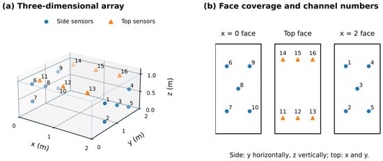
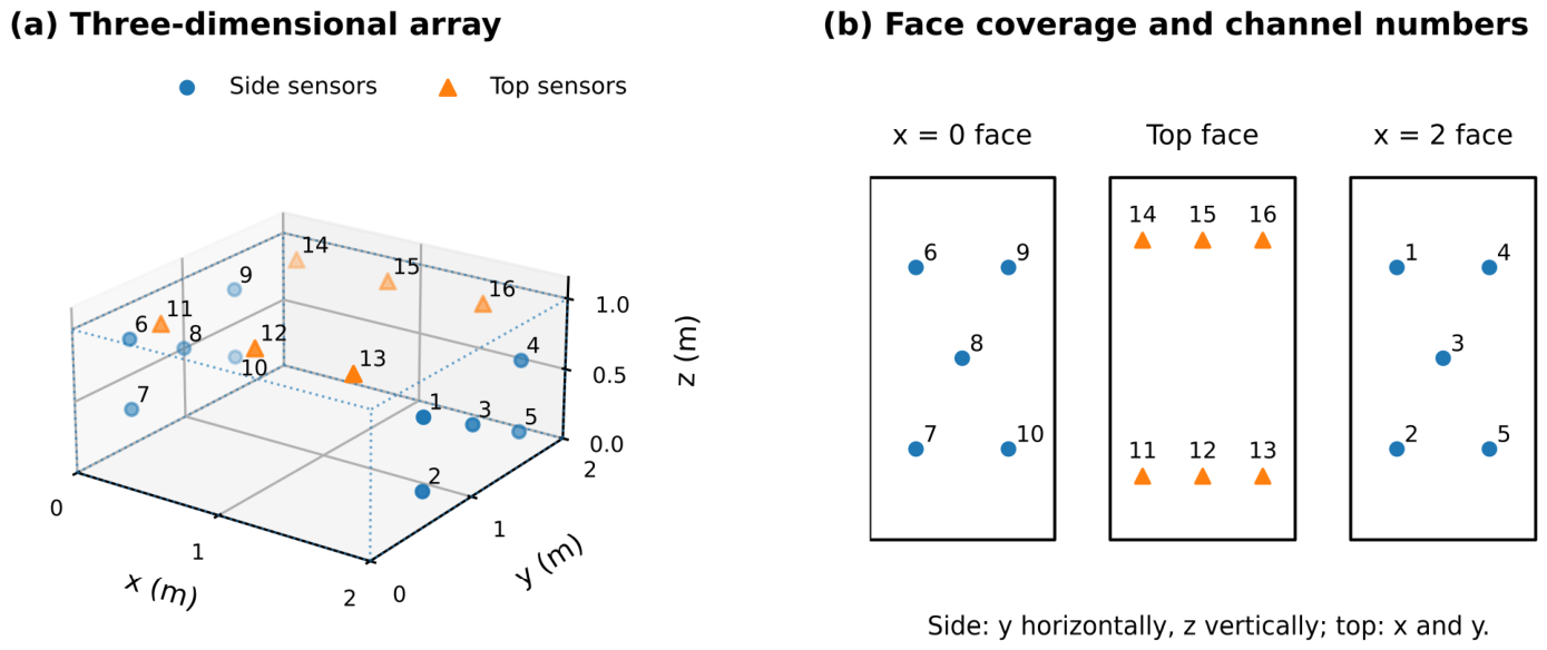
The synthetic specimen measures 2 m × 2 m × 1 m. Sixteen nominal sensors cover two opposite x faces and the top face, representing an incomplete laboratory surface array. Table 2 gives their coordinates and Figure 2 shows the geometry. The sensor-position perturbations specified in the matched-model benchmark enter the forward calculation, while the inverse calculation consistently uses the nominal coordinates.

Table 2. Nominal sensor coordinates used in all calculations.

Sensor	x (m)	y (m)	z (m)
1	2.00	0.50	0.75
2	2.00	0.50	0.25
3	2.00	1.00	0.50
4	2.00	1.50	0.75
5	2.00	1.50	0.25
6	0.00	0.50	0.75
7	0.00	0.50	0.25
8	0.00	1.00	0.50
9	0.00	1.50	0.75
10	0.00	1.50	0.25
11	0.35	0.35	1.00
12	1.00	0.35	1.00
13	1.65	0.35	1.00
14	0.35	1.65	1.00
15	1.00	1.65	1.00
16	1.65	1.65	1.00

Figure 2. Nominal geometry: (a) three-dimensional sensor arrangement; (b) separated projections of the two lateral faces and top face. Side-face drawings expand the vertical coordinate for legibility; Table 2 gives the numerical geometry.

3.2. Matched-Model Disturbance Benchmark

The matched-model benchmark isolates the effects of observation errors and domain restriction. Each of four disturbance scenarios contains six independent datasets of 18 events, giving 24 datasets and 432 distinct source realizations. The generating velocities within each scenario are 1800, 2200, 2600, 3000, 3400, and 2600 m/s. Interior coordinates are sampled uniformly from 0.1 m to the corresponding specimen dimension minus 0.1 m. A scenario-dependent number, obtained by rounding 18 times the near-face fraction in Table 3, is reassigned to a randomly selected face at a distance uniformly sampled between 0.015 and 0.080 m. The realized fraction within 0.05 m is calculated separately for boundary classification.

Table 3. Matched-model disturbance parameters.

Scenario	Pick σ (µs)	Outliers (%)	Outlier σ (µs)	Missing Channels	Delay σ (µs)	Sensor σ (mm)	Near-Face Generation (%)
Low	2.5	0	45	0	1	0	20
Moderate	7	4	70	1	3	2	25
High	13	10	110	3	7	5	30
Boundary-rich	9	6	85	2	5	3	55

Near-face generation uses distances of 0.015–0.080 m. The true fraction within the 0.05 m classification threshold is calculated from the generated coordinates. Sensor σ is the standard deviation applied to each Cartesian component.

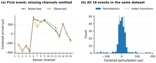
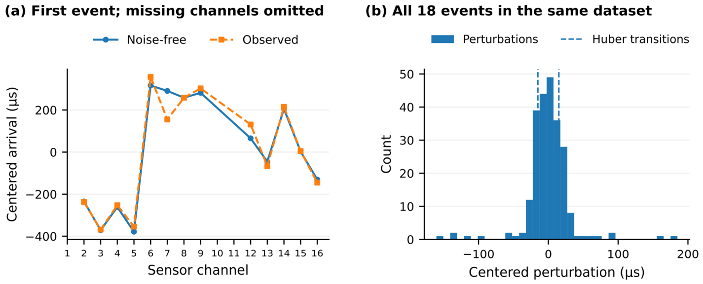
Arrival times are generated from the perturbed sensor coordinates with independent Gaussian pick noise, sparse additive Gaussian abnormal picks, dataset-fixed Gaussian channel delays, and a dataset-fixed missing-channel mask. Event origins are uniform from 0 to 4000 µs. Table 3 defines the controlled sensitivity settings, and the same observations are supplied to every compared method. Figure 3 illustrates centered perturbations in the third high-disturbance dataset, also used in Section 4.3. These amplitudes specify synthetic tests rather than measured distributions from a particular rock specimen.

Figure 3. Arrival-time disturbances in the representative high-disturbance dataset: (a) noise-free and observed centered arrivals for event 1 on valid channels; (b) centered perturbations for all 18 events. Missing channels are omitted from the observations.

3.3. Compared Methods

Table 4 defines a 2 × 2 comparison of source domain and loss. All methods share the centering, velocity grid, initialization rule, optimizer tolerances, and observations. Finite-domain L2 is the primary control for the incremental effect of Huber weighting. Extended-domain L2 and Huber provide complementary controls for the effect of source-domain restriction; their search region is the larger finite box specified in the table.

Table 4. Controlled comparisons; all methods share the velocity scan.

Method	Source-Search Domain	Loss
Extended-domain L2	−0.4 ≤ x, y ≤ 2.4; −0.3 ≤ z ≤ 1.3 m	Mean quadratic
Finite-domain L2	Physical specimen Ω	Mean quadratic
Extended-domain Huber	Same extended box	Mean Huber, δ = 15 µs
FD-RML	Physical specimen Ω	Mean Huber, δ = 15 µs

3.4. Independent Propagation-Model Mismatch

The independent propagation tests assess sensitivity to a forward model that differs from the inverse model, addressing the matched-model dependence associated with the inverse-crime concern [22]. Eight independent blocks are each evaluated under four forward models: a homogeneous control, elliptical anisotropy, a vertical velocity gradient, and a low-velocity layer. Source coordinates, origins, pick perturbations, channel delays, and masks are held fixed across the four models within each block. The 32 conditions contain 576 event realizations from eight independent source/noise blocks. Reference velocities are 1800, 2200, 2600, 3000, 3400, 2600, 2200, and 3000 m/s.

All model-mismatch conditions use nominal sensors, 7 µs Gaussian pick noise, a 4% abnormal-pick probability with 70 µs standard deviation, one missing channel, and 3 µs dataset-fixed delay standard deviation. The near-face generation fraction is 30%. Finite-domain L2 and FD-RML fit the same observations with the isotropic constant-velocity inverse model in Equation (1). The medium parameters define controlled synthetic propagation contrasts.

The anisotropic forward model uses an elliptical travel-time metric with directional velocities of ${\mathrm{v}}_{\mathrm{x}}=1.05 {\mathrm{v}}_0$, ${\mathrm{v}}_{\mathrm{y}}={\mathrm{v}}_0$, and ${\mathrm{v}}_{\mathrm{z}}=0.95 {\mathrm{v}}_0$, as defined in Equation (13). This model isolates the effect of directional travel speeds. Forward times T in Equations (13) and (14) are given in seconds and are multiplied by 10⁶ before observation perturbations are added.

$${\mathrm{T}}_{\mathrm{e}\mathrm{l}\mathrm{l}}=\sqrt{{\displaystyle \frac{(\mathrm{x}-{\mathrm{s}}_{\mathrm{x}}{)}^2}{{\mathrm{v}}_{\mathrm{x}}^2}}+{\displaystyle \frac{(\mathrm{y}-{\mathrm{s}}_{\mathrm{y}}{)}^2}{{\mathrm{v}}_{\mathrm{y}}^2}}+{\displaystyle \frac{(\mathrm{z}-{\mathrm{s}}_{\mathrm{z}}{)}^2}{{\mathrm{v}}_{\mathrm{z}}^2}}}$$

(13)

The gradient model uses a velocity profile $\mathrm{v}\left(\mathrm{z}\right)={\mathrm{v}}_0\left[1+0.20\left(\mathrm{z}-0.5\right)\right]$, ranging from 0.9 ${\mathrm{v}}_0$ to 1.1 ${\mathrm{v}}_0$ over the specimen height. With gradient $\mathrm{a}=0.20 {\mathrm{v}}_0$, endpoint velocities ${\mathrm{v}}_{\mathrm{s}}$ and ${\mathrm{v}}_{\mathrm{r}}$, and endpoint separation R, Equation (14) gives the unconstrained analytic ray time. Rays turning above z = 1 are replaced by the minimum path reaching the top face, traveling along that face, and returning to the receiver. The resulting curved or top-constrained path remains within the specimen. The numerical verification record includes an independent Fermat-path check.

$${\mathrm{T}}_{\mathrm{g}\mathrm{r}\mathrm{a}\mathrm{d}}={\displaystyle \frac{2}{\mathrm{a}}}\mathrm{a}\mathrm{s}\mathrm{i}\mathrm{n}\mathrm{h}\left({\displaystyle \frac{\mathrm{a}\mathrm{R}}{2\sqrt{{\mathrm{v}}_{\mathrm{s}}\mathrm{ }{\mathrm{v}}_{\mathrm{r}}}}}\right)$$

(14)

The low-velocity-zone model places a horizontal layer between z = 0.4 and 0.6 m at speed 0.75 ${\mathrm{v}}_0$, embedded in a medium of speed ${\mathrm{v}}_0$. Transmitted rays obey Snell’s law. Horizontal slowness is found by bisection from the horizontal offset, and segment times are summed over the layers. When both endpoints are in the slow layer, admissible critical head-wave paths along either interface are also evaluated. This idealized stratified medium isolates the effects of refraction and propagation-path changes.

For these mismatched media, ${\mathrm{v}}_0$ defines the reference speed scale. The evaluation reports source-position errors and signed deviations of fitted velocity from ${\mathrm{v}}_0$. These deviations describe the response of the effective scalar fit to directional or spatial velocity contrasts; they are not errors against a unique material velocity. Application conditions for these ray-based tests are discussed in Section 5.4.

3.5. Channel-Delay Sensitivity

The channel-delay experiment quantifies timing-induced bias using eight independent blocks with the homogeneous forward model and the pick-noise, outlier, and missing-channel settings of Section 3.4. In each block, a standard-normal channel-delay vector is multiplied by σc = 0, 1, 3, 5, 7, 10, or 15 µs while all other inputs remain fixed. The 56 conditions therefore comprise 1008 event realizations with eight independent source/noise blocks. Delays remain unestimated during inversion so their influence can be isolated. The absolute fitted-velocity shift from the same block’s zero-delay estimate is divided by ${\mathrm{v}}_0$ before averaging; this preserves the magnitude of shifts with opposite signs.

4. Results

4.1. Overall Matched-Model Performance

Table 5 shows the main location benefit over 24 matched-model datasets. With the same physical source domain, FD-RML reduces the mean dataset-median error from 0.0510 m for finite-domain L2 to 0.0403 m, a 20.9% reduction. The mean dataset P90 error decreases from 0.1034 to 0.0794 m, a 23.2% reduction, showing improvement in the upper tail as well as in the central error summary. Relative to extended-domain L2, the mean dataset-median reduction is 25.3%. Section 4.4 reports the corresponding paired inference.

Table 5. Matched-model performance across 24 datasets.

Method	Median v Error (%)	v Error ≤ 5% (%)	Mean M (m)	Mean P90 (m)	Constraint (%)
Extended-domain L2	1.14	95.8	0.0539	0.1268	86.8
Finite-domain L2	1.14	95.8	0.0510	0.1034	100.0
Extended-domain Huber	1.05	100.0	0.0426	0.0905	90.0
FD-RML	0.96	95.8	0.0403	0.0794	100.0

M is a within-dataset median; Mean M averages those 24 medians. Mean P90 averages within-dataset 90th percentiles. Constraint denotes geometric satisfaction and equals 100% automatically for finite-domain methods.

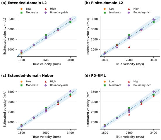
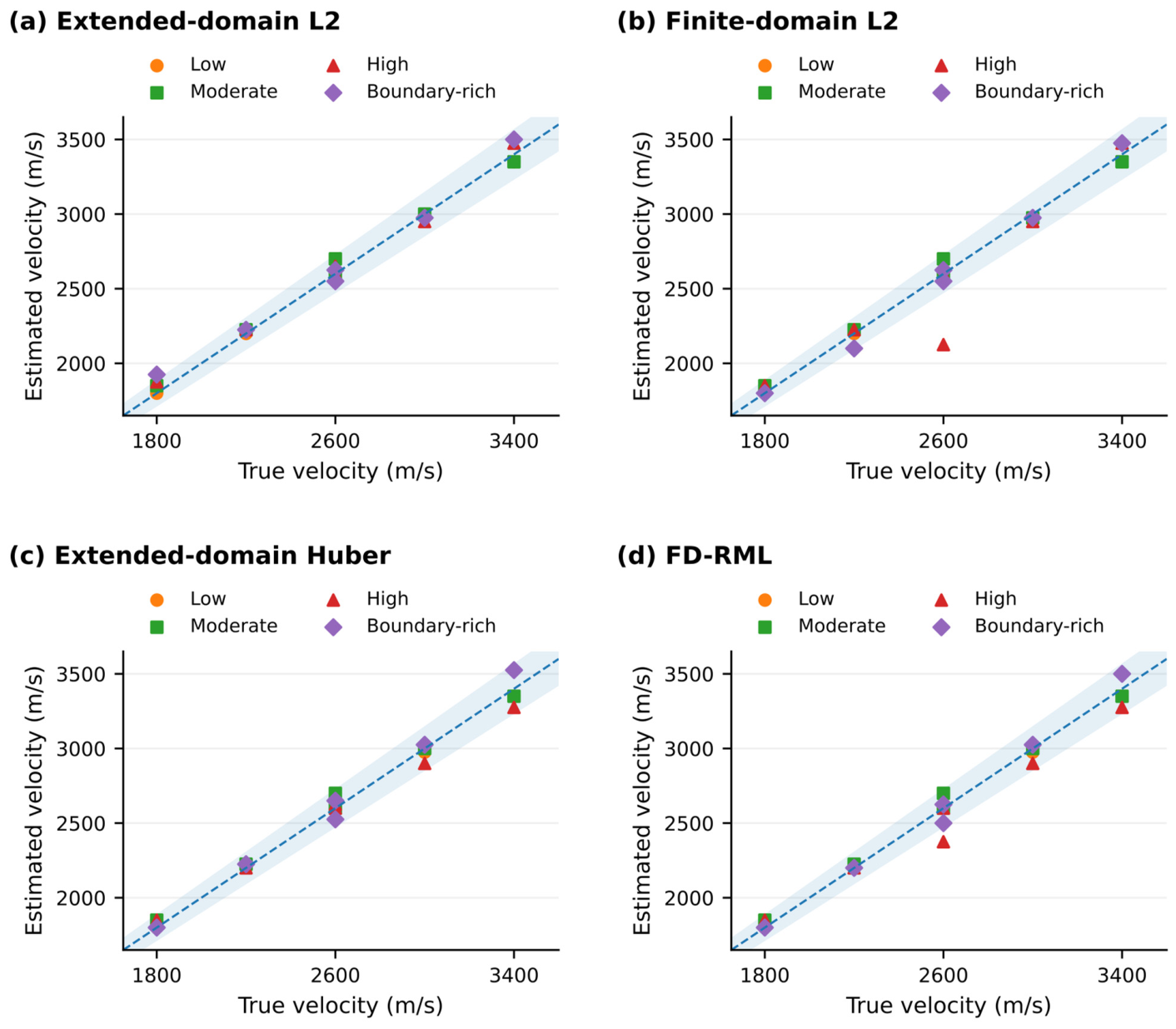
Figure 4 shows the selected velocities for all 24 datasets. FD-RML gives a median velocity error of 0.96%, compared with 1.14% for the L2 methods. FD-RML and both L2 controls recover velocity within 5% in 23 of 24 datasets; extended-domain Huber does so in 24 of 24. Velocity recovery and source-position error characterize different aspects of the coupled fit and are reported separately. The constraint column in Table 5 documents domain enforcement as defined in Section 2.5.

Figure 4. True versus selected velocity in the 24 homogeneous datasets: (a) extended-domain L2; (b) finite-domain L2; (c) extended-domain Huber; (d) FD-RML. The diagonal denotes exact recovery and the shaded band ±5%. All panels use identical limits.

4.2. Scenario-Specific Behavior

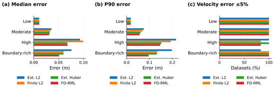
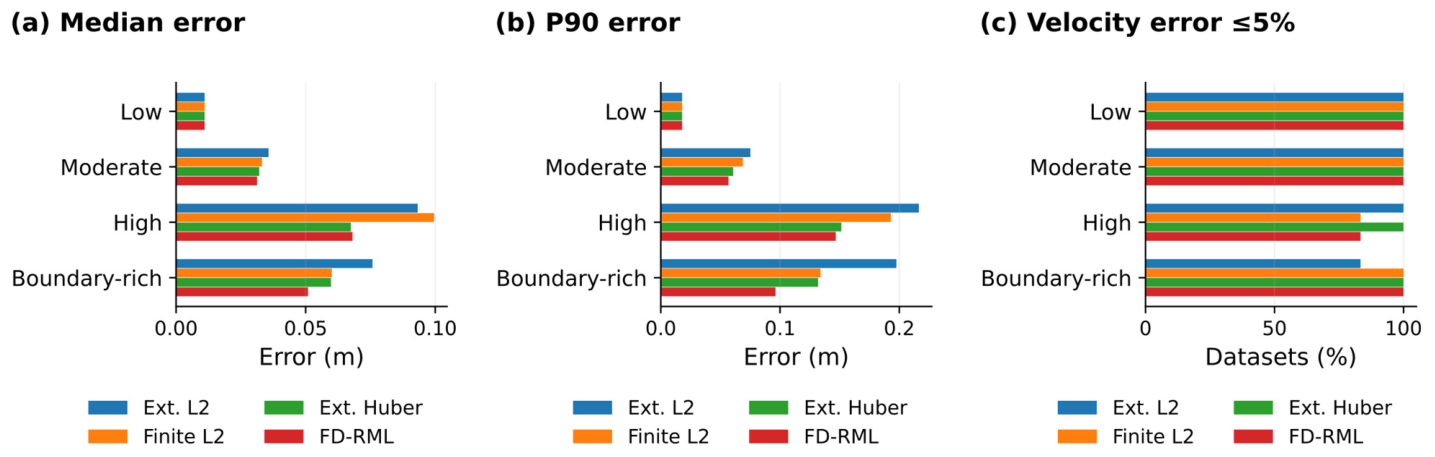
Table 6 and Figure 5 identify the disturbance conditions associated with the location gains. Under low disturbance, all four methods give a mean dataset-median error of 0.0110 m: sources are internal and the effective residuals lie in the quadratic regime. Under moderate disturbance, finite-domain L2 and FD-RML give 0.0332 and 0.0312 m. These controls connect the response of the robust objective to the level and structure of the arrival-time errors.

Table 6. Scenario-level summaries; six datasets per scenario.

Scenario	Method	Median v Error (%)	≤5% (%)	Mean M (m)	Mean P90 (m)
Low	Extended L2	0.42	100.0	0.0110	0.0179
Low	Finite L2	0.42	100.0	0.0110	0.0179
Low	Extended Huber	0.42	100.0	0.0110	0.0179
Low	FD-RML	0.42	100.0	0.0110	0.0179
Moderate	Extended L2	1.30	100.0	0.0357	0.0751
Moderate	Finite L2	1.30	100.0	0.0332	0.0688
Moderate	Extended Huber	1.30	100.0	0.0321	0.0607
Moderate	FD-RML	1.30	100.0	0.0312	0.0568
High	Extended L2	1.79	100.0	0.0932	0.2164
High	Finite L2	1.94	83.3	0.0996	0.1930
High	Extended Huber	1.87	100.0	0.0674	0.1515
High	FD-RML	3.06	83.3	0.0681	0.1467
Boundary-rich	Extended L2	1.53	83.3	0.0758	0.1976
Boundary-rich	Finite L2	1.44	100.0	0.0601	0.1339
Boundary-rich	Extended Huber	1.53	100.0	0.0598	0.1319
Boundary-rich	FD-RML	0.90	100.0	0.0509	0.0962

Figure 5. Scenario comparison of (a) mean dataset-median error, (b) mean dataset P90 error, and (c) the proportion of datasets within 5% velocity error. Each scenario contains six independent datasets.

The largest median-error reduction relative to finite-domain L2 occurs under high disturbance: 0.0996 to 0.0681 m, or 31.6%. Extended-domain Huber gives 0.0674 m in the same scenario, indicating that robust weighting accounts for much of this gain. In boundary-rich cases, finite-domain L2, extended-domain Huber, and FD-RML give 0.0601, 0.0598, and 0.0509 m, respectively. Combining the physical domain with robust weighting is therefore particularly useful for the near-face population in this benchmark. Figure 5 also shows the associated P90 errors.

4.3. Coupled Velocity and Location in a High-Disturbance Case

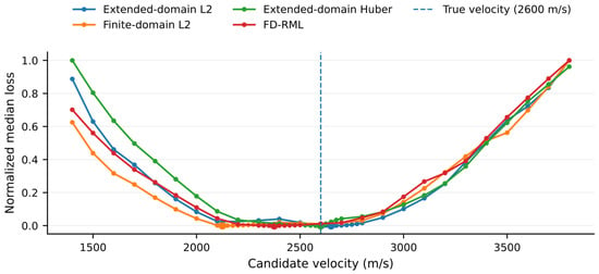
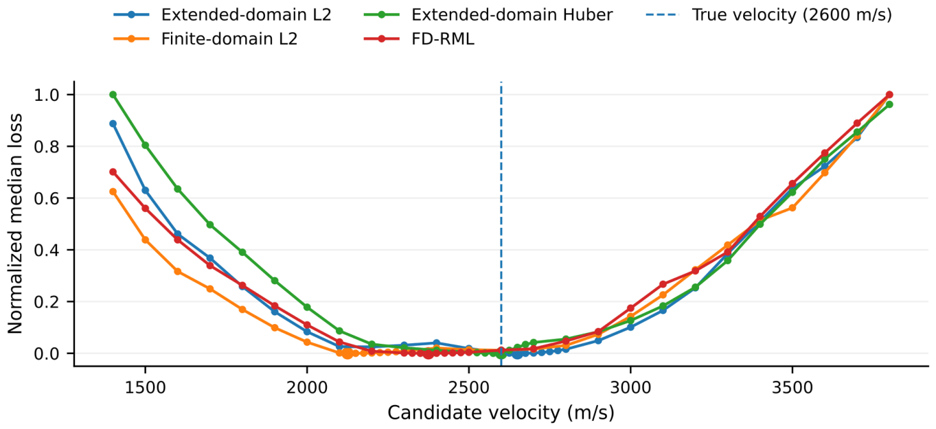
The third high-disturbance dataset (block 3) illustrates the coupling between the selected velocity and source position. Its generating velocity is 2600 m/s. In Figure 6, FD-RML selects 2375 m/s and finite-domain L2 selects 2125 m/s; the extended-domain Huber and L2 estimates are 2600 and 2650 m/s. The four objective profiles show how domain restriction and residual weighting alter the fitted velocity. Each curve is normalized separately to compare its shape.

Figure 6. Normalized velocity-profile objectives for the representative high-disturbance dataset. Markers indicate the selected minima, and the vertical reference denotes the generating velocity. Separate normalization enables comparison of profile shape; loss magnitudes are method-specific.

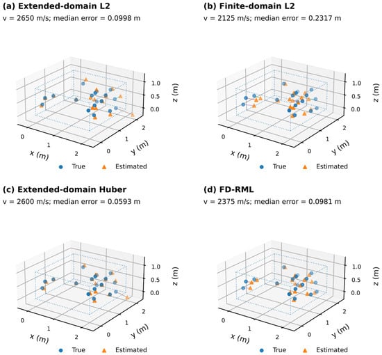
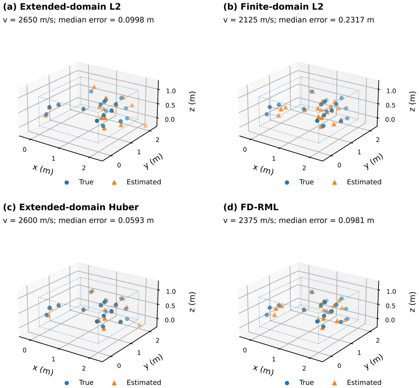
Figure 7 and Table 7 link these velocity estimates to source-position errors. Within the physical domain, Huber weighting reduces the case-specific median error from 0.2317 m for finite-domain L2 to 0.0981 m for FD-RML. The extended-domain L2 and Huber errors are 0.0998 and 0.0593 m, with 88.9% and 94.4% of their coordinates inside the specimen. This case separates three properties of the solution: the fitted velocity, distance to source truth, and domain satisfaction. Its 0.0017 m difference between extended-domain L2 and FD-RML is a single-dataset statistic; Section 4.4 evaluates the full ensemble.

Figure 7. True and estimated sources in the representative case: (a) extended-domain L2; (b) finite-domain L2; (c) extended-domain Huber; (d) FD-RML. Segments connect each estimate to its true source. Panels use identical extended display limits, with dotted lines marking the specimen.

Table 7. Representative dataset: true velocity 2600 m/s.

Method	Selected v (m/s)	v Error (%)	Median Error (m)	Constraint (%)
Extended-domain L2	2650	1.92	0.0998	88.9
Finite-domain L2	2125	18.27	0.2317	100.0
Extended-domain Huber	2600	0.00	0.0593	94.4
FD-RML	2375	8.65	0.0981	100.0

4.4. Paired Ensemble Comparisons

Table 8 evaluates all 24 paired datasets. The median paired location improvements are 0.0053 m relative to extended-domain L2, 0.0020 m relative to finite-domain L2, and approximately zero relative to extended-domain Huber. Equation (12) calculates these values from paired dataset medians. Table 7 reports a single-case comparison, while Table 5 reports ensemble means; the three summaries describe different features of the error distribution.

Table 8. Paired two-sided comparisons against FD-RML (24 dataset pairs).

Baseline	Median Paired Gain (m)	Bootstrap 95% Interval (m)	Location p (Raw/Holm)	Velocity p (Raw/Holm)
Extended-domain L2	0.0053	[0.0030, 0.0082]	0.0009/0.0052	0.5749/1.0000
Finite-domain L2	0.0020	[0.0000, 0.0050]	0.0108/0.0542	0.7794/1.0000
Extended-domain Huber	0.0000	[0.0000, 0.0024]	0.2026/0.8105	0.7505/1.0000

Positive gain denotes lower FD-RML error. Numerical endpoints near zero are printed as 0.0000 m. The bootstrap intervals are pointwise descriptive intervals; the Holm-adjusted p-values account for the six comparisons.

After Holm correction across the six comparisons, the location p-values are 0.0052 against extended-domain L2, 0.0542 against finite-domain L2, and 0.8105 against extended-domain Huber. At the adjusted 0.05 level, the first comparison is significant; the latter two and the velocity-error comparisons are not significant. The 20.9% mean and 23.2% P90 reductions relative to finite-domain L2 are descriptive effects in the tested ensemble. Together with the high-disturbance results, they locate the principal benefit in mean and upper-tail source error under the specified observation conditions.

4.5. Huber-Parameter and Sensor-Deletion Sensitivity

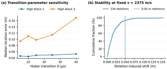
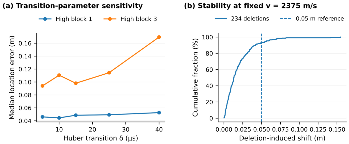
Figure 8a assesses how the Huber transition affects the coupled velocity–location fit in high-disturbance blocks 1 and 3. Across δ = 5–40 µs, median errors range from 0.0446 to 0.0527 m in block 1 and from 0.0940 to 0.1695 m in block 3. Changes in the selected velocity explain the non-monotonic response. This test provides context for interpreting a fixed robust-loss setting; all primary comparisons use the prespecified 15 µs transition.

Figure 8. Sensitivity diagnostics: (a) Huber-transition response in two high-disturbance blocks; (b) distribution of 234 one-channel-deletion shifts in block 3 at fixed selected velocity. The 0.05 m line provides a descriptive reference.

Figure 8b examines channel dependence by deleting each of 13 valid channels from each of 18 events in block 3, giving 234 fixed-velocity relocation trials. The median shift is 0.0131 m, the P90 shift is 0.0414 m, and the maximum is 0.1549 m; 93.16% of shifts lie within 0.05 m. The true-position median error for the same case is 0.0981 m. Reporting both quantities distinguishes sensitivity to array changes from the absolute error of the fitted location.

4.6. Location Sensitivity to Propagation Structure

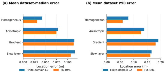
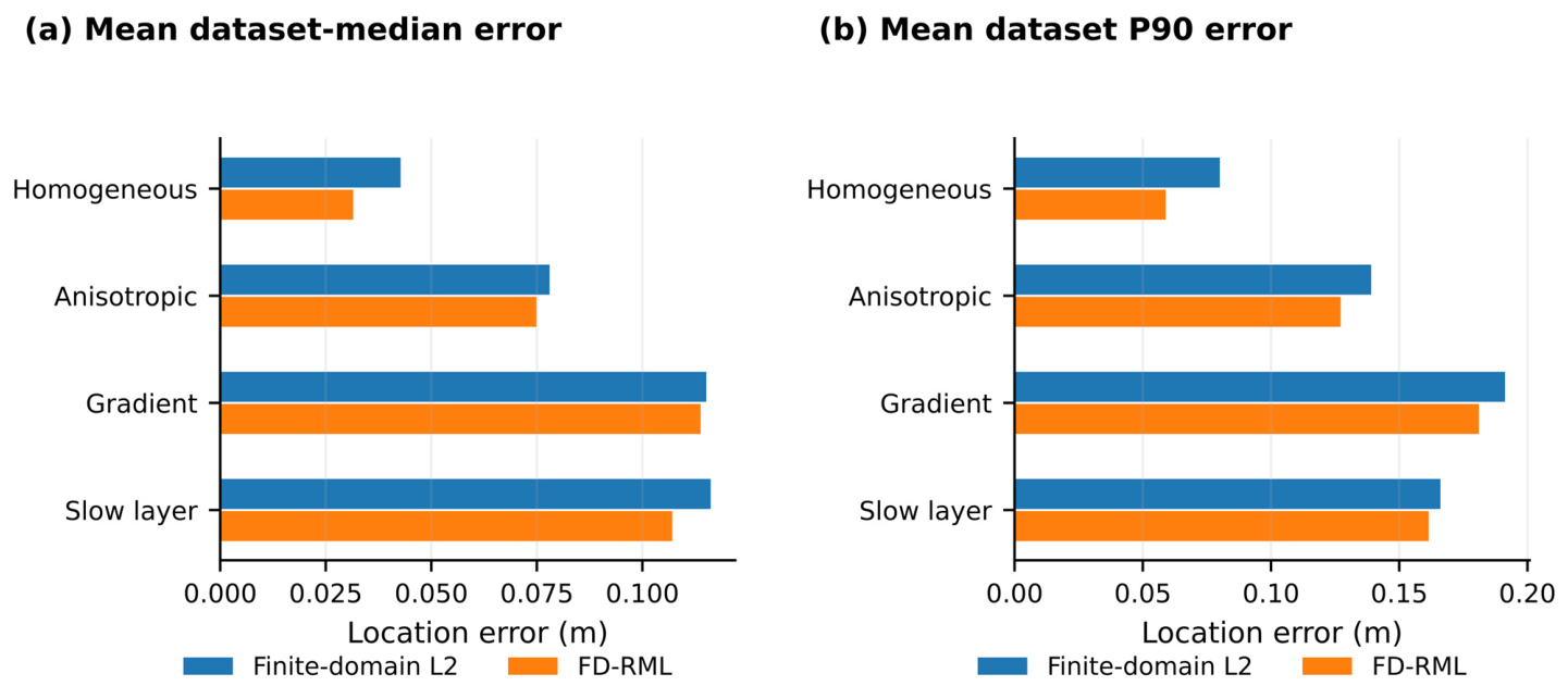
Table 9 and Figure 9 isolate propagation structure by applying the same inverse model to four forward media. FD-RML gives mean dataset-median errors of 0.0315 m in the homogeneous control, 0.0749 m under elliptical anisotropy, 0.1138 m under a vertical gradient, and 0.1071 m under a slow layer. Corresponding finite-domain L2 values are 0.0427, 0.0780, 0.1151, and 0.1162 m. The paired design separates propagation-induced error from changes in the source population or picking perturbations. It provides quantitative guidance on when refining the propagation model should take priority over further changes to the residual penalty.

Table 9. Independent forward-model conditions; eight matched blocks per model.

Forward Model	Inverse Method	Mean M (m)	Mean P90 (m)	Mean Signed v0 Deviation (%)
Homogeneous	Finite L2	0.0427	0.0800	+0.34
Homogeneous	FD-RML	0.0315	0.0589	+0.80
Elliptical anisotropy	Finite L2	0.0780	0.1390	+4.84
Elliptical anisotropy	FD-RML	0.0749	0.1272	+4.19
Vertical gradient	Finite L2	0.1151	0.1913	+1.32
Vertical gradient	FD-RML	0.1138	0.1811	+2.28
Slow layer	Finite L2	0.1162	0.1661	−3.67
Slow layer	FD-RML	0.1071	0.1614	−3.61

The reference v0 defines the synthetic speed scale; its deviation describes the fitted scalar response to the medium. Both inverse methods estimate a common scalar velocity and source positions with their original parameterization.

Figure 9. Propagation-structure sensitivity with an unchanged isotropic constant-velocity inverse model: (a) mean dataset-median location error; (b) mean dataset P90 error. Four forward media share the same eight paired source/noise blocks.

FD-RML’s mean signed fitted-velocity deviations from the reference scale are +4.19%, +2.28%, and −3.61% for anisotropy, gradient, and slow-layer conditions. The gradient case combines a +2.28% velocity-scale deviation with 0.1138 m location error. Thus, the interpretation of effective velocity benefits from direct source-position assessment: a scalar can summarize path-dependent travel times while the spatial estimates retain sensitivity to propagation structure.

4.7. Timing-Calibration Sensitivity

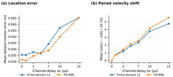
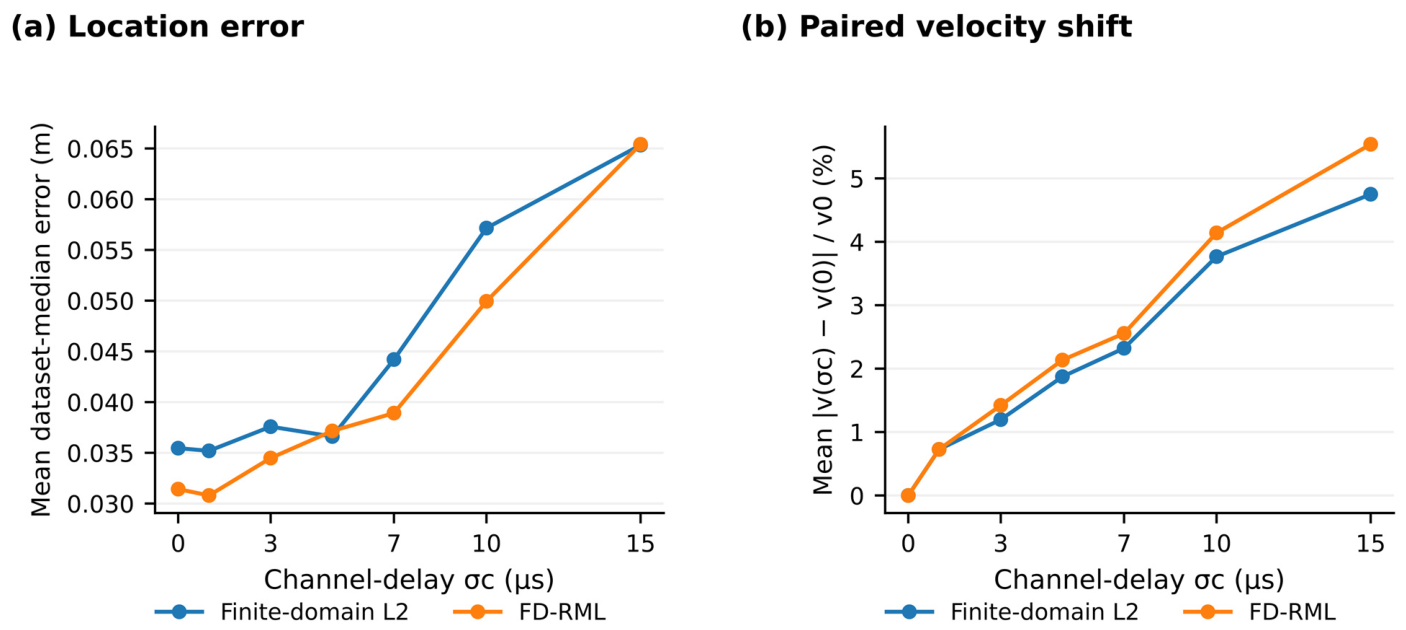
Table 10 and Figure 10 quantify the influence of channel-dependent timing offsets. Increasing σc from 0 to 15 µs changes FD-RML’s mean dataset-median error from 0.0314 to 0.0654 m. At 15 µs, the mean absolute velocity shift from the same block’s zero-delay fit is 5.54% of v0, and the mean signed deviation from v0 is −4.52%. Finite-domain L2 gives 0.0653 m location error at that level. The close endpoint errors identify a shared sensitivity to coherent channel timing, distinct from the sparse abnormal-pick treatment.

Table 10. Paired channel-delay sensitivity over eight independent blocks.

Delay σc (µs)	Finite L2 Mean M (m)	FD-RML Mean M (m)	Finite L2 |Δv|/v0 (%)	FD-RML |Δv|/v0 (%)
0	0.0355	0.0314	0.00	0.00
1	0.0352	0.0308	0.73	0.73
3	0.0376	0.0345	1.20	1.42
5	0.0366	0.0372	1.87	2.14
7	0.0442	0.0389	2.32	2.56
10	0.0572	0.0499	3.77	4.14
15	0.0653	0.0654	4.75	5.54

|Δv| refers to the absolute fitted-velocity change from the same block at zero delay, normalized by its v0 and then averaged. The seven delay levels share source/noise realizations.

Figure 10. Channel-delay sensitivity: (a) mean dataset-median location error; (b) mean absolute paired velocity shift from each block’s zero-delay estimate. All other inputs are fixed within each block.

The paired design holds the source population and other perturbations fixed, separating the additional timing effect from baseline error. Individual curves can be non-monotonic, where an imposed delay partly offsets another perturbation. For application, these results support treating channel timing calibration and robust event localization as complementary steps: the former addresses systematic offsets, while the latter controls the influence of abnormal residuals.

4.8. Boundary Behavior Conditioned on Source Truth

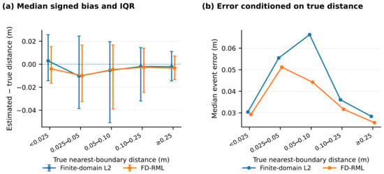
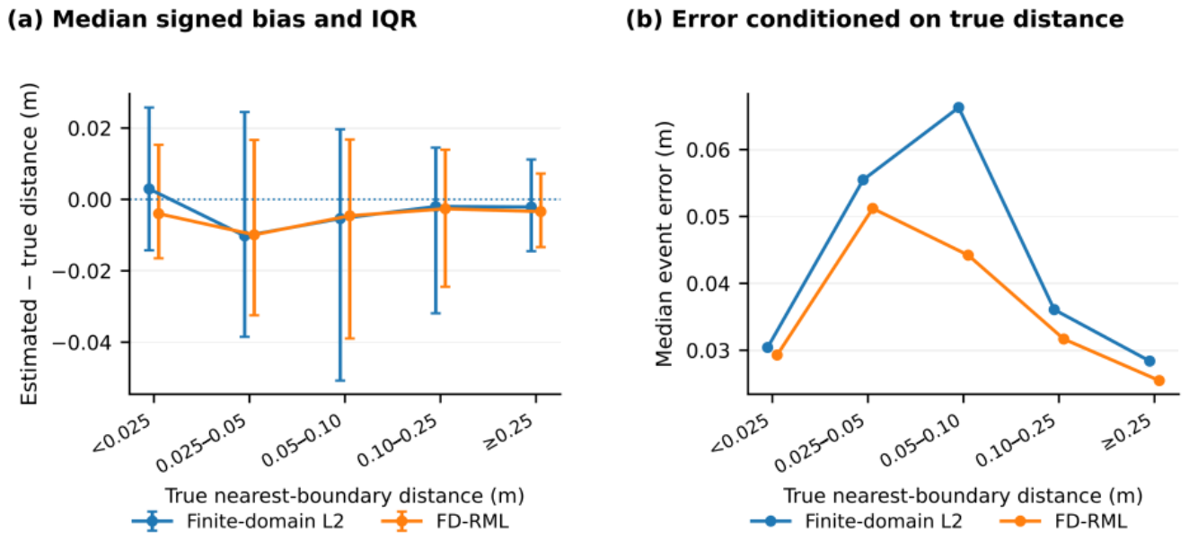
Figure 11 relates boundary behavior to the known source-to-boundary distance. The five true-distance bins contain 28, 52, 58, 161, and 133 events. For each bin, signed distance bias and its interquartile range describe the direction and spread of boundary displacement, while the median source-position error describes localization accuracy. These complementary summaries distinguish a geometric concentration near a face from its interpretation against source truth.

Figure 11. Boundary diagnostics for the finite-domain methods: (a) median estimated-minus-true nearest-face distance and interquartile range; (b) median location error in the same true-distance bins. Negative signed bias denotes a smaller estimated distance to the nearest face.

Of the 80 true sources within 0.05 m of a face, FD-RML places 65 in the same near-boundary class (81.25%). Among the 352 true interior sources, 33 are assigned to that class (9.38%). In the boundary-rich scenario, the corresponding fractions are 27/33 (81.82%) and 16/75 (21.33%). Reporting recovery and false attraction with separate denominators gives near-face event concentrations an explicit interpretation. These truth-conditioned diagnostics apply to the synthetic benchmark and to controlled tests with known source positions.

5. Discussion

5.1. Practical Contribution of the Integrated Workflow

FD-RML brings specimen geometry, effective-velocity selection, and robust residual weighting into one arrival-time procedure. Spatial prior information has a well-established role in probabilistic localization [7], and calibration-shot methods provide external constraints on the velocity model [9,23]. The present contribution is based on organizing these complementary ideas around a known meter-scale source volume and evaluating the resulting estimates with consistent inputs, controls, and diagnostics. This directly addresses the processing problem of coupled velocity and source coordinates in an incomplete surface array. Related studies provide complementary downstream measurements and interpretations through post-test fracture reconstruction, AE event clouds, distributed fiber-optic monitoring, robust event-cloud geometry extraction, and shock-wave–perforation physical modeling [3,4,5,14,15]. FD-RML addresses the upstream localization step that converts arrival times into source coordinates before those spatial analyses are performed.

The observed high-disturbance response is consistent with earlier AE/microseismic work on erroneous arrival picks. Ge’s calibrated absolute-value and least-squares comparison [11] and Kurz’s concrete localization study [12] link the location estimate to the treatment of problematic observations. Li et al. reported synthetic VFOM errors of approximately 10–20 m in a 400 m cubic array and evaluated six measured-position field blasts [24]. Those results provide cross-scale methodological context; the present quantitative effect sizes come from same-data comparisons in a 2 m specimen, with geometry, phase selection, and error summaries held consistent. The recent adaptive event-cloud reconstruction workflow [14] is complementary: it operates on located events to recover fracture geometry, whereas FD-RML focuses on the preceding arrival-time-to-coordinate step. The strongest result here is the reduction in source-position error when abnormal picks are prominent. Relative to finite-domain L2, the high-disturbance mean dataset-median error decreases by 31.6%; across the full benchmark, mean and P90 errors decrease by 20.9% and 23.2%. The low-disturbance control produces the same 0.0110 m error for all methods, linking the gain to disturbance treatment. Boundary-rich cases additionally show the contribution of combining robust weighting with the physical domain. These effects, interpreted with the paired statistics in Section 4.4, support the method’s use for arrival-time datasets containing both ordinary and abnormal picks.

5.2. Effective Velocity and Calibration Priorities

The effective velocity connects the travel-time model to the geometry actually sampled by the array and events. Calibration-shot studies [9,23], velocity-uncertainty analysis [8], and simultaneous anisotropy estimation [10] provide complementary ways to constrain that relationship. In FD-RML, the fitted scalar depends on the source–sensor paths and weights entering Equation (7). The propagation and timing tests demonstrate this dependence directly. Rechecking calibration when array geometry, loading state, or the event population changes maintains a consistent physical interpretation of the fitted value.

The two sensitivity experiments identify distinct calibration priorities. The propagation tests use ray bending or refraction to quantify the effect of a travel-time law different from that used for inversion. The channel-delay tests hold propagation fixed and quantify sensor-dependent timing bias. Together, they distinguish observation errors suited to robust residual treatment from systematic effects addressed through propagation characterization and timing calibration. This distinction provides a practical basis for choosing the next improvement to a monitoring workflow.

5.3. Interpreting Location Diagnostics

The diagnostic set assigns a separate meaning to each spatial result. Constraint satisfaction documents compliance with the specimen domain. Sensor deletion measures dependence on individual channels at fixed velocity. Truth-conditioned boundary analysis separates recovery of genuine near-face sources from false assignment of interior sources. Using these outputs together makes the interpretation of a source cloud more explicit than relying on its apparent shape or near-boundary occupancy.

The statistical design follows the unit of replication. The primary benchmark has 24 independent datasets and six per scenario; each extension has eight independent blocks reused across its model or delay levels. Paired tests and scenario-stratified bootstrap intervals preserve that structure. The reported mean and tail-error gains describe the tested ensembles, while Section 4.4 provides the corrected inference for the main comparisons.

5.4. Application Conditions

The intended setting is a meter-scale specimen with known dimensions and sensor coordinates, identifiable P-wave arrivals, and an event population for which a common effective velocity is a useful processing approximation. The present evidence is numerical: no known-location physical-source experiment is included. Quantitative application to rock measurements requires controlled-source calibration and independent validation positions spanning the region of interest; surface-source coverage should be distinguished from interior-source coverage.

The forward tests represent directional speed, curved rays, and a stratified low-velocity zone. Pick noise, abnormal picks, and missing channels represent observation-level perturbations. Attenuation, scattering, mode conversion, waveform distortion, and the detection process are not explicitly modeled. Their evaluation requires waveform-based or physical-source tests. The fixed inputs and documented numerical procedure provide a defined reference for those extensions and for comparing laboratory calibration results on a common processing basis.

6. Conclusions

• FD-RML integrates effective-velocity selection and source localization within a known specimen volume. Event-wise centering and robust residual weighting provide a consistent arrival-time processing procedure, complemented by location and sensitivity diagnostics.
• In 24 synthetic datasets containing 432 events, FD-RML reduces the mean dataset-median error from 0.0510 to 0.0403 m relative to finite-domain L2. The corresponding mean P90 error decreases by 23.2%, linking the benefit to both central and upper-tail location errors.
• The largest median-error reduction relative to finite-domain L2 is 31.6% under high disturbance. In boundary-rich cases, FD-RML gives a mean dataset-median error of 0.0509 m. These descriptive results identify abnormal-pick treatment and near-face localization as the principal strengths within the tested benchmark.
• Independent propagation-model and paired timing tests quantify how effective velocity and source position respond to medium structure and channel delays. Together with sensor-deletion and boundary diagnostics, they provide a basis for interpreting estimates and prioritizing calibration.
• The study establishes a reproducible, numerically tested workflow for effective-velocity calibration and microseismic source location in meter-scale specimens. Fixed parameter settings, retained numerical outputs, and diagnostic results provide a common reference for controlled-source testing and subsequent laboratory use.

References

- Maxwell, S.C. Microseismic Imaging of Hydraulic Fracturing: Improved Engineering of Unconventional Shale Reservoirs; Society of Exploration Geophysicists: Tulsa, OK, USA, 2014; Volume 17. [Google Scholar] [CrossRef] [Scilit]
- Grechka, V.; Heigl, W.M. Microseismic Monitoring; Society of Exploration Geophysicists: Tulsa, OK, USA, 2017; Volume 22. [Google Scholar] [CrossRef] [Scilit]
- Jiang, C.; Niu, B.; Yin, G.; Zhang, D.; Yu, T.; Wang, P. CT-based 3D reconstruction of the geometry and propagation of hydraulic fracturing in shale. J. Pet. Sci. Eng. 2019, 179, 899–911. [Google Scholar] [CrossRef] [Scilit]
- Dong, J.; Zhang, J.; Xie, B.; Wang, L.; Wang, X.; Guo, X.; Teng, J.; Li, J. Hydraulic Fracture Propagation in Three Meter-Scale Reconstituted Tight Conglomerate Specimens Under Different Formulation Conditions. Processes 2026, 14, 2573. [Google Scholar] [CrossRef] [Scilit]
- Zhang, Q.; Hou, B.; Wu, A.; Zhang, B.; Chen, G.; Yang, G.; Sun, T. Feature identification in multi-cluster true triaxial hydraulic fracturing using integrated fiber optic and acoustic emission monitoring. Measurement 2026, 258, 119363. [Google Scholar] [CrossRef] [Scilit]
- Li, L.; Tan, J.; Schwarz, B.; Staněk, F.; Poiata, N.; Shi, P.; Diekmann, L.; Eisner, L.; Gajewski, D. Recent advances and challenges of waveform-based seismic location methods at multiple scales. Rev. Geophys. 2020, 58, e2019RG000667. [Google Scholar] [CrossRef] [Scilit]
- Lomax, A.; Virieux, J.; Volant, P.; Berge-Thierry, C. Probabilistic earthquake location in 3D and layered models. In Advances in Seismic Event Location; Thurber, C.H., Rabinowitz, N., Eds.; Springer: Dordrecht, The Netherlands, 2000; pp. 101–134. [Google Scholar] [CrossRef] [Scilit]
- Gesret, A.; Desassis, N.; Noble, M.; Romary, T.; Maisons, C. Propagation of the velocity model uncertainties to the seismic event location. Geophys. J. Int. 2015, 200, 52–66. [Google Scholar] [CrossRef] [Scilit]
- Jiang, H.Y.; Chen, Z.B.; Zeng, X.X.; Lv, H.; Liu, X. Velocity calibration for microseismic event location using surface data. Pet. Sci. 2016, 13, 225–236. [Google Scholar] [CrossRef] [Scilit]
- Grechka, V.; Singh, P.; Das, I. Estimation of effective anisotropy simultaneously with locations of microseismic events. Geophysics 2011, 76, WC143–WC155. [Google Scholar] [CrossRef] [Scilit]
- Ge, M. Comparison of least squares and absolute value methods in AE/MS source location: A case study. Int. J. Rock Mech. Min. Sci. 1997, 34, 93.e1–93.e7. [Google Scholar] [CrossRef]
- Kurz, J.H. New approaches for automatic threedimensional source localization of acoustic emissions—Applications to concrete specimens. Ultrasonics 2015, 63, 155–162. [Google Scholar] [CrossRef] [Scilit] [PubMed]
- Huber, P.J. Robust estimation of a location parameter. Ann. Math. Stat. 1964, 35, 73–101. [Google Scholar] [CrossRef] [Scilit]
- Wang, X.; Deng, X.; Zhang, J.; Wang, L.; Wang, W.; Cong, R. Adaptive Connectivity and Robust Plane Extraction from Microseismic Event Clouds: A Systematic Benchmark and Conditional Case Study. Processes 2026, 14, 2961. [Google Scholar] [CrossRef] [Scilit]
- Xie, B.; Zhang, J.; Chen, X.; Zhang, Y.; Li, J.; Li, Q.; Teng, J.; Guo, J. Large Scale Physical Modeling of Shale Fracture Propagation Under Different Controllable Shock Wave and Perforation Operation Schemes. Processes 2026, 14, 3041. [Google Scholar] [CrossRef] [Scilit]
- Tarantola, A. Inverse Problem Theory and Methods for Model Parameter Estimation; Other Titles in Applied Mathematics; Society for Industrial and Applied Mathematics: Philadelphia, PA, USA, 2005. [Google Scholar] [CrossRef] [Scilit]
- Byrd, R.H.; Lu, P.; Nocedal, J.; Zhu, C. A limited memory algorithm for bound constrained optimization. SIAM J. Sci. Comput. 1995, 16, 1190–1208. [Google Scholar] [CrossRef] [Scilit]
- Wilcoxon, F. Individual comparisons by ranking methods. Biom. Bull. 1945, 1, 80–83. [Google Scholar] [CrossRef] [Scilit]
- Holm, S. A simple sequentially rejective multiple test procedure. Scand. J. Stat. 1979, 6, 65–70. [Google Scholar]
- Harris, C.R.; Millman, K.J.; van der Walt, S.J.; Gommers, R.; Virtanen, P.; Cournapeau, D.; Wieser, E.; Taylor, J.; Berg, S.; Smith, N.J.; et al. Array programming with NumPy. Nature 2020, 585, 357–362. [Google Scholar] [CrossRef] [Scilit] [PubMed]
- Virtanen, P.; Gommers, R.; Oliphant, T.E.; Haberland, M.; Reddy, T.; Cournapeau, D.; Burovski, E.; Peterson, P.; Weckesser, W.; Bright, J.; et al. SciPy 1.0: Fundamental algorithms for scientific computing in Python. Nat. Methods 2020, 17, 261–272. [Google Scholar] [CrossRef] [Scilit] [PubMed]
- Wirgin, A. The inverse crime. arXiv 2004, arXiv:math-ph/0401050. [Google Scholar] [CrossRef] [Scilit]
- Bardainne, T.; Gaucher, E. Constrained tomography of realistic velocity models in microseismic monitoring using calibration shots. Geophys. Prospect. 2010, 58, 739–753. [Google Scholar] [CrossRef] [Scilit]
- Li, X.B.; Wang, Z.W.; Dong, L.J. Locating single-point sources from arrival times containing large picking errors (LPEs): The virtual field optimization method (VFOM). Sci. Rep. 2016, 6, 19205. [Google Scholar] [CrossRef] [Scilit] [PubMed]
Disclaimer/Publisher’s Note: The statements, opinions and data contained in all publications are solely those of the individual author(s) and contributor(s) and not of MDPI and/or the editor(s). MDPI and/or the editor(s) disclaim responsibility for any injury to people or property resulting from any ideas, methods, instructions or products referred to in the content. |
© 2026 by the authors. Licensee MDPI, Basel, Switzerland. This article is an open access article distributed under the terms and conditions of the Creative Commons Attribution (CC BY) license.