Digital Objective Lens: A Lightweight Neural Network for Super-Resolution of SEM Images

Abstract

Scanning electron microscopy (SEM) is a crucial and frequently employed tool for material characterization. However, owing to the hardware limitations of SEM, researchers often face a trade-off when observing materials: they must either use the fast scanning mode to acquire real-time images with poor details or wait 20 to 160 s for the slow scanning mode to obtain a high-resolution (HR) image with rich details. This significantly reduces observation efficiency and prevents process-level observations. In this study, we propose a wavelet-based lightweight super-resolution (SR) network (WLSR), which serves as a “digital objective lens”: by performing rapid SR on fast-scan SEM images, 2× or 4× digital magnification of the field of view with slow-scan image quality can be obtained while large-scale observation of the sample is conducted. A channel–spatial attention block and a wavelet-based upscaling module are introduced into the network structure, and a novel loss function combining a wavelet distillation loss and a perceptual loss is proposed for network training. WLSR was trained and evaluated on paired fast-/slow-scan SEM images of AgCl@Ag specimens, in which all LR inputs are genuine fast-scan images that are jointly denoised and super-resolved. Compared with existing lightweight SR networks, WLSR generates SEM SR images with richer details, superior subjective visual quality, and competitive objective evaluation metrics at an exceptionally fast inference speed of 3.7 ms per image on an NVIDIA GV100 GPU, indicating the feasibility of real-time deployment during live SEM observation. Through WLSR, the quality of fast-scan SEM images is significantly improved, which can enhance the efficiency and accuracy of sample observation.

1. Introduction

Scanning electron microscopy (SEM) is the most versatile and commonly used observation method for observing the structure and morphology of materials [1,2,3]. It has the advantages of high resolution (HR), large depth of field, simple specimen preparation and dynamic observation. By launching a finely focused beam of electrons at the specimen and capturing the secondary and back-scattered electrons produced by their interaction with the specimen, SEM is able to provide images containing information about morphology, structure, composition and crystallography of the specimen [4,5,6].

In SEM, there are two modes available for researchers: the fast scanning mode, which captures low resolution (LR) images in real-time, and the slow scanning mode, which requires 20–160 s to obtain a single HR, detail-rich image. Researchers typically use the fast scanning mode to obtain LR images for quickly surveying the material surface and identifying regions of interest, and then switch to the slow scanning mode to acquire clear, HR images of these regions. However, this observation workflow is a necessary compromise due to the limitations of the SEM hardware [7]. First, the LR images obtained in real-time lack sufficient detail, making it easy to overlook regions of interest during observation. Second, the prolonged image acquisition time in the slow scanning mode significantly reduces observational efficiency. Ideally, HR, high-quality SEM images should be obtained in real-time for optimal observation [8,9,10].

Nowadays, super-resolution (SR) methods based on deep learning are widely applied to various SR tasks [11,12,13], such as thermal image SR [14], microscopic image SR [15], video SR [16], and so on [17,18,19,20]. The SR of SEM images has also been studied for a long time [21,22,23]. De Haan et al. [24] achieve resolution enhancement in SEM images using a generative adversarial network (GAN); by using this technique, higher resolution SEM images can be taken faster [25,26]. Wang et al. [27] designed a deep residual attention network based on residual learning and the attention mechanism; they created a microscopic butterfly wing dataset and trained an SR model that can super-resolve SEM images of butterfly wings. Fan et al. [28] proposed a two-stage SR method based on RCAN and GAN to super-resolve SEM images of AgCl@Ag nanoparticles; HR SEM images can be acquired without sample damage by using this method. Furat et al. [29] deployed SRGANs to super-resolve SEM images of cracked cathode materials. This method enables representative quantification of fine features, which benefits crack detection within aged cathode particles. Wang et al. [30] employed a diffusion model-based SR network, significantly enhancing the quality of fast scanning mode SEM images.

Before presenting our method, we clarify the term super-resolution in the context of this work. For SEM operators, resolution is a physical parameter corresponding to the diameter of the electron probe, which defines the spatial limit of the information that an image can carry. Digital image processing modifies experimentally obtained information rather than acquiring new information, and therefore cannot improve the physical resolution of the microscope itself. Throughout this paper, SR refers to a computational restoration task: the network learns the statistical mapping from fast-scan LR images to the slow-scan HR images of the same field of view, such that the digitally magnified output reproduces the sharpness and detail appearance of the corresponding slow-scan image. The recovered details are jointly determined by the information content of the acquired fast-scan image and the image prior learned from the training data, and never exceed the physical resolution limit of the microscope; that is, WLSR restores image information that is attenuated or masked during fast scanning instead of creating information beyond the electron–specimen interaction.

However, these SEM SR models are deep and large, which is not suitable for real-time SEM SR [31,32,33]. Here, we propose WLSR, a wavelet-based lightweight SR network to solve the above problem. We compare WLSR to a “digital objective lens”; by using it to perform rapid super-resolution on fast-scan SEM images, digital 2× or 4× magnification of the field of view can be obtained with an inference speed that supports real-time display during live observation, while conducting a large-scale observation of the sample. For WLSR’s network structure, we use a channel–spatial attention mechanism in the feature extraction module to make the network pay more attention to more important channels and spatial locations, and we use a wavelet-based upscale module to better reconstruct the information in different frequency bands. For the loss function, we propose a loss function which contains the wavelet distillation loss and the perceptual loss instead of simply using the mean absolute error (MAE) loss; the wavelet distillation loss is achieved through knowledge distillation and the Wavelet Upscale. The wavelet distillation loss can encourage WLSR to focus on the information in different frequency bands and the perceptual loss can encourage WLSR to focus on the subjective visual quality of SR images. The MAE loss always leads SR networks to the over-smooth problem; using our loss function instead can encourage SR networks to generate images with more high-frequency details. Compared to other existing lightweight SR networks, WLSR provides the best subjective visual quality, with a Learned Perceptual Image Patch Similarity (LPIPS) [34] score of 0.2055 and a Fréchet Inception Distance (FID) [35] score of 8.90 in the X2 SR task. WLSR also provides competitive objective evaluation metrics, with a Peak Signal to Noise Ratio (PSNR) score of 28.36 and a Structure Similarity Index Measure (SSIM) score of 0.7141 with the inference time of 3.7 ms/image in the X2 SR task, which indicates that fast acquisition and HR image appearance can be achieved at the same time. The contributions of this paper can be succinctly summarized as follows:

• We propose a novel loss function which contains the wavelet distillation loss and the perceptual loss; the loss function can encourage the network to generate SR images with better details.
• We present a lightweight SR network WLSR for fast SEM image enhancement by introducing the channel–spatial attention mechanism and a wavelet-based upscale module; its millisecond-level inference speed supports real-time deployment during SEM observation. Compared to other lightweight SR networks, WLSR can generate SR images with the most detail information, the best subjective visual quality and competitive objective evaluation metrics.

2. Materials and Methods

2.1. WLSR Network Structure

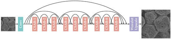
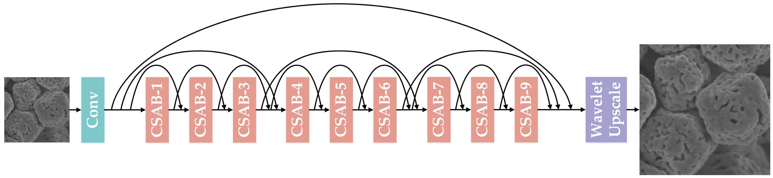
As shown in Figure 1, WLSR, the lightweight SR network we propose, is mainly composed of three parts: the shallow feature extraction module, the deep feature extraction module and the Wavelet Upscale. Throughout this work, all LR images are fast-scan images and all HR references are slow-scan images acquired from the same field of view (Section 2.3); WLSR is therefore trained to map the noisy fast-scan appearance to the clean slow-scan appearance. Given $I_{LR}$ as the LR image input, WLSR uses one convolutional layer to extract the shallow feature $I_{SF}$ from the LR image input (1):

$$I_{SF}=F_{SF}\left(I_{LR}\right)$$

(1)

Figure 1. The network structure of WLSR.

$F_{SF}(·)$ denotes the shallow feature extraction module, and its output, the shallow feature maps $I_{SF}$, will go through the deep feature extraction module for deep feature extraction (2):

$$I_{DF}=F_{DF}\left(I_{SF}\right)$$

(2)

$F_{DF}(·)$ denotes the deep feature extraction module which contains several channel–spatial attention blocks (CSABs). In order to simplify the training of the network and accelerate the fitting of the network, we add a short skip connection for each CSAB, a middle skip connection for every three CSABs and a long skip connection for the overall nine CSABs. Through the deep feature extraction module, WLSR provides a large receptive field size, and the deep feature maps can be obtained. Finally, those deep feature maps $I_{DF}$ are upscaled by the Wavelet Upscale to produce the final SR image (3):

$$I_{SR}=F_{WU}\left(I_{DF}\right)=F_{WLSR}\left(I_{LR}\right)$$

(3)

$F_{WU}(·)$ and $F_{WLSR}(·)$ denote the Wavelet Upscale and WLSR, respectively.

2.1.1. Channel–Spatial Attention Block

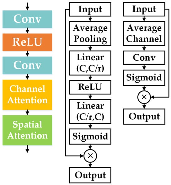
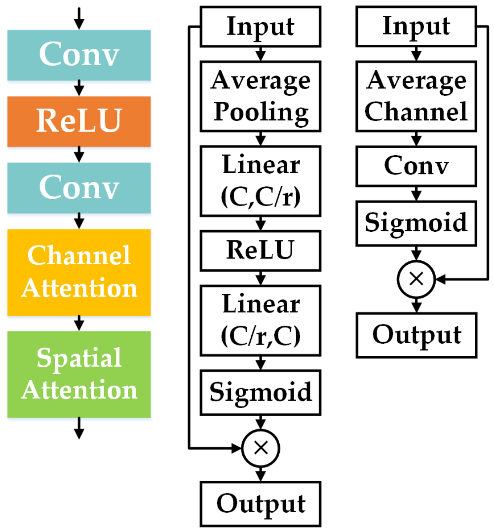
We use multiple CSABs in order to extract deep feature maps from the LR image. As shown in Figure 2, the CSAB consists of two convolutional layers, the ReLU function, the channel attention module and the spatial attention module.

Figure 2. (Left) CSAB, (Middle) channel attention module, (Right) spatial attention module.

Previous SR networks treat channel-wise feature maps equally, which wastes abundant computing resources on feature channels with little or no information; this is inefficient and inflexible. The channel attention module exploits the channel inter-dependencies of the feature maps, which allows WLSR to focus more on informative feature channels. The input feature maps $I_{input}\in R^{H\times W\times C}$ go through an average pooling layer $P_{avg}^c(·)$; by calculating the average value $V_{avg}^c$ of each feature channel, the amount of information of different feature channels can be preliminarily judged (4):

$$V_{avg}^c=P_{avg}^c\left(I_{input}\right)={\displaystyle \frac{1}{H\times W}}{\displaystyle \sum _{i=1}^H}{\displaystyle \sum _{j=1}^W}{I}_{input}(i,j)\in R^{1\times 1\times C}$$

(4)

Then the average value $V_{avg}^c$ of each feature channel goes through a simple gating mechanism that includes a channel downscaling layer $W_D$ with ratio r, the ReLU function, a channel upscaling layer $W_U$ with ratio r and the sigmoid function. By using this simple gating mechanism, the channel inter-dependencies of the feature maps can be calculated and the channel scaling factor $s_c$ can be obtained (5):

$$s_c=Sigmoid\left(W_{U}ReLU\left(W_D{V}_{avg}^c\right)\right)\in R^{1\times 1\times C}$$

(5)

Finally, the channel-wise adaptively rescaled feature maps $I_c$ are obtained (6):

$$I_c=s_c·I_{input}\in R^{H\times W\times C}$$

(6)

In addition to the channel inter-dependencies, the spatial inter-dependencies are also important. Therefore, we let the channel-wise adaptively rescaled feature maps pass through the spatial attention module to further rescale and optimize the feature maps. Similar to the channel attention module, the spatial attention module contains an average channel operation, a convolutional layer and the sigmoid function (7), (8):

$$V_{avg}^s=P_{avg}^s\left(I_c\right)={\displaystyle \frac{1}{C}}{\displaystyle \sum _{k=1}^C}{F}_c\left(k\right)\in R^{H\times W\times 1}$$

(7)

$$s_s=Sigmoid\left(Conv\left(V_{avg}^s\right)\right)\in R^{H\times W\times 1}$$

(8)

$s_s$ denotes the spatial scaling factor; finally, the spatial-wise adaptively rescaled feature maps $I_s$ are obtained (9):

$$I_s=s_s·I_c\in R^{H\times W\times C}$$

(9)

By using the channel attention module and the spatial attention module in the CSAB, WLSR can pay more attention to the more important channels and more important spatial locations of the feature maps, which improves the SR performance greatly.

2.1.2. Wavelet Upscale

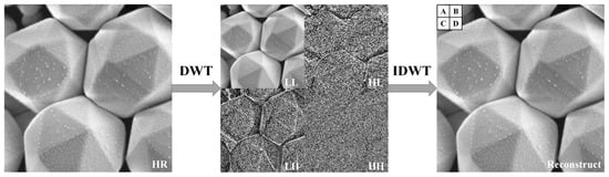
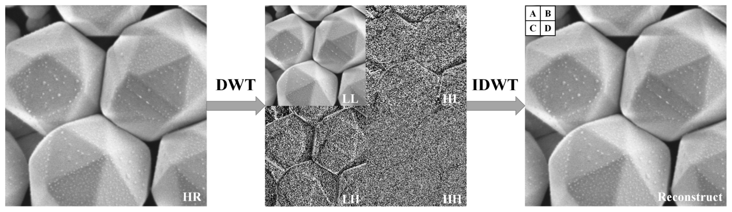
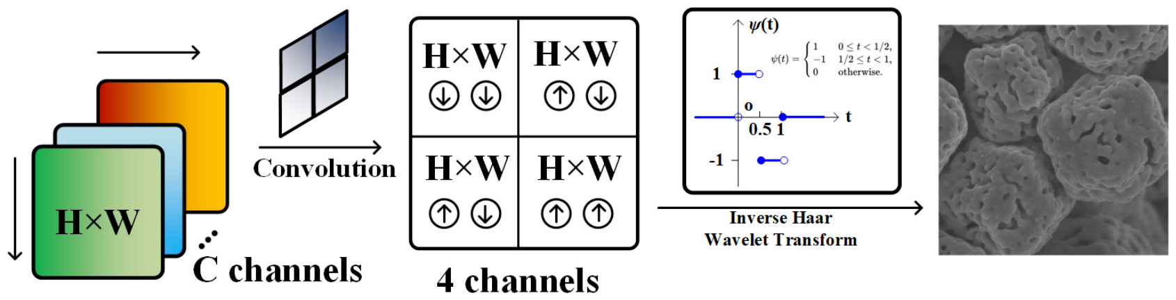
Wavelet transform has the ability to extract useful information from the signal; the wavelet transform decomposition of a signal reflects its low-frequency and high-frequency components [36]. When applying the 2D discrete wavelet transform (DWT) to the image, it can also decompose the image to its low-frequency and high-frequency components. Therefore, as a traditional image processing technique, the 2D DWT is widely used for image analysis. The input image first goes through a low-pass filter and a high-pass filter along the columns, and then goes through the low-pass filter and the high-pass filter along rows. Finally, the output of the 2D DWT consists of four coefficients denoted as $\{LL,HL,LH,HH\}$ which are all one-fourth of the number of pixels in the input image. Correspondingly, the 2D inverse DWT (IDWT) can reconstruct the four coefficients back to the input image (Figure 3).

Figure 3. (Left) The original SEM image. (Middle) 2D DWT composition (top-left for LL, top-right for HL, bottom-left for LH, bottom-right for HH) of the SEM image. (Right) IDWT reconstructed image. A, B, C, D are four pixels located in the top-left 2 × 2 grid of the reconstructed image.

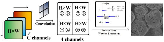
Inspired by this, we proposed a novel upscaling method for the SR task which is named as Wavelet Upscale (Figure 4). Wavelet Upscale consists of a convolutional layer and the IDWT. The output of the deep feature extraction module $I_{DF}$ first goes through a convolutional layer; the feature maps are convolved into the prediction of the four coefficients $I_{coef}=\{LL,HL,LH,HH\}$ (10):

$$I_{coef}=Conv\left(I_{DF}\right)\in R^{H\times W\times 4}$$

(10)

Figure 4. The framework of the Wavelet Upscale.

Then the prediction of the four coefficients $I_{coef}$ can be reconstructed into the SR image (11):

$$I_{SR}=IDWT\left(I_{coef}\right)=F_{WU}\left(I_{DF}\right)\in R^{2H\times 2W}$$

(11)

For the IDWT in Wavelet Upscale, we use the Haar wavelets as the core algorithm (12):

$$\left\{\begin{array}{c}A=LL+HL+LH+HH\hfill \\ B=LL-HL+LH-HH\hfill \\ C=LL+HL-LH-HH\hfill \\ D=LL-HL-LH+HH\hfill \end{array}\right.$$

(12)

The Haar wavelet is reversible; as long as the prediction of the four coefficients is accurate enough, we can reconstruct the HR image without losing accuracy (13).

$$\begin{array}{c} \mid I_{HR}-IDW{T}_{Haar}\left(DW{T}_{Haar}\left(I_{HR}\right)\right){\mid }_{l_1}<ϵ\hfill \\ ϵ=1\times {10}^{-7}\hfill \end{array}$$

(13)

The feature extraction of WLSR has a clear significance by using Wavelet Upscale as the up-sampling module, which is to predict the low-frequency and the high-frequency components of the HR image through the LR image. Wavelet Upscale has fewer parameters and less floating point operations (FLOPs) compared to other up-sampling modules, and we can perform knowledge distillation through Wavelet Upscale to enhance the performance of WLSR; we will discuss this in detail in the following section.

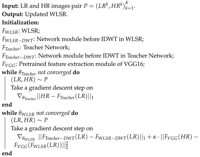
It should be noted that in fast-scan SEM images, the high-frequency subbands (HL, LH and HH) contain not only the true high-frequency surface topography of the specimen (edges, boundaries and texture) but also the shot noise introduced by the reduced dwell time. WLSR avoids amplifying the noise component in these subbands for the following reasons. First, the network is trained with paired fast-/slow-scan images of the same field of view, so it learns a conditional mapping from the noisy fast-scan input to the clean slow-scan target; the stochastic noise component cannot be predicted from the input and is therefore suppressed rather than reproduced [37]. Second, the channel–spatial attention blocks adaptively rescale the feature channels and spatial positions, which down-weights the feature responses dominated by noise. Third, and most importantly, the wavelet distillation loss supervises each subband coefficient of WLSR with the coefficient predicted by the teacher network, which is anchored to the clean slow-scan HR images (Algorithm 1); the supervision of the HL, LH and HH subbands therefore drives the predicted coefficients towards the true high-frequency structure instead of noise. Finally, the IDWT itself is a linear and invertible operator (Equation (12)) and does not amplify any frequency component; the noise behavior of WLSR is entirely determined by what the network predicts for the four coefficient maps.   

Algorithm 1: Training process of WLSR

2.2. WLSR Loss Function

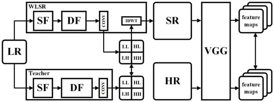
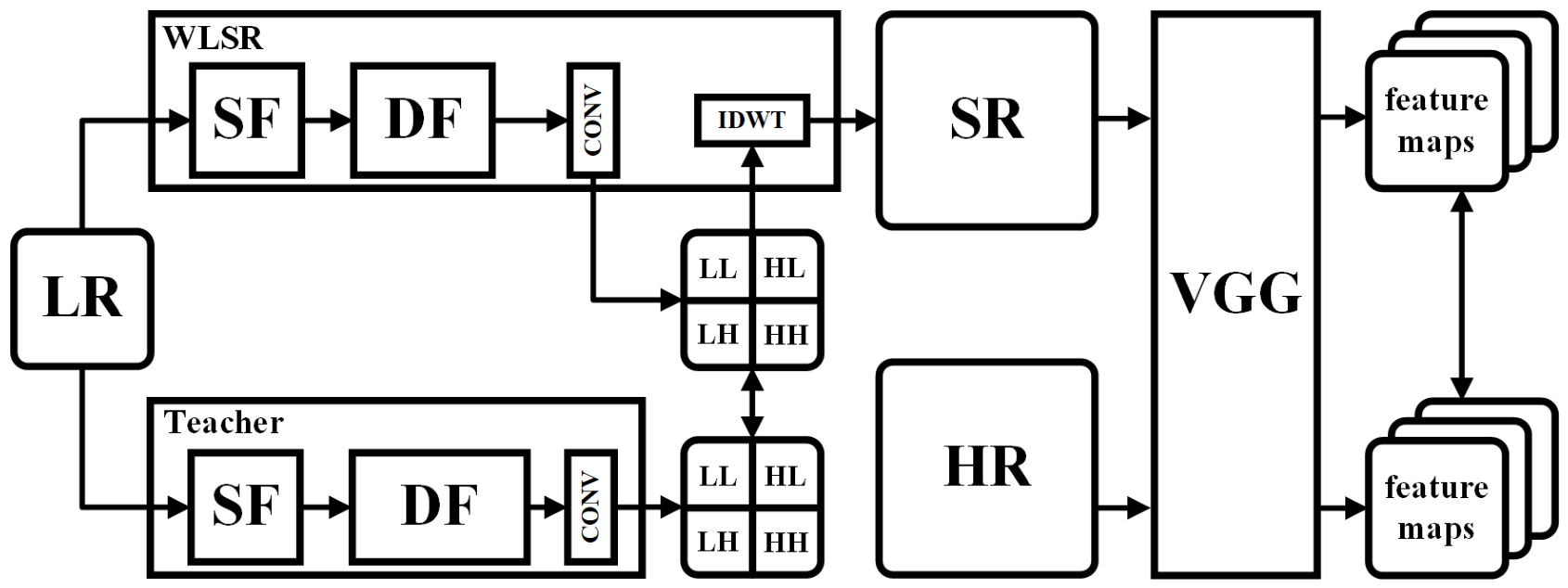
In this work, we propose a loss function that includes the wavelet distillation loss and the perceptual loss. Calculating the MAE loss between SR images and HR images is a classic scheme for SR network training. However, using the MAE loss alone for SR network training can lead to the over-smooth problem and generate images that lack detail [38]. Therefore, we introduce the wavelet distillation loss and the perceptual loss for our loss function. A larger SR network (we call it the teacher network in the following description) can generate better SR images. Through the wavelet distillation loss, we provide supervisory information across different frequency bands to WLSR. The perceptual loss can greatly improve the subjective visual quality while slightly reducing PSNR. The diagram of our loss function is shown in Figure 5. The training process of WLSR is outlined in Algorithm 1. We optimize the parameters of WLSR by minimizing our loss function $\mathcal{L}$ (14). ${\mathcal{L}}_{Wavelet}$ and ${\mathcal{L}}_{Perceptual}$ denote the wavelet distillation loss and the perceptual loss, respectively; $\alpha$ represents the coefficient used to balance different aspects of the loss. Using our loss function, WLSR can generate SR images with better details and better subjective visual quality.

$$\mathcal{L}={\mathcal{L}}_{Wavelet}+\alpha ·{\mathcal{L}}_{Perceptual}$$

(14)

Figure 5. Our loss function.

Although Equation (14) does not contain an explicit pixel-wise spatial reconstruction term, the global contrast and the intensity scale of the SR images are preserved through three mechanisms. (i) The wavelet distillation loss is computed on the four DWT coefficient maps $\{LL,HL,LH,HH\}$; the LL subband carries the low-frequency intensity and contrast information of the image, so matching the LL coefficients constrains the global intensity scale of the reconstruction. (ii) The coefficients of the teacher network are anchored to the HR ground truth through its $L_1$ pretraining (Algorithm 1), so the distillation loss indirectly couples the spatial reconstruction of WLSR to the HR reference rather than to an arbitrary target. (iii) The perceptual loss is computed between the VGG features of the SR output and those of the HR ground truth (rather than those of the teacher output), which provides an additional spatial-domain constraint to the HR reference. As shown in the ablation study, this combination yields competitive PSNR and SSIM while preserving high-frequency details, without introducing the over-smoothing that a strong additional pixel-wise reconstruction term would cause.

2.2.1. Wavelet Distillation Loss

We introduce the wavelet distillation loss into our loss function. We use a large version of WLSR as the teacher network, where the teacher network contains 180 CSABs, while WLSR contains 9 CSABs. We present the wavelet distillation loss based on knowledge distillation; by minimizing the $L1$ distance between the four coefficients $\{LL,HL,LH,HH\}$ predicted by the teacher network and those predicted by WLSR, we can improve the prediction ability of WLSR in different frequency bands. Given a number of N pairs of LR and HR images, the wavelet distillation loss ${\mathcal{L}}_{wavelet}$ can be written as (15), where $F_{WLSR-DWT}(·)$ and $F_{Teacher-DWT}(·)$ denote the network modules before IDWT in WLSR and the pretrained network module before IDWT in the teacher network, respectively:

$${\mathcal{L}}_{wavelet}={\displaystyle \frac{1}{N}}{\displaystyle \sum _{i=1}^N}\left|\right|F_{Teacher-DWT}\left(LR\right)-F_{WLSR-DWT}\left(LR\right){\left|\right|}_1$$

(15)

A potential concern is that the teacher network itself is pretrained with the $L_1$ loss (Algorithm 1), which is known to produce over-smoothed outputs. We argue that the teacher can still transfer sharp high-frequency features effectively to the student for the following reasons. First, the $L_1$ criterion is applied against the HR ground truth of the same field of view, whose optimum is the conditional median rather than the conditional mean of the pixel distribution; it therefore preserves edge locations much better than the $L_2$ criterion, and the over-smoothing of $L_1$-trained networks is considerably milder [37]. Second, over-smoothing is aggravated when the network capacity is insufficient to fit the high-frequency components of the target; the teacher contains 180 CSABs and thus possesses enough capacity to represent the high-frequency structure of the HR images. Third, the wavelet distillation loss matches the four subband coefficients separately instead of the raw pixels, which explicitly separates the high-frequency HL, LH and HH subbands from the dominant low-frequency energy and prevents the high-frequency supervision from being diluted. Finally, the perceptual loss in Equation (14) further restores the fine details that may be attenuated by the teacher, as verified by the ablation study and the feature-map visualization.

2.2.2. Perceptual Loss

We introduce the perceptual loss into our loss function. The perceptual loss can greatly improve the subjective visual quality of SR images while only slightly reducing PSNR. Given N pairs of LR and HR images, the perceptual loss ${\mathcal{L}}_{Perceptual}$ can be written as (16), where $F_{WLSR}(·)$ denotes WLSR and $F_{VGG}(·)$ denotes the pretrained feature extraction module of VGG16 [39]:

$${\mathcal{L}}_{Perceptual}={\displaystyle \frac{1}{N}}{\displaystyle \sum _{i=1}^N}\left|\right|F_{VGG}\left(HR\right)-F_{VGG}\left(F_{WLSR}\left(LR\right)\right){\left|\right|}_2^2$$

(16)

2.3. Datasets and Training Details

Datasets. The studies were conducted using an SEM (SU70, Hitachi, Tokyo, Japan). We acquired SEM images in fast and slow scanning modes of AgCl@Ag test specimens as the raw data for our SR tasks. All LR images were acquired in the fast scanning mode, which makes them inherently noisy, and each HR reference was acquired in the slow scanning mode from the same field of view; the SR task in this work therefore inherently couples image denoising with detail recovery. Subsequently, we split and cropped these images, utilizing SEM image patches for the training set and the test set. We acknowledge that the test sets contain 24 (X2) and 12 (X4) patches, which is a limited sample size for statistical analysis; all metrics reported in this paper are computed over the entire test set, and this limitation is further discussed in Section 4. The specific information of the datasets is shown in Table 1.

Table 1. Specific information of the dataset.

Dataset	Scale	The Number of	Fast Scanning Mode	Slow Scanning Mode
		Image/Patches	(Pixels/Image)	(Pixels/Image)
Raw Data	2	44	640 × 480	1280 × 960
	4	16	640 × 480	2560 × 1920
Training Set	2	2400	64 × 64	128 × 128
	4	840	64 × 64	256 × 256
Test Set	2	24	256 × 256	512 × 512
	4	12	256 × 256	1024 × 1024

Training Settings. We use the Adam optimizer with ${\beta }_1=0.9$, ${\beta }_2=0.999$ to train WLSR. The learning rate is initialized as ${10}^{-4}$ and reduced by half every 200 epochs for 1000 epochs totally. The mini-batch size is 16.

Evaluation Metrics. For the evaluation of network performance, in order to comprehensively evaluate the quality of SR images, in addition to the usual objective evaluation metrics PSNR and SSIM, we also use LPIPS [34] and FID [35] to evaluate the subjective visual quality and image style similarity. For the evaluation of network weight, we compare the parameters, FLOPs and the running time (RT). All the models were tested on an NVIDIA Quadro GV100 graphics processing unit (GPU).

3. Results

3.1. WLSR Optimization Experiment

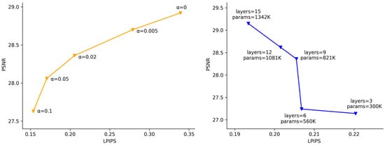
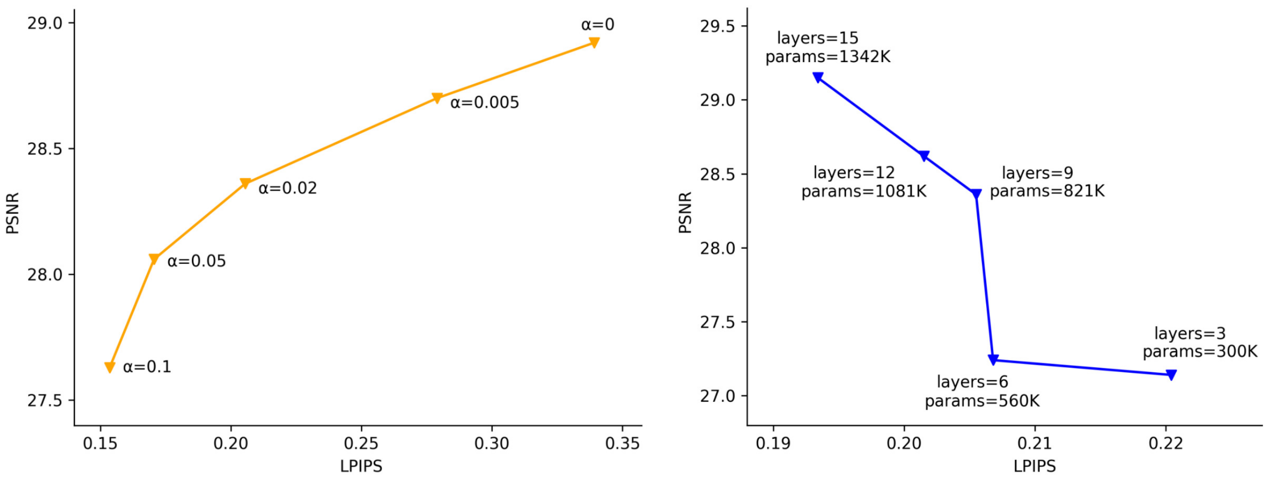
We perform an optimization experiment for the loss coefficient $\alpha$, which is also a trade-off study of PSNR vs. LPIPS. As shown in Figure 6, the perceptual loss can effectively improve the subjective visual quality and image style similarity, which is reflected in the improvement of LPIPS and FID, but also leads to a decrease of PSNR and SSIM. By optimizing the loss coefficient $\alpha$, in order to best balance the subjective visual quality and objective evaluation metrics, we finally set $\alpha =0.02$.

Figure 6. Optimization experiment for the loss coefficient $\alpha$ (left); optimization experiment for the layer number of WLSR (right).

At the same time, we perform an optimization experiment for the layer number of WLSR. As shown in Figure 6, as the number of WLSR network layers increases, the performance (PSNR and LPIPS) of WLSR improves. However, the weight (parameters) of WLSR also increase rapidly. To best balance the performance and the weight of WLSR, we finally set the layer number to 9.

3.2. WLSR Ablation Study

Then, we perform an ablation study of the network structure and a loss function analysis. For the network structure ablation study, we validate the effectiveness of the channel attention, the spatial attention and their combination, respectively. For the loss function analysis, we explored the performance of WLSR trained under the MAE loss, the wavelet distillation loss and the wavelet distillation loss with the perceptual loss, respectively. The experimental results are shown in Table 2. From Table 2, we can find out that both channel attention and spatial attention lead to performance improvement (SA: PSNR: +0.13 dB, SSIM: +0.0018; CA: PSNR: +0.75 dB, SSIM: +0.0072) and using channel–spatial attention leads to a huge performance improvement (PSNR: +1.37 dB, SSIM: +0.0223), which proves the effectiveness of the CSAB. Compared to simply using the MAE loss, using the wavelet distillation loss alone also brings considerable performance improvements (PSNR: +0.24 dB, SSIM: +0.0117). The wavelet distillation loss can provide supervisory information of different frequency bands rather than pixel supervisory information of the whole image. Although adding the perceptual loss to the wavelet distillation loss will reduce PSNR ($-0.56$ dB) and SSIM ($-0.016$), it will greatly improve the subjective visual quality and image style similarity of the image, which is reflected in LPIPS and FID (LPIPS: $-0.1336$, FID: $-7.39$).

Table 2. Ablation study of the network structure & loss function analysis. SA denotes the spatial attention, CA denotes the channel attention, WD denotes the wavelet distillation loss and P denotes the perceptual loss.

Network Structure			Loss Function				Performance
SA	CA		MAE	WD	P		PSNR (↑)	SSIM (↑)	LPIPS (↓)	FID (↓)
			✓				27.31	0.6961	0.3584	21.67
✓			✓				27.44	0.6979	0.3575	21.20
	✓		✓				28.06	0.7033	0.3422	15.51
✓	✓		✓				28.68	0.7184	0.3183	13.24
✓	✓			✓			28.92	0.7301	0.3391	16.29
✓	✓			✓	✓		28.36	0.7141	0.2055	8.90

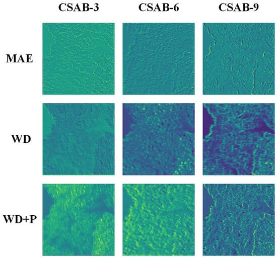
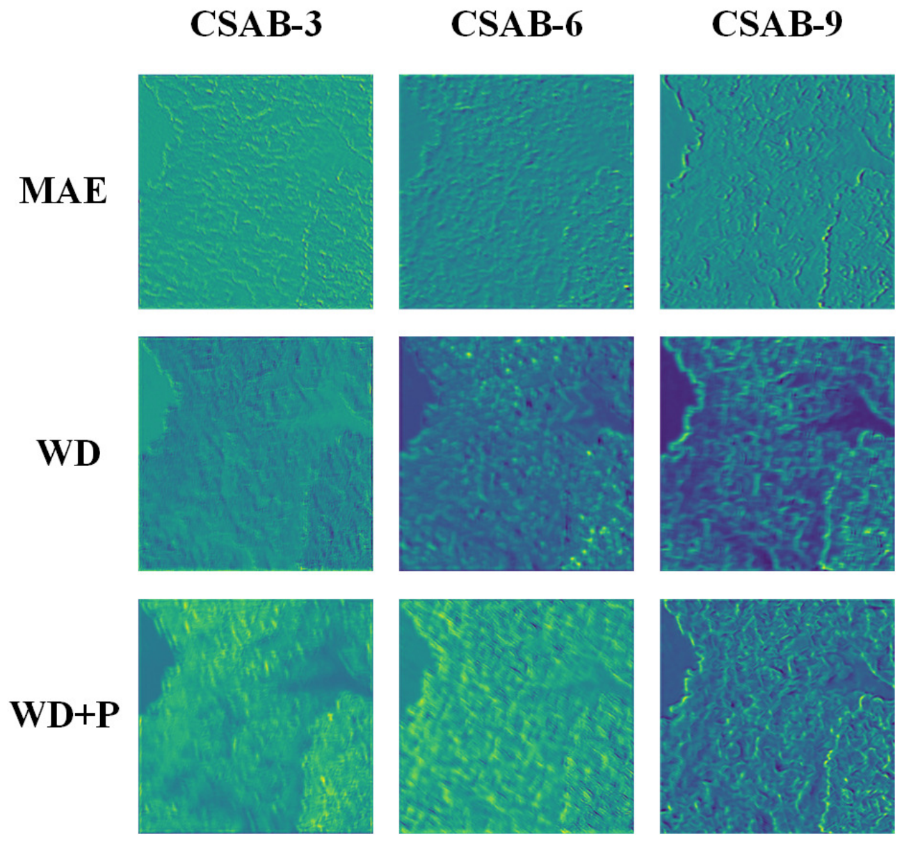
Finally, we visualized the feature maps of the middle layer of WLSR. We chose the feature maps of CSAB-3, CSAB-6 and CSAB-9 for visualization and compared WLSR with the MAE loss, the wavelet distillation loss and our final total loss (the wavelet distillation loss combined with the perceptual loss). From Figure 7 we can see that, with the gradual optimization of the WLSR loss, it pays more and more attention to the location of high-frequency detail information, thus improving the detail information recovery of fast scanning mode SEM images.

Figure 7. The visualization of WLSR’s feature maps. Rows show the output feature maps of WLSR trained with different loss functions (from top to bottom: MAE loss, wavelet distillation loss (WD), and WD combined with the perceptual loss (P)); columns show the feature maps of CSAB-3, CSAB-6 and CSAB-9, respectively. As the loss function is progressively optimized, the feature maps increasingly concentrate on the regions of high-frequency detail information (particle edges and boundaries), which explains the improved detail recovery of fast-scan SEM images.

3.3. Model Comparison

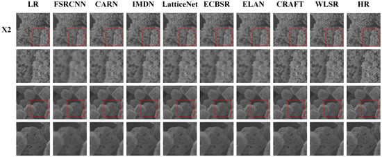
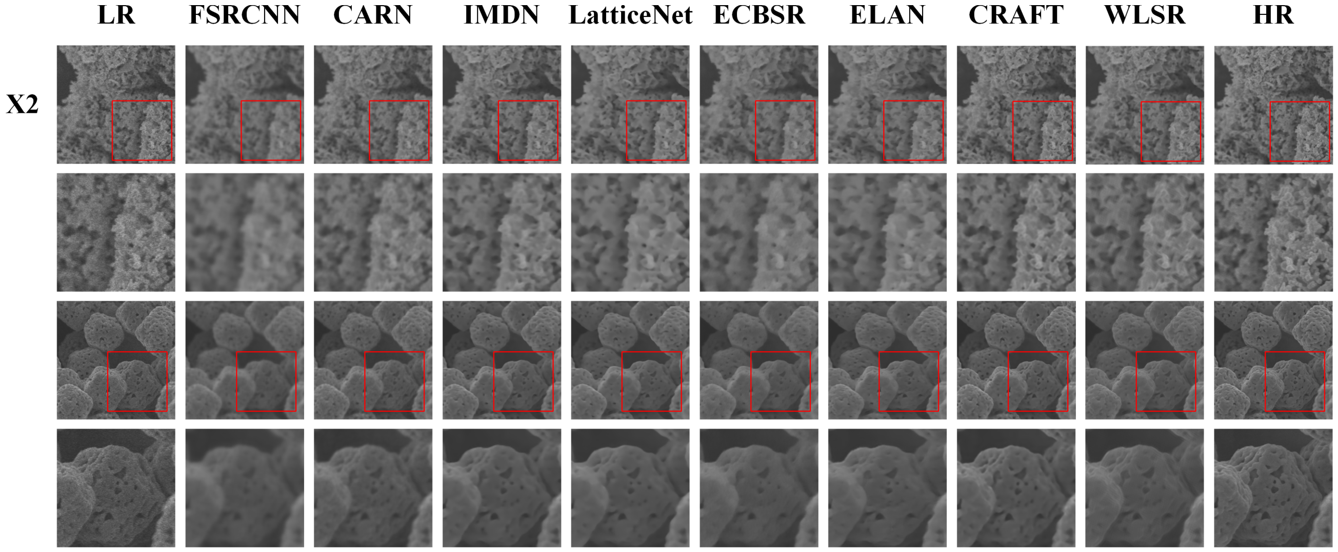
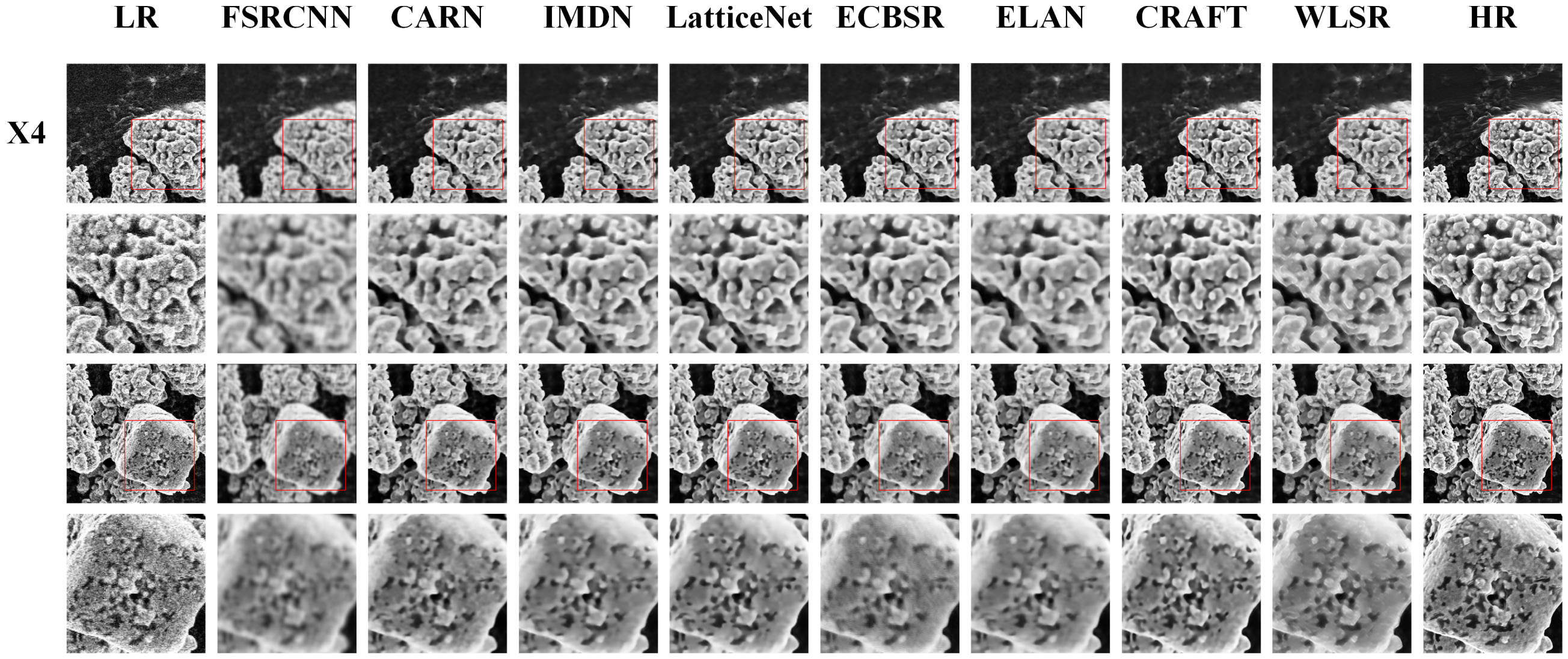
In this section, we compare WLSR with existing lightweight SR networks: FSRCNN [21], CARN [22], IMDN [23], LatticeNet [8], ECBSR [9], ELAN [10] and CRAFT [7]. We compared both X2 and X4 SR. For X4 SR, we incorporated an X2 pixelshuffle module in WLSR. The quantitative comparisons are shown in Table 3. When comparing with all given networks, WLSR provides competitive objective evaluation metrics and superior subjective visual quality. For reference, we additionally report the Bicubic interpolation baseline in Table 3, i.e., the raw fast-scan LR inputs digitally upsampled to the size of the HR references without any learned enhancement; its PSNR and SSIM quantify the absolute quality gap between the fast-scan inputs and the slow-scan HR references, and thus anchor the absolute level of enhancement achieved by each network. We emphasize that all LR inputs in Table 3 and Figure 8 and Figure 9 are raw fast-scan images acquired at a high scan speed, which contain intrinsic shot noise and jagged scan lines; the comparison therefore reflects the joint denoising and SR capability of each network on images that actually require enhancement, rather than the enhancement of already clean images. The visualization results of different lightweight SR networks are shown in Figure 8 and Figure 9. From Figure 8 and Figure 9, we can see that most other lightweight networks suffer from the over-smoothing problem and cannot provide sufficient high-frequency details. WLSR, by utilizing the wavelet distillation loss and the perceptual loss, can provide more high-frequency detail information and better subjective visual quality with competitive objective evaluation metrics.

Table 3. Model comparison of different lightweight SR networks on super-resolving SEM images.

Model	Scale	Performance					Weight of Model
		PSNR (↑)	SSIM (↑)	LPIPS (↓)	FID (↓)		Params (↓)	FLOPs (↓)	RT (↓)
Bicubic	2 2	25.81	0.6423	0.5871	67.32		–	–	–
FSRCNN		27.18	0.6956	0.4906	41.19		13 K	2.5 G	0.7 ms
CARN		28.36	0.7109	0.3806	18.17		1590 K	296.5 G	4.6 ms
IMDN		28.39	0.7179	0.3426	16.66		689 K	210.6 G	4.1 ms
LatticeNet		27.96	0.7077	0.3420	19.83		750 K	225.3 G	7.4 ms
ECBSR-M16C64		27.25	0.6938	0.2702	16.11		596 K	183.1 G	53.9 ms
ELAN-Light		27.49	0.6963	0.3176	16.75		577 K	178.0 G	178.1 ms
CRAFT		27.10	0.6787	0.3267	11.64		733 K	131.5 G	302.1 ms
WLSR		28.36	0.7141	0.2055	8.90		821 K	250.8 G	3.7 ms
Bicubic	4 4	16.42	0.3615	0.9214	132.76		–	–	–
FSRCNN		18.13	0.4088	0.8421	104.35		13 K	2.5 G	0.7 ms
CARN		19.46	0.4509	0.7801	59.84		1590 K	480.5 G	6.1 ms
IMDN		18.73	0.4314	0.7483	57.40		696 K	212.7 G	4.1 ms
LatticeNet		19.02	0.4391	0.7477	53.85		757 K	227.4 G	7.4 ms
ECBSR-M16C64		18.70	0.4220	0.6006	40.59		603 K	185.2 G	54.8 ms
ELAN-Light		18.67	0.4277	0.6748	60.70		583 K	180.0 G	179.5 ms
CRAFT		18.71	0.4402	0.7438	49.60		739 K	133.1 G	302.1 ms
WLSR		18.98	0.4260	0.4835	26.71		969 K	298.3 G	3.9 ms

Figure 8. Visual comparisons of different lightweight SR networks on X2 super-resolution of SEM images. Two representative test fields are shown; in each group, the upper row shows the full field of view in which the red boxes mark the zoom regions, and the lower row shows the corresponding zoomed patches. All LR inputs are raw fast-scan images.

Figure 9. Visual comparisons of different lightweight SR networks on X4 super-resolution of SEM images. Two representative test fields are shown; in each group, the upper row shows the full field of view in which the red boxes mark the zoom regions, and the lower row shows the corresponding zoomed patches. All LR inputs are raw fast-scan images.

4. Discussion

The results of this study show that WLSR provides a practical solution to the long-standing trade-off in SEM observation between imaging speed and image quality. In the network structure, the channel–spatial attention block enables the network to concentrate its limited computational resources on the most informative feature channels and spatial locations, while the Wavelet Upscale reformulates upscaling as the prediction of the low-frequency and high-frequency wavelet coefficients of the HR image. The proposed loss function further exploits this frequency-domain formulation: the wavelet distillation loss transfers frequency-band-level supervisory information from a deep teacher network (180 CSABs) to WLSR (9 CSABs), and the perceptual loss preserves the high-frequency details that the MAE loss tends to smooth out [38]. The ablation study confirms that these components are complementary, and the optimization experiments show that the loss coefficient $\alpha$ allows an explicit trade-off between objective fidelity (PSNR/SSIM) and perceptual quality (LPIPS/FID); $\alpha =0.02$ was selected to balance the two aspects.

Compared with existing lightweight SR networks, deep and perceptual models developed for SEM super-resolution are typically too heavy for real-time deployment [24,29,30], while several transformer-based lightweight networks achieve competitive PSNR but require 178.1 ms (ELAN-Light) and 302.1 ms (CRAFT) per image, respectively (Table 3), which prevents their use during live SEM observation. In contrast, WLSR super-resolves a fast scanning mode image in only 3.7 ms on an NVIDIA Quadro GV100 GPU, which is far shorter than the acquisition time of a fast-scan frame, so that the inference speed is compatible with live SEM observation. It should be emphasized, however, that all results in this work were obtained by processing pre-acquired images offline, and WLSR has not yet been integrated into the live acquisition pipeline of an SEM; the “digital objective lens” should therefore be understood as the design goal of the proposed framework rather than a description of a finished software product. In this sense, WLSR is expected to behave as a “digital objective lens”: low-magnification fast scans would be displayed as digitally magnified 2× or 4× images of slow-scan quality in real time, so that HR observation no longer requires switching to the slow scanning mode. Integrating WLSR into the SEM console (e.g., through the image acquisition interface of the microscope, with a GPU workstation) and verifying the end-to-end latency during live observation is the focus of our ongoing work.

This capability is expected to benefit process-level observation, in which the evolution of surface morphology during material processing must be tracked continuously, as well as high-throughput materials characterization. It should be noted that this value is not merely a matter of saving the switching time: in in-situ and process-level observation the specimen state evolves continuously and cannot be revisited afterwards, so a slow scan acquired minutes later would image a different state; in high-throughput workflows the per-field switching cost accumulates over large numbers of fields; and for beam-sensitive specimens a single low-dose fast frame enhanced by WLSR avoids the concentrated electron dose of a slow scan. In future work, we will combine WLSR with fast scanning mode video recording and lightweight detection models to realize fully automated “SEM Mapping” for wide-range, real-time material characterization.

Limitations and Future Work

Several limitations of this work should be acknowledged, which also define our future research directions.

First, the network was trained and evaluated on AgCl@Ag particulate specimens. The secondary-electron yield, surface charging behavior and beam sensitivity differ substantially across material classes, and the performance of WLSR on non-particulate, non-crystalline or heterogeneous materials (e.g., biological tissue, polymers and beam-sensitive organic substances) has not been systematically evaluated. The framework itself is material-agnostic: the paired fast-/slow-scan data required for training can be acquired for any specimen that withstands the slow-scan acquisition, and both the channel–spatial attention and the wavelet decomposition operate on the image signal rather than on material-specific assumptions. Charging artifacts, however, mainly manifest as low-frequency intensity shifts and local brightness distortions, which partially violate the one-to-one correspondence between the fast- and slow-scan images of the same field of view; severe charging should therefore be suppressed at the acquisition stage (e.g., by charge compensation, a lower accelerating voltage or low-vacuum mode), and the network can only be expected to compensate the mild charging represented in its training data. For beam-sensitive materials, for which the slow-scan HR reference is difficult to acquire because the specimen is damaged or altered by the slow scan itself, we see three feasible routes to obtain training data. (i) Self-supervised training: following the Noise2Noise principle [37], several independent fast scans of the same field of view share the same underlying signal while their noise realizations are statistically independent, so a network can learn to restore one noisy fast scan from another without any slow-scan HR image. (ii) Frame averaging: the average of K independent fast scans converges to a low-noise image that can serve as a surrogate HR reference; the total electron dose equals that of the K fast scans and is fractionated over time, which mitigates damage accumulation. (iii) Synthetic degradation pretraining: WLSR can first be trained on HR images with simulated fast-scan degradation (noise and resolution attenuation calibrated on our paired data) and then fine-tuned with a small real paired set from the target material. We emphasize that acquiring training data is a one-time, offline cost per material class, whereas the trained WLSR then provides instantaneous enhancement of every subsequent fast scan during live observation; this asymmetric cost is precisely the scenario in which a “digital objective lens” is profitable.

Second, systematic robustness tests against dynamic SEM anomalies—sample charging, beam drift and line jitter—have not been performed. Mild instances of these artifacts occur naturally in our fast-scan training data, so the network has been exposed to them to a limited extent; however, extreme beam drift or line jitter may break the pixel-level correspondence between the LR and HR patches. Data augmentation with simulated drift and jitter, together with an online quality-monitoring module that flags inputs outside the training distribution, will be studied to improve robustness.

Third, the evaluation in this work relies on pixel-based and perceptual metrics (PSNR, SSIM, LPIPS and FID), which do not directly measure physical quantities. For materials-science applications, the SR results should additionally be validated with physical metrology, such as grain-size statistics, edge-spread-function-based edge width measurements and line-edge roughness analysis, as demonstrated for quantification purposes in [29]. A physical-metrology-based validation on specimens with calibrated feature sizes is planned as future work.

A further open question is the minimum input quality that WLSR can tolerate. All LR images used in this work were acquired with the fast scanning settings of the same instrument, which represent the practical lower bound of the input quality tested so far; when the noise level of the input departs significantly from the training distribution, the network may produce hallucinated texture or residual noise, because the learned prior is only valid near the training distribution. We plan to characterize this boundary by synthetically degrading the test inputs with controlled noise levels (e.g., Poisson–Gaussian noise calibrated to a series of target signal-to-noise ratios), sweeping the input SNR and recording the output PSNR, SSIM and LPIPS, so as to determine the minimum input SNR below which processing artifacts become unacceptable, and to extend this range by retraining with heavier data augmentation.

Finally, the test sets consist of 24 (X2) and 12 (X4) patches, which is statistically limited; the reported metrics should be interpreted as indicative rather than as definitive population estimates. We will expand the evaluation to larger, multi-material test sets, including extremely low-beam-current fast scans, to further verify the reliability and generalization of WLSR.

5. Conclusions

In this work, we proposed WLSR, a wavelet-based lightweight SR network designed to narrow the quality gap between fast- and slow-scan SEM imaging. The network combines channel–spatial attention blocks for efficient feature selection with a Wavelet Upscale module that formulates upscaling as the prediction of the four wavelet coefficient maps of the HR image; it is trained with a novel loss function in which the wavelet distillation loss transfers frequency-band-level supervision from a deep teacher network to the lightweight student, and the perceptual loss restores the high-frequency details that the pixel-wise MAE loss tends to smooth out. On paired fast-/slow-scan SEM images of AgCl@Ag specimens, WLSR achieved a competitive PSNR of 28.36 dB and SSIM of 0.7141, together with the best LPIPS (0.2055) and FID (8.90) among eight lightweight SR networks in the X2 task, while running at 3.7 ms per image on an NVIDIA Quadro GV100 GPU; in the X4 task, it likewise provided the best perceptual quality with a competitive inference speed. Because the inference time is far shorter than the acquisition time of a fast-scan frame, WLSR can potentially serve as a “digital objective lens” that displays digitally magnified, slow-scan-quality images in real time during fast scanning. We emphasize that the current implementation processes pre-acquired images offline, and its generalization to other material classes, its robustness to extreme imaging anomalies and to inputs near the minimum tolerable signal-to-noise ratio, and a physical-metrology-based validation remain to be established. These aspects, together with the integration of WLSR into the live SEM acquisition pipeline and its combination with fast-scan video recording and lightweight detection models for fully automated “SEM Mapping”, constitute our future work.

References

- Goldstein, J.I.; Newbury, D.E.; Michael, J.R.; Ritchie, N.W.; Scott, J.H.J.; Joy, D.C. Scanning Electron Microscopy and X-Ray Microanalysis, 4th ed.; Springer: New York, NY, USA, 2018. [Google Scholar]
- Schatten, H. Low voltage high-resolution SEM (LVHRSEM) for biological structural and molecular analysis. Micron 2011, 42, 175–185. [Google Scholar] [CrossRef] [Scilit] [PubMed]
- Pelton, W.R. Distinguishing the cause of textile fiber damage using the scanning electron microscope (SEM). J. Forensic Sci. 1995, 40, 874–882. [Google Scholar] [CrossRef] [Scilit]
- Sun, N.; Jia, Y.; Bai, S.; Yang, Y.; Dai, L.; Li, J. Spatial mapping and quantitative evaluation of protein corona on pegylated mesoporous silica particles by super-resolution fluorescence microscopy. J. Colloid Interface Sci. 2024, 653, 351–358. [Google Scholar] [CrossRef] [Scilit] [PubMed]
- Kajner, G.; Galbács, G. Exploring the Use of Nanoporous Glass Substrates for the Quantitative Trace Microanalysis of Aqueous Samples by Surface-Enhanced Laser-Induced Breakdown Spectroscopy. Anal. Chem. 2025, 97, 12000–12004. [Google Scholar] [CrossRef] [Scilit] [PubMed]
- Akbari Dana, P.; Gaga, E.O.; Gedik, K. Analytical Challenges and Strategies for Particle-Based Analysis of Airborne Micro (nano) plastics in Size-Fractionated Samples Using Microscopy, SEM/EDX, and Raman Spectroscopy. Anal. Chem. 2024, 96, 20622–20634. [Google Scholar] [CrossRef] [Scilit] [PubMed]
- Li, A.; Zhang, L.; Liu, Y.; Zhu, C. Feature modulation transformer: Cross-refinement of global representation via high-frequency prior for image super-resolution. In Proceedings of the IEEE/CVF International Conference on Computer Vision, Paris, France, 1–6 October 2023; pp. 12514–12524. [Google Scholar]
- Luo, X.; Xie, Y.; Zhang, Y.; Qu, Y.; Li, C.; Fu, Y. Latticenet: Towards lightweight image super-resolution with lattice block. In Proceedings of the European Conference on Computer Vision; Springer: Cham, Switzerland, 2020; pp. 272–289. [Google Scholar]
- Zhang, X.; Zeng, H.; Zhang, L. Edge-oriented convolution block for real-time super resolution on mobile devices. In Proceedings of the 29th ACM International Conference on Multimedia; Association for Computing Machinery: New York, NY, USA, 2021; pp. 4034–4043. [Google Scholar]
- Zhang, X.; Zeng, H.; Guo, S.; Zhang, L. Efficient long-range attention network for image super-resolution. In Proceedings of the European Conference on Computer Vision; Springer: Cham, Switzerland, 2022; pp. 649–667. [Google Scholar]
- Lim, B.; Son, S.; Kim, H.; Nah, S.; Mu Lee, K. Enhanced deep residual networks for single image super-resolution. In Proceedings of the IEEE Conference on Computer Vision and Pattern Recognition Workshops, Honolulu, HI, USA, 21–26 July 2017; pp. 136–144. [Google Scholar]
- Zhang, Y.; Tian, Y.; Kong, Y.; Zhong, B.; Fu, Y. Residual dense network for image super-resolution. In Proceedings of the IEEE Conference on Computer Vision and Pattern Recognition, Salt Lake City, UT, USA, 18–23 June 2018; pp. 2472–2481. [Google Scholar]
- Zhang, Y.; Li, K.; Li, K.; Wang, L.; Zhong, B.; Fu, Y. Image super-resolution using very deep residual channel attention networks. In Proceedings of the European Conference on Computer Vision (ECCV); Springer: Cham, Switzerland, 2018; pp. 286–301. [Google Scholar]
- Kwasniewska, A.; Ruminski, J.; Szankin, M.; Kaczmarek, M. Super-resolved thermal imagery for high-accuracy facial areas detection and analysis. Eng. Appl. Artif. Intell. 2020, 87, 103263. [Google Scholar] [CrossRef] [Scilit]
- Lin, Z.; Gao, Z.; Ji, H.; Zhai, R.; Shen, X.; Mei, T. Classification of cervical cells leveraging simultaneous super-resolution and ordinal regression. Appl. Soft Comput. 2022, 115, 108208. [Google Scholar] [CrossRef] [Scilit]
- Choi, Y.J.; Kim, B.G. HiRN: Hierarchical recurrent neural network for video super-resolution (VSR) using two-stage feature evolution. Appl. Soft Comput. 2023, 143, 110422. [Google Scholar] [CrossRef] [Scilit]
- Liang, J.; Cao, J.; Sun, G.; Zhang, K.; Van Gool, L.; Timofte, R. Swinir: Image restoration using swin transformer. In Proceedings of the IEEE/CVF International Conference on Computer Vision, Montreal, BC, Canada, 11–17 October 2021; pp. 1833–1844. [Google Scholar]
- Liu, Z.; Lin, Y.; Cao, Y.; Hu, H.; Wei, Y.; Zhang, Z.; Lin, S.; Guo, B. Swin transformer: Hierarchical vision transformer using shifted windows. In Proceedings of the IEEE/CVF international conference on computer vision, Montreal, QC, Canada, 10–17 October 2021; pp. 10012–10022. [Google Scholar]
- Vaswani, A.; Shazeer, N.; Parmar, N.; Uszkoreit, J.; Jones, L.; Gomez, A.N.; Kaiser, Ł.; Polosukhin, I. Attention is all you need. In Proceedings of the 31st International Conference on Neural Information Processing Systems, Long Beach, CA, USA, 4–9 December 2017; Volume 30. [Google Scholar]
- Li, T.; Jin, X.; Liu, Q.; Liu, X. Image Super-Resolution Reconstruction Network Based on Structural Reparameterization and Feature Reuse. Sensors 2025, 25, 5989. [Google Scholar] [CrossRef] [Scilit] [PubMed]
- Dong, C.; Loy, C.C.; Tang, X. Accelerating the super-resolution convolutional neural network. In Proceedings of the Computer Vision–ECCV 2016: 14th European Conference, Amsterdam, The Netherlands, 11–14 October 2016; Proceedings, Part II 14; Springer: Cham, Switzerland, 2016; pp. 391–407. [Google Scholar]
- Ahn, N.; Kang, B.; Sohn, K.A. Fast, accurate, and lightweight super-resolution with cascading residual network. In Proceedings of the European Conference on Computer Vision (ECCV); Springer: Cham, Switzerland, 2018; pp. 252–268. [Google Scholar]
- Hui, Z.; Gao, X.; Yang, Y.; Wang, X. Lightweight image super-resolution with information multi-distillation network. In Proceedings of the 27th ACM International Conference on Multimedia; Association for Computing Machinery: New York, NY, USA, 2019; pp. 2024–2032. [Google Scholar]
- de Haan, K.; Ballard, Z.S.; Rivenson, Y.; Wu, Y.; Ozcan, A. Resolution enhancement in scanning electron microscopy using deep learning. Sci. Rep. 2019, 9, 12050. [Google Scholar] [CrossRef] [Scilit] [PubMed]
- Johnson, J.; Alahi, A.; Fei-Fei, L. Perceptual losses for real-time style transfer and super-resolution. In Proceedings of the Computer Vision–ECCV 2016: 14th European Conference, Amsterdam, The Netherlands, 11–14 October 2016; Proceedings, Part II 14; Springer: Cham, Switzerland, 2016; pp. 694–711. [Google Scholar]
- Hinton, G.; Vinyals, O.; Dean, J. Distilling the knowledge in a neural network. arXiv 2015, arXiv:1503.02531. [Google Scholar]
- Wang, J.; Lan, C.; Wang, C.; Gao, Z. Deep learning super-resolution electron microscopy based on deep residual attention network. Int. J. Imaging Syst. Technol. 2021, 31, 2158–2169. [Google Scholar]
- Fan, L.; Wang, Z.; Lu, Y.; Zhou, J. An adversarial learning approach for super-resolution enhancement based on AgCl@ Ag nanoparticles in scanning electron microscopy images. Nanomaterials 2021, 11, 3305. [Google Scholar] [CrossRef] [Scilit] [PubMed]
- Furat, O.; Finegan, D.P.; Yang, Z.; Kirstein, T.; Smith, K.; Schmidt, V. Super-resolving microscopy images of Li-ion electrodes for fine-feature quantification using generative adversarial networks. npj Comput. Mater. 2022, 8, 68. [Google Scholar] [CrossRef] [Scilit]
- Wang, Z.; Feng, R.; Mao, J.; Tao, X.; Zhang, D.; Shan, X.; Zhou, J. SRFS: Super Resolution in Fast-Slow Scanning Mode of SEM Based on Denoising Diffusion Probability Model. IEEE Trans. Instrum. Meas. 2024, 73, 5008409. [Google Scholar] [CrossRef] [Scilit]
- Ji, H.; Fermüller, C. Robust wavelet-based super-resolution reconstruction: Theory and algorithm. IEEE Trans. Pattern Anal. Mach. Intell. 2008, 31, 649–660. [Google Scholar] [CrossRef] [Scilit] [PubMed]
- Anbarjafari, G.; Demirel, H. Image super resolution based on interpolation of wavelet domain high frequency subbands and the spatial domain input image. ETRI J. 2010, 32, 390–394. [Google Scholar] [CrossRef] [Scilit]
- Mallat, S.; Yu, G. Super-resolution with sparse mixing estimators. IEEE Trans. Image Process. 2010, 19, 2889–2900. [Google Scholar] [CrossRef] [Scilit] [PubMed]
- Zhang, R.; Isola, P.; Efros, A.A.; Shechtman, E.; Wang, O. The unreasonable effectiveness of deep features as a perceptual metric. In Proceedings of the IEEE Conference on Computer Vision and Pattern Recognition (CVPR), Salt Lake City, UT, USA, 18–23 June 2018; pp. 586–595. [Google Scholar]
- Heusel, M.; Ramsauer, H.; Unterthiner, T.; Nessler, B.; Hochreiter, S. GANs trained by a two time-scale update rule converge to a local Nash equilibrium. In Proceedings of the Advances in Neural Information Processing Systems (NeurIPS), Long Beach, CA, USA, 4–9 December 2017; Volume 30, pp. 9624–9635. [Google Scholar]
- Malyugina, A.; Anantrasirichai, N.; Bull, D. Wavelet-Based Topological Loss for Low-Light Image Denoising. Sensors 2025, 25, 2047. [Google Scholar] [CrossRef] [Scilit] [PubMed]
- Lehtinen, J.; Munkberg, J.; Hasselgren, J.; Laine, S.; Karras, T.; Aittala, M.; Aila, T. Noise2Noise: Learning image restoration without clean data. In Proceedings of the International Conference on Machine Learning (ICML), Stockholm, Sweden, 10–15 July 2018; pp. 2965–2974. [Google Scholar]
- Shang, J.; Xu, Z.; Wang, D. Global-Token U-Net with Hybrid Loss for Trustworthy Medical Image Super-Resolution. Sensors 2026, 26, 1454. [Google Scholar] [CrossRef] [Scilit] [PubMed]
- Simonyan, K.; Zisserman, A. Very deep convolutional networks for large-scale image recognition. arXiv 2014, arXiv:1409.1556. [Google Scholar]
Disclaimer/Publisher’s Note: The statements, opinions and data contained in all publications are solely those of the individual author(s) and contributor(s) and not of MDPI and/or the editor(s). MDPI and/or the editor(s) disclaim responsibility for any injury to people or property resulting from any ideas, methods, instructions or products referred to in the content. |
© 2026 by the authors. Licensee MDPI, Basel, Switzerland. This article is an open access article distributed under the terms and conditions of the Creative Commons Attribution (CC BY) license.