Quantifying Pressure Propagation and Oil Mobilization Across Fracture and Matrix Regions in a Hydraulically Fractured Shale Oil Well

Highlights

What are the main findings?

• Pressure depletion propagates outward from fractures into the matrix.

• Oil expansion accounts for 61.73% of the net oil withdrawal from the matrix regions, and the stimulated matrix contributes 74.52% of the net oil withdrawal.

What are the implications of the main findings?

• Matrix permeability and retained fracture conductivity are identified as the governing factors for pressure propagation in the fractured shale oil reservoir.

Abstract

Pressure propagation and oil mobilization across fracture and matrix regions during primary depletion remain poorly quantified in hydraulically fractured shale oil wells. A history-matched compositional model of Well H2CHF (Funing Formation, Subei Basin) simulated fracturing-fluid injection, shut-in, and production. The reservoir was partitioned along the oil-flow pathway into hydraulic fractures, stimulated matrix, and unstimulated reservoir, and the net oil withdrawal of each region was apportioned among drive mechanisms by material balance. Injection raised average pressure from 51.11 MPa to 75.15 MPa in the hydraulic fractures and 63.37 MPa in the stimulated matrix. After production began, pressure depletion propagated outward, leaving final pressures of 14.88, 16.37, and 21.23 MPa in the three regions, respectively. The stimulated matrix supplied 74.52% of the cumulative net oil withdrawal, whereas the hydraulic fractures served mainly as flow pathways. The recovery factor was 9.61%. In the two matrix regions, oil expansion, pore-volume contraction, oil displacement by fracturing fluid, and solution-gas drive contributed 61.73%, 13.13%, 10.69%, and 14.45%, respectively, and solution-gas drive dominated in the stimulated matrix during low-pressure depletion. Matrix permeability and retained fracture conductivity controlled pressure propagation, while the production schedule controlled pressure depletion. These results support region-specific production scheduling and pressure-support design.

1. Introduction

Continental shale oil has become an important strategic resource for China’s onshore petroleum industry, with large-scale development accelerating in the Ordos, Junggar, and Subei basins and the Jiyang Depression [1,2,3,4]. The Second Member of the Funing Formation in the Gaoyou Sag, Subei Basin, is a typical laminated lacustrine shale oil interval that acts as both a source rock and a reservoir, and holds substantial original oil in place. Since the first well commenced production in 2022, multiple horizontal wells have been deployed in this interval [5,6,7,8]. Each well drains a relatively closed reservoir volume with little external pressure support. Recovery factors are generally below 10%, and individual wells exhibit high initial production rates followed by rapid decline [9,10]. Much of the oil remains unrecovered because stimulation-induced pressure buildup is uneven and pressure depletion propagates slowly through the drainage volume. Maximizing recovery under primary depletion therefore requires a clear understanding of how pressure evolves within each well drainage volume and where and when oil is mobilized.

Spatial heterogeneity in oil mobilization arises from the strongly nonlinear flow behavior of shale reservoirs. As effective stress increases during depletion, fracture conductivity declines rapidly, creating pronounced differences in oil deliverability between near-fracture and far-field matrix regions [11,12]. Nanopore confinement further alters oil-phase behavior and transport properties [13,14]. Nanoconfinement, stress sensitivity, threshold pressure gradients, and fracture-tip pressure differentials can interact nonlinearly and cause departures from Darcy flow in tight oil reservoirs [15,16,17,18,19]. However, most of these studies infer the behavior of the entire stimulated region from bottomhole pressure or spatially averaged reservoir properties. Such lumped-parameter approaches cannot quantify how much oil is mobilized from the hydraulic fractures, the stimulated matrix, and the unstimulated reservoir.

Temporal variations in oil mobilization arise because the relative contributions of drive mechanisms change as reservoir pressure evolves. During depletion, shale oil production is driven by elastic energy released through pore-volume contraction and fluid expansion, together with oil displacement by invading fracturing fluid [20,21]. Spontaneous imbibition of fracturing fluid into the matrix is an important recovery mechanism, and laboratory experiments have quantified the roles of capillary forces, osmotic pressure, and wettability in this process [22,23,24]. Shut-in duration controls the relative contributions of imbibition and elastic-energy release [25,26,27,28,29]. However, these studies mostly evaluate individual mechanisms at laboratory scale, and field-scale methods that partition the contributions of multiple drive mechanisms over the full pressure history remain scarce.

At field scale, Wang et al. [30] used material balance to estimate the drained rock volume (DRV) and to partition drive-mechanism contributions, building on the volume-based concepts of stimulated reservoir volume (SRV) [31] and DRV [32]. Pressure-support techniques, including water, gas, and CO₂ huff-n-puff and energy-storage hydraulic fracturing, have been applied to increase recovery from shale oil reservoirs [33,34,35,36,37,38,39]. Because reservoir pressure is a primary control on recovery factor [40,41], pressure-support operations should be designed on the basis of the pressure–mobilization relationship during depletion and the associated stress evolution [42]. However, most existing methods address bulk volume, spatial extent, or early-time matrix–fracture responses and do not combine the full pressure history with regional oil mobilization and individual drive mechanisms, which limits their use in production scheduling and pressure-support design.

To address these gaps, a compositional model of Well H2CHF in the Second Member of the Funing Formation, Gaoyou Sag, was developed for the complete sequence of fracturing-fluid injection, shut-in, and production, and was calibrated against field production data. The modeled reservoir was partitioned along the oil-flow pathway into three control regions: hydraulic fractures, stimulated matrix, and unstimulated reservoir. Average reservoir pressure, net oil withdrawal, and oil production per unit pressure decline were used to quantify pressure evolution and oil mobilization in each region. Material balance was then applied to apportion net oil withdrawal among four drive mechanisms (oil expansion, pore-volume contraction, oil displacement by fracturing fluid, and solution-gas drive) and to identify stage-dependent shifts in their relative contributions. Finally, 35 sensitivity cases were used to identify the main controls on oil mobilization in the control regions. Unlike the well-scale material balance used by Wang et al. [30] to estimate the DRV, this approach resolves pressure and oil inventory separately in fixed control regions and continuously from injection to depletion, so that the net oil withdrawal of each region can be related to its own pressure decline.

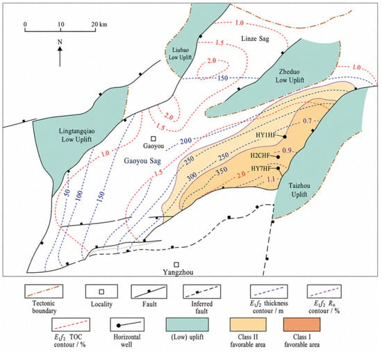
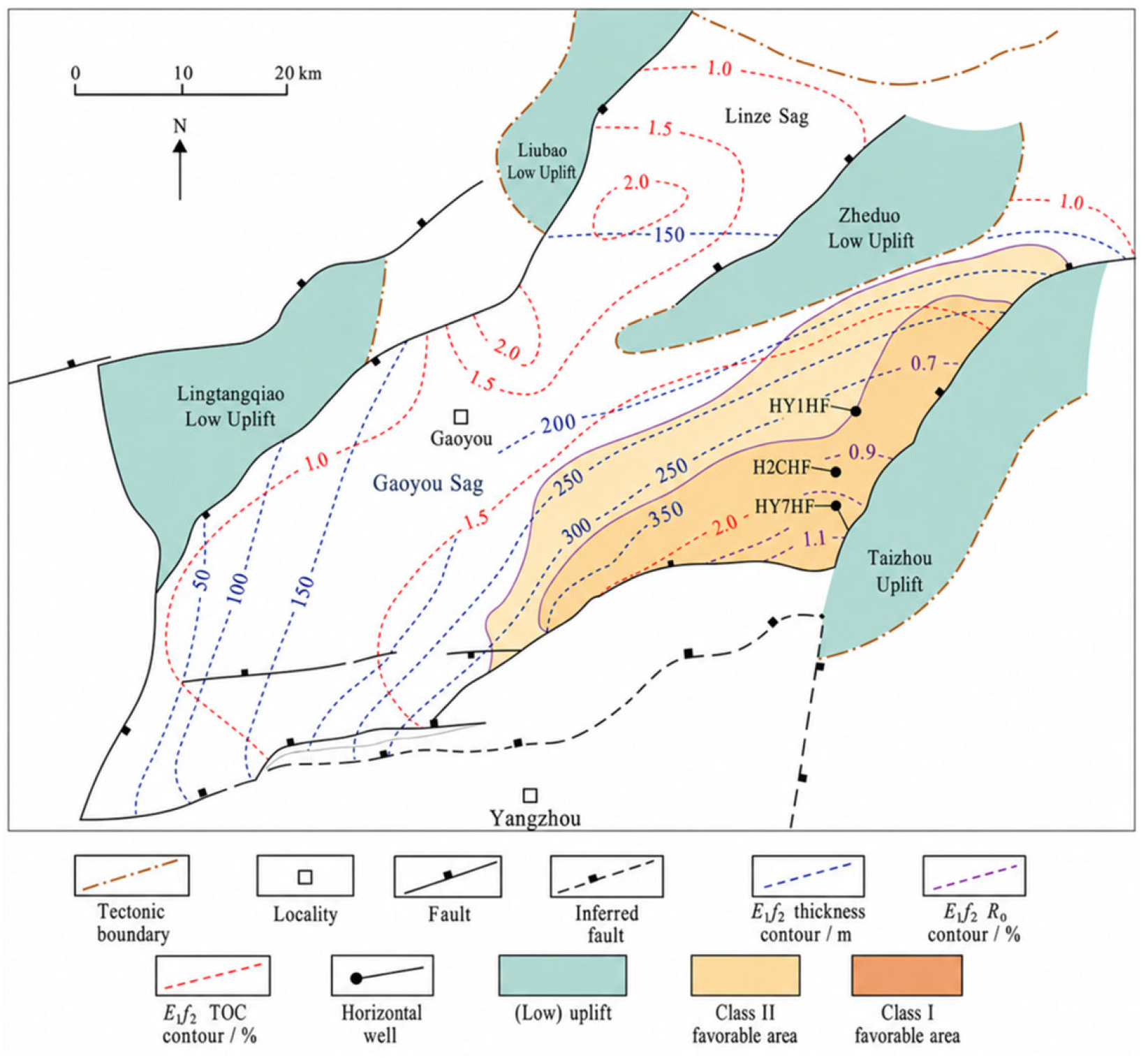
The study area is the Huazhuang area on the northern slope of the Gaoyou Sag, a northeast–southwest-trending asymmetric half-graben in the Dongtai Depression of the Subei Basin [5,6,43] (Figure 1). The target interval, the Second Member of the Paleogene Funing Formation (E₁f₂), was deposited in a semi-deep to deep lacustrine setting. It is 280–350 m thick, lies at an average burial depth of approximately 3800 m in the prospective areas, and has its principal targets in Submembers IV and V [6]. The shale has a total organic carbon (TOC) content of 0.60–1.50%, Type II₁–II₂ kerogen, and a vitrinite reflectance (R_o) of 0.50–1.10%, which places it within the oil window [5]. Approximately east–west- and northeast-trending fault sets, including microfaults, divide the thick shale succession into narrow fault blocks with complex boundaries and limited lateral continuity [7]. The pore system comprises intergranular pores, dissolution pores, and microfractures, whereas tectonic shear, bedding-plane, and tensile-shear fractures form the principal flow pathways. At the microcrack scale, fracture-mechanics modeling has shown that excess pressure from hydrocarbon transformation can drive subcritical propagation and coalescence of oil-filled, sub-horizontal microcracks in low-permeability source rocks [44]. Wells in the study area are long-lateral horizontal wells completed with multistage hydraulic fracturing and produced under primary depletion. Hydraulic fractures intersect the bedding-plane and tectonic fractures and connect the adjacent matrix to the wellbore, while fault-block boundaries and microfaults alter network connectivity, and increasing effective stress reduces fracture conductivity during depletion [7,8].

Figure 1. Tectonic framework of the Gaoyou Sag, Subei Basin, showing E₁f₂ thickness, TOC, R_o, shale oil well locations, and prospective areas (modified from Ref. [43]).

2. Methodology

2.1. Reservoir Simulation Model

2.1.1. Physical Model

The model was formulated under the following assumptions: (1) reservoir temperature remains constant throughout the simulation period; (2) the hydrocarbon fluid is represented by multiple pseudocomponents, with the oil and gas phases in local thermodynamic equilibrium, while the aqueous phase is modeled separately; (3) the matrix continuum, equivalent natural-fracture continuum, and hydraulic-fracture domain are compressible, and their porosity and permeability, together with hydraulic-fracture conductivity, vary with pressure; (4) multiphase flow is described using oil–water and gas–oil relative-permeability and capillary-pressure functions; and (5) the outer model boundaries are closed to fluid flow.

The three-dimensional compositional model of Well H2CHF comprises three flow domains: a matrix continuum, an equivalent natural-fracture continuum, and explicitly represented hydraulic fractures. Natural microfractures were upscaled to an equivalent continuum at the reservoir-grid scale using the Oda method [45]. The permeability tensor of the equivalent natural-fracture continuum in gridblock k is given by the following:

$$K_{n,k}={\displaystyle \frac{1}{12V_{b,k}}}{\displaystyle \sum _l{A}_l}{b}_l^3\left(I-n_l{n}_l^{\text{T}}\right),$$

(1)

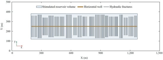
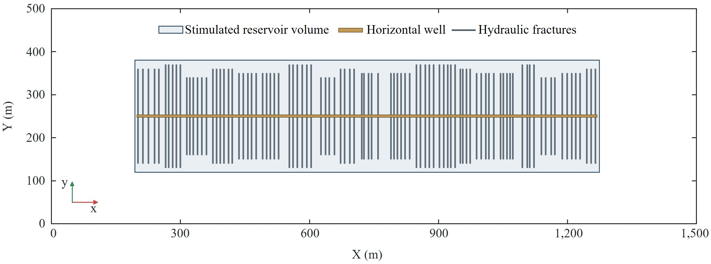
Equation (1) was evaluated with the orientations of the bedding-plane fractures and of the tectonic fractures associated with the east–west- and northeast-trending fault sets [7]. Individual hydraulic fractures were reconstructed from fracturing-treatment data and explicitly connected to the horizontal wellbore, and the gridblocks containing them were locally refined. The hydraulic fractures and surrounding stimulated matrix define the stimulated zone, whereas all remaining reservoir gridblocks constitute the unstimulated reservoir. The areal grid and hydraulic-fracture geometry are shown in Figure 2, and the principal model parameters are listed in Table 1.

Figure 2. Plan view of the simulation grid and hydraulic-fracture layout for Well H2CHF.

Table 1. Principal parameters of the numerical model for Well H2CHF.

Parameter	Unit	Value
Grid dimensions	-	213 × 21 × 5
Model top depth	m	3000.0
Reservoir mid-depth	m	3015.0
Reservoir thickness	m	30.0
Rock compressibility	MPa−1	1.0 × 10−4
Horizontal permeability	10−3 μm2	0.05
Vertical permeability	10−3 μm2	0.005
Porosity	%	6.2
Reservoir temperature	℃	130
Initial reservoir pressure	MPa	51.0
Bubblepoint pressure	MPa	15.086
Lateral length	m	1106.3
Number of fracturing stages	-	20
Number of hydraulic fractures	-	97
Number of clusters per stage	-	2–5
Fracture half-length	m	90–120

2.1.2. Fluid Properties

The reservoir temperature, initial reservoir pressure, and measured bubblepoint pressure for Well H2CHF are 130 °C, 51.0 MPa, and 15.416 MPa, respectively. The oil is therefore initially undersaturated; below the bubblepoint pressure, solution gas is liberated and oil, gas, and water flow simultaneously. Based on the compositional analysis, CO₂ was retained as a separate component, whereas the remaining oil and gas components were lumped into six pseudocomponents: N₂–C₂, C₃–C₆, C₇–C₁₃, C₁₄–C₂₀, C₂₁–C₂₇, and C₂₈–C₃₆ (Table 2).

Table 2. Fluid composition and thermodynamic parameters for Well H2CHF.

Component	Mole Fraction (%)	Molar Mass (g mol−1)	Critical Pressure (MPa)	Critical Temperature (K)	Acentric Factor
CO2	0.505	44.010	7.376	304.20	0.225
N2–C2H6	33.816	18.192	4.677	205.77	0.021
C3H8–C6	11.218	64.633	3.685	442.95	0.213
C7–C13	28.980	124.937	2.667	604.26	0.405
C14–C20	12.455	233.690	1.678	745.49	0.716
C21–C27	8.326	320.425	1.269	819.69	0.929
C28–C36	4.700	419.22	0.963	889.44	1.129

Phase-behavior calculations were performed using the Peng–Robinson equation of state [46], with critical temperature, critical pressure, acentric factor, and molar mass as input parameters. Hydrocarbon-phase viscosities were calculated using the HZYT correlation. Phase equilibrium was determined from the equality of component fugacities in the oil and gas phases, and CMG-GEM used this fluid model to calculate phase densities, viscosities, formation volume factors, and compositions during the simulation. The calculated bubblepoint pressure (15.086 MPa), oil density, viscosity, oil formation volume factor, and solution gas–oil ratio agree with the PVT measurements of the Well H2CHF oil sample to within 5.21% (Table 3).

Table 3. Comparison of measured and calculated PVT properties of the Well H2CHF oil at 130 °C.

Property	Condition	Measured	Calculated	Relative Difference (%)
Bubblepoint pressure (MPa)	-	15.416	15.086	−2.14
Oil density (g·cm−3)	51.0 MPa	0.7539	0.7146	−5.21
Oil viscosity (mPa·s)	51.0 MPa	1.405	1.434	+2.07
Oil formation volume factor (m3·m−3)	51.0 MPa; flash to 20 °C, 0.101 MPa	1.2213	1.1748	−3.81
Solution gas–oil ratio (m3·m−3)	Flash to 20 °C, 0.101 MPa	67.41	64.30	−4.62

2.1.3. Multiphase Compositional-Flow Equations

The same component-conservation and phase-flow equations govern the three flow domains, which differ in porosity, absolute permeability, relative permeability, capillary pressure, and pressure sensitivity.

Under isothermal conditions, molar conservation for any component j is expressed as follows:

$$\frac{\partial }{\partial t}\left[{\varphi }_N{\displaystyle \sum _{\alpha =o,w,g}{S}_{\alpha }}{c}_{\alpha }{x}_{\mathit{j\alpha }}\right]+\nabla \cdot \left[{\displaystyle \sum _{\alpha =o,w,g}{c}_{\alpha }}{x}_{\mathit{j\alpha }}{v}_{\alpha }\right]=q_j,$$

(2)

Component fluxes are expressed in terms of phase flow, with the Darcy velocity of each phase given by the following:

$$v_{\alpha }=-\frac{K_N(p_N)k_{\mathit{r\alpha }}}{{\mu }_{\alpha }}\left(\nabla p_{\alpha }-{\rho }_{\alpha }g\nabla z\right),$$

(3)

The saturations and pressures of the three phases satisfy the following closure relations:

$$\left\{\begin{array}{l}{S}_o+S_w+S_g=1\\ p_o-p_w=p_{\mathit{cow}}(S_w)\\ p_g-p_o=p_{\mathit{cgo}}(S_g)\end{array}\right.,$$

(4)

2.1.4. Reservoir Elastic Response

Fracturing-fluid injection raises pore pressure and increases hydraulic-fracture aperture and pore volume. As pressure subsequently declines, the increase in effective stress causes pore-volume contraction and fracture closure, which reduce permeability and fracture conductivity.

For the matrix continuum and the equivalent natural-fracture continuum outside the refined fracture gridblocks, porosity varies linearly with pressure:

ϕ_N(p_N) = ϕ_N,0[1 + C_N(p_N − p₀)],

(5)

The value of C_N is listed in Table 1. Because permeability responds differently to pressure in the three flow domains, domain-specific pressure-sensitivity functions are applied:

K_N(p_N) = K_N,0F_K,N(p_N),

(6)

In the refined fracture gridblocks, Equation (5) is replaced by a compaction–dilation curve, and the porosity and permeability multipliers are interpolated along its pressure-increase or pressure-decrease branch according to the current fracture pressure:

$$\left\{\begin{array}{l}{\varphi }_h(p_h)={\varphi }_{h,0}{M}_{\varphi ,h}^b(p_h)\hfill \\ K_h(p_h)=K_{h,0}{M}_{K,h}^b(p_h)\hfill \end{array}\right.,$$

(7)

Above the bubblepoint pressure, undersaturated oil expands as pressure declines, and the relationship between oil compressibility and oil formation volume factor is given by the following:

$$\left\{\begin{array}{c}{c}_o=-{\displaystyle \frac{1}{B_o}}{\left({\displaystyle \frac{\partial B_o}{\partial p}}\right)}_T\\ B_o(p)=B_o(p_b)\exp \left[-c_o(p-p_b)\right]\end{array}\right.,$$

(8)

Once pressure falls below the bubblepoint pressure, the model calculates solution-gas liberation and the resulting changes in oil- and gas-phase compositions from the component-conservation equations and phase-equilibrium relations.

2.1.5. Representation of Oil Displacement by Fracturing-Fluid Imbibition

During injection, fracture pressure exceeds matrix pressure and drives fracturing fluid into the stimulated matrix. During shut-in, the fracture–matrix pressure difference diminishes, while capillary forces continue to draw water into the matrix and displace oil toward the fractures, from which the oil flows to the wellbore once production begins. The model represents this process through the oil–water capillary pressure and relative permeability of each flow domain:

$$\left\{\begin{array}{l}{p}_{\mathit{cow},N}=p_{o,N}-p_{w,N}=f_{\mathit{pc},N}(S_w)\\ k_{\mathit{rw},N}=f_{\mathit{rw},N}(S_w)\\ k_{\mathit{ro},N}=f_{\mathit{ro},N}(S_w)\end{array}\right.,$$

(9)

2.1.6. Initial Conditions and Numerical Solution

The model simulated fracturing-fluid injection, shut-in, and production as a continuous sequence starting from pre-fracturing reservoir conditions.

The initial reservoir conditions at the reference depth of 3000 m were specified as follows:

$$\left\{\begin{array}{l}{p}_0=51 \mathrm{MPa}\\ T=130 °\mathrm{C}\end{array}\right.,$$

(10)

The initial pressure at other depths was obtained from vertical equilibrium. A no-flow condition was imposed at the outer model boundary Γ_e:

$$\left\{\begin{array}{c}n\cdot v_{\alpha }=0\\ x\in {\Gamma }_e\end{array}\right.,$$

(11)

Because the outer boundary is closed, the wellbore is the only pathway through which fluid enters or leaves the model. Fracturing fluid was injected at a constant rate of 5000 m³/d for 20 d from 1 June 2022, and the well was then shut in for 20 d. During flowback and natural-flow production, a vertical-flow performance relationship coupled the bottomhole and wellhead pressures; during artificial lift, production was constrained to a fixed liquid rate. The pressure, saturation, and phase-composition fields at the end of each stage served as the initial conditions for the next stage.

2.1.7. History Matching

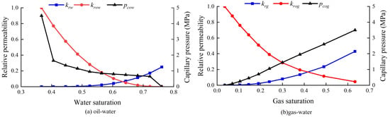
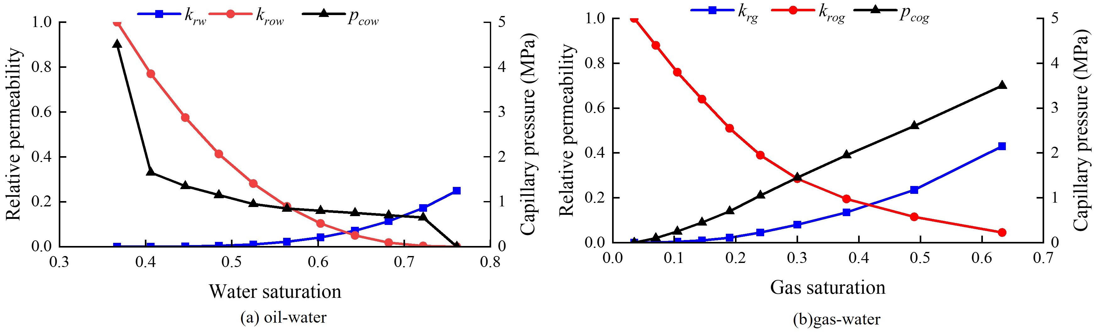
The daily oil rate, water cut, and bottomhole pressure of Well H2CHF from 11 July 2022 to 1 January 2024 were used as history-matching targets. The well trajectory, the locations of the fracturing stages and clusters, and the hydraulic-fracture geometry were held fixed. The measured daily liquid production rate was imposed as the well-rate constraint. History matching was performed manually. The equivalent matrix permeability (Section 2.1.1), the rock compressibility, and the compaction–dilation parameters of the hydraulic fractures (Section 2.1.4) were first adjusted to reproduce the bottomhole pressure. The oil–water relative permeability and capillary-pressure parameters were then adjusted to match the water cut, and the resulting daily oil rate was compared with the field data. The calibrated equivalent matrix permeability and rock compressibility are listed in Table 1. On the calibrated compaction–dilation curve, the porosity and permeability multipliers of the hydraulic fractures increase along the elastic branch from 0.85 and 0.1 at atmospheric pressure to 1.05 and 1.5 at 65 MPa; dilation above 65 MPa raises them to 1.20 and 10 at 66 MPa, and on subsequent unloading, they decrease to 0.90 and 0.2 at atmospheric pressure. The relative permeability and capillary pressure of the history-matched model are shown in Figure 3.

Figure 3. Relative permeability and capillary pressure of the history-matched model: (a) oil-water; (b) gas-oil.

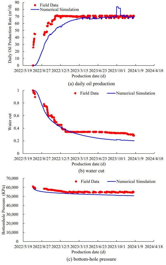
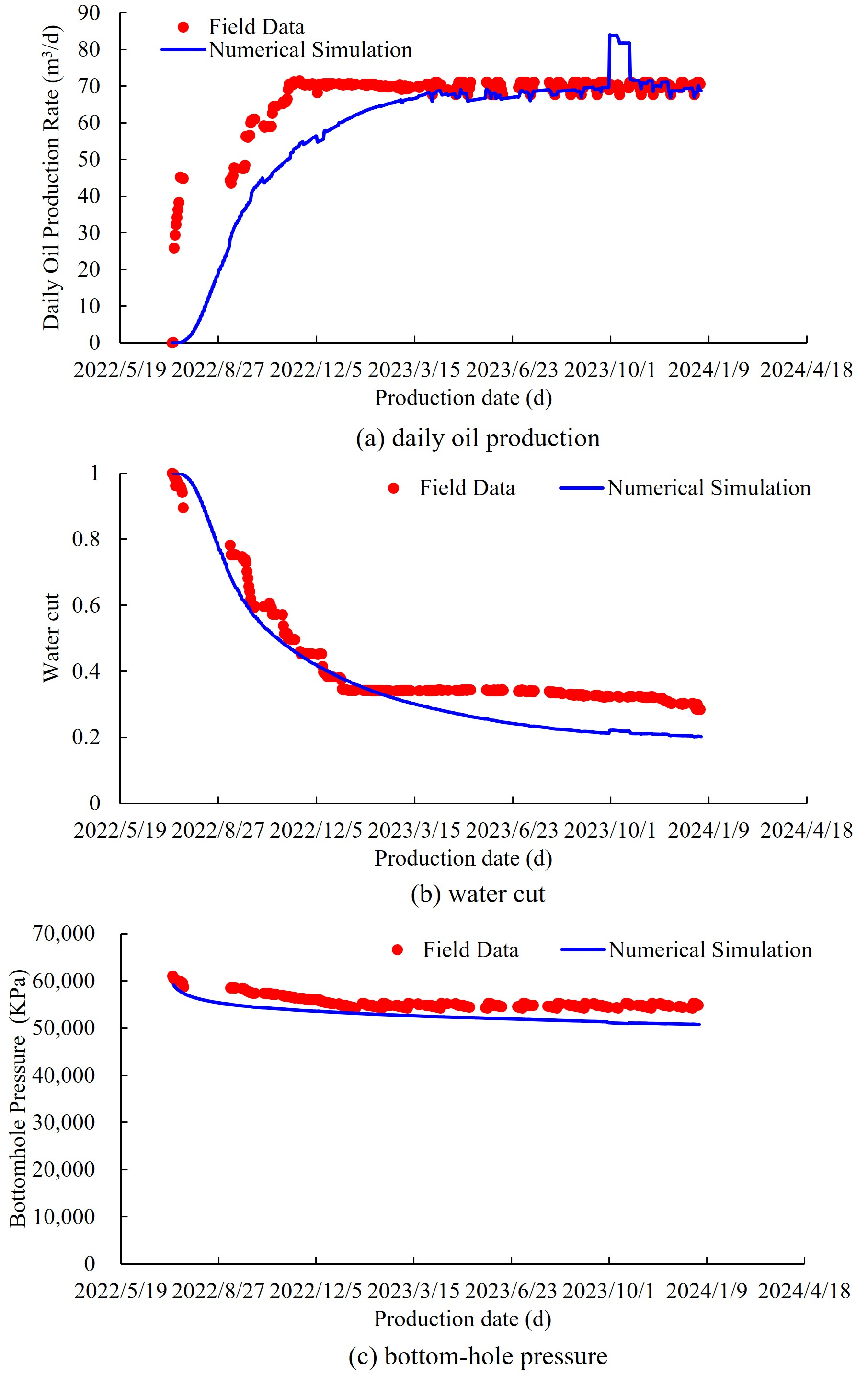
The mean absolute percentage errors (MAPEs) for daily oil rate and bottomhole pressure were 13.06% and 4.95%, respectively. The mean absolute error (MAE) in water cut was 6.74 percentage points, and the coefficient of determination (R²) for water cut was 0.723 (Figure 4). The oil-rate deviation was concentrated in the first three months of flowback, with a MAPE of 55.68%, compared with 8.57% for the subsequent production, and arose mainly in the first days after the well was opened, when the simulated production was still almost entirely fracturing fluid. Because the equivalent matrix permeability, rock compressibility, and compaction–dilation parameters were calibrated against the bottomhole pressure, which was reproduced in both periods (MAPEs of 4.80% and 4.96%), this deviation does not affect their calibrated values.

Figure 4. Production history match for Well H2CHF.

2.2. Oil Mobilization Across Control Regions

2.2.1. Net Oil Withdrawal by Control Region

During production, oil flows from the unstimulated reservoir through the stimulated matrix and hydraulic fractures into the wellbore. Because the same oil crosses several regional interfaces, cumulative interface flows would count it more than once; oil mobilization in each control region is therefore quantified by the net change in its oil inventory. Based on position along the oil-flow pathway, the reservoir is partitioned into three control regions: hydraulic fractures, represented by explicitly modeled fracture gridblocks; stimulated matrix, comprising the matrix gridblocks within the stimulated zone but excluding the fracture gridblocks; and unstimulated reservoir, comprising the reservoir gridblocks outside the stimulated zone.

Following Wang et al. [30], who evaluated oil mobilization from changes in in-place oil inventory, the oil inventory in control region i at time t, expressed at surface conditions, is given by the following:

$$N_i(t)={\displaystyle \sum _{k\in {\Omega }_i}\frac{{\varphi }_k(t)S_{o,k}(t)V_{b,k}}{B_{o,k}(t)}},$$

(12)

Over any time interval [t_a, t_b], the net oil withdrawal from control region i is given by the following:

N_p,i(t_a,t_b) = N_i(t_a) − N_i(t_b),

(13)

A positive N_p,i indicates net oil withdrawal from control region i, and a negative value indicates net oil inflow. Because N_i is expressed at surface conditions, it changes only when stock-tank oil enters or leaves control region i. Oil expansion and the liberation of solution gas below the bubblepoint pressure change the reservoir volume of the oil and B_o,k(t) together and therefore leave its stock-tank amount unchanged. The three control regions make up the entire model and its outer boundary is closed, so oil transferred between regions appears as a net withdrawal from one region and an equal net inflow to another, and the sum of the net oil withdrawals from the three control regions equals the cumulative oil production at the wellhead over the same time interval, except for the hydrocarbon components that dissolve in or are released from the aqueous phase.

2.2.2. Oil Production per Unit Pressure Decline

Because bottomhole pressure does not represent the pressure change within each control region, the average reservoir pressure of control region i is defined by weighting the gridblock pressure by bulk volume:

$${\overline{p}}_i(t)={\displaystyle \frac{{\displaystyle \sum _{k\in {\Omega }_i}{p}_k}(t)V_{b,k}}{{\displaystyle \sum _{k\in {\Omega }_i}{V}_{b,k}}}},$$

(14)

Equations (13) and (14) are combined to obtain the relationship between average reservoir pressure and net oil withdrawal for each control region. The absolute slope of the pressure-depletion segment of the resulting curve gives the amount of oil produced per unit pressure decline:

$$D_{p,i}=-{\displaystyle \frac{\mathrm{d}{N}_{p,i}(t_a,t)}{\mathrm{d}{\overline{p}}_i(t)}},$$

(15)

For an approximately linear segment, D_p,i is defined as the magnitude of the fitted-line slope. When the relationship curve exhibits a change in slope, D_p,i is evaluated separately for each linear segment.

2.2.3. Drive-Mechanism Decomposition

During production, declining pressure causes pore-volume contraction and oil expansion, the invading fracturing fluid displaces oil, and, below the bubblepoint pressure, liberated solution gas contributes to oil production; these processes correspond to four drive mechanisms. In Equation (12), the oil inventory of each gridblock is the product of ϕ_k, S_o,k, and 1/B_o,k. Changes in B_o,k reflect oil expansion and, below the bubblepoint pressure, the liberation of solution gas; changes in ϕ_k reflect pore-volume contraction; and changes in S_o,k reflect the displacement of oil by water and gas. The net oil withdrawal from control region i over the time interval [t_a, t_b] is therefore decomposed by changing these three factors in turn, and the resulting contributions sum exactly to N_p,i.

The contribution from changes in the oil formation volume factor is given by the following:

$$Q_{B,i}(t_a,t_b)+Q_{G,i}(t_a,t_b)={\displaystyle \sum _{k\in {\Omega }_i}{\varphi }_k}(t_a)S_{o,k}(t_a)V_{b,k}\left[{\displaystyle \frac{1}{B_{o,k}(t_a)}}-{\displaystyle \frac{1}{B_{o,k}(t_b)}}\right],$$

(16)

The contribution from pore-volume contraction is given by the following:

$$Q_{C,i}(t_a,t_b)={\displaystyle \sum _{k\in {\Omega }_i}\frac{S_{o,k}(t_a)}{B_{o,k}(t_b)}}\left[{\varphi }_k(t_a)-{\varphi }_k(t_b)\right]V_{b,k},$$

(17)

The contribution from oil displacement arises from the decrease in oil saturation. Because S_o,k = 1 − S_w,k − S_g,k, it is divided into displacement by water, Q_D,w,i, and displacement by gas, Q_D,g,i:

$$\left\{\begin{array}{l}{Q}_{D,i}(t_a,t_b)={\displaystyle \sum _{k\in {\Omega }_i}\frac{{\varphi }_k(t_b)}{B_{o,k}(t_b)}}\left[S_{o,k}(t_a)-S_{o,k}(t_b)\right]V_{b,k}=Q_{D,w,i}+Q_{D,g,i}\\ Q_{D,w,i}(t_a,t_b)={\displaystyle \sum _{k\in {\Omega }_i}\frac{{\varphi }_k(t_b)}{B_{o,k}(t_b)}}\left[S_{w,k}(t_b)-S_{w,k}(t_a)\right]V_{b,k}\\ Q_{D,g,i}(t_a,t_b)={\displaystyle \sum _{k\in {\Omega }_i}\frac{{\varphi }_k(t_b)}{B_{o,k}(t_b)}}\left[S_{g,k}(t_b)-S_{g,k}(t_a)\right]V_{b,k}\end{array}\right.$$

(18)

The term arising from changes in oil formation volume factor is partitioned according to gridblock pressure relative to the bubblepoint pressure. For p_k ≥ p_b, the term is attributed to oil expansion and denoted by Q_B,i; for p_k < p_b, it represents the shrinkage of oil caused by solution-gas liberation and is denoted by Q_G,i. The reservoir initially contains no free gas, so the increase in gas saturation results from solution gas liberated below the bubblepoint pressure, whereas the increase in water saturation results mainly from the invading fracturing fluid. Q_D,w,i therefore represents oil displacement by fracturing fluid; in the stimulated matrix, it results primarily from pressure-driven displacement and capillary imbibition, and in the unstimulated reservoir, it captures fluid redistribution between control regions. Gas liberation thus affects net oil withdrawal in two opposite ways: the oil shrinks, giving a negative Q_G,i, whereas the liberated gas displaces oil, giving a positive Q_D,g,i. The contribution of solution-gas drive is therefore Q_G,i + Q_D,g,i.

For each production stage, the contribution from each drive mechanism is obtained by summing the corresponding values over successive time intervals. The resulting contributions satisfy the following:

N_p,i = Q_B,i + Q_C,i + Q_D,w,i + (Q_G,i + Q_D,g,i),

(19)

For N_p,i > 0, the fractional contribution of drive mechanism m to the net oil withdrawal from control region i is given by the following:

$$R_{m,i}={\displaystyle \frac{Q_{m,i}}{N_{p,i}(t_a,t_b)}}\times 100\%.$$

(20)

3. Results and Discussion

3.1. Stage Delineation

A base-case model incorporating the history-matched reservoir properties (Table 1), relative permeability, and capillary pressure (Figure 3) for Well H2CHF was used to simulate 10 years of production. Its grid dimensions are 230 × 21 × 5, and its 1700 m lateral is completed with 20 fracturing stages of five clusters each, giving 100 hydraulic fractures with a half-length of 150 m. On the compaction–dilation curve of the refined fracture gridblocks, the porosity and permeability multipliers increase along the elastic branch from 0.8 at atmospheric pressure to 1 at 51 MPa; dilation raises them to 1.25 and 50 at 54 MPa, and on unloading, they decrease to 1.20 and 5 at 51 MPa and to 1 at atmospheric pressure. The injection and shut-in schedule follows Section 2.1.6. Production started on 11 July 2022 at a maximum liquid rate of 110 m³/d with a maximum drawdown of 3.0 MPa; once the wellhead pressure fell below 18.0 MPa, artificial lift was represented by a fixed liquid rate of 50 m³/d.

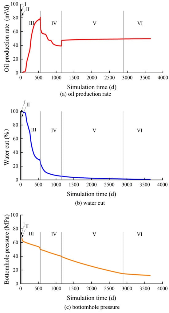
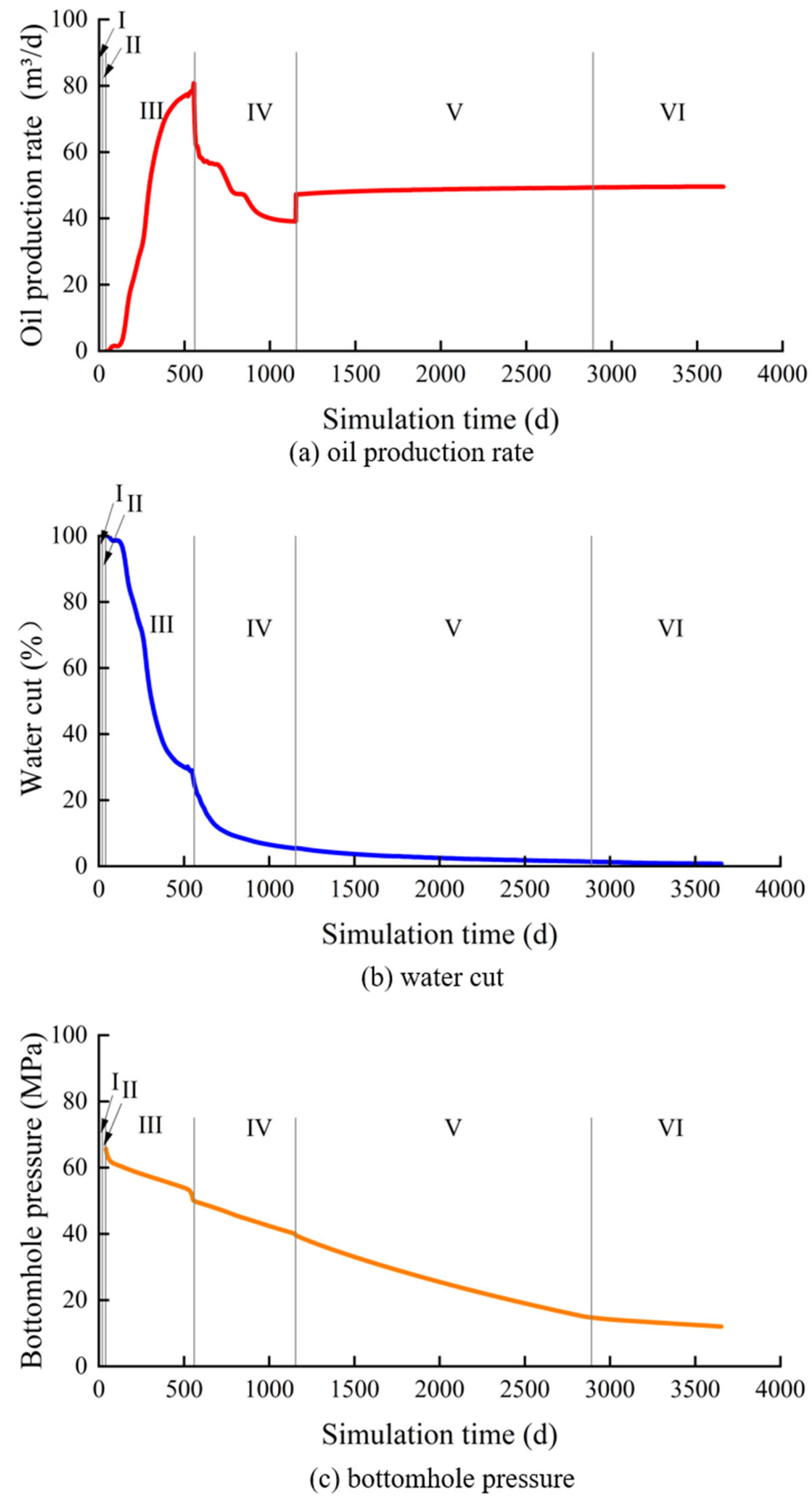
The production period after the well was opened was divided into stages based on daily oil rate, water cut, and bottomhole pressure. During flowback, water cut, initially 100%, declined rapidly, while daily oil rate reached a peak of 80.77 m³/d on day 554. After day 560, the well transitioned to declining production under natural flow. Artificial lift began on day 1155, after which, daily oil rate recovered from 39.10 to 47.27 m³/d and subsequently stabilized at 47.27–49.30 m³/d. On day 2891, bottomhole pressure fell to 14.77 MPa, below the bubblepoint pressure of 15.086 MPa, marking the onset of low-pressure production in the near-wellbore region. Accordingly, the complete sequence was divided into six stages: fracturing-fluid injection, shut-in imbibition, production buildup during flowback, natural-flow decline, stable production under artificial lift, and low-pressure depletion (Figure 5 and Table 4).

Figure 5. Dynamic responses and stage delineation of the base-case model throughout the fracturing–shut-in–production sequence. The intervals labeled I–VI denote fracturing-fluid injection, shut-in imbibition, production buildup during flowback, natural-flow decline, stable production under artificial lift, and low-pressure depletion, respectively. Vertical lines indicate the stage boundaries.

Table 4. Stage delineation for the base-case model.

Stage	Time (d)	Operating Mode	Dynamic Characteristics
Fracturing-fluid injection	0–20	Injection	Continuous fracturing-fluid injection; rapid pressure buildup in the hydraulic fractures and stimulated matrix
Shut-in imbibition	20–40	Shut-in	No wellhead production; redistribution of pressure and fluids between the hydraulic fractures and matrix
Production buildup during flowback	40–560	Open for flowback	Rapid decline in water cut; peak daily oil rate of 80.77 m3/d on day 554
Natural-flow decline	560–1155	Natural flow	Decline in daily oil rate to 39.10 m3/d; transition in production mode
Stable production under artificial lift	1155–2891	Artificial lift	Stable daily oil rate of 47.27–49.30 m3/d
Low-pressure depletion	2891–3653	Low-pressure production	Bottomhole pressure below the bubblepoint pressure; daily oil rate maintained at approximately 49 m3/d

3.2. Pressure Evolution and Oil Mobilization

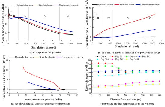
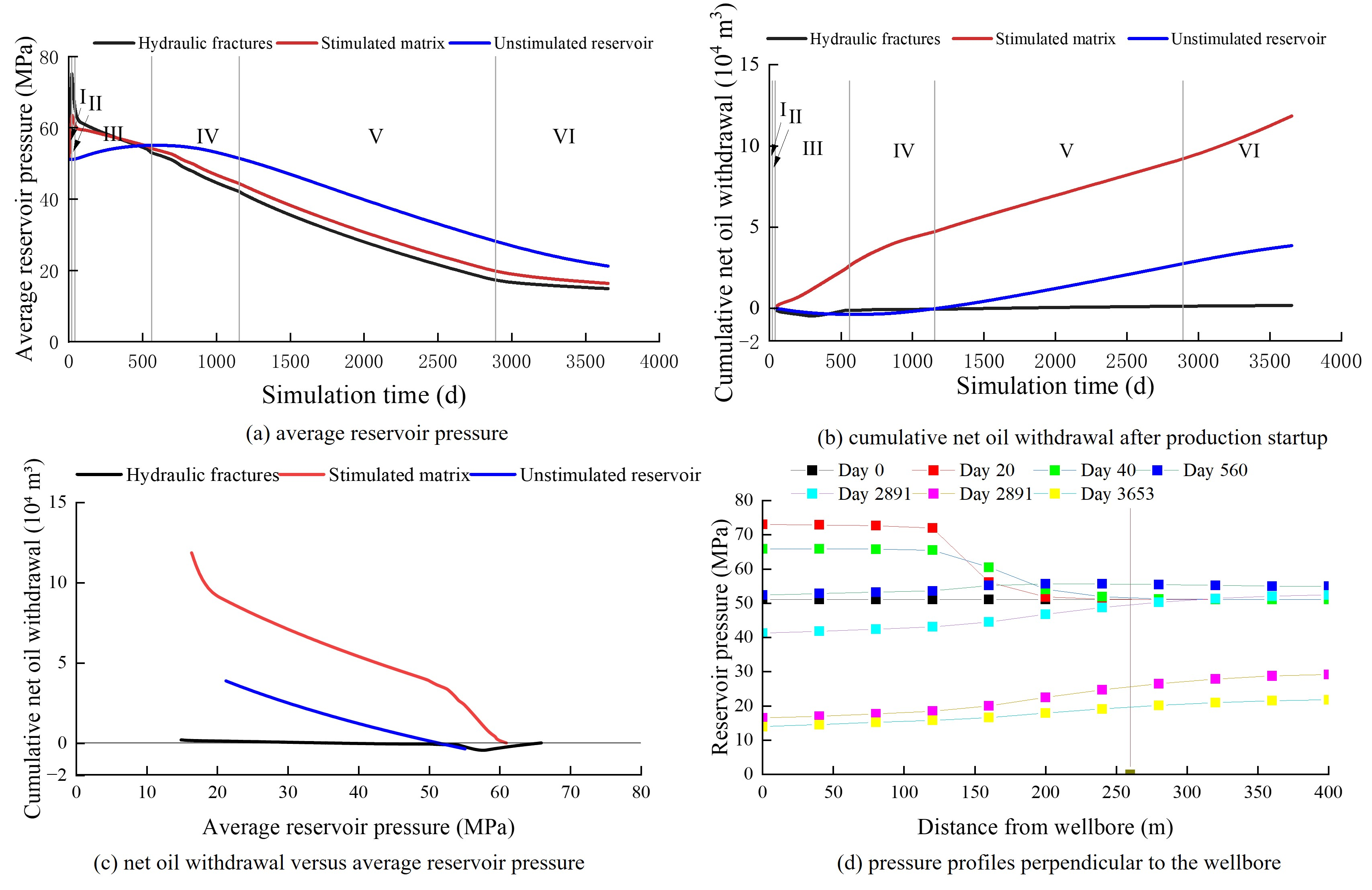
Figure 6a shows the successive propagation of fracturing-induced pressure buildup and production-induced pressure decline across the three control regions. During the 20 d of injection, the average pressures in the hydraulic fractures and stimulated matrix increased from the initial average of 51.11 MPa to 75.15 and 63.37 MPa (by 24.04 and 12.26 MPa), respectively, whereas that in the unstimulated reservoir increased by only 0.03 MPa. During the 20 d of shut-in, the former two fell to 65.92 and 60.95 MPa (by 9.23 and 2.42 MPa), while the unstimulated-reservoir pressure continued to rise to 51.26 MPa, indicating that the injection-induced pressure disturbance had begun to propagate outward. After production began on day 40, the hydraulic-fracture and stimulated-matrix pressures continued to decline, whereas the unstimulated-reservoir pressure continued to rise. The stimulated-matrix pressure exceeded the hydraulic-fracture pressure around day 328; around day 518, the unstimulated-reservoir pressure exceeded the stimulated-matrix pressure. These successive pressure crossovers established a stepwise pressure gradient from the unstimulated reservoir toward the wellbore. By the end of production, the average pressures in the hydraulic fractures, stimulated matrix, and unstimulated reservoir were 14.88, 16.37, and 21.23 MPa, respectively. The average hydraulic-fracture pressure had fallen below the bubblepoint pressure, whereas the unstimulated reservoir retained the highest pressure.

Figure 6. Pressure propagation and oil mobilization across the control regions: (a) average reservoir pressure; (b) cumulative net oil withdrawal after production startup; (c) net oil withdrawal versus average reservoir pressure; (d) pressure profiles perpendicular to the wellbore at the stage boundaries.

Figure 6d shows pressure profiles perpendicular to the wellbore at the stage boundaries; at each distance, pressure was averaged along the stimulated length of the lateral and weighted by gridblock bulk volume. At the end of injection, the pressure was 71.98–73.04 MPa within 120 m of the wellbore, where the hydraulic fractures are located, but only 51.85 MPa at 200 m. During shut-in, the pressure within 120 m fell by 6.47–7.10 MPa, whereas that at 160–280 m rose, showing outward propagation of the injection-induced pressure disturbance. On day 560, the pressure beyond 260 m, in the unstimulated reservoir, was 54.94–55.46 MPa and exceeded the 52.39–53.62 MPa within 120 m, consistent with the pressure crossovers in Figure 6a. From day 1155 onward, the pressure increased monotonically with distance from the wellbore; at the end of production, it ranged from 13.97 MPa at the wellbore to 21.81 MPa at 400 m.

During fracturing-fluid injection, net oil withdrawals from the hydraulic fractures and stimulated matrix were 0.441 × 10⁴ m³ and −0.137 × 10⁴ m³, respectively. During shut-in, the corresponding values were −0.302 × 10⁴ m³ and 0.378 × 10⁴ m³, respectively (Figure 6b). The sign reversals indicate that some of the oil that entered the stimulated matrix during injection flowed back during shut-in. The unstimulated reservoir showed a small net inflow during both stages, indicating that changes in oil inventory before production were largely confined to the region directly influenced by the hydraulic fractures. During production buildup in the flowback stage, net oil withdrawal from the stimulated matrix was 2.631 × 10⁴ m³, whereas those from the hydraulic fractures and unstimulated reservoir were −0.109 × 10⁴ m³ and −0.371 × 10⁴ m³, respectively. During natural-flow decline, net oil withdrawal from the unstimulated reservoir turned positive, reaching 0.355 × 10⁴ m³, although the oil accumulated through the preceding net inflow was not fully produced until day 1170. At the end of production, cumulative net oil withdrawals over the production period were 0.189 × 10⁴ m³, 11.853 × 10⁴ m³, and 3.864 × 10⁴ m³ for the hydraulic fractures, stimulated matrix, and unstimulated reservoir, respectively. These values represented 1.19%, 74.52%, and 24.29%, respectively, of the total net oil withdrawal (15.906 × 10⁴ m³). The hydraulic fractures therefore served mainly as flow pathways, whereas the stimulated matrix was the main source of oil. Oil supply from the unstimulated reservoir started later but stabilized after artificial lift began.

Figure 6c shows that the response of net oil withdrawal to pressure decline varied markedly with production stage among the three control regions. The hydraulic-fracture curve was relatively flat and shifted toward net inflow during early flowback. The stimulated-matrix curve exhibited a consistently negative slope immediately after production startup, with steeper segments during flowback and low-pressure depletion. The unstimulated-reservoir curve turned once the production-induced pressure decline reached the region, after which, net oil withdrawal increased approximately linearly with pressure decline (R² = 0.996–1.000). For the unstimulated reservoir, the magnitude of the curve slope increased progressively from stage to stage. The stimulated matrix consistently exhibited the highest oil production per unit pressure decline (Table 5).

Table 5. Oil production per unit pressure decline by control region and production stage (m³/MPa).

Production Stage	Hydraulic Fractures	Stimulated Matrix	Unstimulated Reservoir
Production buildup during flowback	—	4543.99	—
Natural-flow decline	51.52	1926.71	961.18
Stable production under artificial lift	76.64	1726.75	1137.59
Low-pressure depletion	213.49	7814.68	1596.16

The slope of the pressure–mobilization relationship during low-pressure depletion was used to extrapolate net oil withdrawal from each control region to a common limiting pressure:

$$N_{R,i}(p_{\lim })=N_{p,i}(t_0,t_e)+D_{p,i}^{\mathrm{L}}\max \left[{\overline{p}}_i(t_e)-p_{\lim },0\right].$$

(21)

By the end of the simulation, cumulative net oil withdrawal across the three control regions reached 15.906 × 10⁴ m³, corresponding to a recovery factor of 9.61%. When 15.086 MPa was adopted as the common limiting pressure, cumulative net oil withdrawal at the limiting pressure was projected to reach 17.894 × 10⁴ m³, raising the recovery factor to 10.81%. The stimulated matrix and unstimulated reservoir would contribute additional oil volumes of 1.007 × 10⁴ m³ and 0.981 × 10⁴ m³, respectively, whereas the contribution from the hydraulic fractures would be negligible. Although its remaining pressure was lower, the stimulated matrix would provide the larger increment because its oil production per unit pressure decline during low-pressure depletion was about five times that of the unstimulated reservoir.

3.3. Drive Mechanisms by Control Region

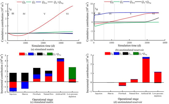
Net oil withdrawal was decomposed into the contributions of four mechanisms: oil expansion (Q_B), pore-volume contraction (Q_C), oil displacement by fracturing fluid (Q_D,w), and solution-gas drive (Q_G + Q_D,g). Figure 7 shows the cumulative changes in these contributions and their contributions in each stage. During fracturing-fluid injection, net oil withdrawal from the stimulated matrix was −0.137 × 10⁴ m³, while Q_B, Q_C, and Q_D,w were −1.176 × 10⁴ m³, −0.653 × 10⁴ m³, and 1.691 × 10⁴ m³, respectively. Injection-induced pressurization compressed the oil and expanded the pore volume, resulting in negative Q_B and Q_C values, whereas fracturing-fluid invasion reduced oil saturation and generated a positive Q_D,w. During shut-in, net oil withdrawal was 0.378 × 10⁴ m³; Q_D,w contributed 1.610 × 10⁴ m³ as the fracturing fluid continued to imbibe into the matrix, whereas Q_C was −1.320 × 10⁴ m³ because the pore volume continued to dilate as the pressure disturbance propagated into the matrix. During production buildup in the flowback stage, net oil withdrawal was 2.631 × 10⁴ m³, while Q_D,w, Q_C, and Q_B were 1.218 × 10⁴ m³, 0.840 × 10⁴ m³, and 0.573 × 10⁴ m³, respectively. Oil displacement by fracturing fluid and pore-volume contraction together supplied 78.23% of the net oil withdrawal in this stage and were the principal drive mechanisms.

Figure 7. Decomposition of net oil withdrawal by drive mechanism: (a,b) cumulative contributions in the stimulated matrix and unstimulated reservoir, respectively; (c,d) incremental contributions over the six operational stages in the corresponding regions.

During natural-flow decline, Q_B, Q_C, and Q_D,w accounted for 50.37%, 24.86%, and 24.78%, respectively, of net oil withdrawal from the stimulated matrix, whereas oil expansion dominated in the unstimulated reservoir, accounting for 88.77%. During stable production under artificial lift, the share of Q_B increased to 86.60% in the stimulated matrix and 94.59% in the unstimulated reservoir. During low-pressure depletion, net oil withdrawal from the stimulated matrix was 2.642 × 10⁴ m³. Displacement by liberated gas, Q_D,g, was 2.314 × 10⁴ m³, whereas Q_D,w was −0.129 × 10⁴ m³ because the retained fracturing fluid continued to flow back, and Q_G was −0.075 × 10⁴ m³ because the oil shrank as gas was liberated. Solution-gas drive, Q_G + Q_D,g, therefore contributed 2.239 × 10⁴ m³ (84.75%) and was the main drive mechanism in the stimulated matrix during this stage, followed by oil expansion (0.473 × 10⁴ m³, 17.91%).

Over the entire production period, oil expansion, pore-volume contraction, oil displacement by fracturing fluid, and solution-gas drive accounted for 50.49%, 15.60%, 14.75%, and 19.16%, respectively, of net oil withdrawal from the stimulated matrix. The corresponding shares in the unstimulated reservoir were 96.18%, 5.57%, −1.75%, and 0%, respectively. Across the two matrix regions, the four mechanisms contributed 61.73%, 13.13%, 10.69%, and 14.45%, respectively. Oil expansion was therefore the dominant mechanism in the matrix regions, and the other three mechanisms made comparable contributions.

Wang et al. [30] treated shut-in imbibition and displacement during production as one combined contribution, whereas the present study separates injection, shut-in, and production, so the contribution fractions of the two studies are not directly comparable. Both analyses nevertheless show that the dominant drive mechanism changes with time. Oil displacement by fracturing fluid was prominent from fracturing-fluid injection through production buildup in the flowback stage, during which, pore-volume contraction also contributed substantially. Oil expansion subsequently dominated during natural-flow decline and stable production under artificial lift, whereas solution-gas drive dominated during low-pressure depletion.

3.4. Sensitivity Analysis

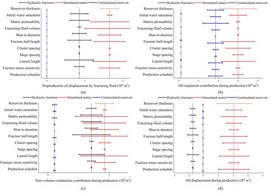
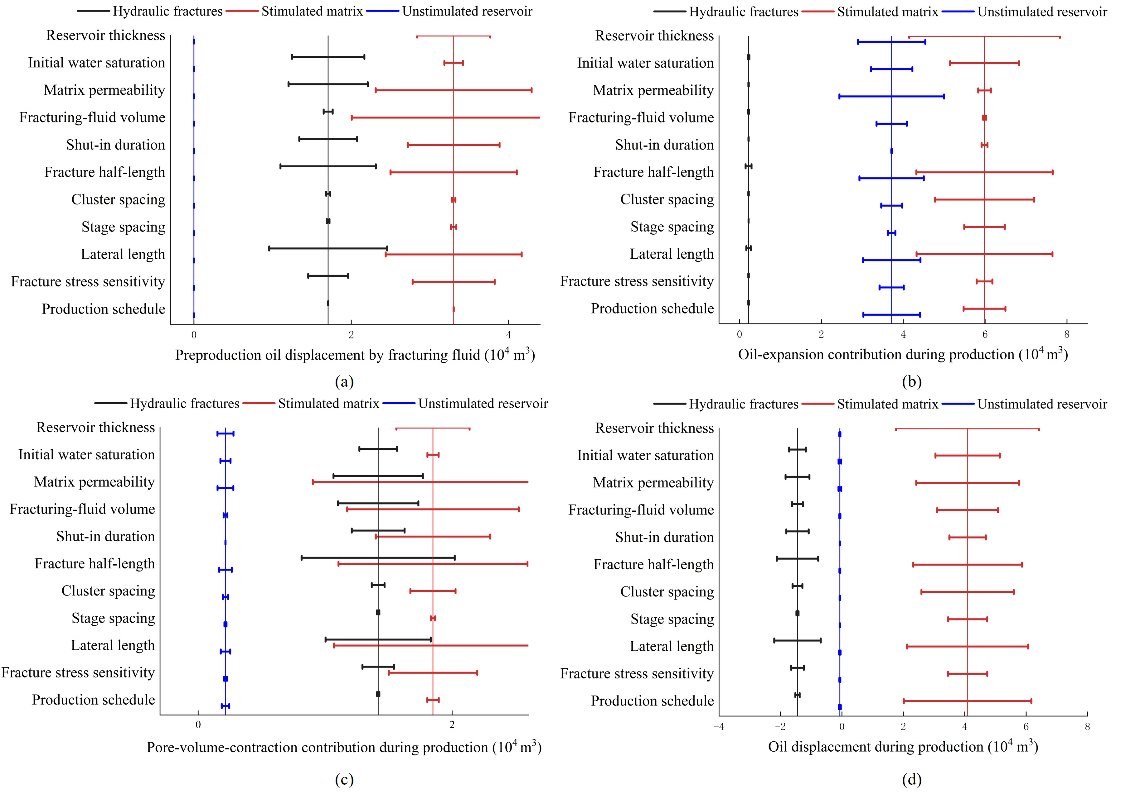
A total of 35 simulation cases were constructed from the base-case model by changing one factor at a time; the 11 factors cover reservoir properties, hydraulic-fracturing parameters, and production schedules (Table 6). In each case, the control regions were defined in the same way, and Equations (13)–(20) were used to calculate the regional responses. Figure 8 and Figure 9 summarize the calculated responses to the 11 factors. For each factor and control region, the horizontal bar spans the minimum and maximum values obtained from the base case and the cases in which that factor was varied over the values in Table 6, with all other inputs held at their base-case values; the dashed vertical lines indicate the base-case values.

Table 6. Settings of the sensitivity cases.

Factor	Base Case	Tested Values
Reservoir thickness (m)	30	20, 40, 50
Initial water saturation (%)	36.7	23.3, 30.0, 43.4
Matrix permeability (10−3 μm2)	0.05	0.01, 0.03, 0.07
Fracturing-fluid volume (104 m3)	10.0	6.0, 8.0, 12.0
Shut-in duration (d)	20	10, 30, 40
Fracture half-length (m)	150	100, 125, 175, 200
Cluster spacing (m)	15	9, 12, 18
Stage spacing (m)	25	20, 30, 35
Lateral length (m)	1700	1105, 1445, 1955
Fracture stress sensitivity	Base-case curve	L1, L2, L3
Production schedule (m3/d)	110/50	80/35, 95/43, 125/57, stepped

Note: spacing is center-to-center. Schedules are given as maximum/artificial-lift liquid rates; the stepped schedule raised the maximum rate from 50 to 105 m³/d. L1 and L2 dilate to porosity/permeability multipliers of 1.30/60 and 1.25/50 at 54 MPa and unload linearly; L3 starts dilating at 48 MPa.

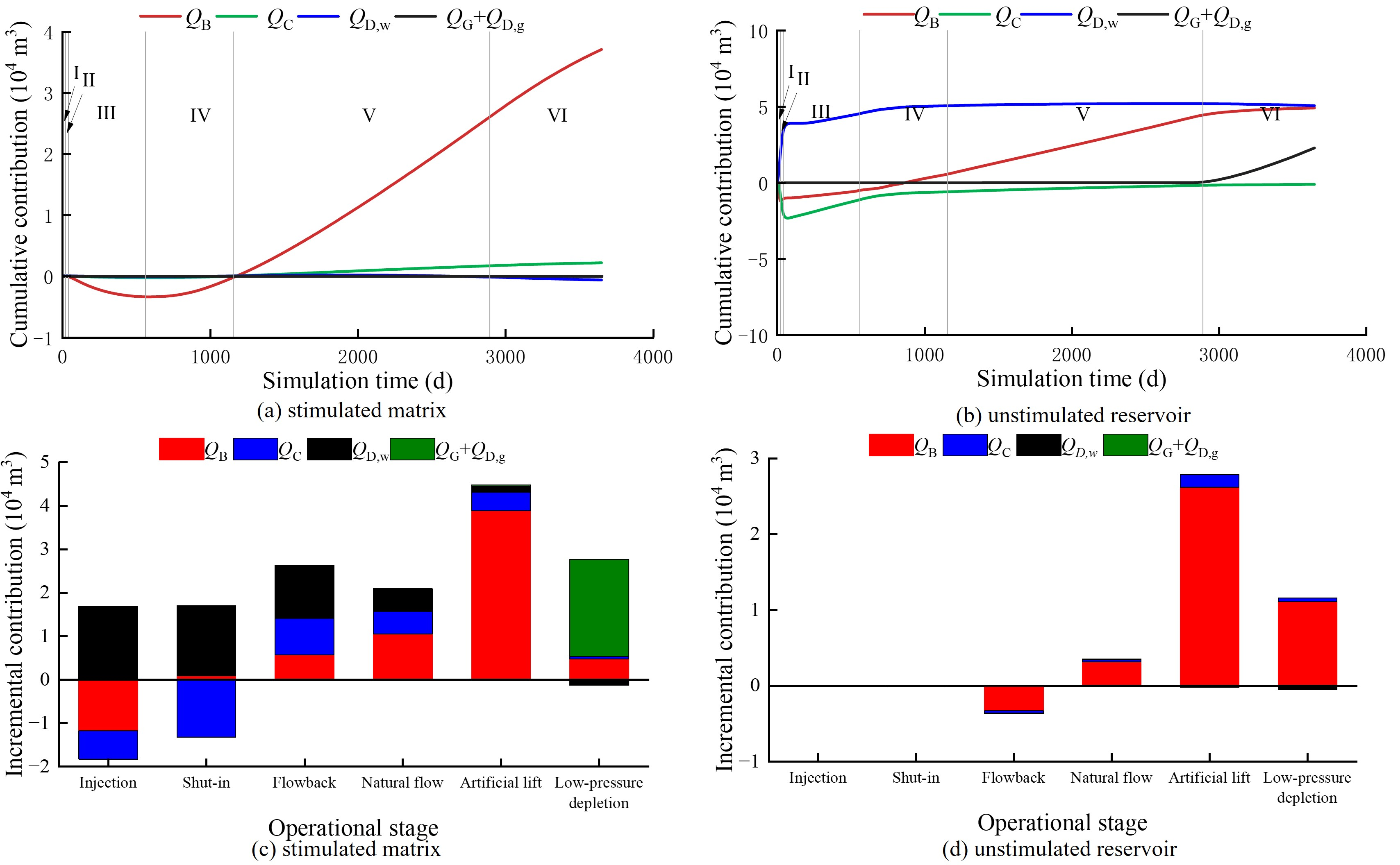
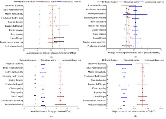
Figure 8. Effects of the 11 investigated factors on pressure and oil mobilization across the three control regions: (a) average reservoir pressure at production startup; (b) average reservoir pressure at the end of production; (c) net oil withdrawal during production; (d) net oil withdrawal per unit decline in average pressure during production. Bars show the range for each factor; dashed lines show the base case.

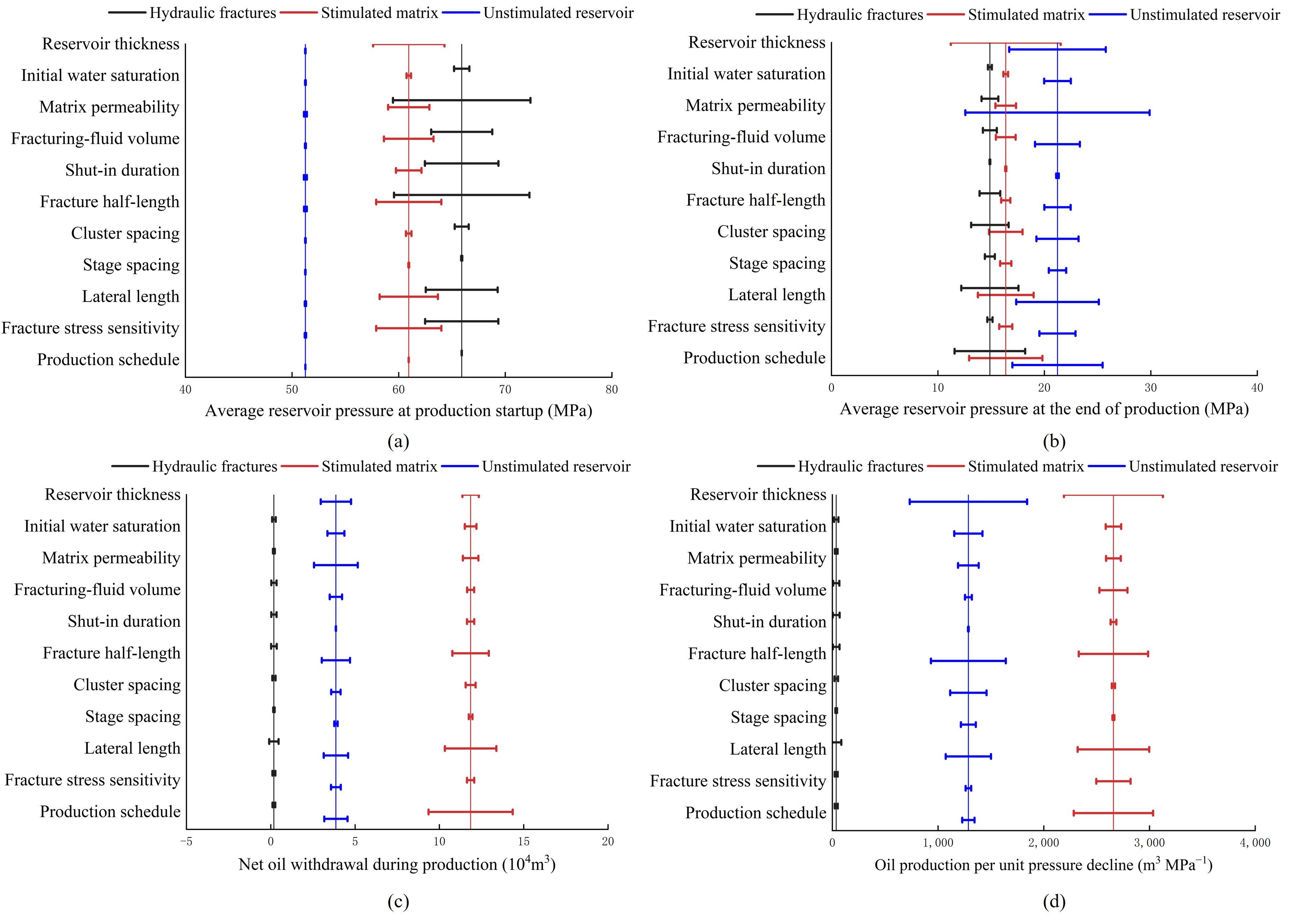
Figure 9. Effects of the 11 investigated factors on drive-mechanism contributions to net oil withdrawal across the three control regions: (a) preproduction oil displacement by fracturing fluid; (b) oil-expansion contribution during production; (c) pore-volume-contraction contribution during production; (d) oil displacement during production. Bars show the range for each factor; dashed lines show the base case.

3.4.1. Pressure Responses

Figure 8 shows the effects of the factors on regional pressure and oil mobilization. At production startup, differences among the simulation cases were almost entirely confined to the hydraulic fractures and stimulated matrix. The average pressure in the unstimulated reservoir varied by less than 0.4 MPa among the cases, indicating that the extent of fracturing-induced pressure buildup was constrained by the fracture-controlled reservoir volume. By the end of production, however, pressures in the unstimulated reservoir had diverged appreciably among the cases, reflecting differences in the extent to which production-induced pressure decline propagated outward. Net oil withdrawal from the hydraulic fractures remained close to zero, with both positive and negative values, so the fractures acted mainly as flow pathways. Consequently, the identification of primary controls focused on pressure decline and net oil withdrawal in the two matrix regions.

Table 7 summarizes the main controls and their quantitative effects. Reservoir thickness controlled the volume of oil mobilized per unit pressure decline: increasing thickness reduced the pressure buildup achieved by production startup but increased both the remaining pressure at the end of production and oil production per unit pressure decline. Consequently, total net oil withdrawal did not increase in direct proportion to reservoir thickness. Propagation of production-induced pressure decline beyond the stimulated matrix was governed primarily by matrix permeability and the degree to which fracture conductivity was retained. Higher matrix permeability shifted oil supply from the near-fracture–matrix toward the unstimulated reservoir, whereas greater fracture stress sensitivity limited the propagation of near-wellbore drawdown into the matrix. Fracturing-fluid volume and fracture-controlled reservoir volume determined the pressure and fluid distributions before production startup, although greater near-fracture pressure buildup did not translate proportionally into higher oil production per unit pressure decline. The production schedule did not affect reservoir conditions at production startup but directly controlled the magnitude of pressure depletion during production and therefore exerted the strongest operational control on net oil withdrawal. Initial water saturation and shut-in duration primarily affected fluid redistribution before production startup and had only a limited effect on total net oil withdrawal during production.

Table 7. Primary controls on pressure propagation and oil mobilization across the control regions.

Control Category	Primary Control and Investigated Range	Quantitative Response
Reservoir volume	Reservoir thickness: 20 → 50 m	Stimulated-matrix Dp,i: 2.41 × 103 → 3.35 × 103 m3/MPa; unstimulated-reservoir Dp,i: 0.88 × 103 → 1.99 × 103 m3/MPa
Pressure propagation	Matrix permeability: 0.01 → 0.07 10−3 μm2	Unstimulated-reservoir Np,i: 1.60 × 104 → 4.19 × 104 m3; stimulated-matrix Np,i: 12.77 × 104 → 11.85 × 104 m3
	Fracture stress sensitivity: L1 → L3	Stimulated-matrix Dp,i: 2.74 × 103 → 2.41 × 103 m3/MPa
Stimulation intensity	Fracturing-fluid volume: 6.0 × 104 → 12.0 × 104 m3	Stimulated-matrix preproduction QD,w,i: 1.55 × 104 → 4.14 × 104 m3
Production drawdown	Production schedule: 80/35 → 125/57 m3/d	Total Np,i: 11.66 × 104 → 18.19 × 104 m3
Secondary factors	Initial water saturation and shut-in duration	Limited variation among the simulation cases

3.4.2. Drive-Mechanism Responses

The investigated factors changed the magnitudes of individual drive-mechanism contributions but did not alter the basic roles of the three control regions (Figure 9). Across all simulation cases, oil supply from the unstimulated reservoir was consistently dominated by oil expansion. In the hydraulic fractures, the individual drive-mechanism contributions largely offset one another, leaving net oil withdrawal close to zero. Changes in drive composition therefore occurred mainly in the stimulated matrix.

Within the stimulated matrix, the drive balance shifted among oil displacement, pore-volume contraction, and oil expansion. Increasing fracturing-fluid volume or reducing the fracture-controlled reservoir volume increased the amount of fracturing fluid available per unit controlled volume, thereby strengthening oil displacement by fracturing fluid before production startup. By production startup, however, most of the displacement associated with the additional fracturing fluid had already occurred. Consequently, during production, the additional fracturing fluid increased the contribution from pore-volume contraction but reduced that from oil displacement, and net oil withdrawal from the stimulated matrix did not increase. Increasing reservoir thickness or matrix permeability expanded the reservoir volume over which oil expansion contributed to net oil withdrawal. A more aggressive drawdown schedule increased net oil withdrawal primarily by further reducing oil saturation in the stimulated matrix, with oil displacement providing the largest incremental contribution. Except for solution-gas drive, which operated only in cases in which the stimulated-matrix pressure fell below the bubblepoint pressure, the investigated factors did not change which drive mechanisms operated in each region. Instead, they altered the pressure trajectory and thereby changed the relative contributions of the existing mechanisms.

3.4.3. Primary Controls

Based on these responses, the investigated factors were classified into four categories of controls (Table 7): reservoir thickness as the reservoir-volume control; matrix permeability and fracture stress sensitivity as pressure-propagation controls; fracturing-fluid volume and fracture-controlled reservoir volume as stimulation-intensity controls; and the production schedule as the production-drawdown control. Fracture half-length, lateral length, and cluster and stage spacing acted indirectly by altering the fracture-controlled reservoir volume. Initial water saturation and shut-in duration had secondary effects.

3.5. Comparison with Other Shale Plays

Field and simulation studies from other basins report behavior consistent with the present results. In the Horn River Basin, wells with more complex fracture networks recovered less of the injected fracturing water during flowback [47]. In the present model, water production over 10 years amounted to 40.4% of the injected fracturing-fluid volume, and oil displacement by fracturing fluid in the stimulated matrix remained positive during injection and shut-in, indicating that most of the fracturing fluid was retained in the reservoir. In the Bakken, more intensive fracturing increased initial oil rates but steepened the subsequent decline [9]; here, increasing the fracturing-fluid volume from 6.0 × 10⁴ to 12.0 × 10⁴ m³ strengthened preproduction oil displacement but did not increase net oil withdrawal from the stimulated matrix during production (Section 3.4.2). For parent and child wells in the Eagle Ford, the DRV remained small and lagged behind the depth of investigation even after 30 years of simulated production [32], and in the Wolfcamp Formation of the Midland Basin, the extent of the DRV was controlled more by the enhanced permeability of natural fractures than by their storativity [48]. These observations are consistent with the delayed pressure decline in the unstimulated reservoir, the 74.52% share of the stimulated matrix in net oil withdrawal, and the control of matrix permeability on outward pressure propagation found here. In the west Eagle Ford, critical gas saturation strengthened solution-gas drive and reduced production decline [49]; in the present model, solution-gas drive became the main drive mechanism in the stimulated matrix once its pressure fell below the bubblepoint pressure. At the core scale, NMR measurements on Jimsar shale distinguished the effects of pore size and lithology on fracturing-fluid imbibition and damage [50], which are not resolved by the gridblock-scale oil displacement by fracturing fluid in the present model.

4. Conclusions

A history-matched compositional model of Well H2CHF was used to simulate the complete fracturing–shut-in–production sequence, and pressure, net oil withdrawal, and drive-mechanism contributions were quantified in the hydraulic fractures, stimulated matrix, and unstimulated reservoir. The main conclusions are as follows.

(1)

Fracturing-fluid injection increased the average pressures in the hydraulic fractures and stimulated matrix from 51.11 MPa to 75.15 and 63.37 MPa, respectively, while the pressure in the unstimulated reservoir remained nearly unchanged; the pressure disturbance then propagated outward. By the end of production, the average pressures in the three regions had declined to 14.88, 16.37, and 21.23 MPa, respectively, establishing a stepwise pressure gradient from the unstimulated reservoir toward the wellbore.

(2)

During the production period, the stimulated matrix accounted for 74.52% of the total net oil withdrawal and exhibited the highest oil production per unit pressure decline, whereas the hydraulic fractures served mainly as flow pathways. The recovery factor was 9.61% at the end of the simulation and increased to 10.81% when production was extrapolated to a limiting pressure of 15.086 MPa, corresponding to the bubblepoint pressure.

(3)

Oil expansion was the dominant drive mechanism, accounting for 61.73% of the combined net oil withdrawal from the two matrix regions, followed by solution-gas drive (14.45%), pore-volume contraction (13.13%), and oil displacement by fracturing fluid (10.69%). Oil displacement by fracturing fluid was prominent from fracturing-fluid injection through production buildup in the flowback stage, oil expansion dominated during natural-flow decline and artificial lift, and solution-gas drive dominated the net oil withdrawal from the stimulated matrix during low-pressure depletion.

(4)

The primary controls on oil mobilization across the control regions were reservoir thickness, matrix permeability and fracture stress sensitivity, fracturing-fluid volume and fracture-controlled reservoir volume, and the production schedule. These factors governed oil production per unit pressure decline, outward pressure propagation, preproduction pressure and fluid distributions, and pressure depletion during production, respectively. Initial water saturation and shut-in duration had comparatively limited effects.

The results are subject to several limitations. They were obtained from a single history-matched well model, and the regional shares depend on the extent assigned to the stimulated matrix, which was defined from the hydraulic-fracture layout. The fluid model does not account for nanopore confinement, which may shift the onset of gas liberation and hence the contribution of solution-gas drive. The recovery factor at the limiting pressure assumes that oil production per unit pressure decline remains at its low-pressure-depletion value, and the one-factor-at-a-time sensitivity analysis does not capture interactions between factors. The quantitative results therefore apply to wells with fluid, fracture, and operating conditions similar to those of Well H2CHF.

References

- Zou, C.; Pan, S.; Jing, Z. Shale oil and gas revolution and its impact. Acta Pet. Sin. 2020, 41, 1–12. [Google Scholar] [CrossRef]
- Sun, L.; Liu, H.; Zhu, R. Ten noteworthy issues on shale oil revolution in China. Acta Pet. Sin. 2023, 44, 2007–2019. [Google Scholar] [CrossRef]
- Jin, Z.; Wang, G.; Liu, G. Research progress and key scientific issues of continental shale oil in China. Acta Pet. Sin. 2021, 42, 821–835. [Google Scholar] [CrossRef]
- Fan, J.; Zhang, C.; Chang, R. Dynamic laws and stable production technology of Qingcheng shale oil development in Ordos Basin. Acta Pet. Sin. 2025, 46, 726–742. [Google Scholar] [CrossRef]
- Wang, Y.; Liu, C.; Duan, H. Maturity thresholds for continental shale oil enrichment based on thermal simulation experiments: A case study of the second member of Funing Formation in Gaoyou Sag, Subei Basin. Pet. Geol. Exp. 2026, 48, 708–720. [Google Scholar] [CrossRef]
- Fu, Q.; Duan, H.; Chen, W. Reservoir characteristics and influencing factors of shale oil in second member of Funing Formation, Gaoyou Sag, Subei Basin. Pet. Reserv. Eval. Dev. 2026, 16, 583–596. [Google Scholar] [CrossRef]
- Yang, Y.; Liu, Z.; Wang, R. Prediction and application of shale oil fractures: A case study of second member of Funing Formation in Huazhuang area, Gaoyou Sag, Subei Basin. Pet. Reserv. Eval. Dev. 2026, 16, 800–806. [Google Scholar] [CrossRef]
- Duan, H.; Shen, T.; Sun, J. Experimental study of oil matrix and fracture flow capacity of shale oil in Subei Basin. Pet. Reserv. Eval. Dev. 2024, 14, 333–342. [Google Scholar] [CrossRef]
- Male, F.; Duncan, I.J. The paradox of increasing initial oil production but faster decline rates in fracking the Bakken Shale: Implications for long term productivity of tight oil plays. J. Pet. Sci. Eng. 2022, 208, 109406. [Google Scholar] [CrossRef] [Scilit]
- Wachtmeister, H.; Lund, L.; Aleklett, K.; Hook, M. Production decline curves of tight oil wells in Eagle Ford Shale. Nat. Resour. Res. 2017, 26, 365–377. [Google Scholar] [CrossRef] [Scilit]
- Li, W.; Frash, L.P.; Welch, N.J. Stress-dependent fracture permeability measurements and implications for shale gas production. Fuel 2021, 290, 119984. [Google Scholar] [CrossRef] [Scilit]
- Shaibu, R.; Guo, B.; Wortman, P.B.; Lee, J. Stress-sensitivity of fracture conductivity of Tuscaloosa Marine Shale cores. J. Pet. Sci. Eng. 2022, 210, 110042. [Google Scholar] [CrossRef] [Scilit]
- Song, Z.; Song, Y.; Guo, J. Effect of nanopore confinement on fluid phase behavior and production performance in shale oil reservoir. Ind. Eng. Chem. Res. 2021, 60, 1463–1472. [Google Scholar] [CrossRef] [Scilit]
- Feng, D.; Lei, Z.; Wu, K. Phase behavior and composition distribution of shale oil in nanopore-bulk multiscale systems. Fuel 2025, 402, 136037. [Google Scholar] [CrossRef] [Scilit]
- Ren, Y.; Fan, J.; Xiao, Z. A coupled multi-mechanism modeling study for the fractured horizontal well in shale oil reservoirs. Energies 2026, 19, 1376. [Google Scholar] [CrossRef] [Scilit]
- Du, M.; Yang, Z.; Lyu, W. Experiment of dynamic seepage of tight/shale oil under matrix fracture coupling. Pet. Explor. Dev. 2024, 51, 356–366. [Google Scholar] [CrossRef]
- Zhang, S.; Sun, H.; Liu, Z. Research on flow mechanism and development law of Jiyang shale oil. Pet. Geol. Recovery Effic. 2024, 31, 38–47. [Google Scholar] [CrossRef]
- Du, S.; Shen, W.; Zhao, Y. Quantitative evaluation of stress sensitivity in shale reservoirs: Ideas and applications. Chin. J. Theor. Appl. Mech. 2022, 54, 2235–2247. [Google Scholar] [CrossRef]
- He, Y.; Huang, H.; Tang, M. Influence mechanisms of pressure difference in fracture ends on dynamic imbibition and displacement in shale reservoirs. J. China Univ. Pet. 2024, 48, 114–122. [Google Scholar] [CrossRef]
- Zuo, L.; Zhang, S.; Shen, Z. Mechanism of fracturing fluid imbibition in shale oil reservoirs. Acta Pet. Sin. 2024, 45, 1652–1661. [Google Scholar]
- Ouyang, W.; Zhang, M.; Sun, H. Numerical simulation of oil displacement by fracturing imbibition in horizontal shale oil wells. Pet. Drill. Tech. 2021, 49, 143–149. [Google Scholar] [CrossRef]
- Hu, Y.; Zhao, C.; Zhao, J. Mechanisms of fracturing fluid spontaneous imbibition behavior in shale reservoir: A review. J. Nat. Gas. Sci. Eng. 2020, 82, 103498. [Google Scholar] [CrossRef] [Scilit]
- Su, Y.; Sun, Q.; Wang, W. Spontaneous imbibition characteristics of shale oil reservoir under the influence of osmosis. Int. J. Coal Sci. Technol. 2022, 9, 69. [Google Scholar] [CrossRef] [Scilit]
- Zhu, J.; Wang, F.; Zhang, S.; Ma, X. Experimental research on behavior of spontaneous imbibition and displacement after fracturing in terrestrial shale oil based on nuclear magnetic resonance measurements. Processes 2024, 12, 2685. [Google Scholar] [CrossRef] [Scilit]
- Wang, Q.; Zhao, J.; Hu, Y. Shut-in time optimization after fracturing in shale oil reservoirs. Pet. Explor. Dev. 2022, 49, 586–596. [Google Scholar] [CrossRef]
- Liao, K.; Zhang, S.; Xie, B. Simulation of reasonable shut-in time for shale oil after volume fracturing. Pet. Reserv. Eval. Dev. 2024, 14, 749–755. [Google Scholar] [CrossRef]
- Wang, J.; Qu, Z.; Guo, T. Numerical simulation of post-fracturing flowback considering fracturing fluid imbibition. J. Shenzhen Univ. Sci. Eng. 2023, 40, 56–65. [Google Scholar] [CrossRef] [Scilit]
- Shaibu, R.; Guo, B. The dilemma of soaking a hydraulically fractured horizontal shale well prior to flowback: A decade literature review. J. Nat. Gas Sci. Eng. 2021, 94, 104084. [Google Scholar] [CrossRef] [Scilit]
- Jia, P.; Ke, X.; Niu, L. Investigation of shut-in effect on production performance in shale oil reservoirs with key mechanisms. Front. Earth Sci. 2022, 9, 782279. [Google Scholar] [CrossRef] [Scilit]
- Wang, F.; Qiao, R.; Li, J. Calculation of drained rock volume in shale oil reservoirs under the synergistic effect of imbibition and drainage displacement. Acta Pet. Sin. 2025, 46, 1157–1167. [Google Scholar] [CrossRef]
- Mayerhofer, M.J.; Lolon, E.P.; Warpinski, N.R. What is stimulated reservoir volume? SPE Prod. Oper. 2010, 25, 89–98. [Google Scholar] [CrossRef] [Scilit]
- Khanal, A.; Weijermars, R. Pressure depletion and drained rock volume near hydraulically fractured parent and child wells. J. Pet. Sci. Eng. 2019, 172, 607–626. [Google Scholar] [CrossRef] [Scilit]
- Xu, G.; Du, J.; Zhu, M. Practice and understanding of water huff-n-puff in shale oil of Subei Basin. Pet. Reserv. Eval. Dev. 2024, 14, 256–266. [Google Scholar] [CrossRef]
- Li, Y.; Zhu, Y.; Li, Z. Shale oil recovery by CO2 injection in Jiyang Depression, Bohai Bay Basin, East China. Pet. Explor. Dev. 2024, 51, 855–864. [Google Scholar] [CrossRef]
- Milad, M.; Junin, R.; Sidek, A. Huff-n-puff technology for enhanced oil recovery in shale/tight oil reservoirs: Progress, gaps, and perspectives. Energy Fuels 2021, 35, 17279–17333. [Google Scholar] [CrossRef] [Scilit]
- Zhu, C.F.; Guo, W.; Wang, Y.P. Experimental study of enhanced oil recovery by CO2 huff-n-puff in shales and tight sandstones with fractures. Pet. Sci. 2021, 18, 852–869. [Google Scholar] [CrossRef] [Scilit]
- Zheng, A.; Lu, W.; Zhang, R.; Sun, H. Numerical study on the enhanced oil recovery by CO2 huff-n-puff in shale volatile oil formations. Energies 2024, 17, 4881. [Google Scholar] [CrossRef] [Scilit]
- Wan, Y.; Jia, C.; Lv, W. Recovery mechanisms and formation influencing factors of miscible CO2 huff-n-puff processes in shale oil reservoirs: A systematic review. Adv. Geo-Energy Res. 2024, 11, 88–102. [Google Scholar] [CrossRef] [Scilit]
- Xu, N.; Chen, Z.; Xu, W. Prediction and evaluation method for development effect of shale oil storage volume fracturing. Pet. Reserv. Eval. Dev. 2024, 14, 741–748. [Google Scholar] [CrossRef]
- Hou, L.; Yu, Z.; Luo, X. Key geological factors controlling the estimated ultimate recovery of shale oil and gas: A case study of the Eagle Ford shale, Gulf Coast Basin, USA. Pet. Explor. Dev. 2021, 48, 654–665. [Google Scholar] [CrossRef]
- Wang, Y.; Zhou, F.; Su, H. Intelligent optimization method of fracturing parameters for shale oil reservoirs in Jimsar Sag, Junggar Basin, NW China. Pet. Explor. Dev. 2025, 52, 734–743. [Google Scholar] [CrossRef]
- Wang, Q.; Wang, Y.; Wang, R. Evolution law of stress induced by pressure depletion in fractured shale reservoirs: Implications for subsequent refracturing and infill well development. Petroleum 2025, 11, 71–83. [Google Scholar] [CrossRef] [Scilit]
- Li, P.; Liu, Z.; Duan, H. Controlling factors of shale oil enrichment in the Paleogene Funing Formation, Gaoyou Sag, Subei Basin, China. Energy Fuels 2024, 38, 18521–18532. [Google Scholar] [CrossRef] [Scilit]
- Jin, Z.-H.; Johnson, S.E.; Fan, Z.Q. Subcritical propagation and coalescence of oil-filled cracks: Getting the oil out of low-permeability source rocks. Geophys. Res. Lett. 2010, 37, L01305. [Google Scholar] [CrossRef] [Scilit]
- Oda, M. Permeability tensor for discontinuous rock masses. Geotechnique 1985, 35, 483–495. [Google Scholar] [CrossRef] [Scilit]
- Peng, D.Y.; Robinson, D.B. A new two-constant equation of state. Ind. Eng. Chem. Fundam. 1976, 15, 59–64. [Google Scholar] [CrossRef] [Scilit]
- Ghanbari, E.; Dehghanpour, H. The fate of fracturing water: A field and simulation study. Fuel 2016, 163, 282–294. [Google Scholar] [CrossRef] [Scilit]
- Nandlal, K.; Weijermars, R. Impact on drained rock volume (DRV) of storativity and enhanced permeability in naturally fractured reservoirs: Upscaled field case from Hydraulic Fracturing Test Site (HFTS), Wolfcamp Formation, Midland Basin, West Texas. Energies 2019, 12, 3852. [Google Scholar] [CrossRef] [Scilit]
- Gherabati, S.A.; Browning, J.; Male, F. The impact of pressure and fluid property variation on well performance of liquid-rich Eagle Ford shale. J. Nat. Gas Sci. Eng. 2016, 33, 1056–1068. [Google Scholar] [CrossRef] [Scilit]
- Bai, L.; Guo, H.; Jiang, Z. NMR analysis of imbibition and damage mechanisms of fracturing fluid in Jimsar shale oil reservoirs. Processes 2025, 13, 3875. [Google Scholar] [CrossRef] [Scilit]
Disclaimer/Publisher’s Note: The statements, opinions and data contained in all publications are solely those of the individual author(s) and contributor(s) and not of MDPI and/or the editor(s). MDPI and/or the editor(s) disclaim responsibility for any injury to people or property resulting from any ideas, methods, instructions or products referred to in the content. |
© 2026 by the authors. Licensee MDPI, Basel, Switzerland. This article is an open access article distributed under the terms and conditions of the Creative Commons Attribution (CC BY) license.