


Abstract
Regional disparity in total factor efficiency under renewable energy inputs (TFREE) constrains balanced green development amid the global energy transition. This study covers 256 prefecture-level cities in China (2005–2024). TFREE is measured using a meta-frontier dynamic SBM model. Disparity sources are decomposed along four spatial dimensions with the Dagum Gini coefficient. Predictive contributions are analyzed through an XGBoost–SHAP framework within a First Nature–Second Nature perspective. Results show: (1) TFREE disparity shifted from convergence to sustained divergence at the 2011 turning point, forming a persistent “hot South, cold North” pattern. (2) The share of net between-group disparity rose under all dimensions; under the North–South dimension, between-group disparity has exceeded within-group disparity since 2020, becoming the primary source. (3) Second Nature factors make larger predictive contributions than First Nature factors, but this difference narrows over time; annual mean temperature shows the largest increase in contribution. (4) All factors display nonlinear associations with TFREE: GDP shows an overall upward trend; human capital turns persistently negative beyond its transition point; annual mean temperature presents a sign-switching point around 10–15 °C. These findings suggest that differentiated policies may need to consider economic gaps between regional groups, local natural conditions, and nonlinear factor characteristics.
1. Introduction
A structural shift from fossil energy to renewable energy is reshaping the global energy system [1]. The costs of wind and photovoltaic power have fallen steadily. Renewable energy now accounts for a rising share of the global energy mix [2]. However, rapid capacity expansion has not brought proportionate gains in resource allocation efficiency. This mismatch manifests as uneven grid integration, redundant factor inputs, and systematic disparities in technological conversion efficiency. Renewable energy development therefore faces a fundamental challenge: moving from scale expansion to efficiency-driven growth [3]. Scale-based indicators such as installed capacity or electricity generation cannot, on their own, reveal the underlying causes of these inefficiencies. Total factor efficiency offers a more comprehensive perspective. This approach captures output growth beyond individual input contributions, as well as the combined effects of technological progress, factor allocation, and institutional conditions. Conventional applications, however, proxy energy input with fossil energy or total energy consumption. This practice conflates shifts in input structure with overall consumption trends [4,5]. Replacing such proxies with renewable energy consumption yields total factor efficiency under renewable energy inputs (TFREE). TFREE thus centers the evaluation on renewable energy and views the energy transition from an efficiency perspective. This measure provides a more targeted tool for assessing the quality of renewable energy integration.
The effect of renewable energy input on total factor efficiency is not spatially homogeneous. Differences in factor endowments and institutional conditions cause its direction and intensity to vary systematically across regions. Where infrastructure is well developed, and technology absorption capacity is strong, renewable energy achieves effective synergy with other production factors. Where infrastructure is weak, by contrast, grid integration bottlenecks emerge, and conversion efficiency declines as input scale expands. Such uneven efficiency patterns now pose a common challenge to the global energy transition [6]. As the world’s largest investor in renewable energy, China faces this tension most acutely. The dual carbon goals have accelerated the incorporation of renewable energy into the factor input structure. Rapid aggregate growth, however, has masked deep-seated regional divergences [7]. Resource-rich regions continue to scale up renewable installations, but limited industrial carrying capacity prevents proportionate gains in factor allocation efficiency. Technology-intensive regions face the reverse problem: they possess stronger integration capability but remain constrained by natural resource endowments. The resulting resource–technology mismatch produces pronounced spatial differentiation in TFREE [8]. Advancing a balanced energy transition therefore requires identifying how these disparities evolve, along which geographic divides they arise, and how they are associated with natural and socioeconomic conditions.
Existing research on energy-related total factor efficiency has advanced along three interconnected fronts—efficiency measurement, regional disparity characterization, and driving mechanism identification. In efficiency measurement, the multi-factor framework pioneered by Hu and Wang [9] progressively expanded the input side from capital and labor to include land, technology, and informatization inputs [10] and undesirable outputs such as carbon emissions and pollutant emissions [11]. Despite this increasingly comprehensive factor coverage, energy input has consistently been proxied by fossil energy or total energy consumption, rather than by renewable energy consumption alone [12,13]. In parallel, measurement methodology has evolved substantially: the SBM model addressed the limitations of early radial DEA models by incorporating slack variables in a non-radial manner [14]; the dynamic extension introduced carry-over variables to endow efficiency evaluation with intertemporal continuity [15]; the super-efficiency extension enabled differentiation among efficient frontier units [16]; and the meta-frontier framework provided a unified benchmark for cross-group efficiency comparison [17,18]. Among existing scales—cross-country comparisons [13], provincial panels [12], prefecture-level cities [7], counties [19], and enterprises [20]—provincial studies are the most abundant, while city-level analyses with renewable energy as the energy input remain scarce. In regional disparity characterization, analytical tools have evolved from the Theil index [21] to the Dagum Gini coefficient, which overcomes the non-overlapping subgroup assumption and has become the mainstream decomposition method for energy efficiency inequality [22,23]. Kernel density estimation and spatial autocorrelation analysis have deepened the understanding of distributional dynamics and spatial clustering [24], while emerging spatiotemporal hotspot analysis integrating the Getis–Ord Gi* statistic with the Mann–Kendall trend test has enabled the tracking of hot and cold spot evolution [25]. Nevertheless, most studies decompose disparity along a single spatial dimension (typically the East–Central–West division), leaving unclear along which geographic divides disparity mainly arises. In driving mechanism identification, the Tobit model [26] and spatial Durbin model [27] remain the dominant two-stage tools, complemented by the geographical detector for factor screening [28], enabling systematic investigation of how technological innovation, industrial structure, and environmental regulation shape total factor productivity [29,30,31]. These studies concentrate on socioeconomic determinants, whereas renewable energy generation and deployment also depend on natural conditions such as wind speed and temperature. Their linear or log-linear specifications also cannot capture nonlinear associations or interactions among factors. Ensemble learning algorithms—particularly XGBoost [32] combined with the SHAP interpretable framework [33]—have demonstrated superior capacity for nonlinear decomposition in adjacent fields such as carbon emission analysis [34,35], but have seldom been applied to TFREE.
Three gaps remain. Energy-related efficiency studies evaluate aggregate energy use, and how effectively renewable energy and other inputs are converted into economic output has rarely been assessed at the city level. Disparity decomposition relies mainly on a single regional division, so it remains unclear along which geographic divides TFREE disparity arises. Factor analysis focuses on socioeconomic determinants under linear specifications, and a factor’s association with efficiency levels does not by itself show its contribution to gaps between regional means. Taking 256 prefecture-level cities in China from 2005 to 2024 as the sample, this study addresses these gaps starting from the characteristics of renewable energy and contributes to the literature in three respects. First, at the city level, it evaluates how effectively renewable energy and other inputs are converted into economic output under environmental constraints, rather than the energy-saving potential of aggregate energy use. With renewable energy consumption as the energy input, TFREE is measured with a meta-frontier dynamic SBM model using provincial technology groups, as provinces differ in renewable resources and technology pathways. Second, it compares the sources of disparity across multiple regional divisions, as renewable energy development in China differs along several geographic divides at once. The Dagum Gini coefficient is applied under five groupings across four spatial dimensions—the four major regions, the North–South divide, the Hu Huanyong Line, and river basins—to examine whether the main source of disparity differs across divisions. Emerging spatiotemporal hotspot analysis complements this with the evolution of local clustering. Third, because renewable energy generation and deployment depend on natural conditions, it extends the First Nature–Second Nature framework to renewable energy efficiency, using XGBoost–SHAP to compare the predictive contributions of the two types of factors over time and identify their nonlinear associations with TFREE. The additivity of SHAP values further decomposes the mean TFREE gaps between regional groups into factor contributions, linking city-level prediction to the mean-level dimension of regional disparity.
2. Research Design
2.1. Study Area and Data Sources
This study uses cities at or above the prefecture level in China (hereafter, prefecture-level cities) as the basic spatial unit, covering 20 periods from 2005 to 2024. Cities are excluded from the sample under any of two conditions: administrative boundary adjustments during the study period that disrupt time-series continuity, or the systematic absence of city-level renewable energy and environmental statistics. These exclusions ensure panel balance and cross-period comparability in DEA efficiency estimation.
The final sample comprises 256 cities, representing 88% of Eastern, 93% of Central, 74% of Western, and 94% of Northeastern prefecture-level cities. Figure 1 shows their spatial distribution.
Figure 1.
Study area.
City-level socioeconomic and environmental data are compiled from the China City Statistical Yearbook, the China Fixed Asset Investment Statistical Yearbook, and individual city statistical yearbooks. City-level CO2 emissions are estimated using the IPCC [36] emission factor method based on fuel-type-specific fossil fuel consumption data recorded in the above sources. City-level end-use consumption of wind power, hydropower, and solar power is taken from the city-level energy consumption dataset of Yang et al. [37]. This dataset ends in 2021, and the same method extends the series to 2022–2024. Provincial consumption of each of the three sources is derived from power generation, renewable power generation, and inter-provincial electricity transfers. Sectoral GDP and resident population serve as the city-level allocation weights for production sectors and residential use, respectively. Wind speed data are obtained from the National Cryosphere Desert Data Center. Temperature data are calculated from daily station-level observations in the Global Surface Summary of the Day (GSOD) dataset. Interior missing values are filled by linear interpolation and those at the endpoints by extrapolation. To test the influence of imputation, the regional disparity analysis is repeated after excluding observations with interpolated or extrapolated values. The city ranking of mean TFREE (Spearman ρ ≥ 0.98) and the temporal trend of the Gini coefficient (r ≥ 0.99 with the baseline series) remain essentially unchanged, and the largest component of the Dagum decomposition remains largely consistent under all five dimensions.
2.2. Indicator System Construction
Input indicators cover five dimensions: capital, labor, energy, land, and information infrastructure. Capital input is represented by total fixed asset investment and the number of patent grants, which capture physical capital formation and technological innovation capacity, respectively. Total fixed asset investment also serves as a desirable carry-over variable in the dynamic SBM model, where it captures the intertemporal transmission of accumulated productive capital. The number of patent grants (including invention, utility model, and design patents) measures the accumulated technological knowledge stock of a city [38]. In this study, the output dimension is defined as economic output and environmental emissions. Patents therefore represent the technological foundation supporting productive activities and are incorporated as an input rather than an output. Labor input is measured by the number of employees in urban units. Covering on-post staff across all types of urban legal entities, this indicator reflects the scale of labor input in the formal economic sector. Energy input is the core of the indicator system design. Conventional total factor energy efficiency uses total or fossil energy consumption as the energy input and measures energy-saving potential. Under this setting, renewable energy is only a component of the energy aggregate, and its input performance cannot be identified separately. The energy transition also concerns whether renewable energy can effectively support economic output with a lower environmental cost than fossil energy. Accordingly, end-use consumption of wind power, hydropower, and solar power is used as the energy input, so that the energy dimension of the efficiency measure consists of renewable energy. Alongside economic output, undesirable outputs such as CO2 and SO2 emissions are included. These emissions arise mainly from fossil fuel combustion, and all else being equal, cities more dependent on fossil energy have higher emissions. Renewable energy is thus evaluated as the energy input, while fossil energy affects the efficiency score through the environmental cost of its emissions. Land input is measured by built-up area, which reflects the developed space actually used for productive activities. The count of broadband internet access ports captures information infrastructure input and reflects the level of urban digitalization. The above indicator system systematically characterizes the comprehensive input structure of cities across physical capital, human resources, clean energy, spatial resources, and digital infrastructure.
Regional gross domestic product (GDP) serves as the desirable output. As the most comprehensive aggregate indicator of regional economic performance, GDP captures the value added across all productive sectors and reflects the joint contribution of capital, labor, energy, and technological inputs. GDP has been widely employed as the standard desirable output in total factor productivity and energy efficiency studies [9,12]. This choice ensures cross-study comparability and provides a unified benchmark for efficiency evaluation across heterogeneous cities. Undesirable outputs are specified along two dimensions, air pollution and water pollution, with three selected indicators: CO2 emissions, SO2 emissions, and industrial wastewater discharge. CO2 emissions reflect the intensity of greenhouse gas emissions at the city level and serve as a core indicator for measuring carbon reduction performance. SO2 emissions capture acidic gas pollution generated by fossil fuel combustion and are closely related to energy structure transformation. Industrial wastewater discharge measures the environmental externalities of industrial activity on the water environment. Incorporating all three types of pollutants into the efficiency measurement framework avoids the bias that can arise when a single emission indicator stands in for total environmental costs. This approach provides a more comprehensive reflection of the overall environmental costs borne by each city in the process of output expansion [39]. Among the above indicators, fixed asset investment and GDP are deflated using the fixed asset investment price index and the GDP deflator, respectively, and converted to constant prices with 2005 as the base year. Table 1 presents the detailed definitions and units of all indicators. Table 2 reports the descriptive statistics of all input and output variables.
Table 1.
Indicator system for TFREE measurement.
Table 2.
Descriptive statistics of input and output variables.
2.3. Research Methods
2.3.1. Improved Meta-Frontier Dynamic SBM Model
Conventional DEA assumes that each period is independent, ignoring the transmission of input factors across adjacent periods. Tone and Tsutsui [15] introduced carry-over variables into the SBM framework [14] to construct the dynamic SBM model. Carry-over variables are classified into four types: desirable, undesirable, free, and fixed. Suppose there are n decision-making units (j = 1, 2, ⋯, n) over T periods (t = 1, 2, ⋯, T). Each unit has m inputs, s1 desirable outputs, and s2 undesirable outputs. Let α denote the type of carry-over variable. The inter-temporal carry-over variables satisfy the following continuity constraint:
where z denotes the value of the i-th type-α carry-over variable of the j-th decision-making unit in period t, and λ denotes the corresponding weight coefficient. Incorporating slack information from three dimensions—input redundancy, desirable output deficiency, and undesirable output excess—the non-oriented overall efficiency 𝛿* is defined as:
where ω denotes the period weight, input weight, and output weight, s− denotes the input slack, s+ denotes the desirable output slack, and sbad and sgood denote the slacks for undesirable output and desirable carry-over variables, respectively. x, y, b, and z represent the input value, desirable output value, undesirable output value, and carry-over variable value, respectively. The efficiency ρ* for each period is defined as:
Under this indicator specification, input redundancy, desirable output shortfall, and undesirable output excess all lower the efficiency score. Other things being equal, cities that use more renewable energy without correspondingly higher economic output receive lower scores. Given the same output and other inputs, cities with higher emissions, typically those more dependent on fossil energy, also receive lower scores. A high TFREE therefore indicates that, relative to other cities, all inputs, including renewable energy, are converted into economic output more effectively overall and at a lower environmental cost.
The above model assumes a common technology frontier. However, provinces differ significantly in renewable energy technology pathways and resource conditions. To address technological heterogeneity, this study introduces the meta-frontier framework. All decision-making units are divided into k groups by provincial affiliation (n = n1 + n2 + ⋯ + nk). A group frontier is constructed for each group, together with a common meta-frontier.
A variable return to scale (VRS) technology is assumed throughout, as imposed by the convexity constraint , to prevent scale effects from being conflated with technical inefficiency across cities of heterogeneous size. The model for solving the meta-frontier efficiency θ* is as follows:
This study treats 256 prefecture-level and above cities as decision-making units over 20 consecutive periods (2005–2024). Fixed asset investment links adjacent periods as a desirable carry-over variable, reflecting the continuity of capital accumulation. Following the standard formulation of Tone and Tsutsui [15], all periods receive equal weights. In China, provincial governments form the core administrative level for energy policy and renewable energy planning. Provinces also differ markedly in renewable resource endowments and development priorities. Accordingly, the 256 cities are divided into 30 technology groups by provincial affiliation. Each group corresponds to one province and comprises all of that province’s prefecture-level and above cities meeting the sample selection criteria. The median group contains 9 cities. A group frontier is constructed from the cities of a single province and represents best practice under that province’s conditions. The common meta-frontier envelops all group frontiers and draws on the full sample of 256 cities. TFREE is measured against the common meta-frontier. Consequently, all cities share the same reference set irrespective of group size, ensuring comparability across groups. The resulting score reflects the overall allocation efficiency of renewable energy and other production factors under environmental constraints. Higher values indicate a more favorable balance among renewable energy utilization, economic output, and pollution abatement. To assess the robustness of this scheme, the sample is reclassified into four regions (Eastern, Central, Western, and Northeastern China; Figure 1), each containing a substantially larger number of cities. The Kruskal–Wallis test reveals significant differences in TFREE across the four regions (H = 240.55, df = 3, p < 0.001). This result indicates that the regional heterogeneity underlying the provincial grouping persists under a coarser classification. Group-frontier efficiency is then re-estimated with the four regions as technology groups. Spearman rank correlation coefficients measure the agreement between city rankings under the provincial and four-region groupings. The two rankings are significantly and positively correlated in every year (ρ > 0.63, all p < 0.001). The relative efficiency positions of cities therefore remain consistent to a considerable degree across the two schemes. All models are solved using MaxDEA 7 software.
2.3.2. Dagum Gini Coefficient
To systematically characterize the level of regional disparities in TFREE and their source structure, this study adopts the Gini coefficient and its decomposition method proposed by Dagum [22]. Compared with the conventional Gini coefficient and the Theil index, this method allows overlapping distributions across subgroups. It strictly decomposes the overall disparity into three components: within-group disparity (Gw), net between-group disparity (Gnb), and transvariation density (Gt). The three components satisfy G = Gw + Gnb + Gt. Suppose all n cities are divided into k groups. The j-th group contains nj cities. yji and yhr denote the TFREE values of the i-th city in the j-th group and the r-th city in the h-th group, respectively. μ is the overall sample mean, and μj is the mean of the j-th group. The overall Gini coefficient G is defined as:
The formulas for the within-group disparity Gw, net between-group disparity Gnb, and transvariation density Gt are as follows:
where Gjj and Gjh denote the within-group Gini coefficient of the j-th group and the Gini coefficient between the j-th and h-th groups, respectively. pj = nj/n, sj = njμj/(nμ), j = 1, 2, …, k, with μ1 ≤ μ2 ≤ … ≤ μk. Djh = (djh − pjh)/(djh + pjh) represents the relative influence of TFREE between the j-th and h-th groups. djh and pjh denote the expected positive parts of yji − yhr and yhr − yji, respectively. The formulas are as follows:
where Fj and Fh denote the cumulative distribution functions of the j-th and h-th groups, respectively.
2.3.3. Emerging Spatiotemporal Hotspot Analysis Method
The Gini coefficient and its decomposition reveal the magnitude and composition of regional disparities in numerical terms. However, they do not address the spatial distribution characteristics or the evolutionary direction of these disparities. To identify the temporal evolutionary trend of the spatial agglomeration pattern of TFREE, this study employs the emerging spatiotemporal hotspot analysis method. This method first constructs a space-time cube based on spatial locations and time steps. At each time slice, the Getis–Ord statistic is used to test the significance of local agglomeration between each city and its neighbors. The statistic is defined as:
where xj is the TFREE attribute value of city j, wi,j is the spatial weight between cities i and j, n is the total number of cities, and and S are the global mean and standard deviation, respectively. A significantly positive value indicates that the city and its neighbors form a high-value agglomeration (hot spot). A significantly negative value indicates a low-value agglomeration (cold spot). After calculating the value for each city in each year, the Mann–Kendall trend test is applied to statistically assess the temporal sequence. Based on significance across time steps and the trend test, each city is classified into a pattern in Table 3.
Table 3.
Emerging spatiotemporal hot spot patterns.
2.3.4. XGBoost–SHAP Interpretable Machine Learning Model
This study employs the XGBoost model [32] to identify the key factors associated with TFREE. The algorithm is based on gradient boosting decision trees with a regularization term balancing predictive accuracy and generalization capacity. XGBoost fits nonlinear relationships well, but its decision process lacks interpretability. To quantify the direction and intensity of each factor’s predictive contribution to TFREE, this study applies the SHAP method [33]. SHAP is rooted in the Shapley value from cooperative game theory, fairly allocating each prediction’s deviation from the mean prediction among all features. The Shapley value φi of feature i is defined as:
where N is the set of all features, S is any subset that does not contain feature i, and f(S ∪ {i}) and f(S) are the model outputs with and without feature i, respectively. A positive Shapley value indicates that feature i makes a positive contribution to the prediction. A negative value indicates a negative contribution.
3. Spatiotemporal Evolution of Regional Disparities in China’s Total Factor Efficiency Under Renewable Energy Inputs
3.1. Dynamic Evolution
Regional disparities in China’s TFREE are measured at the city and provincial scales for 2005–2024, using the Dagum Gini coefficient (Figure 2). Provincial TFREE is the GDP-weighted average of city-level TFREE within each province. The two Gini coefficient series track each other closely. Both converge initially and then diverge, forming a phased evolutionary pattern with 2011 as the turning point. A Chow structural break test confirms the statistical significance of this turning point at both the city scale (F = 32.25, p < 0.01) and the provincial scale (F = 22.96, p < 0.01).
Figure 2.
Spatiotemporal evolution of regional disparities in TFREE.
From 2005 to 2011, the city-level Gini coefficient fell by 21.0%, and city efficiency levels converged. A structural reversal followed in 2011. The Gini coefficient then shifted to a sustained upward trajectory, and efficiency differences among cities widened. This divergence was not uniform but proceeded in distinct phases. Between 2011 and 2016, the rise was slow. The increase accelerated in 2017–2018 and then partially retreated, a short-term fluctuation against the broader trend. After 2019, the pace quickened further, and cities separated more sharply in their capacity to raise efficiency. A slight decline occurred in 2024, yet the overall widening has not been reversed.
Although the city-level Gini coefficient remains consistently below its provincial counterpart, it has more than doubled since 2011. This rise indicates that inter-city efficiency disparities have evolved from a low level into a pronounced divergence. The provincial-level Gini coefficient follows a trajectory highly synchronous with the city-level series, reflecting cross-scale consistency of the phased pattern identified above.
Figure 3 depicts the spatial distribution of TFREE at four cross-sectional time points. In 2005, spatial differentiation was weak, with broadly similar values across cities and no distinct regional clustering. By 2011, the overall pattern remained similar, though a few cities—particularly in northern China—showed slight increases in value. In 2018, spatial differentiation began to emerge in the opposite direction: northern cities declined while southern and southeastern coastal cities deepened, and a preliminary north–south contrast took shape. By 2024, this differentiation became more evident. Higher-value cities concentrated in the Yangtze River Delta, the Pearl River Delta, and southeastern coastal areas, while lower-value cities were mainly distributed in the Northeast and Northwest, forming a “high-southeast, low-northwest” spatial gradient.
Figure 3.
Spatial patterns of regional disparities in China’s TFREE.
3.2. Emerging Spatiotemporal Hotspot Analysis
Emerging spatiotemporal hotspot analysis classifies each city’s TFREE into hot spot and cold spot categories. Unlike static cross-sectional maps, this approach integrates continuous spatiotemporal information across the full sample period and traces the evolutionary trajectory of each city’s agglomeration status (Figure 4). TFREE exhibits a pronounced “hot south, cold north” spatial differentiation pattern. Both hot spots and cold spots are dominated by the consecutive and intensifying types. This indicates that the current spatial polarization is characterized by persistence rather than cyclical fluctuation.
Figure 4.
Emerging spatiotemporal hotspot analysis of TFREE.
Hot spot areas concentrate in southeastern coastal and central-southern regions. Cities along the Fujian–Zhejiang coast and in the Pearl River Delta are classified as consecutive or new hot spots. These cities generally possess mature industrial systems and dense innovation resources, and their high-efficiency agglomeration has strengthened in recent years. Central-southern cities have recently shifted to new hot spots, indicating that high-efficiency areas are expanding from the coast toward the interior. Sporadic hot spots in the southern hinterland suggest that localized efficiency improvements have emerged, though agglomeration effects have not yet stabilized.
Cold spots concentrate in the Northeast. Cities in Heilongjiang and Jilin are classified as consecutive or intensifying cold spots. These cities are generally dominated by heavy industry and rely on a fossil-fuel-oriented energy structure. Their low-efficiency status has not been alleviated but has instead deepened further. Some cities from North China to the Huang–Huai region show persistent or diminishing cold spots with milder intensity. Marginal improvement has appeared, yet these cities have not moved out of the cold spot range overall. Most western cities show no significant pattern, consistent with the sparse distribution of cities in this region.
Taken together, the sustained rise in the Gini coefficient after 2011, the progressive strengthening of the “hot south, cold north” pattern across cross-sectional maps, and the dominance of consecutive and intensifying categories in the hotspot analysis indicate that the current spatial polarization is not a short-term fluctuation. Rather, it is a persistent pattern that has deepened over time.
3.3. Decomposition of Regional Disparity Dynamics
The preceding analysis reveals the aggregate trend of TFREE regional disparities, but cannot determine whether divergence originates between or within regional groups. China’s renewable energy industry exhibits pronounced multidimensional differentiation: systematic differences in resource endowments and market capacity exist across the Hu Huanyong Line; the North and South diverge in energy structure compatibility; the four major regions carry cumulative effects of differentiated development strategies; both the Yangtze River Economic Belt (YREB) and the Yellow River Basin (YRB) operate under distinct river-basin governance frameworks. A single-dimension classification cannot capture this multi-layered pattern. Accordingly, this study examines between-group and within-group disparities across four spatial dimensions: four major regions, the North–South divide, the Hu Huanyong Line, and river basins.
3.3.1. Between-Group Disparity
The multidimensional decomposition results are shown in Figure 5. The Dagum Gini coefficients for all ten regional pairs exhibit a U-shaped trajectory, generally declining between 2005 and 2011 before shifting to an upward trend. By 2024, all values exceeded their initial levels. Cross-dimensional comparison reveals a clear intensity gradient. Under the Hu Huanyong Line dimension, the between-group disparity is the most pronounced, peaking at 0.123 in 2022, the highest across all dimensions and all regional pairs. Under the four major regions dimension, the Eastern–Northeastern disparity is the most salient, reaching 0.084 in 2024, while the Central–Western disparity has the lowest absolute value in 2024, consistent with the relatively similar TFREE levels observed in these two regions. Under the North–South dimension, the coefficient follows a highly similar trajectory to the Eastern–Northeastern pair, reaching 0.082 in 2024. Under the river basin dimension, an expanding trend is observed, but the absolute level has remained lower than that of the Hu Huanyong Line and North–South dimensions since 2017.
Figure 5.
Between-group disparities from multiple spatial perspectives.
3.3.2. Within-Group Disparity
Within-group disparity also exhibits an overall widening trend, but its extent varies across groups (Figure 6).
Figure 6.
Within-group disparities from multiple spatial perspectives.
Under the four major regions dimension, the Eastern region shows the largest increase, reaching 0.084 in 2024, a pattern likely associated with the concentration of innovation resources in core cities. Disparity in the Western region has generally risen since 2013, peaking at 0.076 in 2022, possibly owing to efficiency leaps in a small number of cities with outstanding renewable energy endowments. The Central region has the lowest within-group disparity in most years. The Northeastern region experienced early convergence followed by a rebound after 2016, although its 2024 level remains close to that of 2005. Under the North–South dimension, within-group disparity in the northern group has increased markedly since 2020, whereas the southern group has remained largely stable. Under the Hu Huanyong Line dimension, within-group disparity has risen on both sides, with the northwestern side climbing most sharply, from 0.033 in 2005 to 0.075 in 2024. Under the river basin dimension, the YRB showed a distinct jump in 2020, while the YREB remained broadly stable throughout the sample period. In summary, the expansion of within-group disparity is concentrated in the northern and northwestern groups and the Eastern region, whereas groups in central and southern China remain relatively balanced internally.
3.3.3. Contribution to Overall Disparity
The Dagum Gini three-component decomposition partitions overall disparity into within-group disparity (Gw), net between-group disparity (Gnb), and transvariation density (Gt). Figure 7 reports the contribution share of each component under the five groupings, and Table 4 provides the absolute values and shares of Gw, Gnb, and Gt for 2005, 2011, 2020, and 2024. Under all five groupings, the contribution structure shifted in the same direction: from 2005 to 2024, the between-group share rose, whereas the within-group and transvariation density shares fell. The decline in the transvariation density share indicates reduced cross-overlap between group TFREE distributions, meaning that differences between regional groups have become increasingly systematic. The falling within-group share stems from faster growth in between-group disparity, not from a narrowing of within-group disparity: from 2011 to 2024, Gw increased in absolute terms under all five groupings.
Figure 7.
Contributions of between-group and within-group disparities to overall TFREE regional disparities.
Table 4.
Dagum Gini three-component decomposition of TFREE disparity under the five grouping dimensions.
In terms of contribution level, between-group disparity became the largest component only under the North–South dimension. Under this dimension, the between-group contribution overtook within-group disparity in 2020 and has since ranked first, reaching 54.1% in 2024. Under the four major regions dimension, the between-group contribution also surpassed within-group disparity in 2020, yet transvariation density remained the largest component throughout the study period. Under the Yangtze River Economic Belt, Yellow River Basin, and Hu Huanyong Line groupings, within-group disparity was the largest component in every year, with its share under the Hu Huanyong Line grouping ranging from 89.7% to 95.0%. In terms of increment, overall disparity rose from 0.0321 in 2011 to 0.0660 in 2024. Between-group disparity recorded the largest increment under the North–South, four major regions, and Yangtze River Economic Belt groupings, whereas within-group disparity did so under the YRB and Hu Huanyong Line groupings. The widening of overall disparity thus originates from both between-group disparity and within-group divergence.
4. Predictive Factors of Regional Disparities in China’s TFREE
4.1. Variable Selection
Following Krugman’s [40] First Nature–Second Nature framework, 12 explanatory variables are selected (Figure 8).
Figure 8.
Explanatory framework for regional disparities in TFREE.
The First Nature dimension includes wind speed (WID), temperature (TP), precipitation (PCW), terrain relief (OC), and land resource availability (PD). These variables reflect wind energy kinetics, photovoltaic temperature losses, hydropower abundance, siting constraints, and deployment scale, respectively [41,42]. The Second Nature comprises economic development level (GDP), industrial structure (SRP), resource dependence (RD_E), green innovation capacity (PPA), human capital (HC), openness level (FDI), and informatization level (EC). Economic development sets the scale of investment and infrastructure capacity, while industrial structure influences energy consumption patterns. Resource dependence may slow the clean energy transition through path dependence [43]. Green innovation improves technical efficiency [44], and human capital accelerates technology absorption and innovation diffusion [45]. Openness level and informatization level shape the regional pattern of TFREE through international technology spillovers and smart energy dispatch, respectively [46].
Some explanatory variables share data sources with the DEA indicators. Per capita GDP draws on the same statistics as the GDP output, and green patent authorizations per 10,000 population overlap with the patent authorization input. However, the DEA model uses aggregate quantities to delineate the production frontier. The explanatory variables take per capita or intensity forms, capturing the socioeconomic and geographic context behind efficiency disparities. The two sets of variables thus operate at different analytical levels [47,48]. Table 5 defines each variable, and Table 6 reports the descriptive statistics.
Table 5.
Explanatory variables for TFREE regional disparities.
Table 6.
Descriptive statistics of explanatory variables for TFREE regional disparities.
4.2. Variable Screening
The Boruta algorithm screens the candidate variables. All 12 exceed the maximum shadow importance and are confirmed as relevant features (Figure 9a). However, the Spearman correlation between PCW and TP reaches 0.86, exceeding the multicollinearity threshold of 0.70. Precipitation mainly affects hydropower resources, and its Boruta importance is lower than that of TP. PCW is therefore excluded. Figure 9b presents the Spearman correlations among the 11 retained variables and TFREE. All correlations between explanatory variables fall below 0.70, with the highest (0.65) between EC and GDP. The screened variable set exhibits satisfactory information independence, meeting the analytical requirements of the subsequent XGBoost–SHAP modeling.
Figure 9.
(a) Boruta feature importance; (b) Spearman correlation matrix.
4.3. Model Construction and Importance Testing
Prior to modeling, all variables were winsorized at the 1st and 99th percentiles to mitigate the influence of extreme values. Standardization then followed using RobustScaler. An XGBoost regression model served to identify the key factors associated with TFREE and to characterize their nonlinear association patterns. A spatiotemporal block cross-validation strategy was adopted. This scheme divided the 20-year study period into five consecutive four-year blocks and randomly partitioned the 256 cities into five groups, yielding 25 spatiotemporal folds. In each fold, one time-block × city-group combination served as the test set and the remaining observations as the training set. Hyperparameters were optimized using Optuna under this framework. Over 40 trials, the tree-structured Parzen estimator (TPE) searched for the configuration with the highest pooled out-of-fold R2 across the 25 folds. The final model used 1500 trees, a learning rate of 0.018, a maximum tree depth of 7, a row subsampling ratio of 0.7, a column subsampling ratio of 0.8, L1 and L2 regularization coefficients of 0.001 and 0.5, a minimum child weight of 5, and a minimum split loss of 0. Other parameters kept their default values. This configuration achieved a pooled out-of-fold R2 of 0.668, an RMSE of 0.035, and an MAE of 0.023 (Figure 10). Under identical folds, an ordinary least squares (OLS) benchmark with the same 11 variables reached an R2 of only 0.281 (RMSE 0.052, MAE 0.037). This gap reflects nonlinear associations beyond the reach of a linear specification and supports the choice of XGBoost.
Figure 10.
XGBoost model performance.
The SHAP framework decomposed the contribution of each variable (Figure 11). Second Nature factors accounted for 67.0% of the total, well above the 33.0% share of First Nature factors. GDP ranked first (20.0%), with higher economic development associated with higher predicted TFREE. HC followed at 17.1%. Cities with high human capital showed predominantly negative SHAP values, indicating that greater HC concentration did not correspond to higher TFREE. TP ranked third (14.0%) and, among First Nature factors, showed the strongest positive association between feature values and SHAP values. Low-temperature cities registered particularly notable negative contributions. EC came fourth (11.1%), and its SHAP values turned from positive to negative as EC values increased. Positive contributions concentrated in cities with low-to-moderate informatization levels. The other seven variables each accounted for 4.3–6.6%, with limited individual explanatory power.
Figure 11.
SHAP-based variable importance. Red numbers indicate the share of each variable in the total mean absolute SHAP value.
4.4. TFREE Heterogeneity Analysis
4.4.1. Temporal Heterogeneity of TFREE
The preceding analysis reveals the average contribution of each factor. However, the contribution structure may shift over time. Figure 12 presents the temporal evolution of SHAP contribution shares from 2005 to 2024. First Nature factors rose in aggregate from 27.8% to 37.2%, and Second Nature factors fell correspondingly from 72.2% to 62.8%.
Figure 12.
Temporal changes in SHAP contribution shares of predictive factors.
TP showed the most pronounced change among First Nature factors. Its share rose from 9.7% to 19.0%, the largest increase among all variables. WID and PD remained relatively stable, whereas OC decreased moderately. Among Second Nature factors, GDP ranked first in overall contribution, yet its share declined from 28.1% to 21.5%. HC and EC also fell, both showing a reduced capacity to differentiate efficiency across cities. SRP rose from 3.3% to 5.8%, a notable counter-trend indicating that differences in industrial structure became increasingly relevant to TFREE variation. Overall, Second Nature factors continued to dominate. The growing share of First Nature factors nonetheless points to a strengthening role of natural endowments in TFREE differentiation across cities.
4.4.2. Regional Heterogeneity
Figure 13 presents the SHAP contribution shares and distribution characteristics of each variable across the four regions.
Figure 13.
SHAP contribution shares of predictive factors across four major regions. Red numbers indicate the share of each variable in the total mean absolute SHAP value within each region.
GDP ranks first in both Eastern and Central China, with contribution shares of 21.3% and 23.7%, respectively. HC follows in second place. In the Western region, HC takes the lead (19.2%), closely followed by GDP (18.2%). Human capital thus carries greater predictive weight for TFREE in this region. The Northeast region exhibits a distinctly different structure. TP tops the ranking at 25.7%, far exceeding all other variables. Climate conditions emerge as the dominant predictor. The association between low temperatures at high latitudes and lower predicted TFREE is substantially stronger in this region.
Cross-regional comparison reveals clear spatial gradients. The contribution of TP increases progressively from the Eastern to the Northeast region. EC peaks in the Eastern region and is lowest in the Northeast. This pattern is consistent with the leading position of the Eastern region in the digital economy. From the First Nature–Second Nature perspective, Second Nature factors remain dominant across all four regions. However, the share of First Nature factors rises from the Eastern region (30.1%) through the Central (30.8%) and Western (33.4%) regions to the Northeast (45.1%). The contribution of natural endowments to TFREE prediction thus strengthens substantially as regional mean temperature decreases.
4.5. Decomposition of Mean TFREE Gaps Between Regional Groups
To examine how the model attributes the mean TFREE gaps between regional groups to individual factors, this study draws on the additivity of SHAP values. For every pair of regional groups, the predicted mean TFREE gap is decomposed into the contributions of the 11 variables, which equal the differences in their mean SHAP values between the two groups. The mean TFREE gap differs from the net between-group disparity, which is derived from pairwise differences between cities across groups. Figure 14 presents the change in each contribution from 2005 to 2024. Each gap is defined as the mean TFREE of the first-named group minus that of the second, with the group showing higher TFREE in 2024 named first. The decomposed changes closely match the observed changes in winsorized TFREE, with a maximum deviation of 0.004.
Figure 14.
SHAP-based decomposition of changes in mean TFREE gaps between regional groups.
In every pair, First Nature and Second Nature factors both make positive aggregate contributions to the change in the mean TFREE gap. Except in the Central–East pair, Second Nature factors dominate, accounting for about 57–73% of the gap change, compared with 27–43% for First Nature factors. In that exception, negative contributions from FDI, EC, and other variables pull the net Second Nature contribution below the First Nature one. At the variable level, GDP and TP are the two largest contributors in all pairs except East–West and the southeast–northwest (SE–NW) pair across the Hu Huanyong Line. Together, they account for about 40–86% of the gap change. In the East–West pair, EC and GDP contribute comparably, at 0.0056 and 0.0054, respectively. The SE–NW pair shows the largest gap change (0.124). Here, HC contributes 0.024, second only to GDP (0.028), whereas its largest contribution in any other pair is only 0.006. This amount reflects a much larger decline in the mean HC SHAP value among northwestern cities (0.030) than among southeastern cities (0.006) over the period.
4.6. SHAP Interaction Analysis
The SHAP interaction value matrix (Figure 15) presents the distribution of main contributions and interaction contributions across all pairwise combinations of the 11 variables. Main contributions account for 41.5% of the mean absolute SHAP interaction values. Interaction contributions account for the remaining 58.5%. The prediction of TFREE thus depends more on interaction patterns among variables than on the main contribution of each variable.
Figure 15.
SHAP interaction effects.
The five strongest interaction pairs are EC × HC, WID × TP, TP × GDP, HC × GDP, and TP × SRP. TP appears in three of these five pairs, indicating that temperature interacts strongly with wind speed, economic development, and industrial structure. The WID × TP interaction intensity, summed over the two symmetric matrix terms, reaches 109.9% of the WID main contribution, showing that the interaction between climatic factors exceeds the main contribution of wind speed. The TP × SRP interaction intensity reaches 224.0% of the SRP main contribution, indicating that the association of industrial structure with predicted TFREE varies substantially with temperature.
Figure 16 reveals the nonlinear association patterns between key factors and predicted TFREE through SHAP dependence plots. Among First Nature factors, TP displays an S-shaped positive relationship with SHAP values. The curve crosses zero at approximately −0.2 in standardized values, and its rise slows markedly above approximately 0.5, with minor fluctuations. OC exhibits a trough near a standardized value of 0, followed by an upward trend with increasing terrain relief. PD is positively associated with SHAP values in the low-density range. As density increases, SHAP values progressively turn negative. After reaching its minimum near 1, the curve rebounds slightly but remains below zero.
Figure 16.
SHAP dependence plots for key variables.
Among Second Nature factors, GDP shows a positive monotonic association with SHAP values. The curve becomes noticeably less steep between 0 and 1 but keeps rising thereafter. HC is persistently negatively associated with SHAP values. The decline slows considerably above approximately 3. EC drops relatively steeply between 0 and 1, with SHAP values decreasing more gradually at higher standardized values.
Overall, First Nature factors exhibit transition-point characteristics. Second Nature factors follow predominantly monotonic trends but diverge in direction.
4.7. Partial Dependence Analysis
4.7.1. One-Dimensional Partial Dependence
Partial dependence analysis further shows how predicted TFREE changes with each factor, averaged over the observed values of the other variables, and identifies key transition points.
Figure 17 reports the one-dimensional partial dependence curves along with 95% bootstrap confidence bands. The partial dependence of TP follows a positive S-shaped curve. It crosses zero at approximately 15 °C, displaying low-temperature negative association and high-temperature saturation. The partial dependence of PD first rises and then declines. PD is positively associated with predicted TFREE in the low-to-moderate density range. At higher densities, the predicted contribution turns negative. OC fluctuates around zero across most of the observed range, with a wide confidence band indicating considerable estimation uncertainty.
Figure 17.
One-dimensional partial dependence plots. Red dashed vertical lines and labeled values in (a–e) indicate the transition points at which the partial dependence curves cross zero.
GDP exhibits an overall upward trend, crossing zero at approximately 2.5 and leveling off at the high-value end. The HC curve declines rapidly from the low-value end, crosses zero, and then enters a negative plateau. EC turns from positive to negative and remains negative across most of the observed range. To test the robustness of the HC transition, HC is replaced by university teacher density and by S&T employment share, with other variables and model parameters unchanged within the available sample. The partial dependence curves of both measures cross zero and remain negative in the upper range, consistent with the baseline result.
4.7.2. Two-Dimensional Partial Dependence
One-dimensional partial dependence characterizes individual marginal contributions; two-dimensional analysis goes further by simultaneously varying two variables to reveal their joint contribution surfaces. Figure 18 presents six variable pairs ordered by interaction strength. EC×HC (Figure 18a), the top-ranked interaction pair, shows joint contributions mostly positive at low HC and negative at higher HC, especially in the moderate-to-high EC range.
Figure 18.
Two-dimensional partial dependence plots.
TP appears in three pairs (WID × TP, TP × GDP, and TP × SRP). In WID × TP (Figure 18b) and TP × SRP (Figure 18e), joint contributions generally turn from negative to positive around 10–15 °C, with larger positive values at low SRP in TP × SRP. In TP × GDP (Figure 18c), the sign depends more on GDP than on TP, and the peak lies in the high-temperature and high-GDP region.
5. Discussion and Conclusions
5.1. Discussion
Drawing on a 2005–2024 city-level panel covering 256 Chinese cities, this study examines the spatiotemporal evolution, source structure, and predictive contribution patterns of TFREE regional disparities. The following sections discuss four core findings in dialogue with the existing literature on regional productivity dynamics, spatial inequality decomposition, geographic determinants, and nonlinear factor associations.
First, TFREE regional disparity shifts from convergence to sustained divergence at the 2011 turning point, gradually forming a “hot south, cold north” polarization pattern. This finding extends existing understanding of regional disparity dynamics from the renewable energy input perspective. Prior studies tend to characterize China’s regional energy efficiency disparities as a static east-high, west-low gradient [7], or to infer monotonic relationships from cross-sections and short panels [49,50]. The present results reveal a more complex trajectory. Disparities exhibit a phased reversal around 2011, broadly coinciding with the period in which renewable energy in China began large-scale expansion [51]. This shift can be interpreted through Arthur’s [52] theory of path dependence and increasing returns. Southern regions possessed favorable conversion conditions as this phase began, such as abundant hydropower and strong local electricity demand. In the fossil-fuel-oriented north, these conditions were weaker. Such advantages may have drawn technology spillovers, skilled labor, and grid upgrades to southern cities, widening the North–South divergence in efficiency. Northern cities faced high switching costs from legacy fossil-fuel infrastructure, long-standing patterns of energy consumption, and delayed grid modernization [51]. Such costs may help explain why their efficiency gains have lagged. This mapping specifies a candidate process for the observed divergence, rather than treating path dependence as a post hoc label [53].
Second, the multi-dimensional Dagum Gini coefficient decomposition shows that the share of net between-group disparity rose under all five groupings. Under the North–South dimension, between-group disparity has been the primary source since 2020. Prior decomposition studies disagree on where disparity mainly originates. Yu et al. [54] applied the Theil index and found within-group disparity to be dominant. Zhao et al. [55], using the Dagum Gini coefficient, identified transvariation density as the largest contributor. Besides indicators and methods, grouping schemes also shape this disagreement. Inequality decomposition theory shows that the between-group share depends on the number and relative sizes of groups and tends to rise with finer partitions [56,57]. A decomposition based on a single grouping therefore cannot establish which regional boundary matters most. With only two groups, the North–South dimension has had a higher between-group share than the four major regions dimension every year since 2017. The North–South boundary thus accounts for more of TFREE disparity. This finding matches the widening North–South economic gap in China, where the northern share of value added has fallen while its share of carbon emissions has risen [58]. One possible reason is that northern and southern cities differ systematically in industrial structure, a major determinant of energy input per unit of output [59]. Under the four major regions dimension, transvariation density remained the largest component, consistent with Zhao et al. [55], but its share declined under all five groupings.
Third, within the First Nature–Second Nature framework, Second Nature factors dominate the predictive contribution structure across all four regions. The SHAP-based decomposition of changes in mean TFREE gaps between regional groups reflects the same predominance of Second Nature factors, which account for most of the gap change in every pair except Central–East. However, their margin narrows progressively as regional mean temperature decreases. Krugman’s [40] distinction was originally formulated for metropolitan location choice but can be extended to renewable energy efficiency. First Nature factors may be viewed as setting the physical efficiency boundary for renewable energy conversion at each site, and Second Nature factors as shaping how closely each city approaches that boundary. The patterns observed here are consistent with this logic. In the Eastern and Central regions, where climatic constraints are relatively mild, Second Nature factors led by economic development level and human capital are the primary predictors of TFREE. As regional mean temperature decreases, the contribution of temperature rises. In the Northeastern region, temperature ranks first among individual variables, even though Second Nature factors still lead as a group. This spatial gradient has a temporal counterpart. The difference in predictive contribution between the two factor groups narrows over the sample period, with temperature showing the largest increase among all variables. Natural endowment thus appears not as a static background condition but as an increasingly salient predictor. This pattern cannot be identified in prior studies whose explanatory variables include only socioeconomic factors [12]. The region-specific and time-varying salience of First Nature factors contrasts with the total factor energy efficiency literature, which mainly explains efficiency through socioeconomic determinants [60].
Fourth, all factors display nonlinear associations with TFREE. Each variable exhibits a distinct pattern. Such interval-specific heterogeneity cannot be captured by dominant linear frameworks such as DEA-based regression models and spatial Durbin models [12,60,61]. These patterns align with panel threshold structures [62]. The partial dependence of GDP shows an overall upward trend. Human capital, by contrast, is negatively associated with TFREE beyond its transition point. This differs from earlier findings that human capital lowers energy consumption [63] and improves energy efficiency [64]. The positive contribution in the low-value range is nevertheless consistent with these findings. Cities beyond the transition point generally show higher economic development, informatization, and openness levels than those below it. Nearly half of them are municipalities or provincial capitals. One possible explanation is a structural mismatch between aggregate expansion and sector-specific demand [65]. A study of the renewable energy sector also identifies a skills gap that calls for targeted training [66] in university-dense cities such as Beijing and Nanjing, where human capital concentrates in the service economy. Lower TFREE values in these cities may be jointly related to economic base composition and skill structure rather than to a single channel. Annual mean temperature presents a sign-switching transition point around 10–15 °C. This is consistent with climatic constraints on renewable energy output [67] and may also partly account for the rising predictive share of First Nature factors over time. Interaction contributions further reach 58.5% of total SHAP interaction values. This scale suggests that linear interaction specifications [68] may not fully capture variable interplay. Most core variables exhibit transition-point characteristics. All variables display interval-specific nonlinear differences. These findings refine the TFREE analytical framework from three dimensions—directional patterns, nonlinear characteristics, and contribution modes—providing empirical grounds against oversimplification in policy design.
5.2. Conclusions
Using twenty years of panel data (2005–2024) for 256 prefecture-level Chinese cities, this study provides a systematic analysis of how TFREE regional disparities evolve, their source structures, and predictive contribution patterns. Four main conclusions emerge.
First, regional disparities in TFREE undergo a phased reversal with 2011 as the turning point. The earlier period is characterized by convergence. Thereafter, disparities expand continuously and exhibit a “hot south, cold north” polarization structure in space. The large-scale deployment of renewable energy may have amplified the differences between southern and northern regions in resource allocation and technology adaptation. Accumulated efficiency advantages in the south and persistently low efficiency in the north may jointly underlie this polarization.
Second, the source structure of TFREE regional disparity has shifted toward between-group disparity. Compared with 2005, the share of net between-group disparity in 2024 was higher under every grouping, whereas the shares of within-group disparity and transvariation density were lower. Only under the North–South dimension did between-group disparity become the largest component, ranking first in every year since 2020. The North–South boundary thus forms the principal between-group divide. Within-group disparity has also grown in absolute terms since 2011. The widening of overall disparity therefore stems from both larger between-group disparity and continued divergence among cities within groups.
Third, the predictive contribution structure varies systematically with regional mean temperature. Second Nature factors dominate in all four regions. However, the share of First Nature factors increases progressively from the Eastern to the Northeastern region. In this region, temperature ranks first among all individual variables by a substantial margin. The difference in predictive contribution between the two factor groups also narrows over time. The aggregate contribution of First Nature factors rises over the sample period, with annual mean temperature showing the largest increase among all variables. These findings differ from the view that socioeconomic factors uniformly dominate.
Fourth, all factors display nonlinear associations with TFREE, and each variable exhibits a distinct pattern. GDP shows an overall upward trend. Human capital turns persistently negative beyond its transition point. Annual mean temperature presents a sign-switching transition point around 10–15 °C. Interaction contributions account for 58.5% of total SHAP interaction values. The prediction of TFREE thus depends more on interaction patterns among variables. The coexistence of nonlinear patterns and dominant interaction contributions highlights the limitations of conventional linear frameworks in characterizing the relationship between renewable energy inputs and efficiency.
The above predictive associations offer several tentative directions for differentiated policy design. The effectiveness of such policies, however, requires further verification through causal identification frameworks. The climate-related transition points may serve as a reference for designing renewable energy subsidy policies differentiated by climate zone. In cold regions, targeted investment in cold-resistant photovoltaic modules and low-temperature wind power technologies could merit attention. The possible structural mismatch in human capital points to the potential value of developing renewable energy vocational training programs in university-dense cities and aligning STEM curricula with sector-specific specialization demands. The dominance of interaction effects is consistent with the use of coordinated policy packages that combine multiple instruments.
Several limitations should be noted. The efficiency measure relies on city-level data aggregated at the administrative level. It cannot directly capture production decisions at the micro-firm level. The explanatory variables are constrained by the coverage of statistical yearbooks. In particular, human capital is proxied by a general education measure that does not isolate renewable-energy-specific skills. Energy system variables such as grid topology and renewable energy grid-integration rates are not included. The spatial weight matrix adopts a contiguity-based specification. Its sensitivity to alternative weighting schemes warrants further examination. The XGBoost–SHAP framework is a predictive modeling approach. The nonlinear patterns, transition points, and decompositions of mean TFREE gaps that it yields reflect statistical associations rather than causal relationships. Causal interpretation of the related findings requires further verification. Future research may advance along several directions: integrating micro-firm data, spatial network modeling of energy systems, cross-regional technology diffusion pathways, and verification of the relationships between key influencing factors and TFREE under causal identification frameworks.
Author Contributions
Conceptualization, S.L. and X.W.; methodology, S.L. and X.W.; investigation, S.L. and X.W.; resources, W.L.; data curation, W.L.; writing—original draft preparation, S.L.; writing—review and editing, S.L. and X.W.; supervision, X.W.; project administration, X.W.; funding acquisition, X.W. All authors have read and agreed to the published version of the manuscript.
Funding
This research was funded by Guangxi Philosophy and Social Sciences Planning Project (grant number: 25JB142).
Data Availability Statement
The data used in this study were derived from publicly available sources. The compiled dataset is available from the corresponding author on reasonable request.
Conflicts of Interest
The authors declare no conflicts of interest.
References
- Way, R.; Ives, M.C.; Mealy, P.; Farmer, J.D. Empirically grounded technology forecasts and the energy transition. Joule 2022, 6, 2057–2082. [Google Scholar] [CrossRef] [Scilit]
- Nijsse, F.J.; Mercure, J.F.; Ameli, N.; Larosa, F.; Kothari, S.; Rickman, J.; Vercoulen, P.; Pollitt, H. The momentum of the solar energy transition. Nat. Commun. 2023, 14, 6542. [Google Scholar] [CrossRef] [Scilit] [PubMed]
- Wang, Y.; Wang, R.; Tanaka, K.; Ciais, P.; Penuelas, J.; Balkanski, Y.; Sardans, J.; Hauglustaine, D.; Liu, W.; Xing, X.; et al. Accelerating the energy transition towards photovoltaic and wind in China. Nature 2023, 619, 761–767. [Google Scholar] [CrossRef] [Scilit] [PubMed]
- Zhou, Y.; Lin, Z.; Zhang, Y.; Sun, W.; Lei, F.; Gao, W. Impact of changes in energy structure and industrial structure on green total factor productivity in the context of environmental protection-evidence from China. Environ. Sci. Pollut. Res. 2024, 31, 17097–17114. [Google Scholar] [CrossRef] [Scilit] [PubMed]
- Bai, G.; Shen, Z.; Šermukšnytė-Alešiūnienė, K.; Štreimikienė, D.; Li, T. Energy structure and green productivity dynamics: Investigation from OECD Countries. Resour. Policy 2024, 98, 105309. [Google Scholar] [CrossRef] [Scilit]
- Hasanov, F.J.; Mukhtarov, S.; Suleymanov, E.; Shannak, S.D. The role of renewable energy and total factor productivity in reducing carbon emissions: A case of top-ranked nations in the renewable energy country attractiveness index. J. Environ. Manag. 2024, 361, 121220. [Google Scholar] [CrossRef] [Scilit] [PubMed]
- Tian, Z.; Zhang, H.Q.; Ren, F.R.; Xu, X.W.; Liu, X.Y. Sustainable energy efficiency in China from the perspective of environmental development: A comprehensive analysis of regional disparities and policy implications. Energy Environ. 2025, 36, 3039–3066. [Google Scholar] [CrossRef] [Scilit]
- Ma, L.; Wang, Q.; Shi, D.; Shao, Q. Spatiotemporal patterns and determinants of renewable energy innovation: Evidence from a province-level analysis in China. Humanit. Soc. Sci. Commun. 2023, 10, 357. [Google Scholar] [CrossRef] [Scilit]
- Hu, J.L.; Wang, S.C. Total-factor energy efficiency of regions in China. Energy Policy 2006, 34, 3206–3217. [Google Scholar] [CrossRef] [Scilit]
- Huang, P.; Chen, X. The impact of data factor-driven industry on the green total factor productivity: Evidence from the China. Sci. Rep. 2024, 14, 25377. [Google Scholar] [CrossRef] [Scilit] [PubMed]
- Cheng, C.; Yu, X.; Hu, H.; Su, Z.; Zhang, S. Measurement of China’s green total factor productivity introducing human capital composition. Int. J. Environ. Res. Public Health 2022, 19, 13563. [Google Scholar] [CrossRef] [Scilit] [PubMed]
- Zhang, L.; Cui, J. Research on total factor energy efficiency in western China based on the three-stage DEA-Tobit model. PLoS ONE 2024, 19, e0294329. [Google Scholar] [CrossRef] [Scilit] [PubMed]
- Wang, X.; Lu, Y.; Chen, C.; Yi, X.; Cui, H. Total-factor energy efficiency of ten major global energy-consuming countries. J. Environ. Sci. 2024, 137, 41–52. [Google Scholar] [CrossRef] [Scilit] [PubMed]
- Tone, K. A slacks-based measure of efficiency in data envelopment analysis. Eur. J. Oper. Res. 2001, 130, 498–509. [Google Scholar] [CrossRef] [Scilit]
- Tone, K.; Tsutsui, M. Dynamic DEA: A slacks-based measure approach. Omega 2010, 38, 145–156. [Google Scholar] [CrossRef] [Scilit]
- Tone, K. A slacks-based measure of super-efficiency in data envelopment analysis. Eur. J. Oper. Res. 2002, 143, 32–41. [Google Scholar] [CrossRef] [Scilit]
- Battese, G.E.; Rao, D.P.; O’Donnell, C.J. A metafrontier production function for estimation of technical efficiencies and technology gaps for firms operating under different technologies. J. Product. Anal. 2004, 21, 91–103. [Google Scholar] [CrossRef] [Scilit]
- O’Donnell, C.J.; Rao, D.P.; Battese, G.E. Metafrontier frameworks for the study of firm-level efficiencies and technology ratios. Empir. Econ. 2008, 34, 231–255. [Google Scholar] [CrossRef] [Scilit]
- Hu, Y.; Guo, X.; Zhang, L.; Liu, P. Environmental regulation, innovation choices, and agricultural green total factor productivity under a multi-regulatory perspective. Environ. Sci. Pollut. Res. 2024, 31, 45117–45137. [Google Scholar] [CrossRef] [Scilit] [PubMed]
- Lu, J.; Li, H. Can digital technology innovation promote total factor energy efficiency? Firm-level evidence from China. Energy 2024, 293, 130682. [Google Scholar] [CrossRef] [Scilit]
- Feng, C.; Huang, J.B.; Wang, M. Analysis of green total-factor productivity in China’s regional metal industry: A meta-frontier approach. Resour. Policy 2018, 58, 219–229. [Google Scholar] [CrossRef] [Scilit]
- Dagum, C. A new approach to the decomposition of the Gini income inequality ratio. Empir. Econ. 1997, 22, 515–531. [Google Scholar] [CrossRef] [Scilit]
- Li, M.; Liu, X.; Yang, M. Analyzing the regional inequality of renewable energy consumption and its driving factors: Evidence from China. Renew. Energy 2024, 223, 120043. [Google Scholar] [CrossRef] [Scilit]
- Zheng, H.; Wu, S.; Zhang, Y.; He, Y. Environmental regulation effect on green total factor productivity in the Yangtze River Economic Belt. J. Environ. Manag. 2023, 325, 116465. [Google Scholar] [CrossRef] [Scilit] [PubMed]
- Ord, J.K.; Getis, A. Local spatial autocorrelation statistics: Distributional issues and an application. Geogr. Anal. 1995, 27, 286–306. [Google Scholar] [CrossRef] [Scilit]
- McDonald, J. Using least squares and tobit in second stage DEA efficiency analyses. Eur. J. Oper. Res. 2009, 197, 792–798. [Google Scholar] [CrossRef] [Scilit]
- LeSage, J.; Pace, R.K. Introduction to Spatial Econometrics; Chapman and Hall/CRC: London, UK, 2009. [Google Scholar]
- Wang, J.F.; Zhang, T.L.; Fu, B.J. A measure of spatial stratified heterogeneity. Ecol. Indic. 2016, 67, 250–256. [Google Scholar] [CrossRef] [Scilit]
- Zhao, H.; Guo, S.; Zhao, H. Provincial energy efficiency of China quantified by three-stage data envelopment analysis. Energy 2019, 166, 96–107. [Google Scholar] [CrossRef] [Scilit]
- Wang, R.; Wang, Q.; Yao, S. Evaluation and difference analysis of regional energy efficiency in China under the carbon neutrality targets: Insights from DEA and Theil models. J. Environ. Manag. 2021, 293, 112958. [Google Scholar] [CrossRef] [Scilit] [PubMed]
- Xu, M.; Bao, C. Quantifying the spatiotemporal characteristics of China’s energy efficiency and its driving factors: A Super-RSBM and Geodetector analysis. J. Clean. Prod. 2022, 356, 131867. [Google Scholar] [CrossRef] [Scilit]
- Chen, T.; Guestrin, C. XGBoost: A scalable tree boosting system. In Proceedings of the 22nd ACM SIGKDD International Conference on Knowledge Discovery and Data Mining, San Francisco, CA, USA, 13–17 August 2016; pp. 785–794. [Google Scholar]
- Lundberg, S.M.; Lee, S.I. A unified approach to interpreting model predictions. Adv. Neural Inf. Process. Syst. 2017, 30, 4765–4774. [Google Scholar]
- Zhao, X.; Shao, B.; Su, J.; Tian, N. Exploring synergistic evolution of carbon emissions and air pollutants and spatiotemporal heterogeneity of influencing factors in Chinese cities. Sci. Rep. 2025, 15, 2657. [Google Scholar] [CrossRef] [Scilit] [PubMed]
- Li, J.; Du, Z.; Liu, J.; Xu, L.; He, L.P.; Gu, L.; Cheng, H.; He, Q. Analysis of factors influencing the energy efficiency in Chinese wastewater treatment plants through machine learning and SHapley Additive exPlanations. Sci. Total Environ. 2024, 920, 171033. [Google Scholar] [CrossRef] [Scilit] [PubMed]
- IPCC. 2006 IPCC Guidelines for National Greenhouse Gas Inventories; Institute for Global Environmental Strategies: Hayama, Japan, 2006.
- Yang, G.; Zhang, G.; Cao, D.; Gao, X.; Wang, X.; Yang, S.; Jiang, P.; Zha, D.; Shan, Y. A comprehensive city-level final energy consumption dataset including renewable energy for China, 2005–2021. Sci. Data 2024, 11, 738. [Google Scholar] [CrossRef] [Scilit] [PubMed]
- Griliches, Z. Patent statistics as economic indicators: A survey. J. Econ. Lit. 1990, 28, 1661–1707. [Google Scholar]
- Zhou, P.; Ang, B.W.; Poh, K.L. A survey of data envelopment analysis in energy and environmental studies. Eur. J. Oper. Res. 2008, 189, 1–18. [Google Scholar] [CrossRef] [Scilit]
- Krugman, P. First nature, second nature, and metropolitan location. J. Reg. Sci. 1993, 33, 129–144. [Google Scholar] [CrossRef] [Scilit]
- Cronin, J.; Anandarajah, G.; Dessens, O. Climate change impacts on the energy system: A review of trends and gaps. Clim. Change 2018, 151, 79–93. [Google Scholar] [CrossRef] [Scilit] [PubMed]
- Gonçalves, A.C.; Costoya, X.; Nieto, R.; Liberato, M.L. Extreme weather events on energy systems: A comprehensive review on impacts, mitigation, and adaptation measures. Sustain. Energy Res. 2024, 11, 4. [Google Scholar] [CrossRef] [Scilit]
- Sachs, J.D.; Warner, A.M. The curse of natural resources. Eur. Econ. Rev. 2001, 45, 827–838. [Google Scholar] [CrossRef] [Scilit]
- Johnstone, N.; Haščič, I.; Popp, D. Renewable energy policies and technological innovation: Evidence based on patent counts. Environ. Resour. Econ. 2010, 45, 133–155. [Google Scholar] [CrossRef] [Scilit]
- Fleisher, B.; Li, H.; Zhao, M.Q. Human capital, economic growth, and regional inequality in China. J. Dev. Econ. 2010, 92, 215–231. [Google Scholar] [CrossRef] [Scilit]
- Javorcik, B.S. Does foreign direct investment increase the productivity of domestic firms? In search of spillovers through backward linkages. Am. Econ. Rev. 2004, 94, 605–627. [Google Scholar] [CrossRef] [Scilit]
- Simar, L.; Wilson, P.W. Estimation and inference in two-stage, semi-parametric models of production processes. J. Econom. 2007, 136, 31–64. [Google Scholar] [CrossRef] [Scilit]
- Banker, R.D.; Natarajan, R. Evaluating contextual variables affecting productivity using data envelopment analysis. Oper. Res. 2008, 56, 48–58. [Google Scholar] [CrossRef] [Scilit]
- Chien, T.; Hu, J.L. Renewable energy and macroeconomic efficiency of OECD and non-OECD economies. Energy Policy 2007, 35, 3606–3615. [Google Scholar] [CrossRef] [Scilit]
- Zeng, S.; Jiang, C.; Ma, C.; Su, B. Investment efficiency of the new energy industry in China. Energy Econ. 2018, 70, 536–544. [Google Scholar] [CrossRef] [Scilit]
- Auffhammer, M.; Wang, M.; Xie, L.; Xu, J. Renewable electricity development in China: Policies, performance, and challenges. Rev. Environ. Econ. Policy 2021, 15, 323–339. [Google Scholar] [CrossRef] [Scilit]
- Arthur, W.B. Competing technologies, increasing returns, and lock-in by historical events. Econ. J. 1989, 99, 116–131. [Google Scholar] [CrossRef] [Scilit]
- Vergne, J.P.; Durand, R. The missing link between the theory and empirics of path dependence: Conceptual clarification, testability issue, and methodological implications. J. Manag. Stud. 2010, 47, 736–759. [Google Scholar] [CrossRef]
- Yu, D.J.; An, F.; Ye, Y.F.; Zeng, H.H. Study on regional differences and influencing factors of energy consumption in China. Sci. Prog. 2023, 106, 00368504221148003. [Google Scholar] [CrossRef] [Scilit] [PubMed]
- Zhao, P.; Wu, H.; Lu, Z.; Kou, J.; Du, J. Spatial differences, distributional dynamics, and driving factors of green total factor productivity in China. Front. Environ. Sci. 2022, 10, 1058612. [Google Scholar] [CrossRef] [Scilit]
- Elbers, C.; Lanjouw, P.; Mistiaen, J.A.; Özler, B. Reinterpreting between-group inequality. J. Econ. Inequal. 2008, 6, 231–245. [Google Scholar] [CrossRef] [Scilit]
- Shorrocks, A.; Wan, G. Spatial decomposition of inequality. J. Econ. Geogr. 2005, 5, 59–81. [Google Scholar] [CrossRef] [Scilit]
- Jiang, X.; Ouyang, J.; Zhang, X.; Ma, D. The North-South industrial transfer of manufacturing and the pattern of carbon emissions in China. Struct. Change Econ. Dyn. 2024, 70, 516–529. [Google Scholar] [CrossRef] [Scilit]
- Fisher-Vanden, K.; Jefferson, G.H.; Liu, H.; Tao, Q. What is driving China’s decline in energy intensity? Resour. Energy Econ. 2004, 26, 77–97. [Google Scholar] [CrossRef] [Scilit]
- Li, L.B.; Hu, J.L. Ecological total-factor energy efficiency of regions in China. Energy Policy 2012, 46, 216–224. [Google Scholar] [CrossRef] [Scilit]
- Guo, Q.T.; Dong, Y.; Feng, B.; Zhang, H. Can green finance development promote total-factor energy efficiency? Empirical evidence from China based on a spatial Durbin model. Energy Policy 2023, 177, 113523. [Google Scholar] [CrossRef] [Scilit]
- Hansen, B.E. Threshold effects in non-dynamic panels: Estimation, testing, and inference. J. Econom. 1999, 93, 345–368. [Google Scholar] [CrossRef] [Scilit]
- Salim, R.; Yao, Y.; Chen, G.S. Does human capital matter for energy consumption in China. Energy Econ. 2017, 67, 49–59. [Google Scholar] [CrossRef] [Scilit]
- Zhang, L.; Adom, P.K. Energy efficiency transitions in China: How persistent are the movements to/from the frontier. Energy J. 2018, 39, 147–170. [Google Scholar] [CrossRef] [Scilit]
- Cai, W.; Mu, Y.; Wang, C.; Chen, J. Distributional employment impacts of renewable and new energy—A case study of China. Renew. Sustain. Energy Rev. 2014, 39, 1155–1163. [Google Scholar] [CrossRef] [Scilit]
- Arcelay, I.; Goti, A.; Oyarbide-Zubillaga, A.; Akyazi, T.; Alberdi, E.; Garcia-Bringas, P. Definition of the future skills needs of job profiles in the renewable energy sector. Energies 2021, 14, 2609. [Google Scholar] [CrossRef] [Scilit]
- Jerez, S.; Tobin, I.; Vautard, R.; Montávez, J.P.; López-Romero, J.M.; Thais, F.; Bartok, B.; Christensen, O.B.; Colette, A.; Déqué, M.; et al. The impact of climate change on photovoltaic power generation in Europe. Nat. Commun. 2015, 6, 10014. [Google Scholar] [CrossRef] [Scilit] [PubMed]
- Gao, D.; Li, G.; Li, Y.; Gao, K. Does FDI improve green total factor energy efficiency under heterogeneous environmental regulation? Evidence from China. Environ. Sci. Pollut. Res. 2022, 29, 25665–25678. [Google Scholar] [CrossRef] [Scilit] [PubMed]
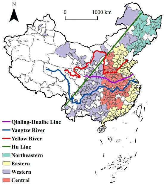
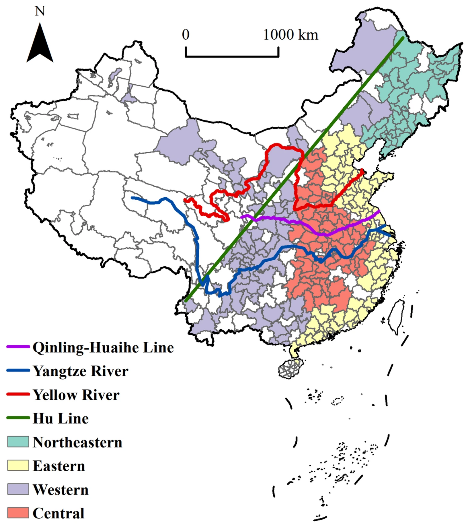
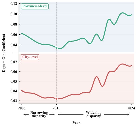
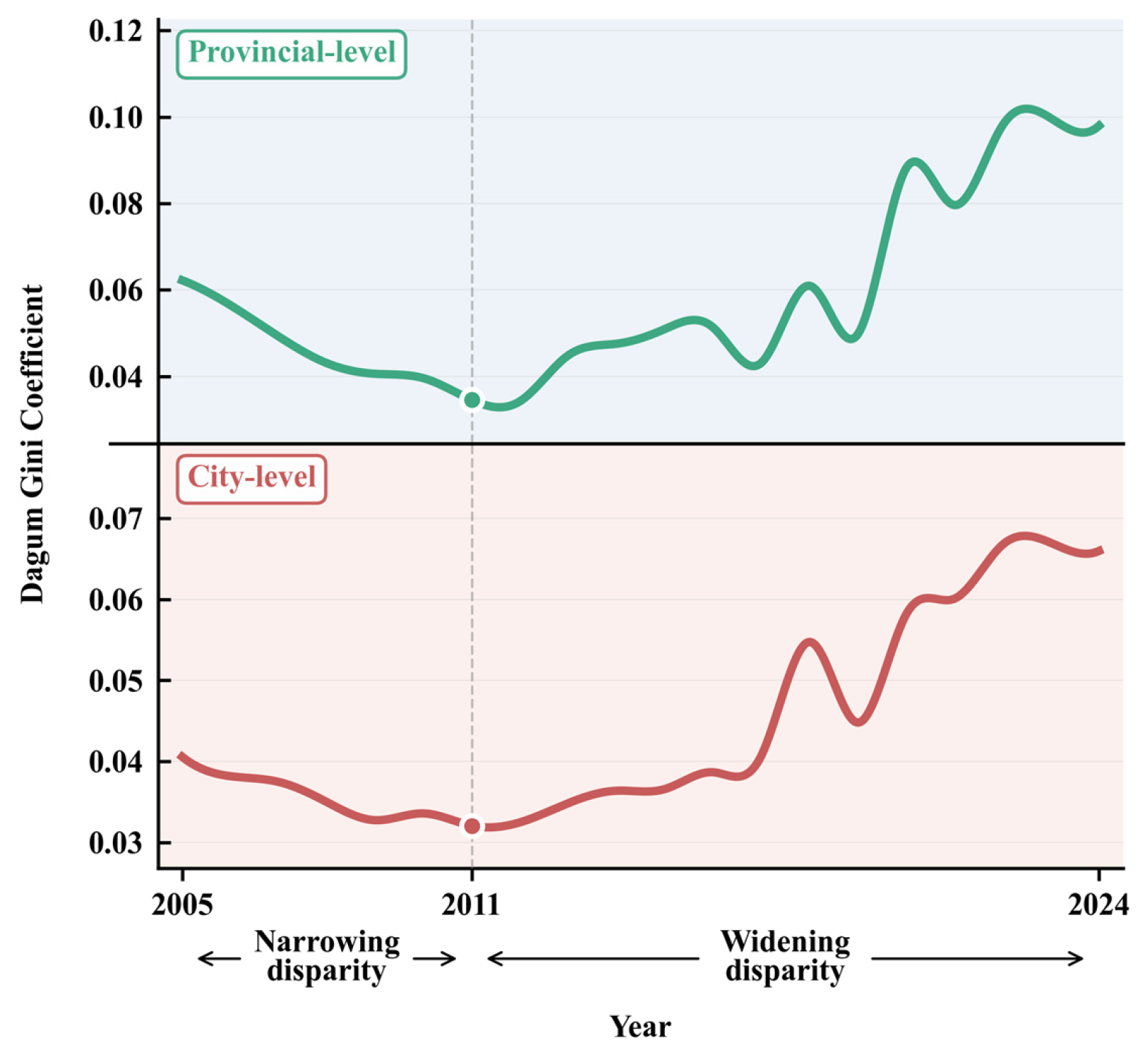
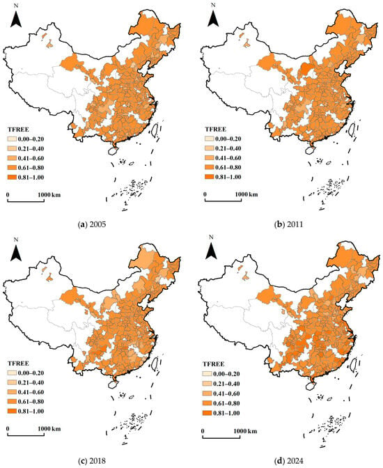
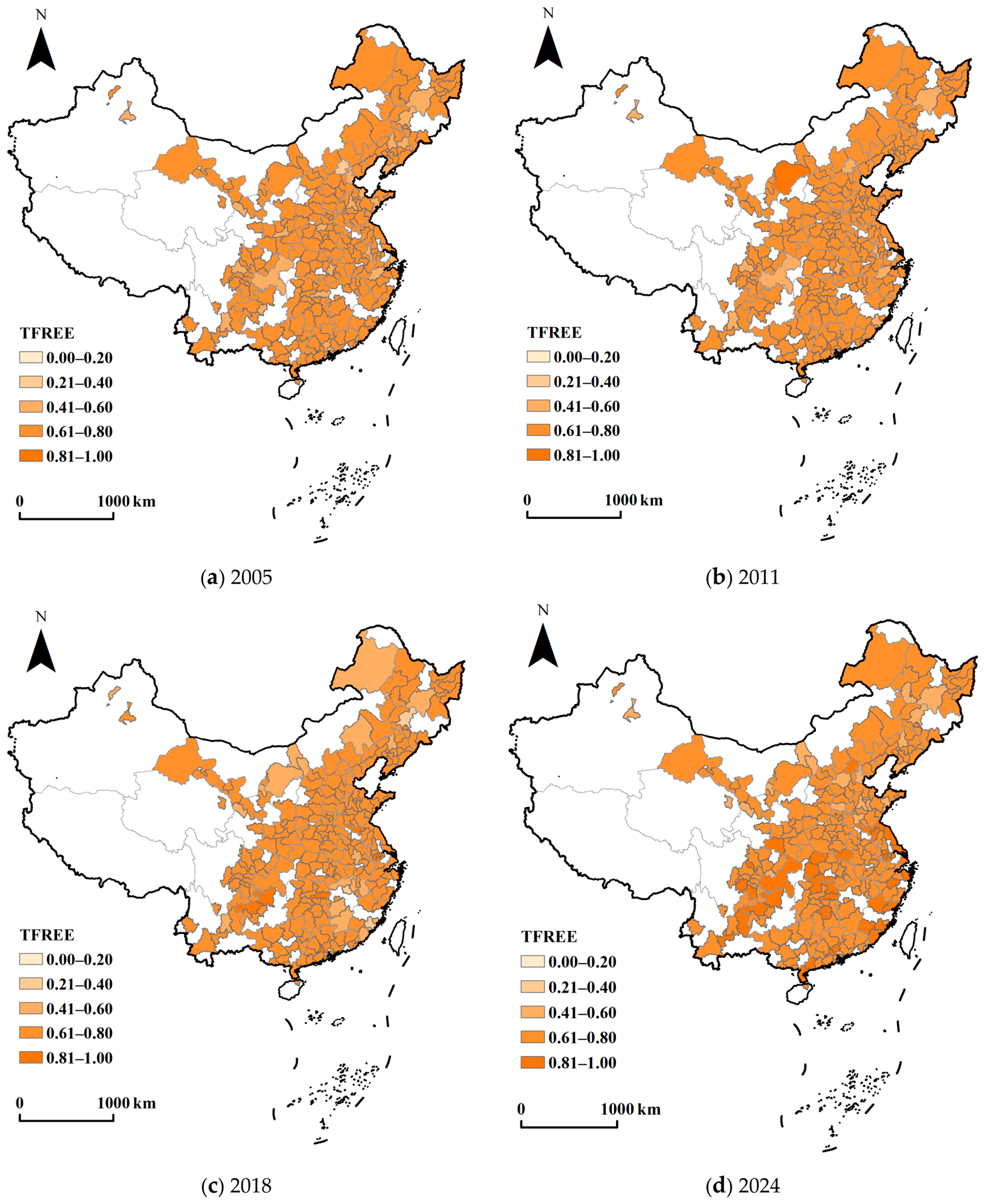
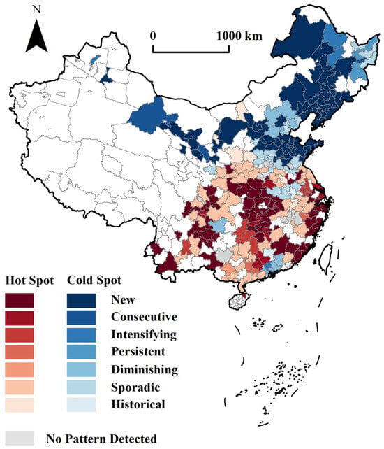
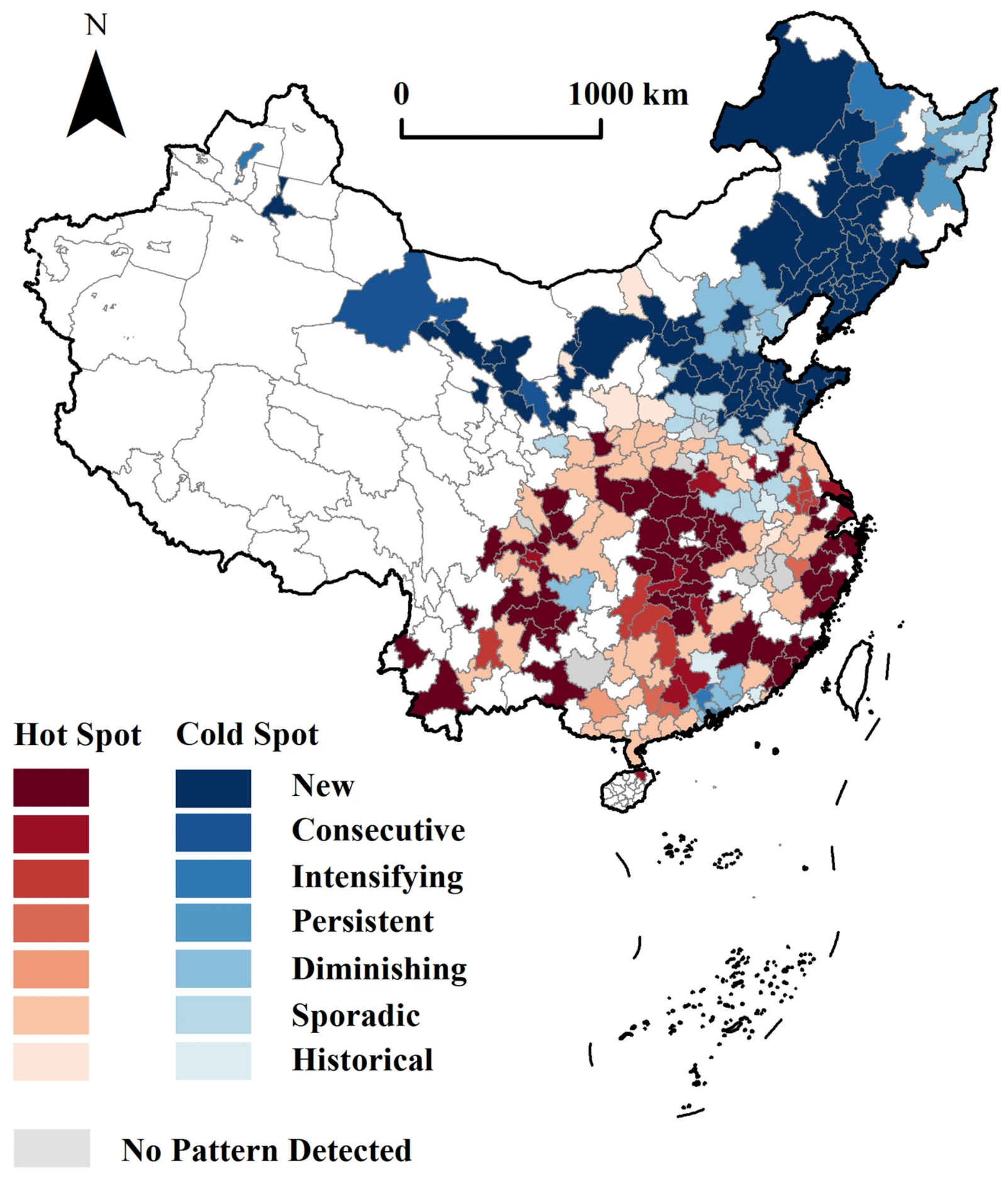
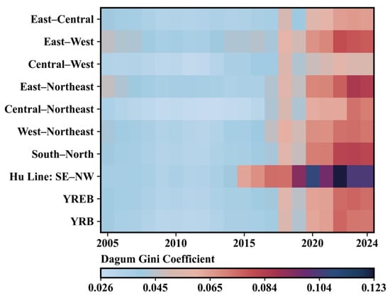
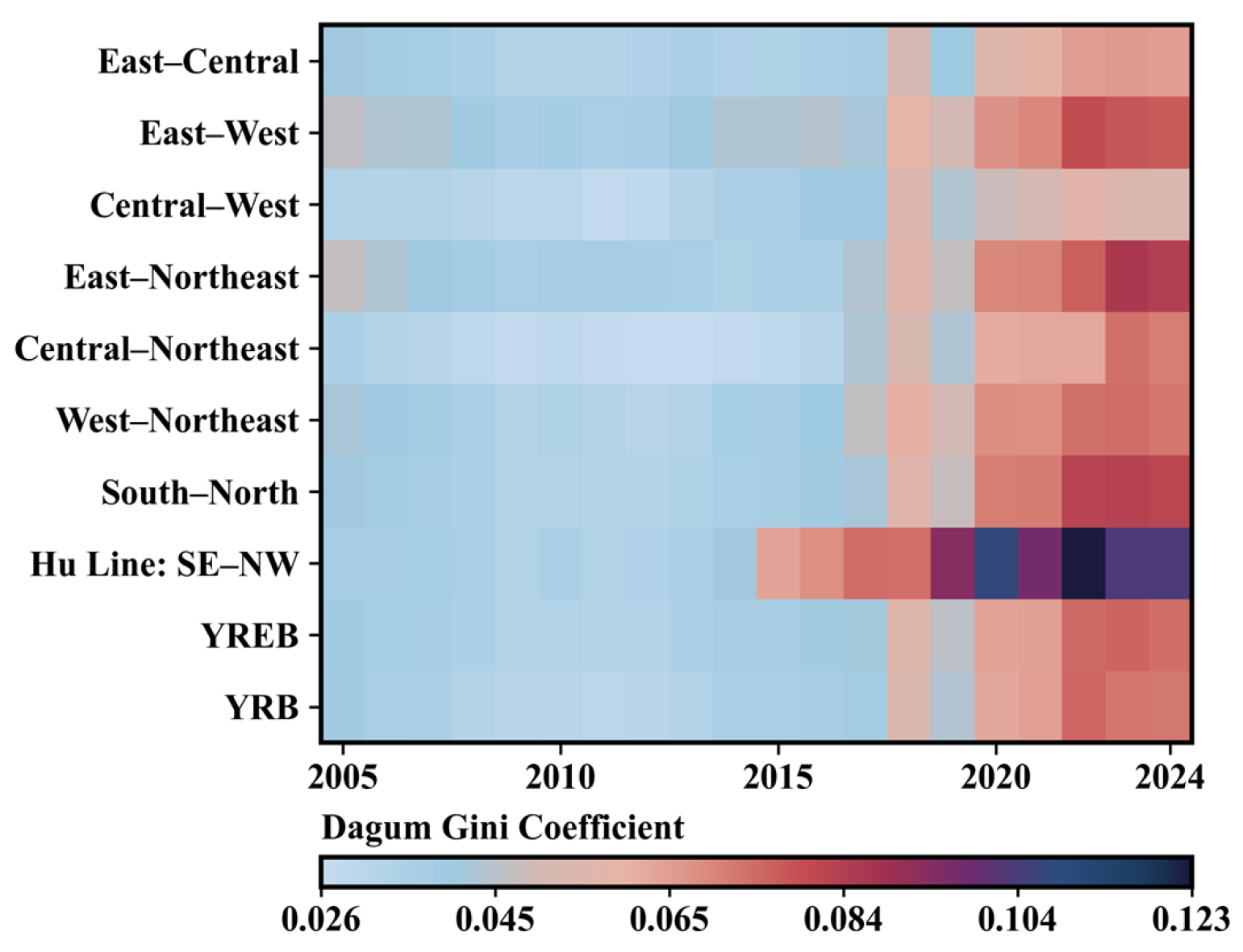
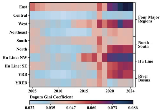
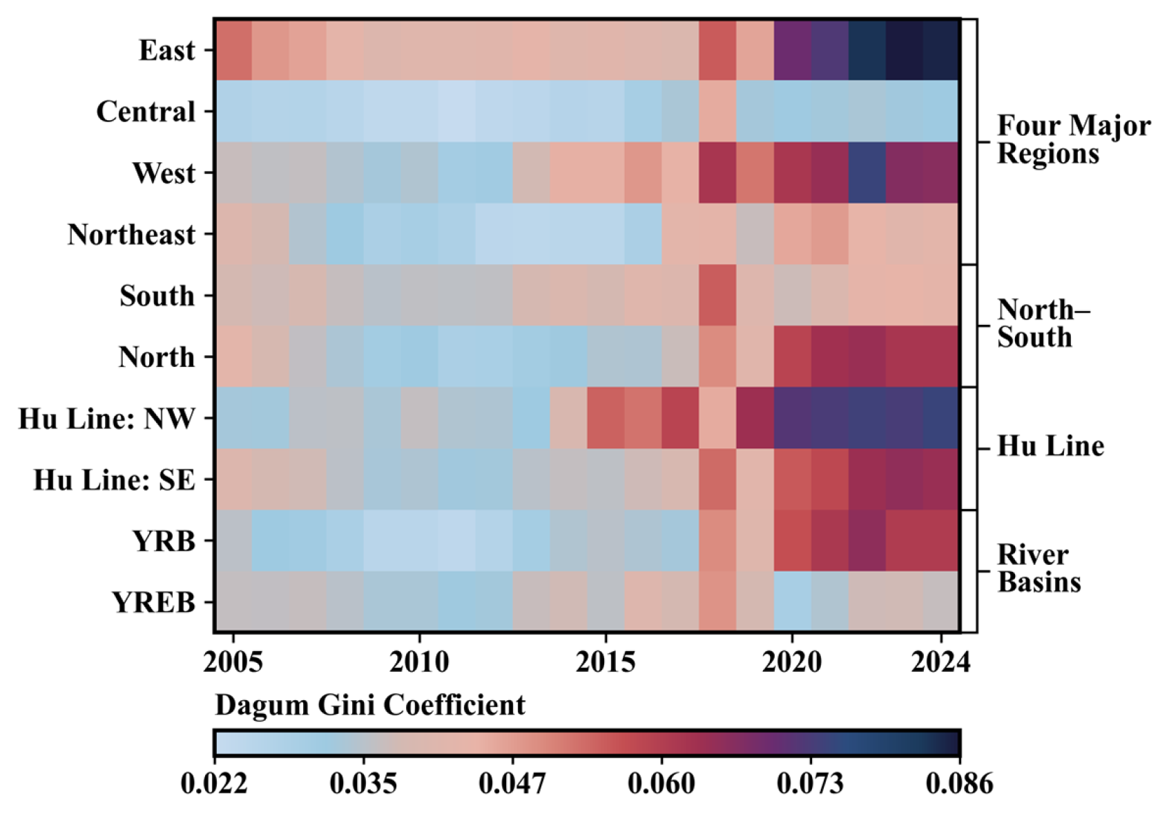
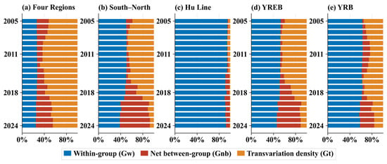
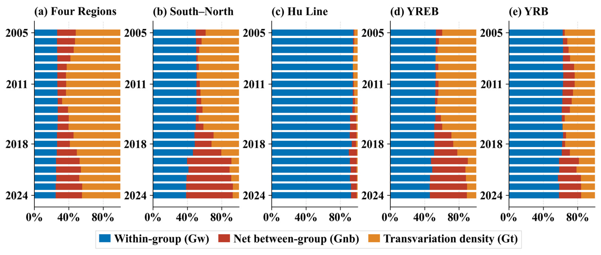
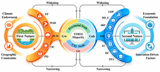
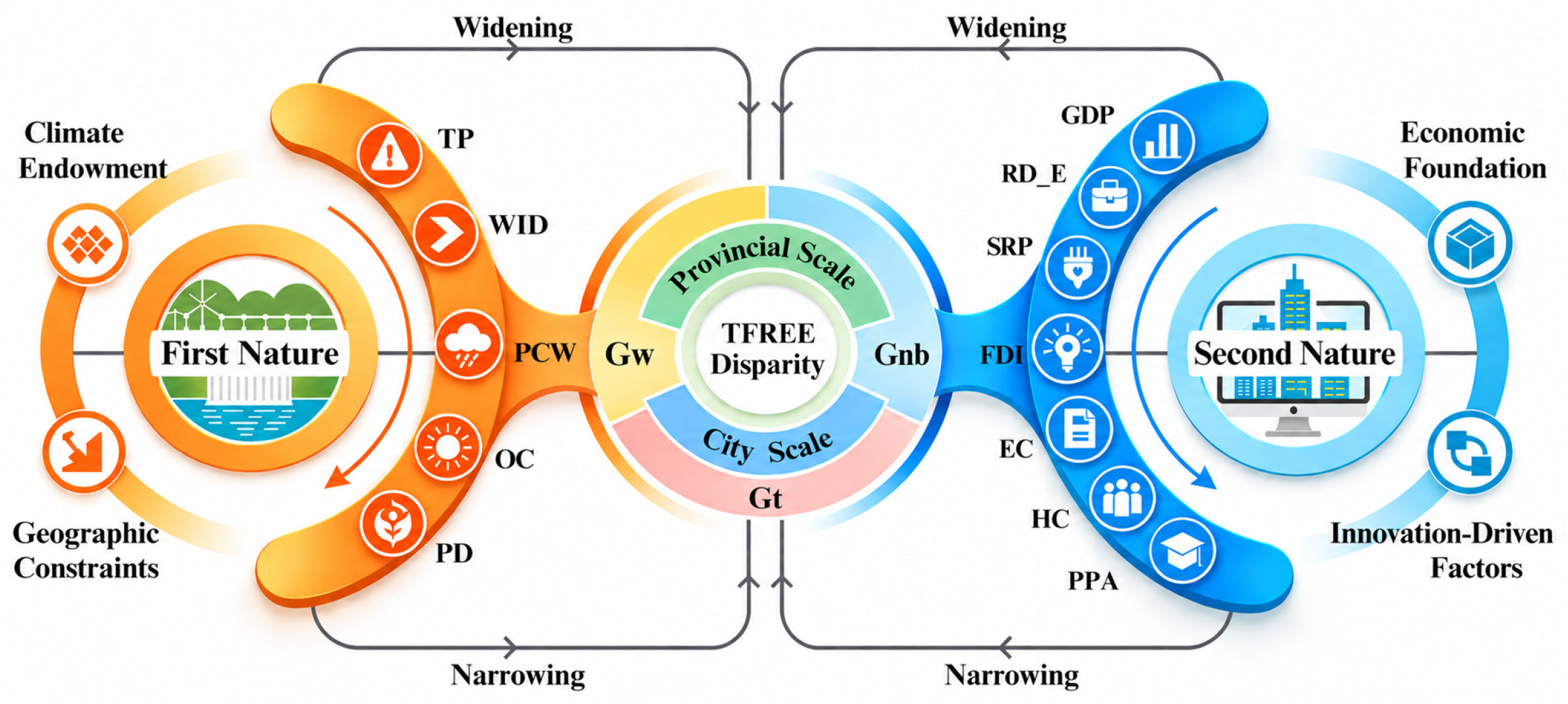
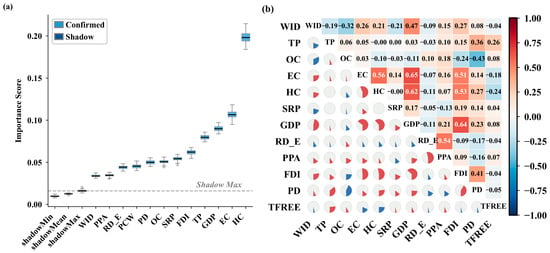
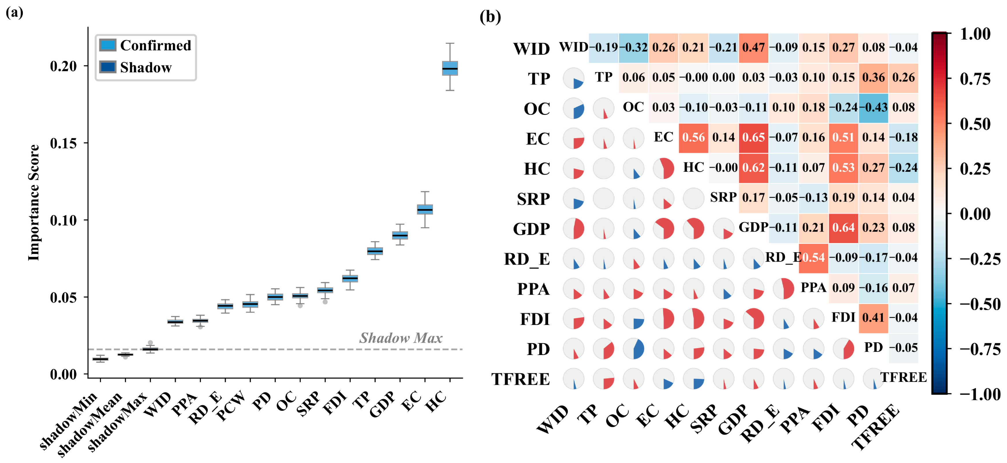
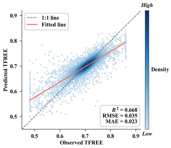
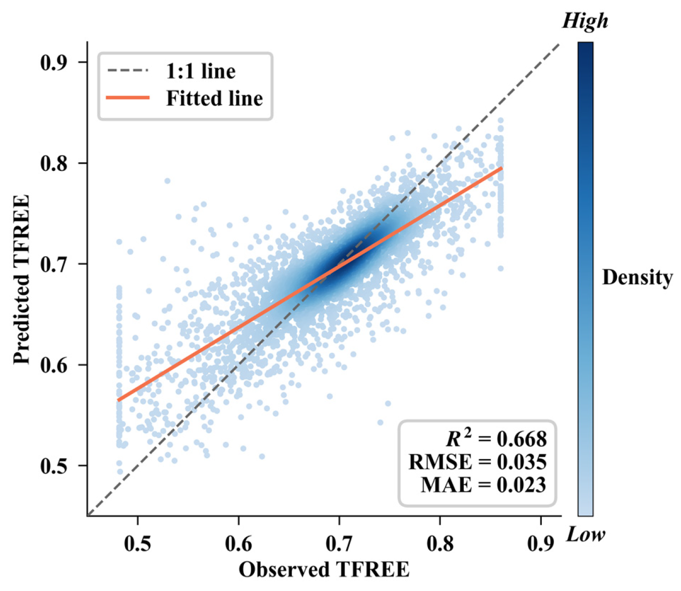
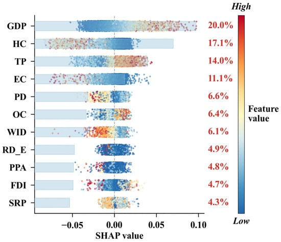
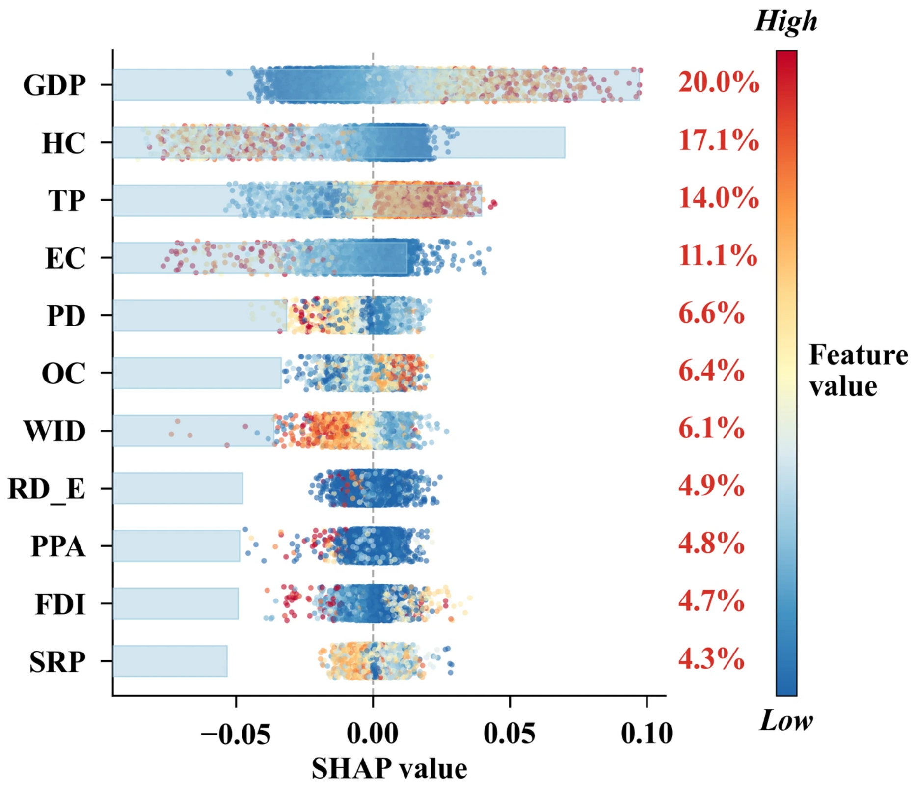
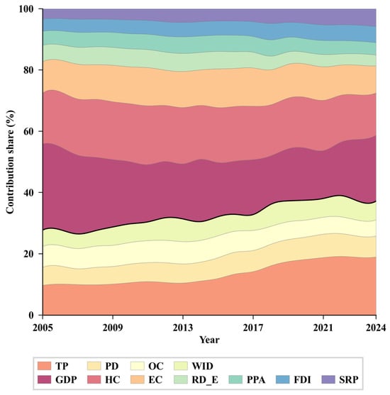
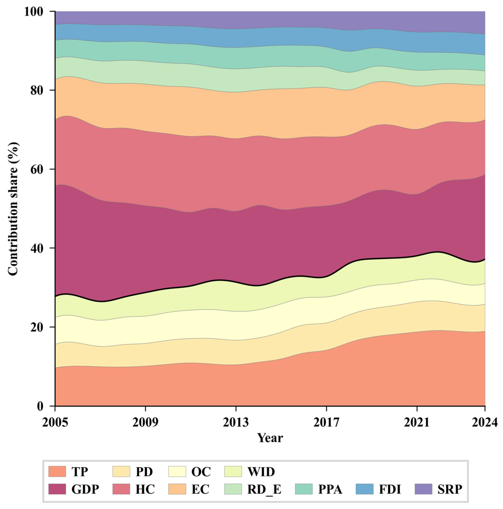
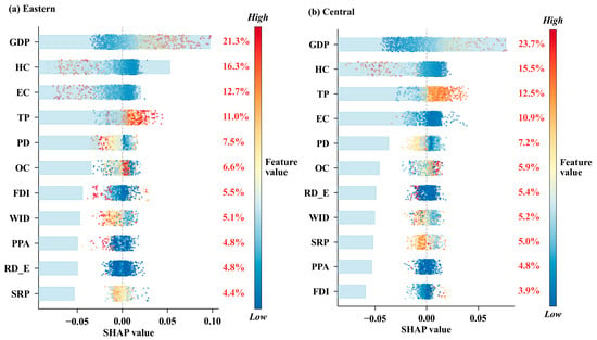
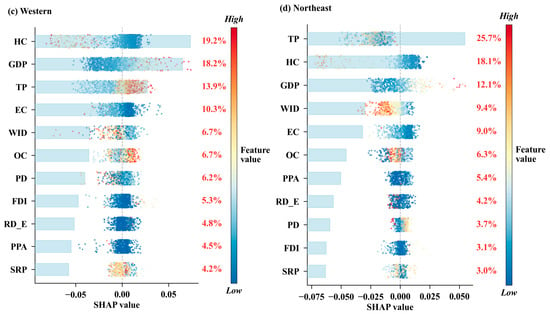
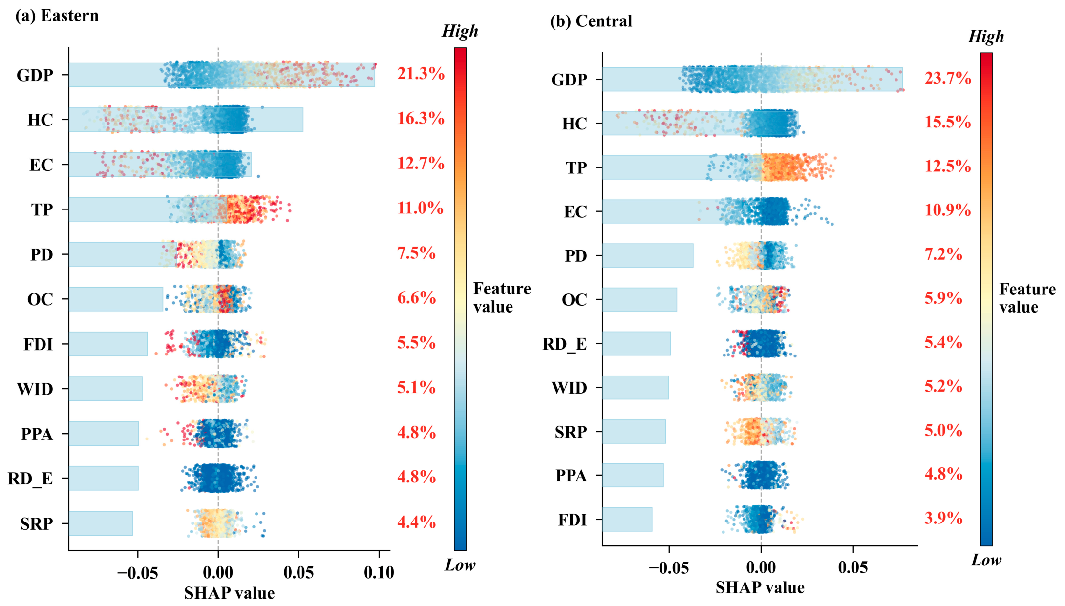
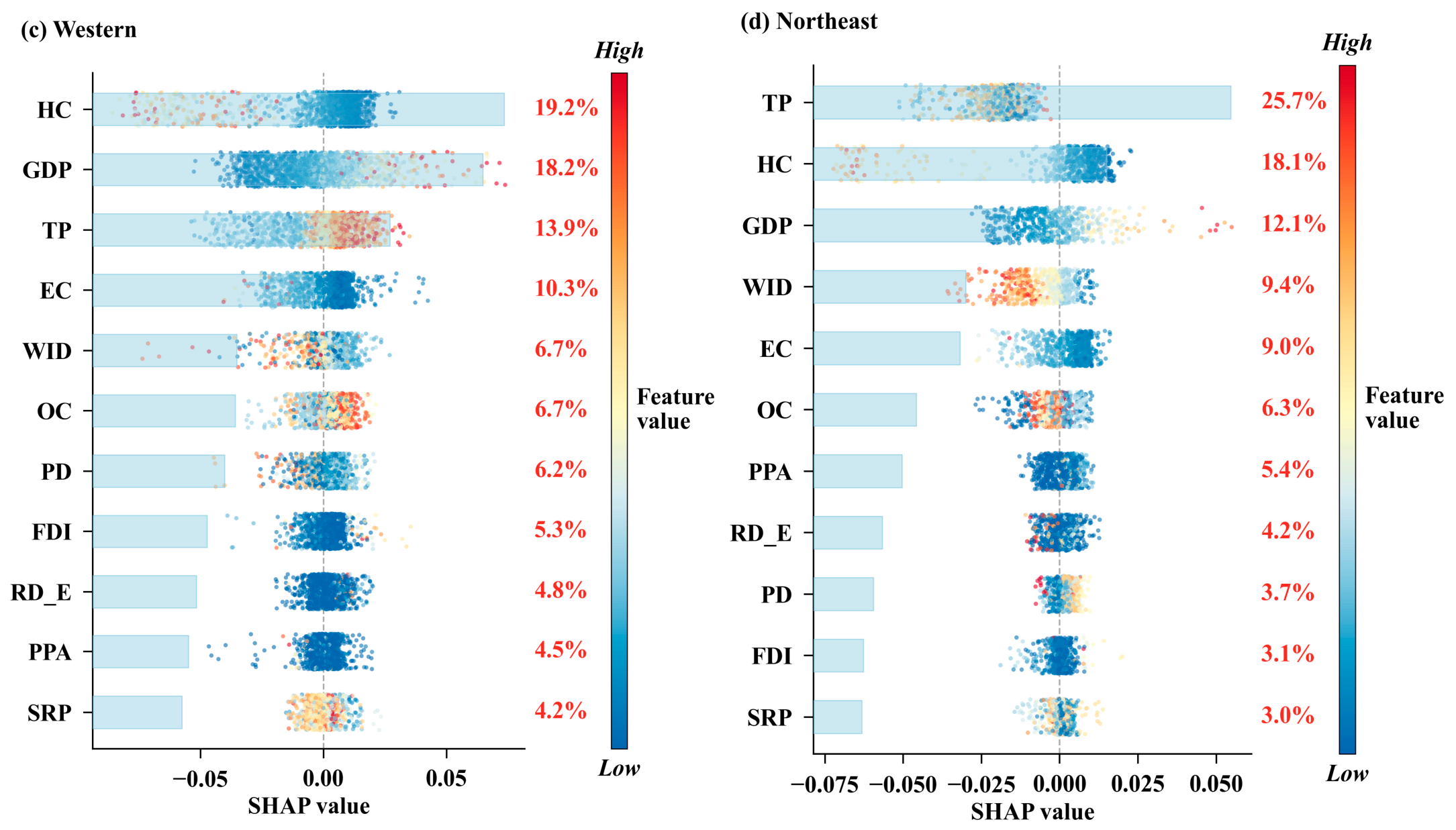
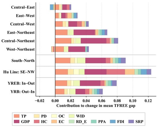
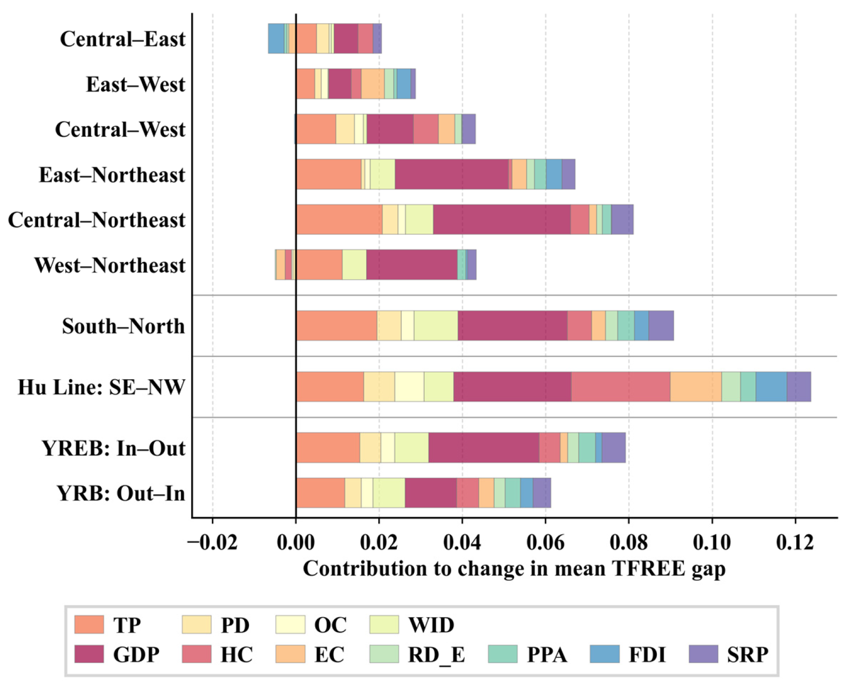
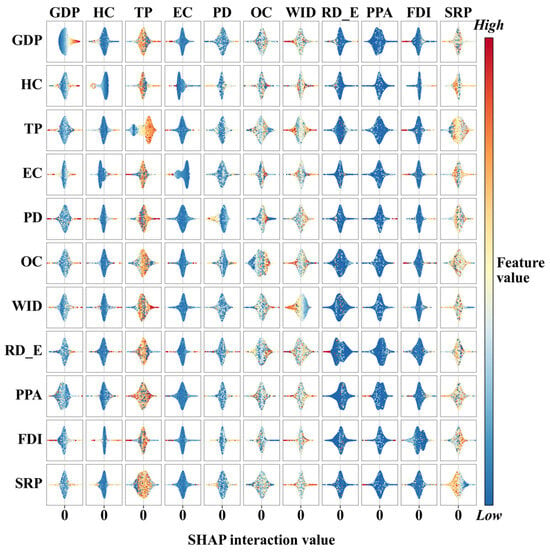
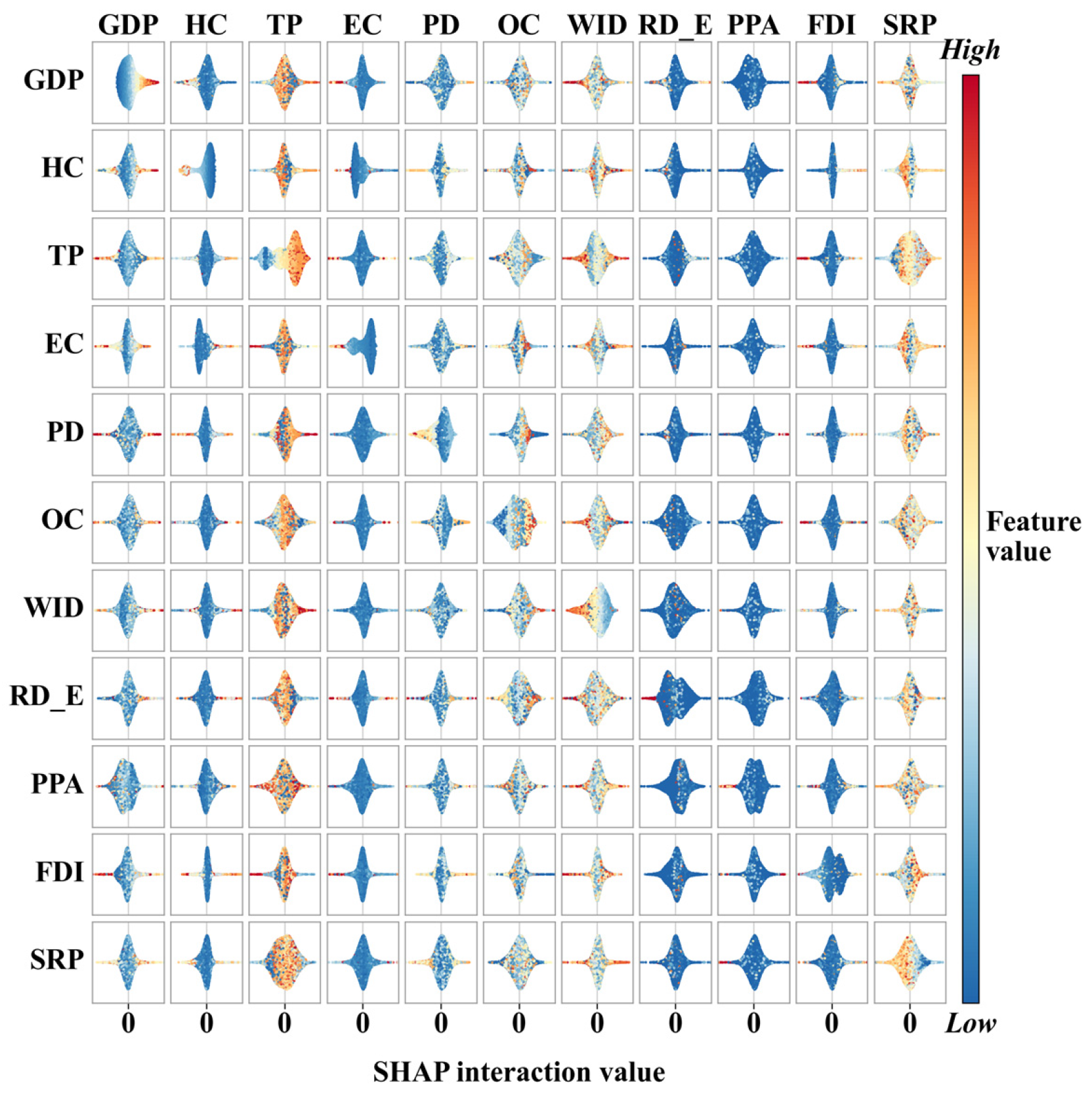
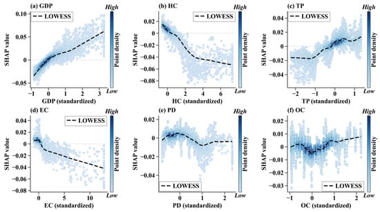
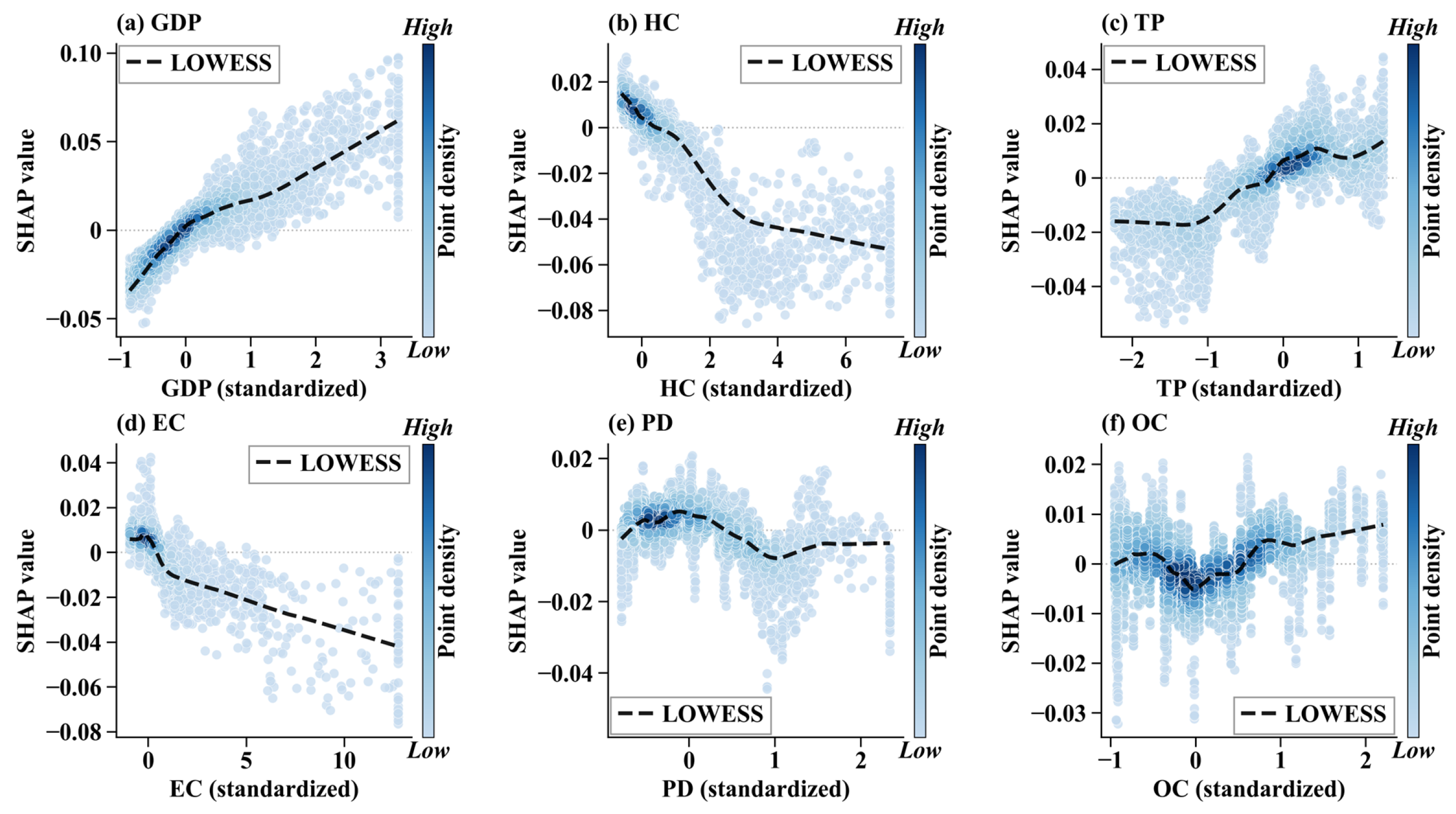
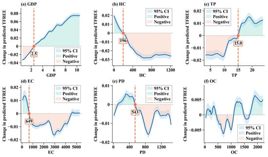
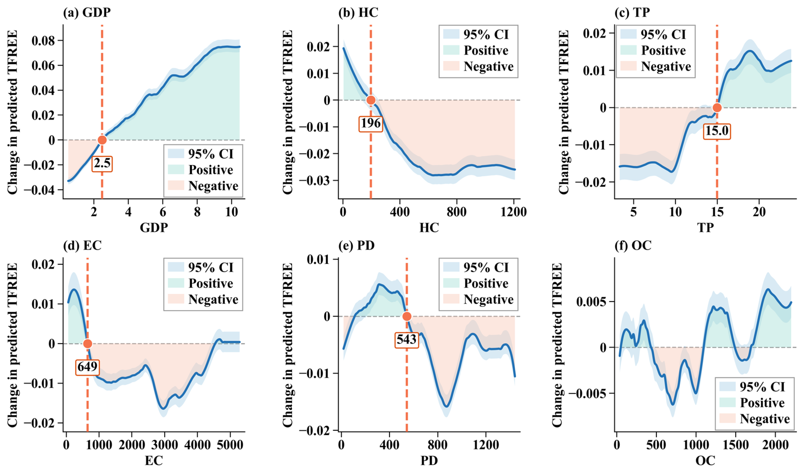
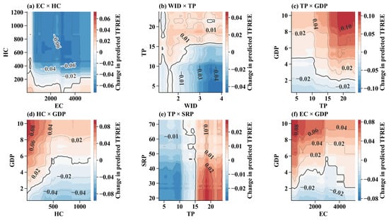
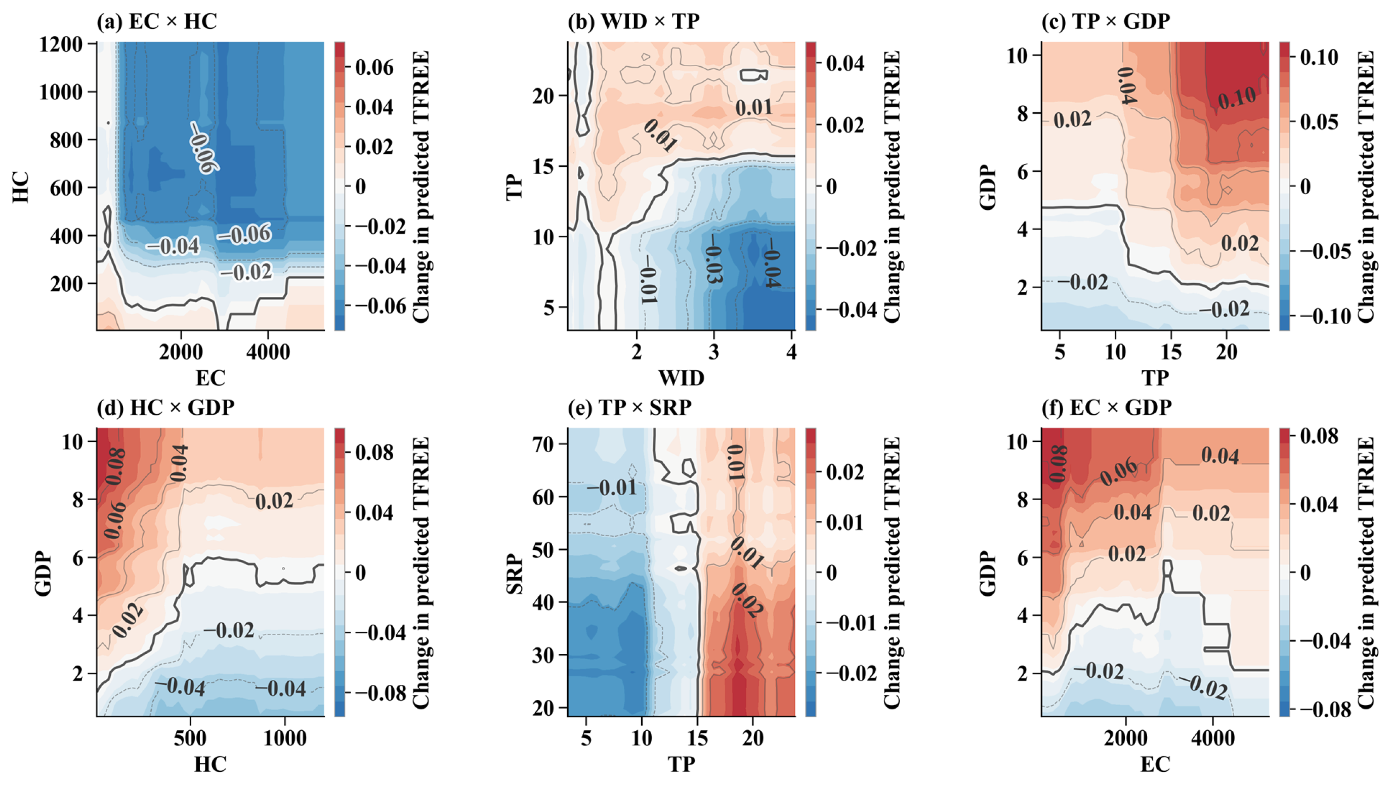

Disclaimer/Publisher’s Note: The statements, opinions and data contained in all publications are solely those of the individual author(s) and contributor(s) and not of MDPI and/or the editor(s). MDPI and/or the editor(s) disclaim responsibility for any injury to people or property resulting from any ideas, methods, instructions or products referred to in the content. |
© 2026 by the authors. Licensee MDPI, Basel, Switzerland. This article is an open access article distributed under the terms and conditions of the Creative Commons Attribution (CC BY) license.