Transient and Steady-State Gas Lift Transportation of Non-Newtonian Rare Earth Slurry: A Water–Gas–Slurry Modeling Study

Abstract

Gas lift transportation of deep-sea rare earth mud involves the replacement of initial water by a non-Newtonian suspension and substantial axial variation in gas content along a long riser. This study develops a one-dimensional drift flux formulation that distinguishes the initial internal water from the incoming power law slurry through liquid volume accounting and material property assignment. Gas compressibility, relative phase motion, and wall resistance are included. The staggered grid finite-volume solver is assessed through outlet scalar resolution comparisons, single-phase power law verification, and published air–water discharge experiments. The pooled discharge MARD is 5.79% for the air–water cases; the non-Newtonian slurry-lifting cases are model predictions without direct experimental validation. In a 6000 m riser, comparison of two liquid property treatments illustrates the sensitivity of the predicted start-up and late-time gas-holdup distributions. Increasing slurry concentration from 2% to 10% reduces volumetric throughput from approximately 0.750 to 0.651 m³/s and increases frictional pressure loss from approximately 0.257 to 0.899 MPa. Greater injection depth and gas mass flow increase throughput with diminishing incremental gains. The 3000 m and 8 kg/s cases achieve approximately 94.7% and 95.1% of their respective series reference throughputs. A separate outlet diagnostic retains homogeneous Mach indicators above unity at the outlet and final interior center and distinguishes these from the coupled drift flux characteristics. The results quantify the hydraulic effects of slurry rheology and gas supply while distinguishing bulk transport trends from the terminal outlet response.

1. Introduction

Rare earth elements (REEs) comprise the lanthanides, yttrium, and scandium and are important constituents of magnets, optical devices, and other advanced technologies [1,2,3]. Their resource distribution, supply chains, and environmental implications have motivated studies of alternative deposits [4,5,6,7]. REE-rich sediments around Minamitorishima in the western Pacific provide a marine resource whose mineralogy, enrichment, and occurrence have been investigated extensively [8,9,10,11,12]. Transporting these fine-grained sediments from the seabed to a surface facility is a central engineering requirement for their recovery.

A deep-sea mining system combines collection, preparation, and vertical transportation of the recovered material [13]. For fine rare earth mud, the transportation problem is closely connected to the rheology of its suspension [14]. Measurements of Minamitorishima mud mixed with seawater show concentration-dependent, shear-thinning behavior [15]. The power law representation used in rare earth mud airlift modeling [16] provides a practical relationship between shear stress and shear rate through the consistency coefficient K and flow behavior index n. Gas lift has consequently been considered within integrated recovery schemes for these resources [17].

In a gas lift riser, injected compressed gas reduces the mean density of the internal column relative to the surrounding water, generating a pressure difference that drives liquid upward. Experimental studies have examined the effects of geometry, submergence, and gas supply. Fan et al. [18] developed pumping rate correlations for artificial upwelling; Kim et al. [19] measured bubble patterns and discharge for different tube diameters and submergence ratios; Khalil et al. [20] compared injection arrangements; and Wang et al. [21] investigated a diffusion-driven bubble pump. Numerical studies provide complementary information on internal pressure, phase distribution, and velocity. Examples include gas lift liquid metal transportation [22] and deep-sea airlift modeling [23]. These studies establish the coupled roles of gas expansion, relative phase motion, and hydraulic resistance.

Rare earth slurry transportation requires material property distinctions beyond those represented in an air–water calculation. The external seawater determines the hydrostatic boundary, the submerged riser initially contains water, and the incoming slurry has concentration-dependent density and non-Newtonian resistance. During start-up, material replacement and gas injection evolve together. Studies of non-Newtonian two-phase flows also demonstrate the influence of shear-dependent liquid properties on deformation, breakup, bubble rise, and coalescence [24,25,26,27,28]. A one-dimensional riser description addresses their net effect on cross-sectionally averaged transportation through constitutive and drift relationships. The parent void-fraction-correlated framework has been compared with measured apparent velocities, gas volume fractions, and outlet pressure drop [29].

The present study represents the incoming rare earth slurry as a homogeneous power law suspension within a drift flux model. Liquid volume accounting distinguishes the initial internal water from the entering slurry; gas and the averaged liquid suspension are the moving phases. The parameters K and n enter the generalized Reynolds number and slurry wall resistance, while pressure-dependent gas density and drift couple the material properties to the axial hydraulics. The model is solved by a staggered finite-volume method with sequential pressure–velocity coupling. Its assessment combines outlet scalar spatial and temporal sensitivity, verification against an analytical single-phase shear-thinning solution, and validation of Newtonian air–water discharge. The parameter study then quantifies slurry throughput and frictional pressure loss for changes in concentration, injection depth, and gas mass input. An additional prescribed property calculation examines the terminal Mach indicator and coupled characteristics.

Section 2 defines the balances, material relationships, and closures. Section 3 specifies the geometry, initial and boundary conditions, and solution procedure. Section 4 presents the numerical and experimental assessments. Section 5 reports the material treatment comparison, the outlet diagnostic, and the three hydraulic parameter series. Section 6 summarizes the resulting transportation trends.

2. Mathematical Model

The riser is represented by a one-dimensional, cross-sectionally averaged drift flux model for gas and a liquid suspension. External seawater sets the surrounding hydrostatic pressure, while the liquid inside of the pipe is initially seawater and progressively replaced by incoming rare earth slurry. The water–gas–slurry terminology identifies these materials and their hydraulic roles. The following assumptions define the averaged description.

(1) The pipe is vertical with a constant circular cross-section of diameter D and area A = πD²/4. Axial coordinate z increases upward. Physical elevation relative to the external free surface is denoted as zp; the profile figures use z = 0 at their upper plotted reference. The two coordinates differ by a constant vertical offset, so their axial derivatives are identical.

(2) Pressure, gas holdup, and velocities are cross-sectionally averaged. The mud particles and carrier water move together as one homogeneous liquid suspension; the prescribed solids volume concentration CX determines its material properties. No additional solids concentration transportation equation or independently resolved water–slurry interface equation is introduced.

(3) The liquid is incompressible at a specified composition, the gas is compressible and ideal, and the temperature is constant. There is no phase change. Gas injection supplies mass to the mixture and gas equations.

(4) Local gas holdup selects and connects empirical drift relationships. The selected prescription combines bubbly and slug expressions with a specified interpolation interval. The separate large-diameter alternative includes an annular branch. These prescriptions are identified below so that the selected calculation and the reference alternative remain distinct.

2.1. Conservation Equations and Velocity Definitions

The solved fields are mixture mass, gas mass, and mixture momentum. Here, αg is the gas volume fraction, αl = 1 − αg is the liquid fraction, and ρm is the gas–liquid mixture density. The mixture mass balance is

$${\displaystyle \frac{\partial {\rho }_m}{\partial t}}+{\displaystyle \frac{\partial \left({\rho }_m{v}_m\right)}{\partial z}}={\Gamma }_m$$

(1)

The gas mass balance is

$${\displaystyle \frac{\partial \left({\alpha }_g{\rho }_g\right)}{\partial t}}+{\displaystyle \frac{\partial \left({\alpha }_g{\rho }_g{v}_g\right)}{\partial z}}={\Gamma }_g$$

(2)

With g denoting the positive magnitude of gravitational acceleration, the upward axial gravitational component is −g. The conservative mixture momentum balance is

$${\displaystyle \frac{\partial \left({\rho }_m{v}_m\right)}{\partial t}}+{\displaystyle \frac{\partial \left({\rho }_m{v}_m^2+p+S_d\right)}{\partial z}}=-{\rho }_{m}g-G_f$$

(3)

The gas and liquid intrinsic velocities vg and vl differ through the drift closure. The mass-averaged mixture velocity vm is distinct from the total volumetric flux j. The phase superficial velocities are jg = αgvg and jl = αlvl. The closure intercept vgj in vg = C0j + vgj is also distinct from the total gas drift VGj = vg − j. Expanding the sum of phase momentum fluxes about vm gives the relative motion contribution Sd below. Equation (3) therefore uses the total drift VGj rather than the intercept alone. Gf = 4τw/D is the signed wall friction pressure gradient, positive for upward flow and opposed by the minus sign in the momentum balance.

$${\rho }_m={\alpha }_g{\rho }_g+{\alpha }_l{\rho }_l, {\alpha }_l=1-{\alpha }_g$$

(4)

$$v_m={\displaystyle \frac{{\alpha }_g{\rho }_g{v}_g+{\alpha }_l{\rho }_l{v}_l}{{\rho }_m}}$$

(5)

$$j_g={\alpha }_g{v}_g, j_l={\alpha }_l{v}_l, j=j_g+j_l$$

(6)

$$v_g=C_{0}j+v_{gj}, V_{Gj}=v_g-j=\left(C_0-1\right)j+v_{gj}$$

(7)

$$S_d={\displaystyle \frac{{\alpha }_g{\rho }_g{\rho }_l}{{\alpha }_l{\rho }_m}}{V}_{Gj}^{\hspace{0.17em}2}={\displaystyle \frac{{\alpha }_g{\alpha }_l{\rho }_g{\rho }_l}{{\rho }_m}}{\left(v_g-v_l\right)}^2$$

(8)

The gas density is evaluated from absolute pressure as ρg = p/(RgT), where Rg is the specific gas constant and T is the prescribed absolute temperature. Consequently, decreasing pressure during ascent increases gas volumetric flux and couples gas expansion to holdup, drift, and mixture acceleration. The gas-free slurry density is ρsl = (1 − CX)ρw + CXρs, where ρw is seawater density and ρs is mud particle density. The value 2800 kg/m³ denotes ρs, not the density of the complete slurry. Local liquid property assignment during water replacement is described in Section 2.3. The ideal gas approximation sets Z = 1 in the general relation ρg = p/[Z(p,T)RgT]. The air equation of state of Lemmon et al. [30] provides the thermodynamic reference for distinguishing this approximation from the pressure-dependent gas compressibility retained in the model.

$${\rho }_g={\displaystyle \frac{p}{R_{g}T}}, {\rho }_{\mathrm{s}\mathrm{l}}=\left(1-C_X\right){\rho }_w+C_X{\rho }_s$$

(9)

The prescribed Z = 1 follows from the ideal gas assumption in Equation (9). Air is treated as an isothermal ideal gas at T = 293.15 K, so gas density varies with local absolute pressure. Real gas effects and their influence on gas density, gas holdup, and gas expansion at high pressure are not included, which constitutes a limitation of the present model. The hydraulic comparisons are interpreted within the scope of this isothermal ideal gas model.

2.2. Drift and Wall Resistance Closures

The selected bubbly–slug prescription uses the distribution coefficient C0 and dimensional drift intercepts below. Kajishima and Saito [31] supply the pipe-scale slug relationship and the 0.25–0.30 connection; the bubbly hindrance factor follows the distorted bubble drift treatment of Ishii [32], also summarized by Hatakeyama et al. [33]. Defining rρ = ρg/ρl, the dimensional velocity scale uσ has units m/s.

$$r_{\rho }={\displaystyle \frac{{\rho }_g}{{\rho }_l}}, u_{\sigma }={\left[{\displaystyle \frac{g\sigma \left({\rho }_l-{\rho }_g\right)}{{\rho }_l^2}}\right]}^{1/4}$$

(10)

$$C_0=1.2-0.2\sqrt{r_{\rho }}$$

(11)

$$v_b=\sqrt{2}\hspace{0.17em}{u}_{\sigma }{\left(1-{\alpha }_g\right)}^{1.75}, v_s=0.35\sqrt{{\displaystyle \frac{gD\left({\rho }_l-{\rho }_g\right)}{{\rho }_l}}}$$

(12)

The selected drift intercept is bubbly for αg ≤ 0.25, linearly interpolated for 0.25 < αg < 0.30, and the slug expression for αg ≥ 0.30. The last branch is retained as the high-holdup continuation of this prescription. These bounds specify the numerical constitutive selection; they do not constitute a separately resolved flow–pattern interface.

$$v_{gj}=\{\begin{array}{ll}{v}_b,& {\alpha }_g\le 0.25,\\ v_b+\left(v_s-v_b\right){\displaystyle \frac{{\alpha }_g-0.25}{0.05}},& 0.25<{\alpha }_g<0.30,\\ v_s,& {\alpha }_g\ge 0.30.\end{array}$$

(13)

For reference, the alternative large-diameter formulation summarized by Hatakeyama et al. [33], including the Kataoka–Ishii intermittent correlation [34], is specified in dimensionally explicit form below. A star denotes a dimensionless drift intercept, with vgj = uσvgj*. The capillary length ℓc, dimensionless diameter ND, and viscosity number Nμ are defined using a dynamic liquid viscosity μl in Pa·s. K, which has units of Pa·sⁿ, is not substituted directly for μl. This viscosity-dependent alternative is separate from the selected bubbly–slug prescription.

$${\mathcal{l}}_c=\sqrt{{\displaystyle \frac{\sigma }{g\left({\rho }_l-{\rho }_g\right)}}}, N_D={\displaystyle \frac{D}{{\mathcal{l}}_c}}, N_{\mu }={\displaystyle \frac{{\mu }_l}{\sqrt{{\rho }_l\sigma {\mathcal{l}}_c}}}, v_{gj}=u_{\sigma }{v}_{gj}^{*}$$

(14)

$$C_{0,B}=\left(1.2-0.2\sqrt{r_{\rho }}\right)\left(1-e^{-18{\alpha }_g}\right), v_{gj,B}^{*}=\sqrt{2}{\left(1-{\alpha }_g\right)}^{1.75}$$

(15)

$$C_{0,I}=1.2-0.2\sqrt{r_{\rho }}$$

(16)

$$v_{gj,I}^{*}=\{\begin{array}{ll}0.0019N_D^{0.809}{r_{\rho }}^{-0.157}{N}_{\mu }^{-0.562},& N_{\mu }\le 2.25\times {10}^{-3},N_D\le 30,\\ 0.030{r_{\rho }}^{-0.157}{N}_{\mu }^{-0.562},& N_{\mu }\le 2.25\times {10}^{-3},N_D>30,\\ 0.92{r_{\rho }}^{-0.157},& N_{\mu }>2.25\times {10}^{-3},\end{array}$$

(17)

$$C_A={\displaystyle \frac{1-{\alpha }_g}{{\alpha }_g+\sqrt{\frac{\left[1+75\left(1-{\alpha }_g\right)\right]{\rho }_g}{\sqrt{{\alpha }_g}{\rho }_l}}}}, C_{0,A}=1+C_A, v_{gj,A}^{*}=C_A\sqrt{{\displaystyle \frac{\left(1-{\alpha }_g\right)N_D}{0.015}}}$$

(18)

The alternative uses the bubbly expression through αg = 0.20, interpolation over 0.20–0.30, the intermittent expression over 0.30–0.70, interpolation over 0.70–0.80, and the annular expression from 0.80. Interpolation connects both C0 and the drift intercept. The starred annular expression must be multiplied by uσ to obtain m/s. The coefficient 0.92 is only the high-Nμ intermittent branch. The selected drift prescription instead couples slurry rheology through the K, n-dependent wall resistance and the resulting pressure, fluxes, and holdup, consistent with the rare earth mud drift flux/power law modeling approach of Shimizu et al. [16].

Wall resistance is expressed as a pressure gradient Gf (Pa/m), with wall shear stress τw = DGf/4 (Pa). Newtonian reference resistance uses the Lockhart–Martinelli/Chisholm–Laird form assembled for airlift calculations by Hatakeyama et al. [33]. Writing Gk0 for the single-phase contribution based on phase superficial velocity jk, the upward-flow relationships are

$$G_f^{\mathrm{r}\mathrm{e}\mathrm{f}}=G_{l0}+G_{g0}+C_f\sqrt{\left|G_{l0}{G}_{g0}\right|}, C_f=83N_D^{-0.37}$$

(19)

$$G_{k0}={\displaystyle \frac{f_{D,k}{\rho }_k{j}_k\left|j_k\right|}{2D}}, R{e}_k={\displaystyle \frac{{\rho }_{k}D\left|j_k\right|}{{\mu }_k}}, k=g,l$$

(20)

$${\displaystyle \frac{1}{\sqrt{f_{D,k}}}}=-2{\mathrm{l}\mathrm{o}\mathrm{g}}_{10}\left({\displaystyle \frac{\epsilon /D}{3.71}}+{\displaystyle \frac{2.51}{R{e}_k\sqrt{f_{D,k}}}}\right)$$

(21)

Here, fD is the Darcy friction factor and ε is absolute wall roughness in meters; ε/D is dimensionless relative roughness. The water resistance branch has Gf,w = fD,wρljl|jl|(1 − αg)^−1.75/(2D). Its smooth pipe coefficient uses the explicit turbulent relationship of Fang, Xu, and Zhou [35]; the Colebrook equation above identifies the Newtonian rough pipe reference. These Newtonian relations are distinguished from the selected power law slurry branch in Section 2.3.

$$G_{f,w}={\displaystyle \frac{f_{D,w}{\rho }_l{j}_l\left|j_l\right|}{2D{\left(1-{\alpha }_g\right)}^{1.75}}}$$

(22)

$$f_{D,w}=0.25{\left[{\mathrm{l}\mathrm{o}\mathrm{g}}_{10}\left(150.39R{e}_l^{-0.98865}-152.66R{e}_l^{-1}\right)\right]}^{-2}$$

(23)

2.3. Slurry Rheology and Liquid Property Assignment

The incoming slurry obeys the power law relationship below, where K is consistency (Pa·sⁿ), n is dimensionless, and n < 1 denotes shear thinning. The apparent viscosity depends on the shear rate. The concentration fits are the empirical rare earth mud expressions reported by Shimizu, Hatakeyama, and Masuyama [16] for the measured mud suspension family. They use CX as a solids volume fraction over 0–10%. The SI numerical convention is written dimensionally using the reference rate $\dot{\mathsf{\gamma }}$0 = 1 s⁻¹, preserving the reported numerical values of K. The lower-concentration n branch applies through CX = 0.05.

$$\tau =K{\left|\dot{\gamma }\right|}^{n-1}\dot{\gamma }, {\mu }_{\mathrm{a}\mathrm{p}\mathrm{p}}=K{\left|\dot{\gamma }\right|}^{n-1}$$

(24)

$$K={\mu }_w{\dot{\gamma }}_0^{\hspace{0.17em}1-n}\left(8.91\times {10}^6{C}_X^{2.83}+1\right), {\dot{\gamma }}_0=1{\mathrm{s}}^{-1}, {\mu }_w=1.3\times {10}^{-3}\mathrm{P}\mathrm{a}\hspace{0.17em}s$$

(25)

$$n=\{\begin{array}{ll}1-1.85C_X^{0.282},& 0\le C_X\le 0.05,\\ 0.237-0.639C_X,& 0.05<C_X\le 0.10,\end{array}$$

(26)

$${\mu }_{\mathrm{e}\mathrm{q}}={\mu }_w\left(1+{\displaystyle \frac{3C_X}{1-C_X/0.52}}\right)$$

(27)

The Mori–Ototake relationship μeq, reproduced by Shimizu et al. [16], is an equivalent Newtonian comparison; it is distinct from μapp and is not substituted into the active power law resistance. For upward slurry transportation, K and n enter the Metzner–Reed generalized Reynolds number [36]. The selected finite Reynolds number slurry branch uses the resistance coefficient β and holdup multiplier below; β has the normalization stated in these equations. The empirical branch is evaluated for ReMR ≥ 100. Its numerical cutoff below this threshold is assessed against the laminar physical reference after Equation (31).

Initial water replacement is represented by liquid volume accounting. The accumulated liquid inlet volume locates the portion occupied by incoming slurry in the axial liquid inventory. Let χ denote its occupied fraction in a cell or staggered momentum volume. Fully replaced volumes use slurry properties and unreplaced volumes retain water properties. Partially replaced volumes use ρl = (1 − χ)ρw + χρsl and the corresponding weighted water/slurry resistance. K and n remain the prescribed slurry inputs; no fitted effective power law for an independently moving water–slurry mixture is introduced.

$$R{e}_{MR}={\displaystyle \frac{{\rho }_l{D}^n{j}_l^{\hspace{0.17em}2-n}}{K{8}^{n-1}{\left[\left(3n+1\right)/\left(4n\right)\right]}^n}}, j_l={\alpha }_l{v}_l\ge 0$$

(28)

$$\beta =1.32R{e}_{MR}^{-0.65}{\left(1-{\alpha }_g\right)}^{0.75}$$

(29)

$$G_{f,\mathrm{s}\mathrm{l}}={\displaystyle \frac{\beta {\rho }_l{j}_l\left|j_l\right|}{8D{\left(1-{\alpha }_g\right)}^{1.75}}}={\displaystyle \frac{1.32R{e}_{MR}^{-0.65}{\rho }_l{j}_l\left|j_l\right|}{8D\left(1-{\alpha }_g\right)}}, R{e}_{MR}\ge 100$$

(30)

$${\rho }_l=\left(1-\chi \right){\rho }_w+\chi {\rho }_{\mathrm{s}\mathrm{l}}, G_f=\left(1-\chi \right)G_{f,w}+\chi G_{f,\mathrm{s}\mathrm{l}}, 0\le \chi \le 1$$

(31)

The condition Gf,sl = 0 for ReMR < 100 is a numerical cutoff of the empirical finite Reynolds number branch. It prevents extrapolation of that branch below its imposed threshold; it does not represent a physical frictionless flow regime. A moving power law slurry retains wall friction. For fully developed, gas-free laminar flow, the appropriate physical reference is [36]

$${\mathrm{f}}_{\mathrm{D},\mathrm{l}\mathrm{a}\mathrm{m}}={\displaystyle \frac{64}{{\mathrm{R}\mathrm{e}}_{\mathrm{M}\mathrm{R}}}},{\mathrm{G}}_{\mathrm{l}\mathrm{a}\mathrm{m}}={\displaystyle \frac{4\mathrm{K}}{\mathrm{D}}}{\left[{\displaystyle \frac{3\mathrm{n}+1}{4\mathrm{n}}}{\displaystyle \frac{8{\mathrm{j}}_{\mathrm{l}}}{\mathrm{D}}}\right]}^{\mathrm{n}}.$$

(32)

This pressure gradient tends continuously to zero as jl tends to zero. The cutoff acts on the χ-weighted slurry contribution in Equation (31); the unreplaced volume uses the separate water branch. A representative start-up diagnostic uses L = 6000 m, D = 0.20 m, Hout = 4 m, hinj = 3000 m, CX = 0.10, a smooth pipe, gas input 10 kg/s with a 60 s ramp, N = 600, Δt = 0.6 s, and σ = 0.0728 N/m. The first positive slurry occupancy occurs at t = 119.4 s when χ = 0.166, the assigned local liquid density is 1049.56 kg/m³, and ReMR = 209. The empirical slurry friction branch is therefore already active at slurry entry in this diagnostic. This check concerns the onset of slurry entry, rather than every subsequent flow state. For fully replaced, gas-free 10% slurry in the same pipe, Equation (32) gives 679.7 Pa/m at ReMR = 100 or 5.8% of ρslg. This force-scale comparison is not a discharge error bound. Quantitative creeping flow start-up lies outside of the scope of the retained cutoff treatment; Equation (32) provides its physical reference.

3. Numerical Method

3.1. Geometry, Initial Conditions, and Boundaries

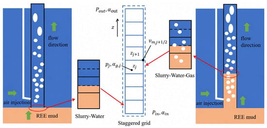
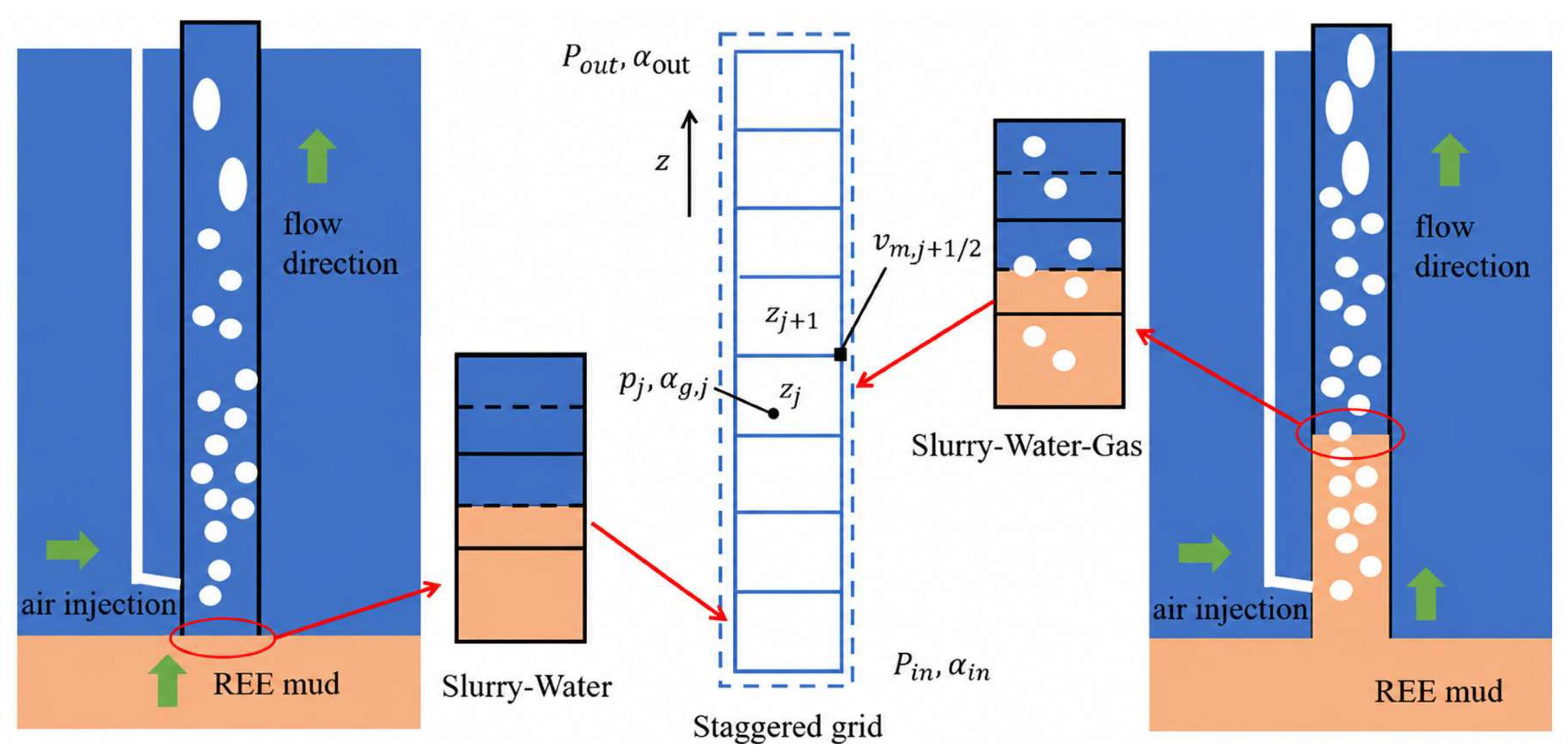
The vertical computational domain extends from the bottom inlet to the outlet. Its total length is L = Hs + Hout, where Hs is the submerged length and Hout is the outlet elevation above the external free surface. Injection depth hinj is measured downward from that surface, so zp,inj = −hinj; it is distinct from the suction length Hs − hinj below the injector. The submergence ratio is S = Hs/L. The external hydrostatic head is balanced by the internal mixture gravitational requirement, wall resistance, and momentum flux changes. Gas expansion couples this balance to holdup, so submergence and injection depth enter the hydraulic response through different geometric roles. Figure 1 defines this configuration.

$$S={\displaystyle \frac{H_s}{H_s+H_{\mathrm{o}\mathrm{u}\mathrm{t}}}}, z_{p,\mathrm{i}\mathrm{n}}=-H_s, z_{p,\mathrm{o}\mathrm{u}\mathrm{t}}=H_{\mathrm{o}\mathrm{u}\mathrm{t}}, z_{p,\mathrm{i}\mathrm{n}\mathrm{j}}=-h_{\mathrm{i}\mathrm{n}\mathrm{j}}$$

(33)

Figure 1. Gas lift system configuration and one-dimensional staggered grid arrangement. Blue, orange and white denote seawater, slurry and gas, respectively; the dashed lines mark the water–slurry boundaries in the insets and the outline of the staggered computational grid.

The reference physical properties are listed in Table 1. The prescribed liquid composition sets ρsl, K, and n, while gas density follows the local absolute pressure and fixed temperature.

Table 1. Material properties and isothermal gas specification.

Material/Quantity	Symbol	Specification
Air density	ρg	p/(RgT), kg/m3
Specific gas constant	Rg	287 J/(kg·K)
Temperature	T	293.15 K
Air dynamic viscosity	μg	1.76 × 10−5 Pa·s
Gas–liquid surface tension	σ	7.4 × 10−2 N/m
Seawater density	ρw	1020 kg/m3
Seawater dynamic viscosity	μw	1.3 × 10−3 Pa·s
Mud particle density	ρs	2800 kg/m3
Incoming slurry solids volume fraction	CX	0–0.10
Gas-free slurry density	ρsl	(1 − CX)ρw + CXρs
Gravitational acceleration magnitude	g	9.80 m/s2

The submerged pipe initially contains stationary, gas-free seawater with hydrostatic pressure p = patm − ρwgzp. The above-water portion fills during start-up. Incoming slurry enters through the gas-free bottom inlet as the pressure-driven inflow develops; its accumulated volume provides the liquid property assignment described above. The external seawater density supplies the inlet hydrostatic head even after the internal liquid is replaced by slurry.

The full-domain pressure boundaries are pin = patm + ρwgHs and pout = patm exp[−gHout/(RgT)], with patm = 101,325 Pa. During freeboard filling, the current liquid surface elevation replaces Hout in the outlet expression; once the pipe discharges, the geometric outlet elevation is used. These are prescribed absolute pressures, and the pressure corrections at both boundaries are zero. The inlet gas fraction is zero; outlet holdup is extrapolated from the adjacent interior values rather than prescribed to remain zero.

Gas is introduced uniformly within the injection control volume of area A and axial width Δzinj. The source increases linearly over 60 s to the prescribed gas mass input. Γm = Γg because there is no separate liquid volume source or phase change inside of the pipe. The lateral injection has zero imposed axial momentum. The reference deep-sea geometry and investigated parameter ranges are listed in Table 2.

$$p\left(z_p,0\right)=p_{\mathrm{a}\mathrm{t}\mathrm{m}}-{\rho }_{w}g{z}_p, v_m\left(z_p,0\right)=0, {\alpha }_g\left(z_p,0\right)=0 \left(z_p\le 0\right)$$

(34)

$$p_{\mathrm{i}\mathrm{n}}=p_{\mathrm{a}\mathrm{t}\mathrm{m}}+{\rho }_{w}g{H}_s, p_{\mathrm{o}\mathrm{u}\mathrm{t}}=p_{\mathrm{a}\mathrm{t}\mathrm{m}}\mathrm{e}\mathrm{x}\mathrm{p}\left(-{\displaystyle \frac{g{H}_{\mathrm{o}\mathrm{u}\mathrm{t}}}{R_{g}T}}\right)$$

(35)

$${\dot{m}}_g\left(t\right)={\dot{m}}_{g,\mathrm{m}\mathrm{a}\mathrm{x}}\mathrm{m}\mathrm{i}\mathrm{n}\left({\displaystyle \frac{t}{60\mathrm{s}}},1\right)$$

(36)

$${\Gamma }_g={\Gamma }_m=\{\begin{array}{ll}{\dot{m}}_g\left(t\right)/\left(A\Delta z_{\mathrm{i}\mathrm{n}\mathrm{j}}\right),& \mathrm{in}\mathrm{the}\mathrm{injection}\mathrm{cell},\\ 0,& \mathrm{elsewhere},\end{array} \left[{\Gamma }_g\right]=\mathrm{k}\mathrm{g}\hspace{0.17em}{m}^{-3}\hspace{0.17em}{s}^{-1}$$

(37)

Table 2. Deep-sea numerical domain and boundary definitions.

Quantity	Specification
Pipe diameter D	0.20 m
Total riser length L	6000 m
Relative wall roughness ε/D	0 for the deep-sea parameter series
Injection depth hinj	3000 m reference, 1000–5000 m depth series
Gas mass input ṁg,max	10 kg/s reference, 2–10 kg/s gas input series
Incoming slurry CX	0.10 reference, 0.02–0.10 concentration series
Gas ramp time	60 s
Initial submerged liquid	Stationary, gas-free seawater
Bottom liquid inlet	Prescribed external hydrostatic pressure; αg,in = 0
Outlet pressure	Elevation-corrected atmospheric pressure
Boundary pressure corrections	δpin = δpout = 0
Outlet gas fraction	Extrapolated from the interior

3.2. Spatial Discretization and Segregated Solution Procedure

The governing equations are integrated over structured, one-dimensional finite-volume control volumes. After the full 6000 m column is established, the reference grid has N = 600 and Δz = L/N = 10 m. The spatial and temporal sensitivity assessments are given separately in Section 4. During freeboard filling, the tracked liquid surface elevation defines the current wetted axial domain.

(1) A uniform staggered mesh stores pressure, gas fraction, and density at cell centers and phase and mixture velocities at cell faces. The gas source occupies its identified axial control volume. Wall resistance is supplied by the averaged closure; no radial mesh or resolved wall boundary layer is generated. The staggered grid schematic shows these variable locations.

$$\Delta z={\displaystyle \frac{L}{N}}, z_{f,i}=z_{\mathrm{i}\mathrm{n}}+i\Delta z, z_{c,i}=z_{\mathrm{i}\mathrm{n}}+\left(i+{\displaystyle \frac{1}{2}}\right)\Delta z$$

(38)

(2) The mixture and gas mass equations are discretized on scalar control volumes and momentum on the staggered face-centered volumes. Face quantities are reconstructed consistently with the axial flow direction. At the outlet, gas holdup is extrapolated as αg,out = 1.5 αg,N − 0.5 αg,N−1. The implementation bounds cell and reconstructed face holdup to 0 ≤ αg ≤ 0.90.

(3) Time derivatives use the first-order fully implicit backward-Euler method. At each time step, the new pressure, velocity, and gas fraction fields are iterated while the preceding time-level quantities supply the temporal reference.

$${{\displaystyle \frac{\partial \varphi }{\partial t}}|}^{k+1}\approx {\displaystyle \frac{{\varphi }^{k+1}-{\varphi }^k}{\Delta t}}$$

(39)

(4) QUICK with deferred correction discretizes spatial convection. The upwind contribution is retained in the tridiagonal coefficient matrix, and the higher-order convective correction is included in the source vector. This numerical correction is distinct from the physical gas injection source Γg.

(5) Pressure–velocity coupling is performed sequentially using the segregated SIMPLER algorithm. Each inner iteration updates properties and closures, assembles momentum coefficients, predicts a pseudo-velocity, and solves the pressure equation derived from mixture continuity. The pressure is used to predict mixture velocity. A pressure correction equation then corrects face velocity, followed by gas continuity to update holdup. This sequence is repeated within the time step.

(6) Pressure, mixture velocity, and gas fraction are under-relaxed between inner iterations. The implementation monitors the sum of absolute gas fraction changes and the sum of absolute mixture velocity changes between consecutive iterates, with stopping thresholds of 10⁻³ and 10⁻³ m/s, respectively. These are unnormalized iterate change criteria, not equation residuals. The maximum number of SIMPLER iterations per time step is initially 400 and increases to 3000 after discharge begins. The corresponding under-relaxation factors for pressure, mixture velocity, and gas fraction are initially 0.10, 0.10, and 0.025 and subsequently 0.025, 0.025 and 0.005. The nested drift velocity calculation uses a maximum of 200 iterations and an absolute velocity update tolerance of 10⁻⁵ m/s. These controls concern the algebraic iterations within one time step and are distinct from temporal stationarity of the physical signals.

(7) TDMA solves the one-dimensional tridiagonal systems arising in pressure, pressure correction, momentum, and gas continuity. The reported parameter calculations use Δt = 0.6 s. Section 4.2 assesses the sensitivity of the outlet transport rate and reports the separate response of the start-up maximum. Transient figures describe evolution at the stated temporal resolution; precise peak amplitudes, occurrence times, and internal fluctuations are not assigned time-step independence.

For the supplementary liquid continuity check in Section 4.5, the pressure predictor includes the isothermal transient density derivative αg/(RT) in its Jacobian. The original velocity correction matrix is retained, and the added predictor term vanishes at the inner-iteration fixed point. A global pressure step restriction and bounded gas density face reconstruction keep property evaluations within the admissible domain. Primary and derived fields are synchronized before storing an accepted time step. Failed trials are restored and repeated with half of the time increment, with Δt ≤ 0.6 s. In addition to the phase fraction and velocity criteria above, acceptance requires an unshortened final pressure candidate and a maximum relative pressure predictor update of 10⁻⁶, scaled locally by max(patm, |p|).

4. Evaluation of the Numerical Model

The assessment separates numerical resolution sensitivity, single-phase constitutive verification, air–water discharge validation, and the evidence for the earlier drift flux framework. Grid refinement assesses the selected outlet superficial velocity scalar. Time-step refinement distinguishes the late-time transport rate from the start-up maximum. The analytical benchmark verifies the single-phase power law response, whereas the experiments assess discharge for particle-free Newtonian liquids. Published rare earth mud correlations [15,16] supply the constitutive inputs. Each comparison is interpreted within its stated conditions and observable.

4.1. Axial Grid Sensitivity of Outlet Discharge

The reference configuration has a pipe diameter D = 0.2 m, total riser length L = 6000 m, gas injection depth hinj = 3000 m below the external free surface, maximum gas mass input of 10 kg/s, and incoming slurry volume concentration CX = 0.10. The axial domain is divided into N uniform finite volumes. Pressure, density, and gas holdup are stored at cell centers, while axial velocities and fluxes are evaluated at faces. This is a one-dimensional staggered discretization; the wall resistance closure represents the cross-sectional friction contribution without a radial wall mesh.

The compared scalar is the outlet slurry superficial velocity jl,out = αl,out vl,out in m/s. The corresponding volumetric discharge is Ql,out = A jl,out, with A = πD²/4. As the area is fixed, these quantities have identical relative changes between grids. The change from a coarse grid c to a finer grid f is defined using the finer-grid value as the reference:

$${\delta }_{c\to f}=100{\displaystyle \frac{\left|j_{l,\mathrm{o}\mathrm{u}\mathrm{t},f}-j_{l,\mathrm{o}\mathrm{u}\mathrm{t},c}\right|}{\left|j_{l,\mathrm{o}\mathrm{u}\mathrm{t},f}\right|}} \left(\mathrm{\%}\right).$$

(40)

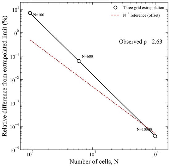
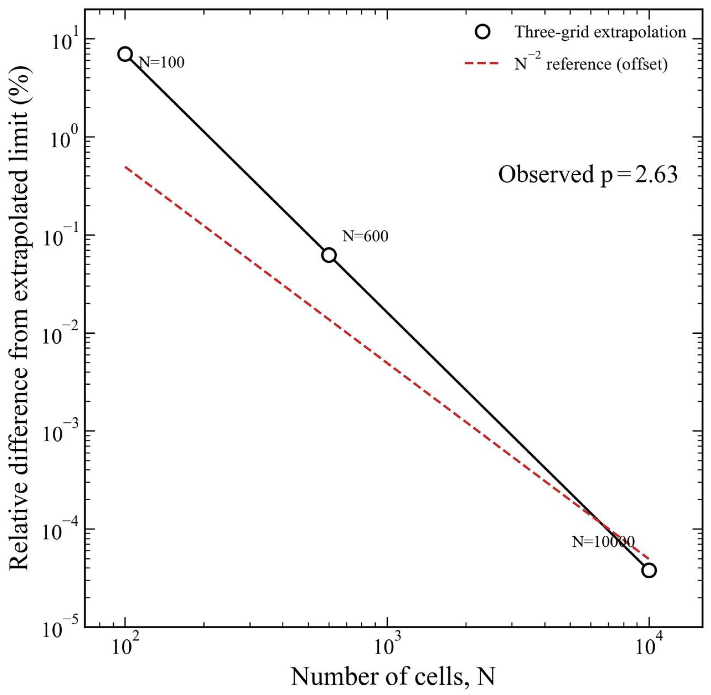
As listed in Table 3, refinement from 600 to 10,000 cells changes the tested outlet’s superficial velocity by 0.0623% compared with 6.9202% between 100 and 600 cells. The 600-cell grid, with Δz = 10 m, is retained on this basis for the tested outlet transport quantity. This comparison does not establish grid independence of the axial gas-holdup, pressure, or velocity fields or of the local injection source response. Equation (37) preserves the integrated gas mass input when the injection cell width changes; this source normalization is distinct from spatial convergence of the surrounding field.

Table 3. Axial-grid comparison for the reference configuration.

Cells N	Δz (m)	jl,out (m/s)	Change from Preceding Grid (%)
100	60	4.479	—
600	10	4.812	6.9202
10,000	0.6	4.815	0.0623

To describe the refinement trend, the three values are fitted with j(N) = j∞ + C N^(−p). The unequal refinement ratios, 6 and 16.6667, are included explicitly when solving for the observed order:

$${\displaystyle \frac{4.812-4.479}{4.815-4.812}}={\displaystyle \frac{{100}^{-p}-{600}^{-p}}{{600}^{-p}-{\mathrm{10,000}}^{-p}}}, p\simeq 2.63.$$

(41)

The double-logarithmic presentation in Figure 2 uses EN = 100|j(N) − j∞|/|j∞|. Its slope describes the observed convergence of this outlet quantity. The value p ≈ 2.63 is a three-grid result for the reported scalar, while the successive grid differences quantify the practical sensitivity used to select N. The observed order applies to this outlet scalar; the spatial and transient fields are interpreted at the reported resolution.

Figure 2. Grid convergence of the outlet slurry superficial velocity.

4.2. Time-Step Sensitivity

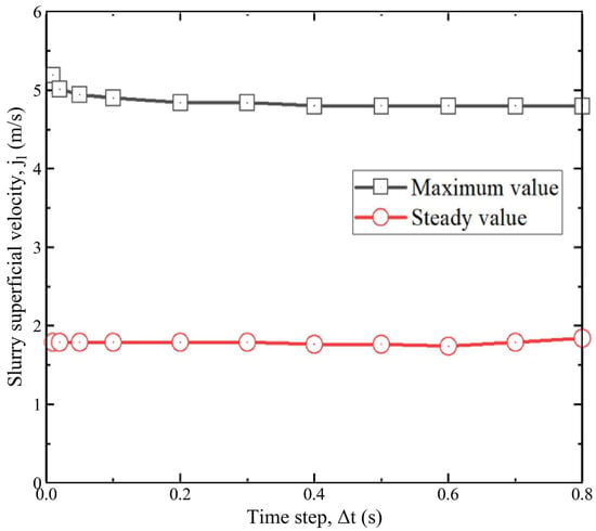
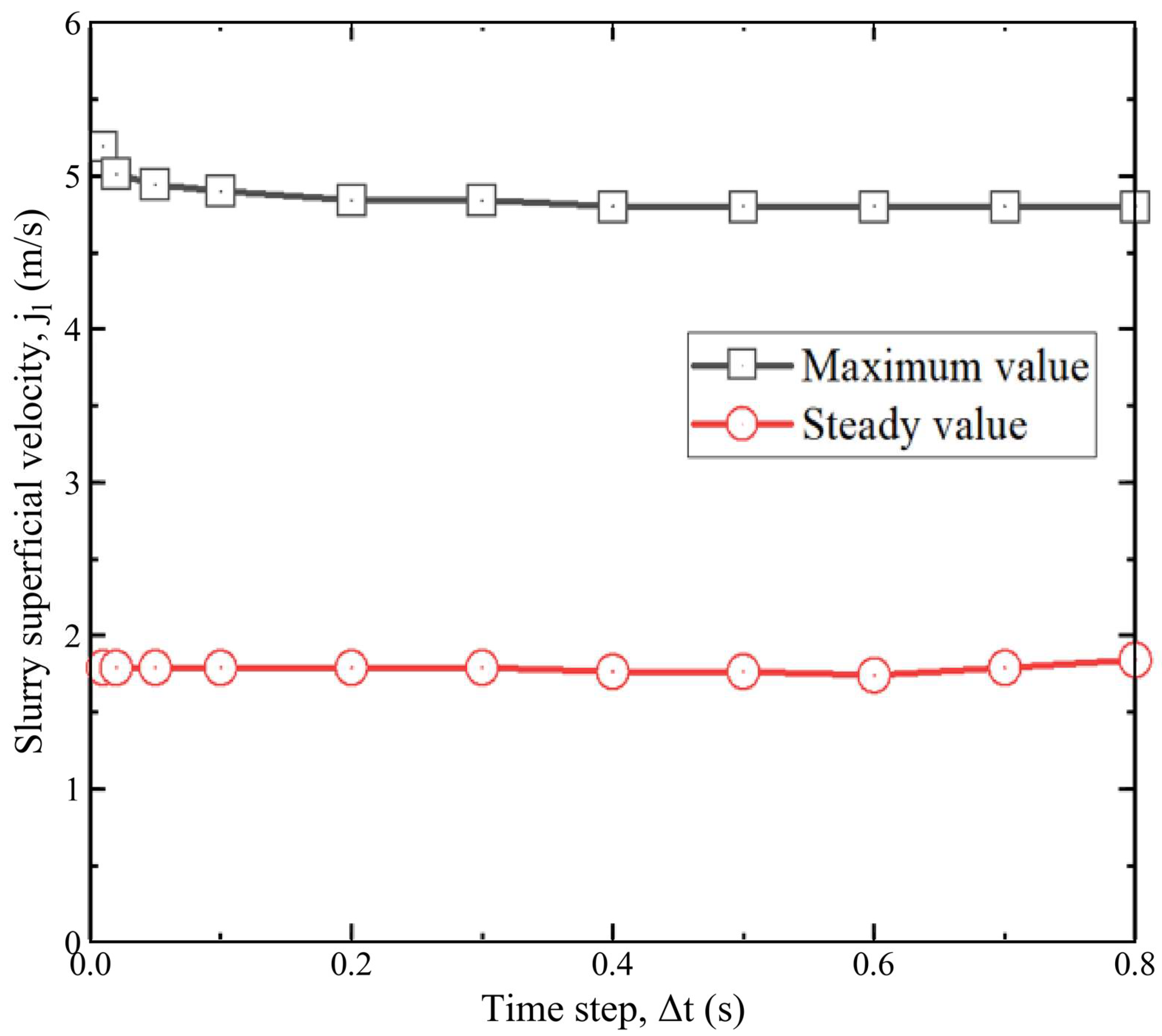
The time-step comparison uses the selected 600-cell grid and reports two distinct quantities: the maximum outlet superficial velocity during start-up and the steady outlet superficial velocity. The steady velocity remains close to 1.8 m/s, whereas the resolved transient maximum rises from approximately 4.8 to 5.2 m/s as the time step decreases. The steady transport rate and the start-up peak therefore have different sensitivities to temporal resolution.

This trend is consistent with the numerical damping of the first-order backward-Euler method. For an oscillatory mode with angular frequency ω, the amplification factor magnitude is

$$\left|G\right|={\left[1+{\left(\omega \Delta t\right)}^2\right]}^{-1/2}.$$

(42)

A larger time step damps this oscillatory mode more strongly, whereas reducing Δt decreases its artificial attenuation. The role of backward-Euler dissipation is also discussed for compressible two-fluid pipe calculations by Sanderse et al. [37]. This provides numerical context for the observed increase in the resolved start-up peak, rather than a convergence test of the present transient fields. At steady state, the temporal derivative vanishes, consistent with the weaker time-step sensitivity of the steady transport rate (Table 4).

Table 4. Steady outlet superficial velocity in the time-step assessment.

Δt (s)	Steady jl,out (m/s)	Change Relative to the 0.6 s Result (%)
0.6	1.74	—
0.4	1.77	1.7
0.2	1.79	2.8

The percentage difference uses the velocity at the smaller time step as its denominator. Velocities are rounded to two decimal places.

The differences between the Δt = 0.6 s result and the 0.4 and 0.2 s steady results are 1.7% and 2.8%, respectively, using the smaller step value as the reference. The calculations retain Δt = 0.6 s for the lifting performance comparisons. The start-up maximum in Figure 3 changes from approximately 4.8 to 5.2 m/s over the tested time steps, a spread of about 0.4 m/s or 7.7% relative to the finer step peak. This spread describes the observed peak sensitivity and is not a formal error bound. The selected time step introduces numerical damping of the transient response. Accordingly, the transient figures are interpreted as evolution at Δt = 0.6 s: they illustrate the sequence of gas propagation, material replacement, and outlet acceleration, while the precise peak amplitudes, occurrence times, and internal pressure or gas-holdup fluctuations are not claimed to be time-step independent.

Figure 3. Time-step sensitivity of the maximum and steady outlet superficial velocities.

4.3. Verification of Single-Phase Power-Law Flow

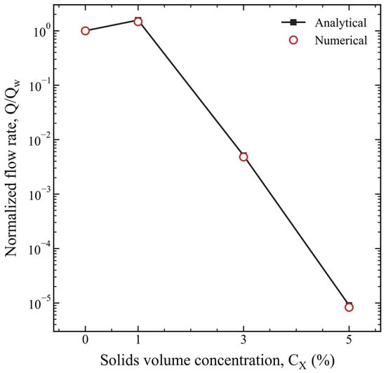
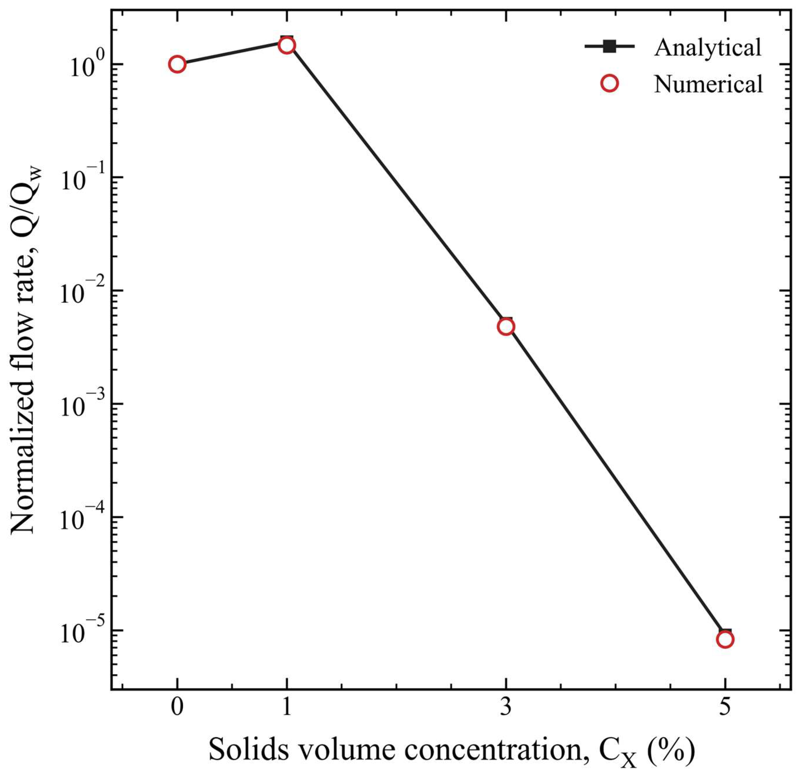
The single-phase benchmark compares seawater with 1%, 3%, and 5% rare earth slurry at the common wall shear stress τw = 1 Pa. These suspensions have power law indices n = 0.49514, 0.31179, and 0.20516, respectively, and explicitly test shear-thinning behavior. For steady, fully developed laminar flow in a circular pipe, the shear-stress magnitude is τ(r) = τw r/R. Integration of the power law relationship with no slip at r = R gives

$$u\left(r\right)={\displaystyle \frac{nR}{n+1}}{\left({\displaystyle \frac{{\tau }_w}{K}}\right)}^{1/n}\left[1-{\left({\displaystyle \frac{r}{R}}\right)}^{\left(n+1\right)/n}\right].$$

(43)

$$Q_{\mathrm{e}\mathrm{x}\mathrm{a}\mathrm{c}\mathrm{t}}={\displaystyle \frac{\pi R^{3}n}{3n+1}}{\left({\displaystyle \frac{{\tau }_w}{K}}\right)}^{1/n}, {\tau }_w={\displaystyle \frac{R\Delta p_f}{2L}}.$$

(44)

Here, R and L are the common pipe radius and length in meters and Δpf is the frictional pressure drop in pascals, with the hydrostatic contribution excluded. Q is the volumetric discharge in m³/s. The normalization q = Q/Qw uses the seawater discharge for the same geometry and wall stress, with μw = 1.3 × 10⁻³ Pa·s. It removes the common geometric factor πR³ and expresses the benchmark directly through the imposed stress and material properties:

$$q_{\mathrm{e}\mathrm{x}\mathrm{a}\mathrm{c}\mathrm{t}}={\displaystyle \frac{4n{\mu }_w}{\left(3n+1\right){\tau }_w}}{\left({\displaystyle \frac{{\tau }_w}{K}}\right)}^{1/n}, E_q=100{\displaystyle \frac{\left|q_{\mathrm{n}\mathrm{u}\mathrm{m}}-q_{\mathrm{e}\mathrm{x}\mathrm{a}\mathrm{c}\mathrm{t}}\right|}{\left|q_{\mathrm{e}\mathrm{x}\mathrm{a}\mathrm{c}\mathrm{t}}\right|}} \left(\mathrm{\%}\right).$$

(45)

q = Q/Qw is dimensionless. Seawater supplies the normalization; relative errors are evaluated for the three slurry cases.

As listed in Table 5, the numerical discharge of the 3% slurry is qnum = 0.0048. Relative errors for the 1%, 3%, and 5% cases are 6.21%, 6.12%, and 8.39%. Figure 4 displays the full discharge range on a logarithmic ordinate. The laminar reference corresponds to the Darcy wall friction relationship fD = 64/ReMR, equivalently fF = 16/ReMR in the Fanning convention. This is numerical verification of the selected single-phase power law response against an exact laminar solution. It is distinct from experimental constitutive validation and from validation of gas lifting of a non-Newtonian suspension. The subsequent air–water comparisons assess Newtonian gas–liquid discharge.

Table 5. Single-phase power law discharge comparison at τw = 1 Pa.

Liquid	K (Pa·sn)	n	qexact	qnum	Eq (%)
Seawater	0.0013	1	1	1	—
1% slurry	0.02664	0.49514	1.5673	1.47	6.21
3% slurry	0.56894	0.31179	0.005113	0.0048	6.12
5% slurry	2.41068	0.20516	9.06 × 10−6	8.30 × 10−6	8.39

Figure 4. Analytical and numerical normalized single-phase discharge for seawater and slurry at τw = 1 Pa.

4.4. Validation Against Air–Water Experiments

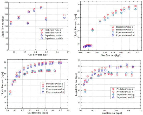
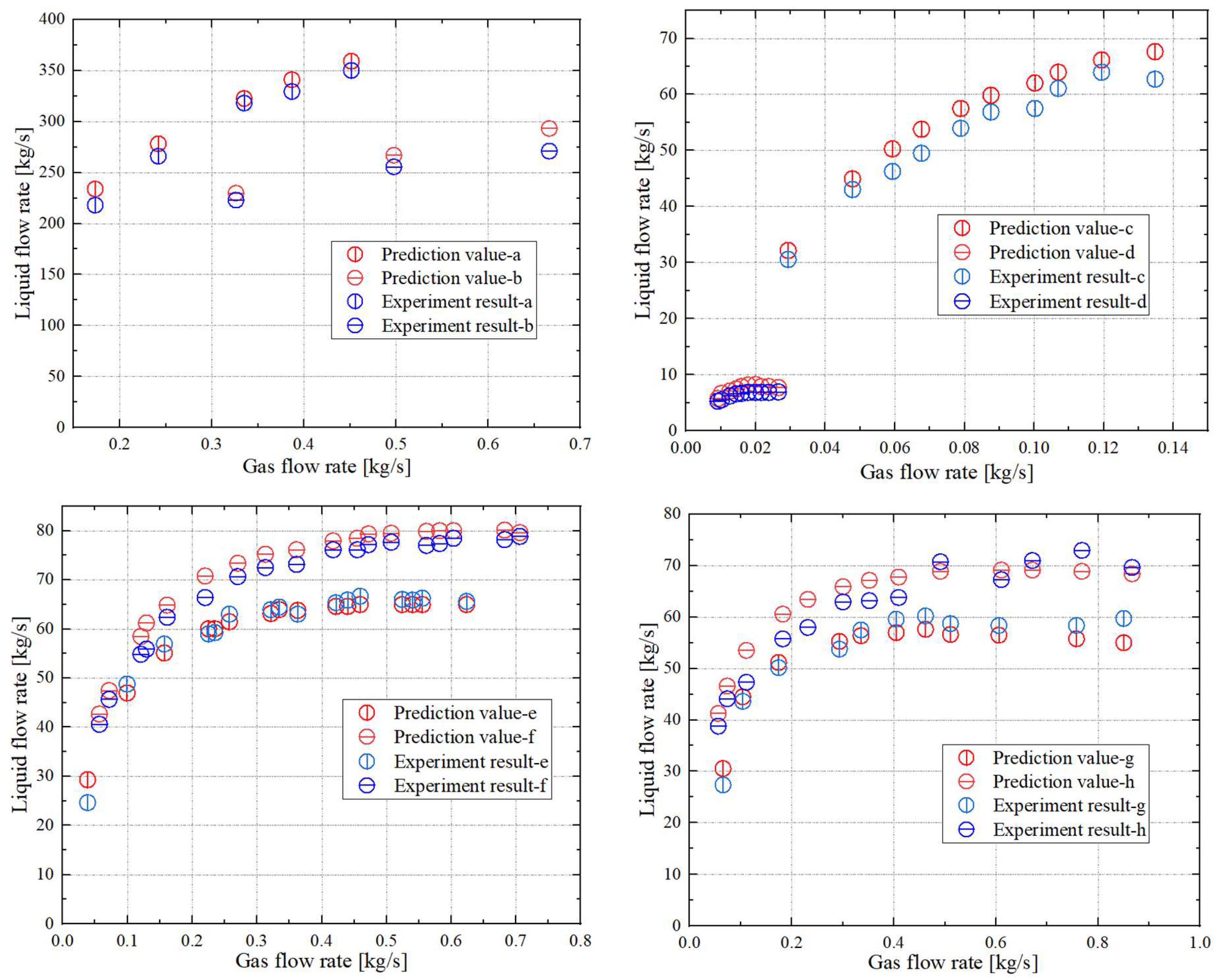
The experimental comparisons cover eight airlift configurations from Weber and Dedegil [38], Usami et al. [39], and Saito et al. [40,41], with the source datasets identified below and cross-referenced to the compilation in [33]. The selected experiments use air and particle-free water, including freshwater and seawater, so CX = 0, and the liquid is Newtonian (n = 1). The comparison spans numerical pipe diameters of 0.0757–0.300 m, representing pipe lengths of 12.48–451 m and injection depths of 8.15–125 m. Injection depth is measured downward from the external free surface to the gas inlet. The numerical wall specifications are ε/D = 0 for cases a–f and ε/D = 4.2 × 10⁻⁴ for g and h; these values describe the model inputs, rather than new measurements of experimental pipe roughness.

The selected liquids are particle-free freshwater or seawater, with zero solids loading. Gas input and liquid discharge are expressed as mass flow rates in kg/s. Each numerical–experimental pair is evaluated at the same gas mass input.

The experimental subsets in Figure 5 are identified by the original water lifting operation and its published data location. Cases a and b are the Weber–Dedegil water-lifting datasets [38], identified as W1 and W2 in Table 2 of Hatakeyama et al. [33] and reproduced as experimental points in Figure 6 and Figure 7 of that paper, respectively.

Figure 5. Comparison of numerical and experimental liquid mass discharge in eight air–water configurations.

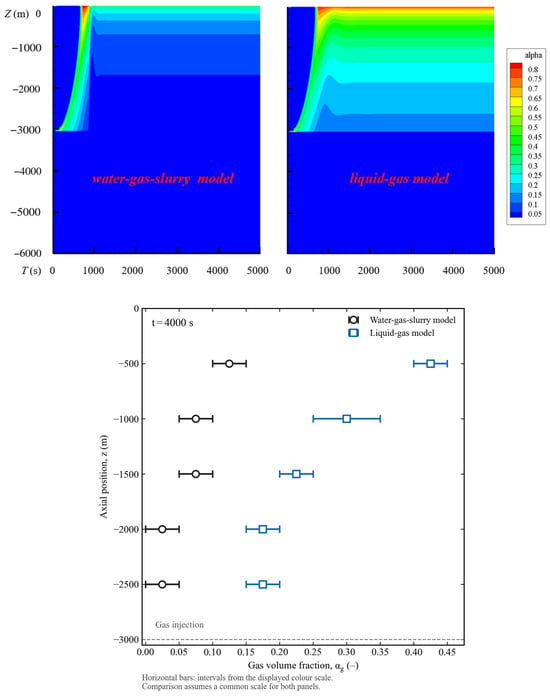
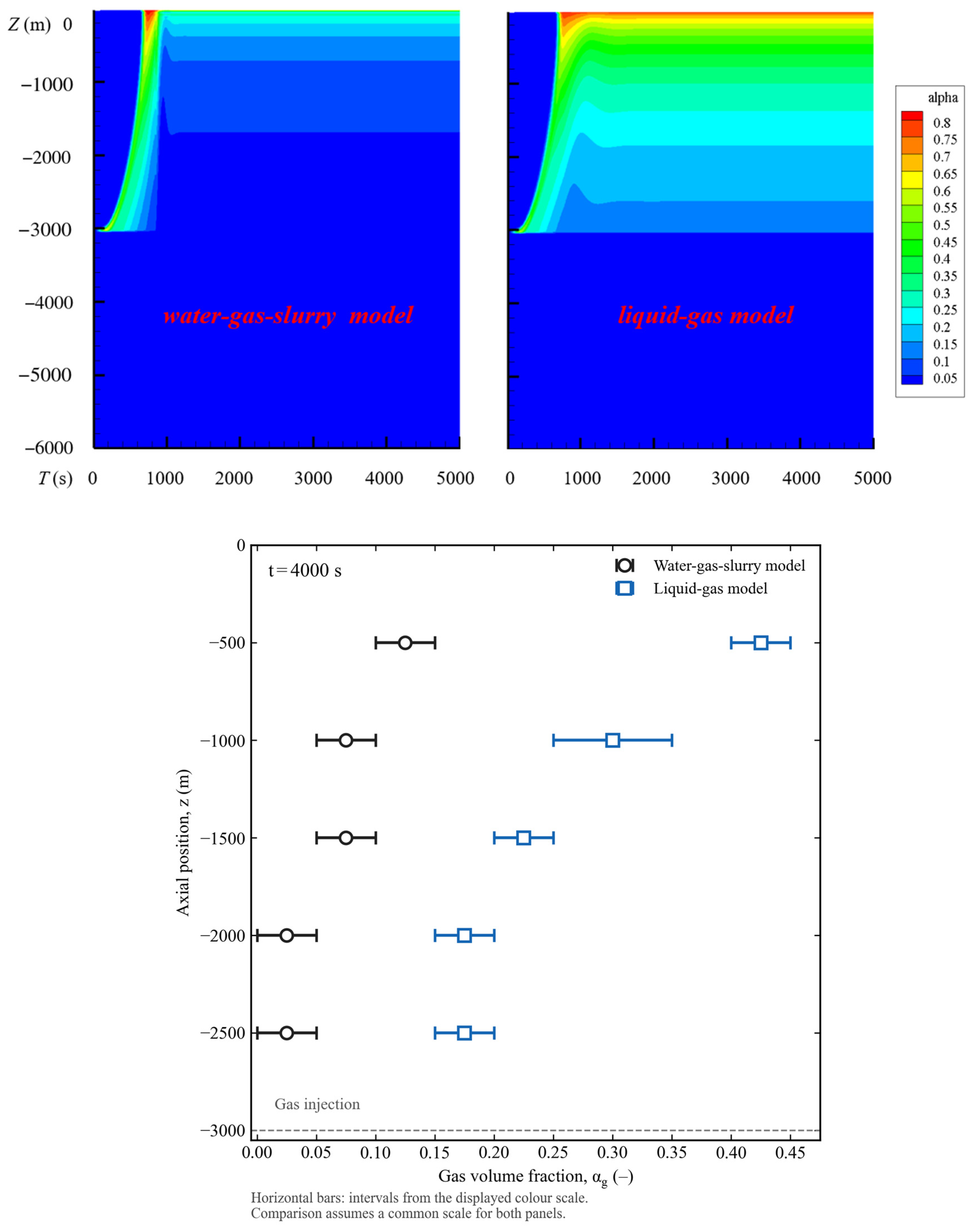
Figure 6. Gas-holdup sensitivity to liquid property treatment, with evolution above and approximate color-scale comparison at t = 4000 s below.

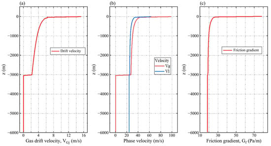
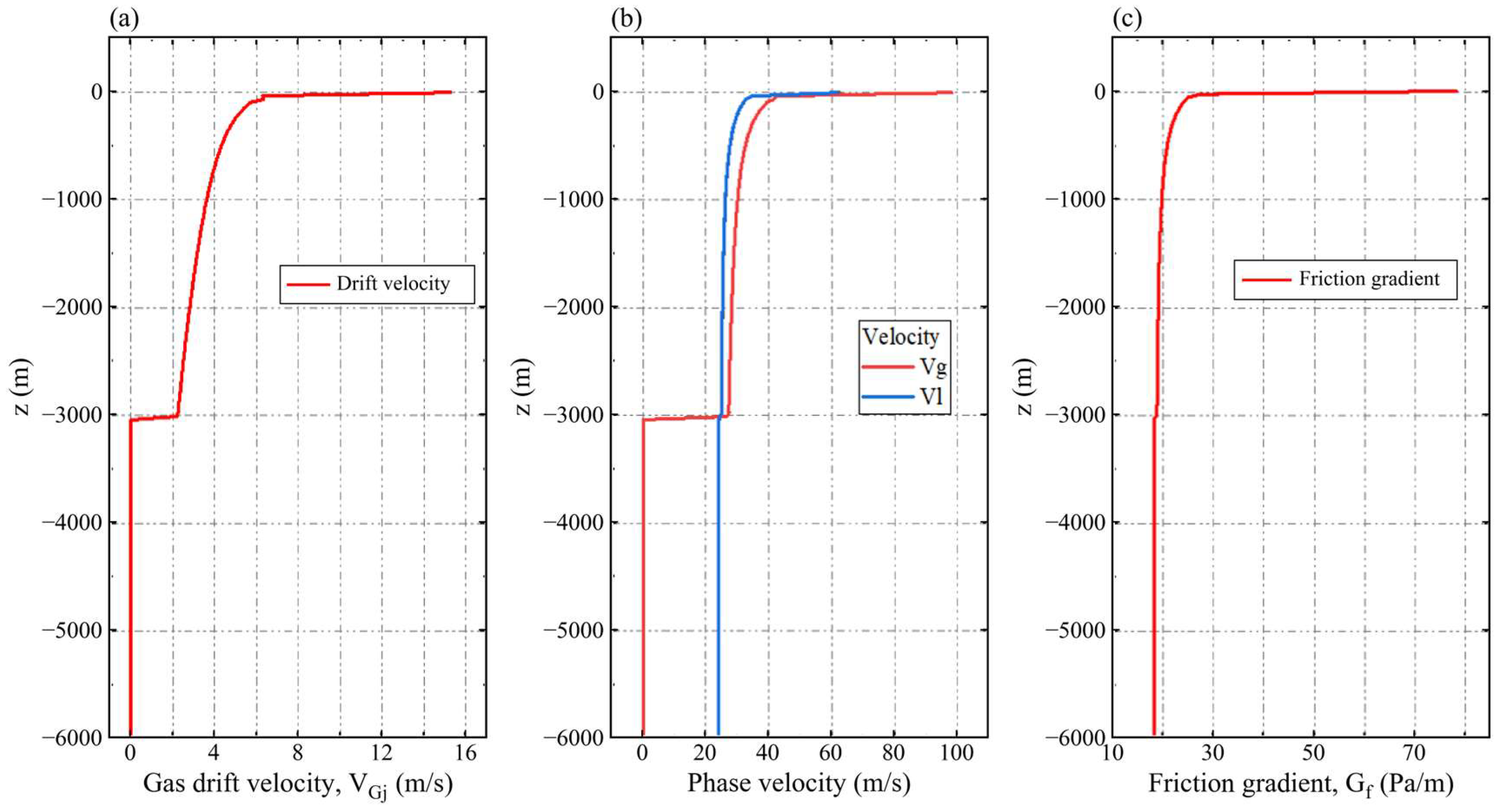
Figure 7. Late-time axial profiles of gas drift velocity (a), phase velocities (b), and wall-friction pressure gradient (c).

Cases c and d use Fig. 6 of Usami et al. [39] (p. 31, Section 4.1 on gas–liquid two-phase flow): c is the lower-injection seawater series for the 155.4 mm pipe and d is the indoor pure-water series for the 75.7 mm pipe. These are distinct from the solid transport experiments in Section 4.2. Table 6 follows the c/d labels in Figure 5; the adopted numerical diameter for c is rounded to 0.155 m. Its represented straight pipe length of 37.59 m follows the segment lengths in Table 2 of [33], rather than the 37.84 m complete apparatus length reported in [39].

Table 6. Air–water reference configurations and recalculated discharge deviations.

Case/Reference	D (m)	L (m)	hinj (m)	ε/D	Pairs	MARD (%)	MRD (%)
a/[33,38]	0.300	138	125	0	5	3.89	+3.89
b/[33,38]	0.300	451	102	0	3	5.23	+5.23
c/[39]	0.155	37.59	26.87	0	10	6.28	+6.28
d/[39]	0.0757	12.48	8.15	0	10	15.88	+15.88
e/[33,40]	0.151	212.6	71	0	16	2.90	+0.03
f/[40]	0.151	212.6	100	0	18	3.92	+3.92
g/[41]	0.151	212.6	71	4.2 × 10−4	11	4.39	−1.02
h/[41]	0.151	212.6	100	4.2 × 10−4	13	5.83	+3.89
All a–h	—	—	—	—	86	5.79	+4.27

The reported inputs for cases e and f correspond to the 6 in (71) and 6 in (100) configurations listed in Table 1 of Saito et al. [40]. Their water-only operation is described in Section 4.3 and represented in Fig. 8 of [40], which plots liquid holdup against gas Froude number. The 71 m water discharge configuration is also reproduced as S4 in Fig. 5 of Hatakeyama et al. [33]. These locators distinguish the water-only operating conditions from the solid transport data in Section 4.4 of [40].

Cases g and h use the 151 mm water-pumping series in Fig. 7 of Saito et al. [41], with injection depths of 71 and 100 m, respectively. Their gas-containing lengths are 83.6 and 112.6 m, and the corresponding submergence ratios are 0.849 and 0.888. The apparatus uses tap water and compressed air. Accordingly, all selected validation subsets have zero solids loading, even where the source paper also discusses solid transportation or a different application.

The numerical gas input is matched to each experimental comparison point. The temperature is prescribed as 293.15 K, the air gas constant is 287 J/(kg·K), and the absolute atmospheric reference is 101,325 Pa. Gas is introduced at the specified injection level and increased linearly over 60 s to its target mass flow. This ramp sets the numerical start-up history; the experimental comparison concerns the resulting stationary discharge. Table 7 summarizes these numerical operating definitions.

Table 7. Numerical operating definitions used in the airlift comparisons.

Quantity	Setting or Definition
Liquid	Water; Newtonian, n = 1; CX = 0
Gas feed specification	Mass flow matched to each experimental abscissa in the comparison figure
Gas injection history	ṁg(t) = ṁg,max min(1, t/60 s)
Temperature	T = 293.15 K
Air gas constant	Rg = 287 J/(kg·K)
Atmospheric reference	patm = 101,325 Pa, absolute
Full-domain inlet	pin = patm + ρout g Hs
Injection-level inlet	pin = patm + ρout g hinj − Gf,suc Lsuc
Outlet	pout = patm exp[−g Hout/(Rg T)]

The inlet expression is selected for the represented computational domain. Hs is submerged length; Lsuc is suction section length; Gf,suc is its frictional pressure gradient; Hout is outlet elevation above the external free surface.

The inlet pressure is set by the external hydrostatic head. When the computational domain begins at the injection level, the suction section friction loss is included in the inlet pressure. The outlet pressure is atmospheric pressure corrected for outlet elevation. These hydraulic boundaries determine operating pressure together with the internal momentum balance; a separate compressor discharge pressure is not prescribed.

The mean absolute relative deviation (MARD) quantifies the magnitude of the discharge discrepancy, while the mean relative deviation (MRD) retains its sign. With Np paired samples and liquid mass discharges ṁl,num,i and ṁl,exp,i at equal gas inputs,

$$\mathrm{M}\mathrm{A}\mathrm{R}\mathrm{D}={\displaystyle \frac{100}{N_p}}{\displaystyle \sum _{i=1}^{N_p}}\left|{\displaystyle \frac{{\dot{m}}_{l,\mathrm{n}\mathrm{u}\mathrm{m},i}-{\dot{m}}_{l,\mathrm{e}\mathrm{x}\mathrm{p},i}}{{\dot{m}}_{l,\mathrm{e}\mathrm{x}\mathrm{p},i}}}\right| \left(\mathrm{\%}\right).$$

(46)

$$\mathrm{M}\mathrm{R}\mathrm{D}={\displaystyle \frac{100}{N_p}}{\displaystyle \sum _{i=1}^{N_p}}{\displaystyle \frac{{\dot{m}}_{l,\mathrm{n}\mathrm{u}\mathrm{m},i}-{\dot{m}}_{l,\mathrm{e}\mathrm{x}\mathrm{p},i}}{{\dot{m}}_{l,\mathrm{e}\mathrm{x}\mathrm{p},i}}} \left(\mathrm{\%}\right).$$

(47)

Positive MRD denotes average overprediction and negative MRD average underprediction. Pooling all 86 pointwise deviations gives MARD = 5.79% and MRD = +4.27%; every pair receives equal weight. These pooled statistics are distinct from an unweighted average of the eight group percentages. Individual group MARD ranges from 2.90% to 15.88%, with the largest discrepancy in smooth case d. Rough pipe cases g and h give 4.39% and 5.83%, respectively, so pipe roughness alone does not order the observed deviations.

The earlier void-fraction-correlated drift flux framework was assessed against apparent velocities, gas volume fractions, and outlet pressure drop by Liu [29]. That evidence concerns the formulation and operating conditions examined in the earlier work and supports the background of the present model. The current eight air–water comparisons evaluate liquid mass discharge for the selected Newtonian configurations.

The analytical benchmark verifies the gas-free, single-phase power law response. Published mud correlations [15,16] provide the material property basis for K and n, while the air–water comparisons assess the combined hydraulic prediction rather than each closure separately. Independent experimental validation of the coupled non-Newtonian slurry-lifting treatment is not included. Section 5 therefore presents model predictions and parameter sensitivity under the stated closures and operating conditions. The air–water discharge deviations are not assigned as error estimates to the deep-sea slurry calculations.

4.5. Liquid Continuity Check

The supplementary check uses L = 6000 m, D = 0.20 m, a smooth pipe, 4 m outlet elevation above the external water level, injection depth 3000 m, gas mass input 10 kg/s reached through a 60 s linear ramp, and T = 293.15 K. Liquid properties are prescribed as ρl = 1020 kg/m³, K = 13.2589 Pa·sⁿ, and n = 0.0336, with N = 600 axial cells. The calculation is advanced from the initial state to t = 1000 s using the numerical controls in Section 3.2.

At t = 1000 s, A = πD²/4 = 0.03141593 m². At the physical outlet, αg = 0.77261582 and vl = 96.807937 m/s give Qout = A(1 − αg)vl = 0.69154602 m³/s. At z = −3996 m below injection, αg = 0 and vl = 22.012483 m/s give Qbelow = Avl = 0.69154255 m³/s. Their relative difference, 100|Qout − Qbelow|/Qout, is 0.000502%. The liquid fraction is applied once to the intrinsic outlet liquid velocity; jl = (1 − αg)vl is the superficial velocity.

The finite-volume liquid inventory is Ml = Σρl(1 − αg)AΔz. Including its time change gives Rl = ṁl,in − ṁl,out − (Ml,k − Ml,k−1)/Δt. At the same endpoint, the inventory change rate is −0.003250 kg/s, and the absolute residual is 0.000292 kg/s, or 0.000041% of max(|ṁl,in|, |ṁl,out|). This independently checks the cross-sectional flux definition and its consistency with liquid continuity.

For this check, a stationary monitoring window is defined by CVW < 0.1% and δ12 < 0.1% for outlet discharge and the interior pressure and gas fraction at z = −1501 m. Over 940 < t ≤ 1000 s (101 samples), their CVW values are 0.000341%, 0.000060%, and 0.002083%, respectively. Comparing 940 < t ≤ 970 s with 970 < t ≤ 1000 s gives δ12 = 0.000595%, 0.000048%, and 0.003289%, using the later mean as the denominator. These values satisfy the stated monitoring criteria for this supplementary case.

5. Results and Discussion

5.1. Material Replacement, Gas-Holdup Evolution, and Outlet Response

Section 4 assesses the single-phase power law response analytically and gas–liquid lifting discharge experimentally. The 86 paired air–water samples give pooled MARD = 5.79% and MRD = +4.27%. The following 6000 m slurry calculations examine model-predicted macroscopic transport at the reported spatial and temporal resolution. First, two liquid property treatments are compared under common geometry and gas input to assess the sensitivity of gas-holdup evolution to the representation of initial water and incoming slurry. Both treatments use D = 0.20 m, L = 6000 m, hinj = 3000 m, final gas input 10 kg/s, and incoming slurry concentration CX = 0.10. In the upper panels of Figure 6, the water–gas–slurry and liquid–gas results appear on the left and right, respectively.

The water–gas–slurry formulation treats external seawater as the hydrostatic environment and resolves gas and an averaged liquid suspension inside of the pipe. Incoming slurry replaces the water initially present in the submerged pipe through accumulated inflow accounting and material property assignment, with occupied fraction weighting in partially replaced cells. The slurry density and constitutive parameters follow its prescribed solids concentration. The carrier water and particles share liquid velocity. The occupied fraction specifies how the initial water and suspension properties contribute to a cell’s density and wall resistance during replacement. The liquid–gas reference applies the same slurry property treatment throughout the pipe. The comparison therefore examines model sensitivity to the representation of changing liquid properties during start-up.

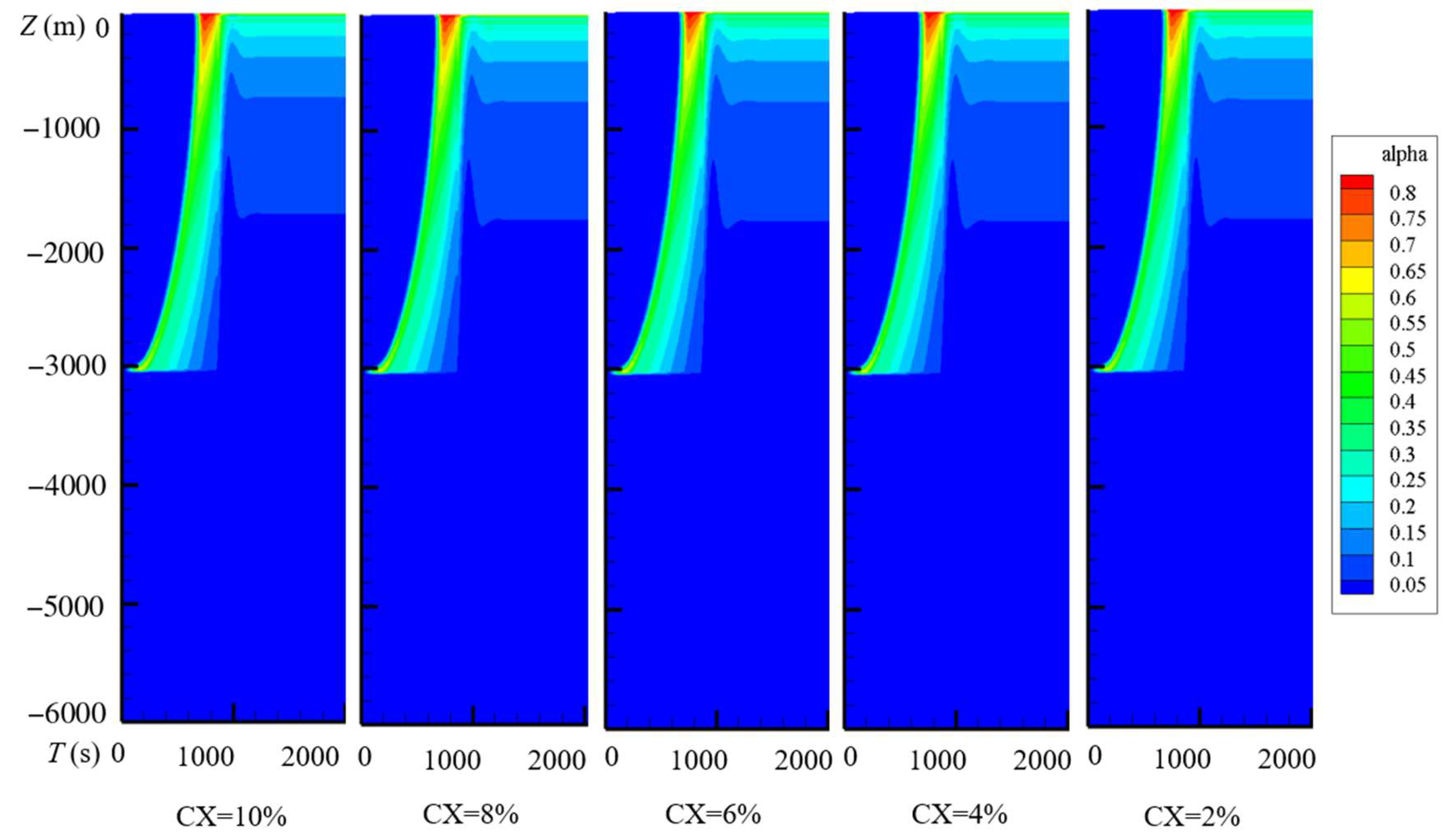
During start-up, gas accumulates near the injection point, and an elevated cross-sectionally averaged gas fraction αg propagates upward. This dimensionless fraction measures the local gas volume relative to the gas–liquid mixture volume. Decreasing pressure permits gas expansion, changing gas holdup, phase velocities, and driving head and producing a predicted transient outlet acceleration. The initial excursion subsequently subsides while gas injection continues, and the flow approaches the late-time operating stage. The contour maps in Figure 6 and in the three parameter series below use a displayed gas fraction range of 0–0.8 over −6000 ≤ z ≤ 0 m, with time windows of 0–5000 s for Figure 6, 0–2000 s for the concentration series, and 0–3000 s for the other two series. All use the initial liquid inventory, pressure boundaries, and 60 s gas ramp specified in Section 3.1.

At t = 4000 s and z = −500 m, the water–gas–slurry and liquid–gas predictions have approximate gas-holdup intervals of 0.10–0.15 and 0.40–0.45, respectively; at z = −1500 m, they are 0.05–0.10 and 0.20–0.25. Their approximate axial means over −3000 ≤ z ≤ −100 m are 0.045–0.095 and 0.246–0.296. This interval excludes the terminal outlet band, and Equation (48) defines the axial mean. These intervals are estimates from the color scale and support a semi-quantitative comparison. The difference demonstrates sensitivity to liquid property treatment; it does not establish the accuracy or superiority of either prediction.

The profiles at t = 4000 s in Figure 6 are late-time snapshots following the dominant start-up evolution. The parameter series field plots are likewise described as a late-time operating stage. Equation (49) defines the window coefficient of variation and the change between consecutive means used for the separately prescribed outlet diagnostic below. Its reported outlet statistics apply to that diagnostic and are distinct from the interpretation of Figure 6 and the parameter series histories. Physical temporal variation is distinguished from convergence of the inner pressure–velocity iterations within one time step.

$${\overline{\alpha }}_{g,z}\left(t\right)={\displaystyle \frac{1}{z_2-z_1}}{\int }_{z_1}^{z_2}{\alpha }_g\left(z,t\right)\hspace{0.17em}\mathrm{d}z, z_1=-3000\hspace{0.17em}\mathrm{m}, z_2=-100\hspace{0.17em}\mathrm{m}.$$

(48)

$${\mathrm{C}\mathrm{V}}_W=100{\displaystyle \frac{{\sigma }_W}{\left|{\overline{X}}_W\right|}}, {\delta }_{12}=100{\displaystyle \frac{\left|{\overline{X}}_{W_2}-{\overline{X}}_{W_1}\right|}{\left|{\overline{X}}_{W_2}\right|}} \left(\mathrm{\%}\right).$$

(49)

Figure 7 uses the same conditions as Figure 6 and shows changes at injection and toward the outlet. The gas-free lower section carries suspension, while injected gas changes mixture density and relative motion above it. The total volumetric flux is j = αgvg + αlvl, with vg = C0j + vgj. The gas drift is VGj = vg − j = (C0 − 1)j + vgj = αl(vg − vl). Here, vgj is the dimensional intercept, vg − vl is phase-to-phase slip, and vm is mass-averaged mixture velocity; all velocities are in m/s.

The wall friction pressure gradient Gf = 4τw/D is in Pa/m, with wall shear τw in Pa. Its axial integral gives the frictional component of pressure loss; gravity and acceleration also contribute to the complete pressure balance. The pressure decrease toward the outlet causes gas expansion and an axial increase in phase velocity, while start-up outlet acceleration describes temporal evolution.

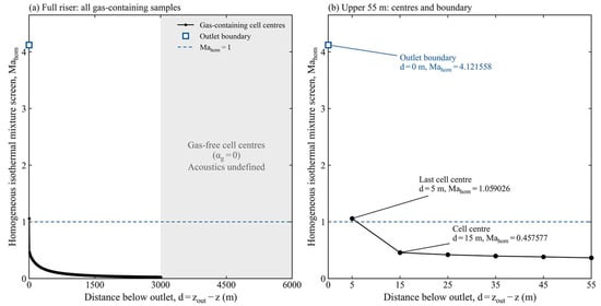
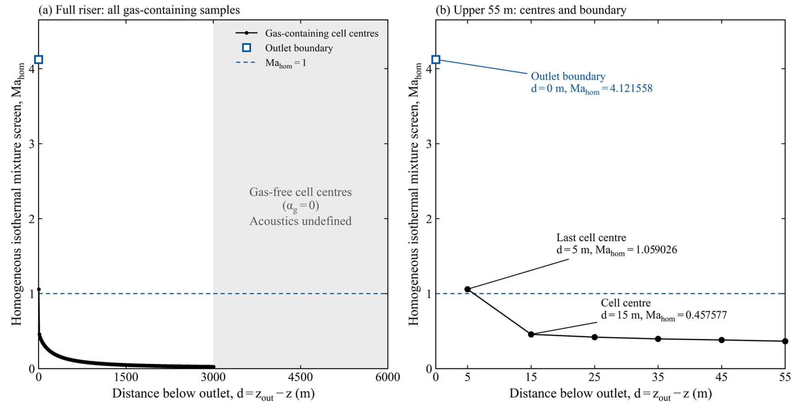
The additional outlet diagnostic prescribes N = 600 cells, Δt = 0.6 s, L = 6000 m, D = 0.20 m, a smooth pipe, hinj = 3000 m, gas input 10 kg/s, ρl = 1020 kg/m³, K = 13.2589 Pa·sⁿ, and n = 0.0336 independently of the concentration correlations. At t = 3000 s, the homogeneous isothermal mixture indicator [42] is Mh = |vm|√(αgρm/pabs) using absolute pressure and mass-averaged velocity. Distance d is measured upstream from the physical outlet (Figure 8 and Table 8).

Figure 8. Axial distribution of the homogeneous mixture Mach indicator and enlarged outlet region at t = 3000 s.

Table 8. Homogeneous isothermal mixture Mach indicator at t = 3000 s for the separately prescribed property diagnostic.

Location	Distance Upstream from Outlet d (m)	Mh (–)
Outlet boundary face	0	4.1216
Last interior center	5	1.0590
Next interior center	15	0.4576

Mh is 4.1216 at the outlet face (d = 0), 1.0590 at the final interior center (d = 5 m), and 0.4576 at the next center (d = 15 m). The remaining gas-containing interior centers have Mh ≤ 0.4576. The terminal region includes both samples above unity. The gas-free lower section is identified separately because finite liquid acoustics are outside of the incompressible liquid treatment.

The coupled drift flux characteristics provide a separate diagnostic: every gas-containing interior center retains an upstream-propagating mode, including −7.60 m/s at the last center. At the outlet face, the three local speeds, approximately 71.34, 129.60, and 329.26 m/s, point outward. This sign pattern changes between the final interior center and the outlet face, making the terminal control volume essential to the interpretation. The prescribed pressure outlet defines the scope of the calculated terminal acceleration. Targeted outlet pressure and phase discharge measurements can guide assessment of this mechanism and development of a characteristic-compatible critical flow treatment.

$$M_h={\displaystyle \frac{\left|v_m\right|}{c_h}}=\left|v_m\right|\sqrt{{\displaystyle \frac{{\alpha }_g{\rho }_m}{p_{\mathrm{a}\mathrm{b}\mathrm{s}}}}}, c_h^2={\displaystyle \frac{p_{\mathrm{a}\mathrm{b}\mathrm{s}}}{{\alpha }_g{\rho }_m}}.$$

(50)

The displayed positions retain both values above unity. The remaining gas-containing interior centers have Mh ≤ 0.4576. The diagnostic inputs are distinct from concentration-derived slurry properties.

For this diagnostic, Qout = ṁl,out/1020. Over 2400 < t ≤ 3000 s, 1000 equally spaced samples give mean Qout = 0.691548 m³/s, coefficient of variation 3.35 × 10⁻⁵%, and normalized peak-to-peak fluctuation 1.67 × 10⁻⁴%. The consecutive windows 2400 < t ≤ 2700 s and 2700 < t ≤ 3000 s contain 500 samples each; their means differ by 7.35 × 10⁻⁷%, normalized by the later mean. These statistics characterize its late-time outlet signal.

5.2. Concentration-Dependent Slurry Transport

The concentration series varies the incoming suspension’s solids volume fraction CX from 0.02 to 0.10 at fixed geometry and gas input. CX determines power law properties and suspension density and is distinct from gas fraction αg. With ρw = 1020 kg/m³ and particle density ρs = 2800 kg/m³, ρl = (1 − CX)ρw + CXρs gives 1055.6–1198.0 kg/m³. The constitutive response combines consistency K and index n through apparent viscosity μapp = K|$\dot{\mathsf{\gamma }}$|ⁿ⁻¹, so concentration changes the resistance evaluated at the local shear rate. Section 2.3 specifies the constitutive correlations and branch assignment; Table 9 lists the case parameters.

Table 9. Concentration-dependent suspension properties for the 6000 m riser.

Case	CX (%)	ρsl (kg/m3)	K (Pa·sn)	n (–)
2-a	10	1198.0	17.13381	0.17310
2-b	8	1162.4	9.11229	0.18588
2-c	6	1126.8	4.03765	0.19866
2-d	4	1091.2	1.28260	0.25363
2-e	2	1055.6	0.18149	0.38615

Common conditions: D = 0.20 m, hinj = 3000 m, and gas input 10 kg/s. CX is the solids volume fraction within the gas-free slurry; density 2800 kg/m³ refers to the mud particles.

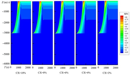
Figure 9 shows similar overall gas-holdup patterns, with an advancing start-up region followed by persistent axial color bands. Concentration nevertheless changes the constitutive response and suspension density entering the momentum balance. Gas holdup characterizes the fraction of the pipe occupied by gas, while resistance and discharge describe the hydraulic response of the suspension. The common pipe and injection configuration therefore produces similar macroscopic holdup patterns, accompanied by differences in resistance and discharge.

Figure 9. Gas-holdup evolution for slurry concentrations of 10%, 8%, 6%, 4%, and 2%, from left to right.

Slurry discharge is the cross-sectional flux Qsl = Aαlvl = Ajl, with A = πD²/4 and liquid superficial velocity jl. Below injection, αl = 1 and Qsl = Aul. Steady incompressible suspension continuity without distributed liquid sources gives the same discharge in the gas-free lower section and at the outlet; the lower-section plateau supplies the approximate profile-based comparisons. The representative liquid continuity check is reported in Section 4.5.

$$\begin{array}{c}{Q}_{\mathrm{s}\mathrm{l}}={\int }_{A_{\mathrm{o}\mathrm{u}\mathrm{t}}}{\alpha }_l{\mathbf{v}}_l\cdot \mathbf{n}\hspace{0.17em}\mathrm{d}A=A{\alpha }_{l,\mathrm{o}\mathrm{u}\mathrm{t}}{v}_{l,\mathrm{o}\mathrm{u}\mathrm{t}}=A{j}_{l,\mathrm{o}\mathrm{u}\mathrm{t}},\\ A={\displaystyle \frac{\pi D^2}{4}}.\end{array}$$

(51)

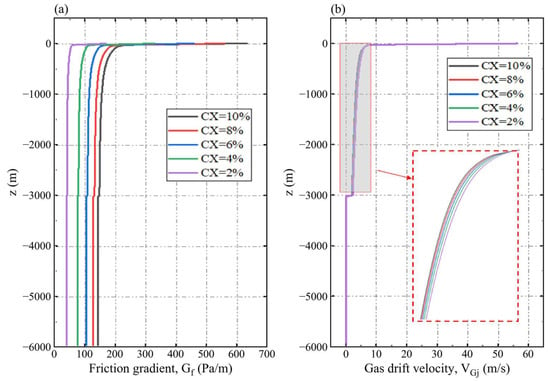
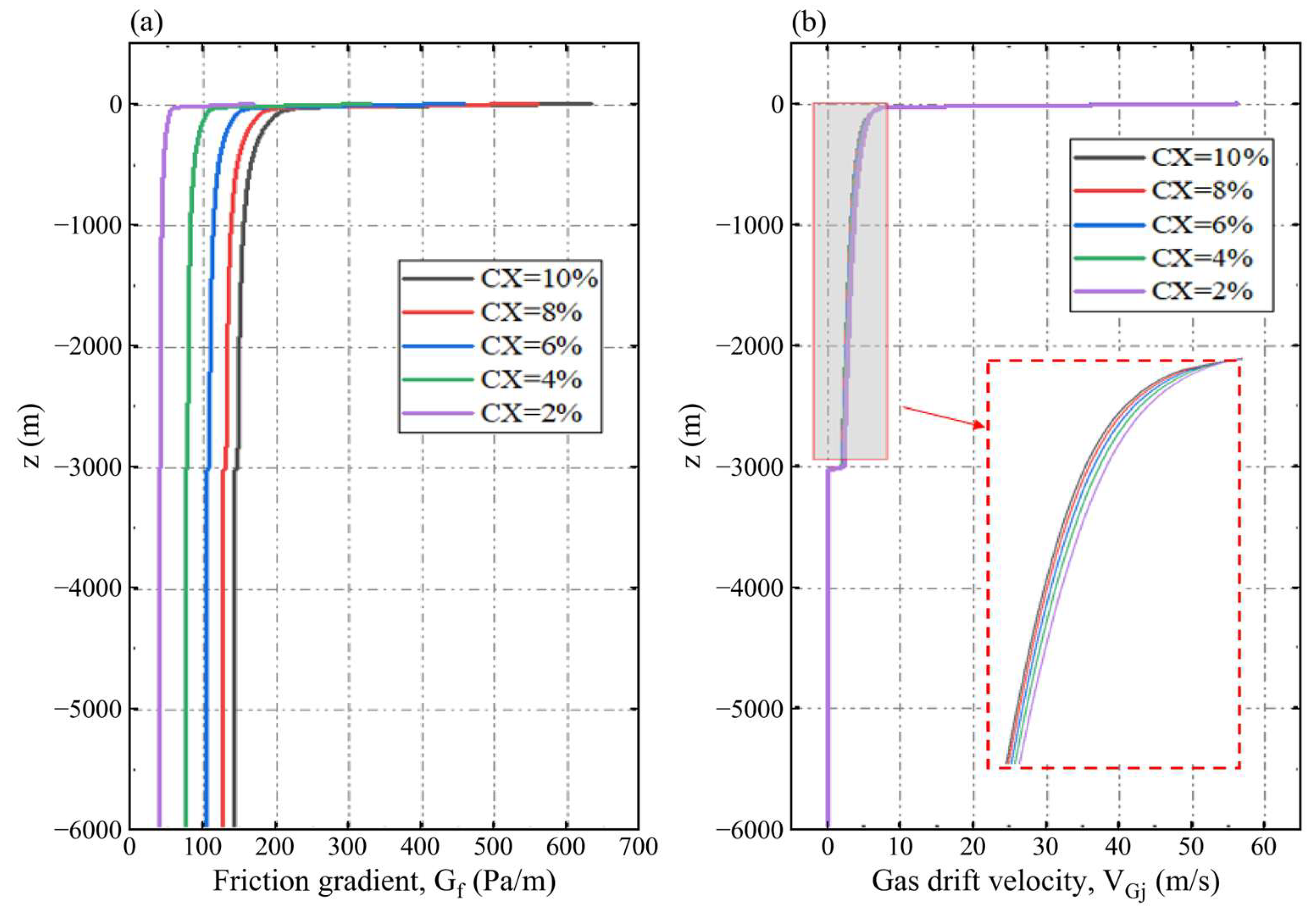
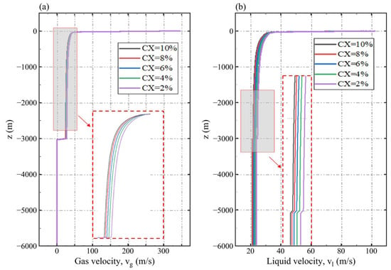
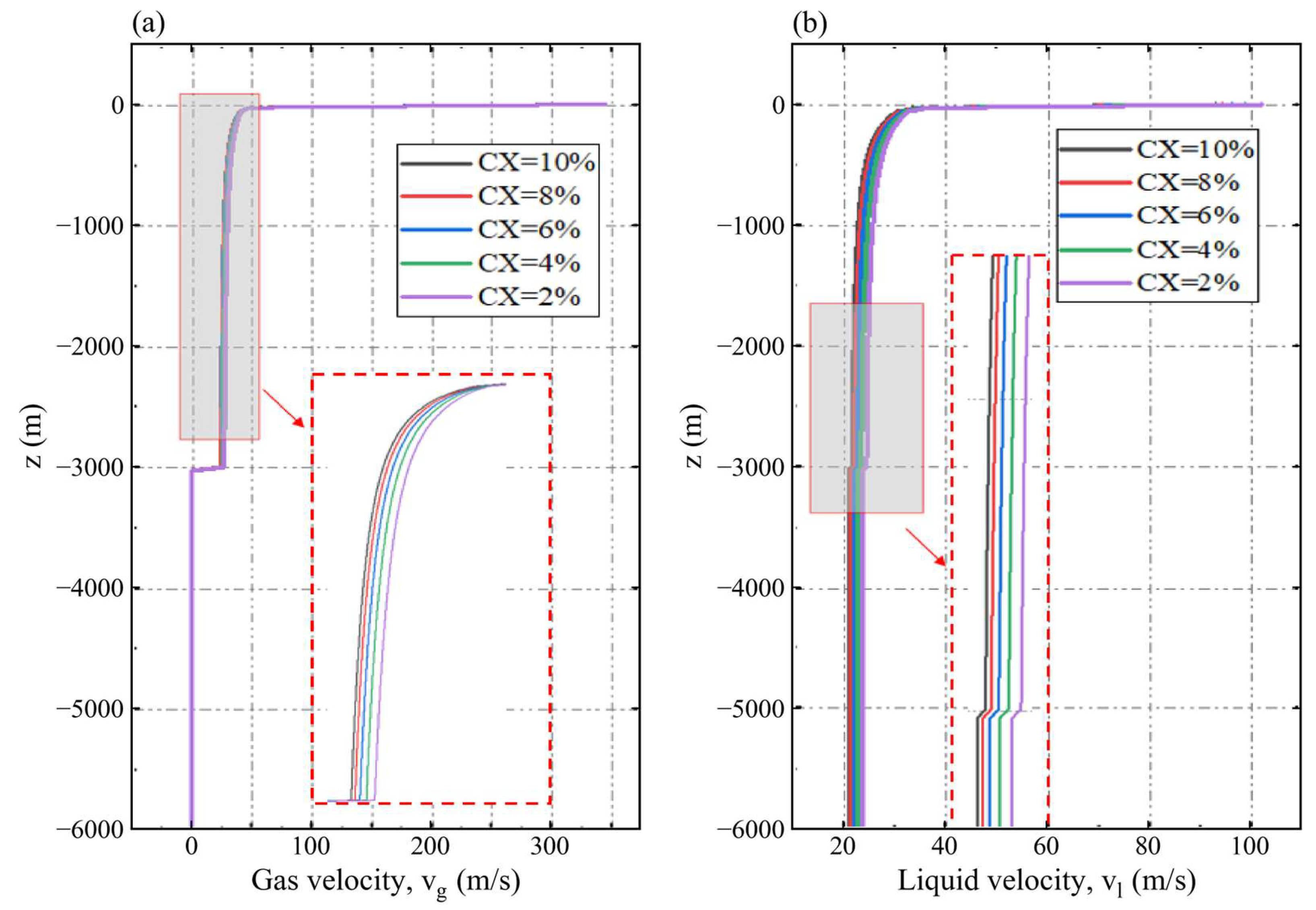
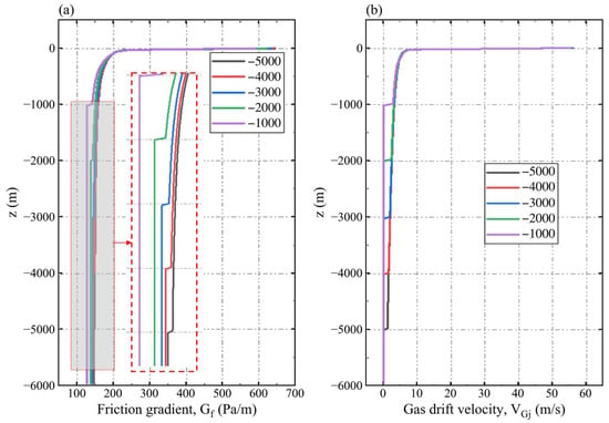
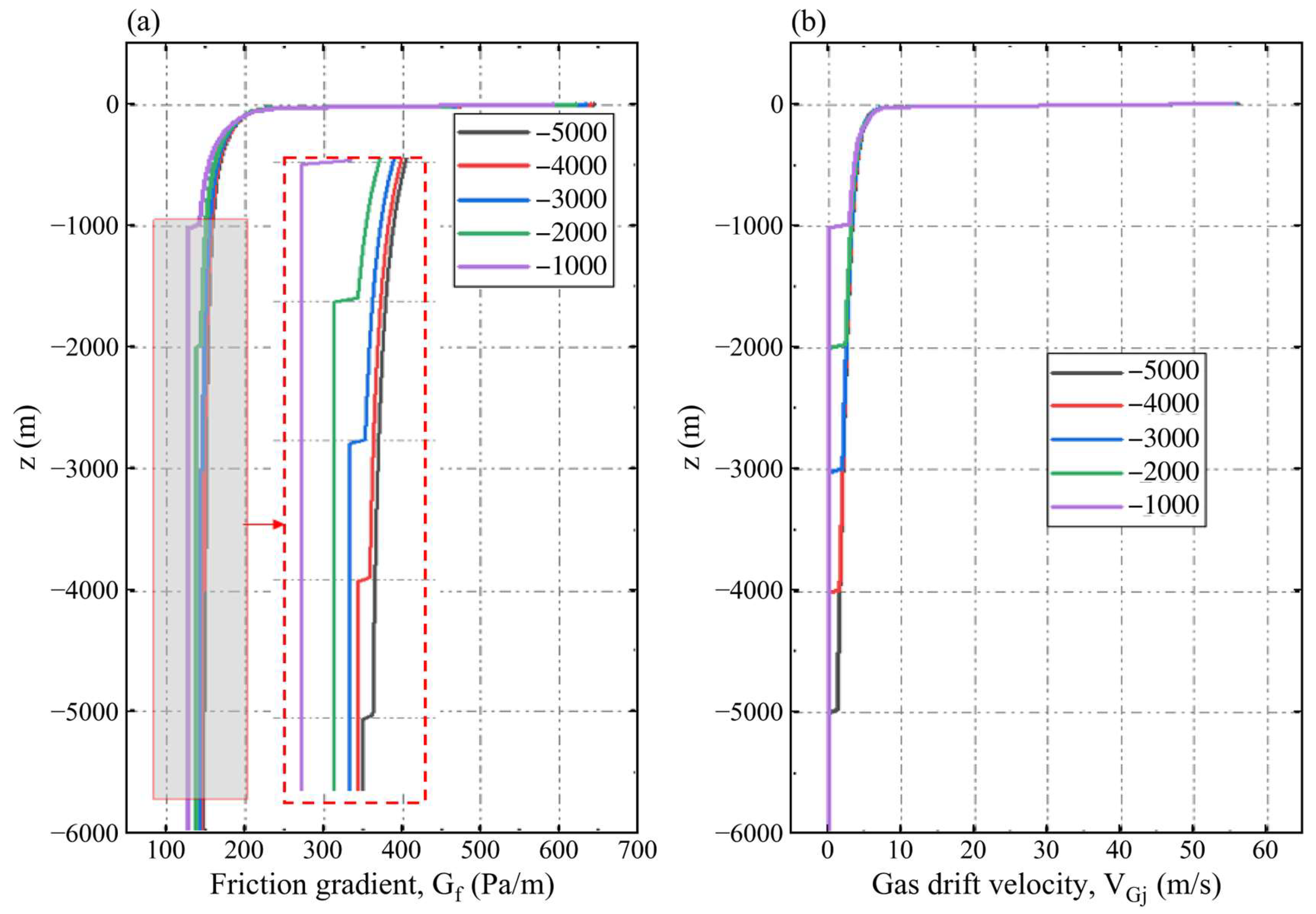
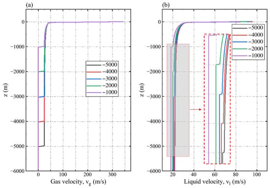
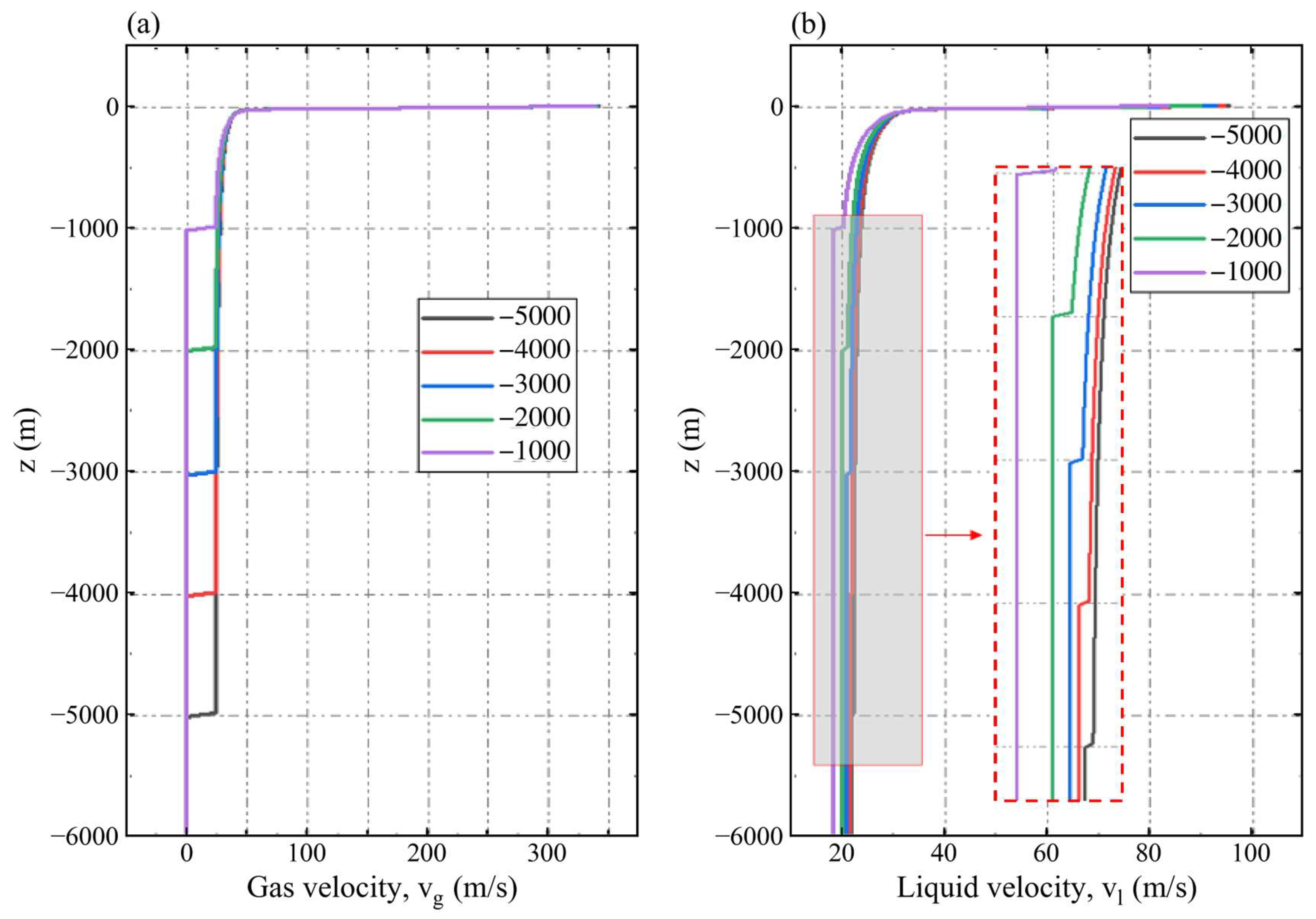
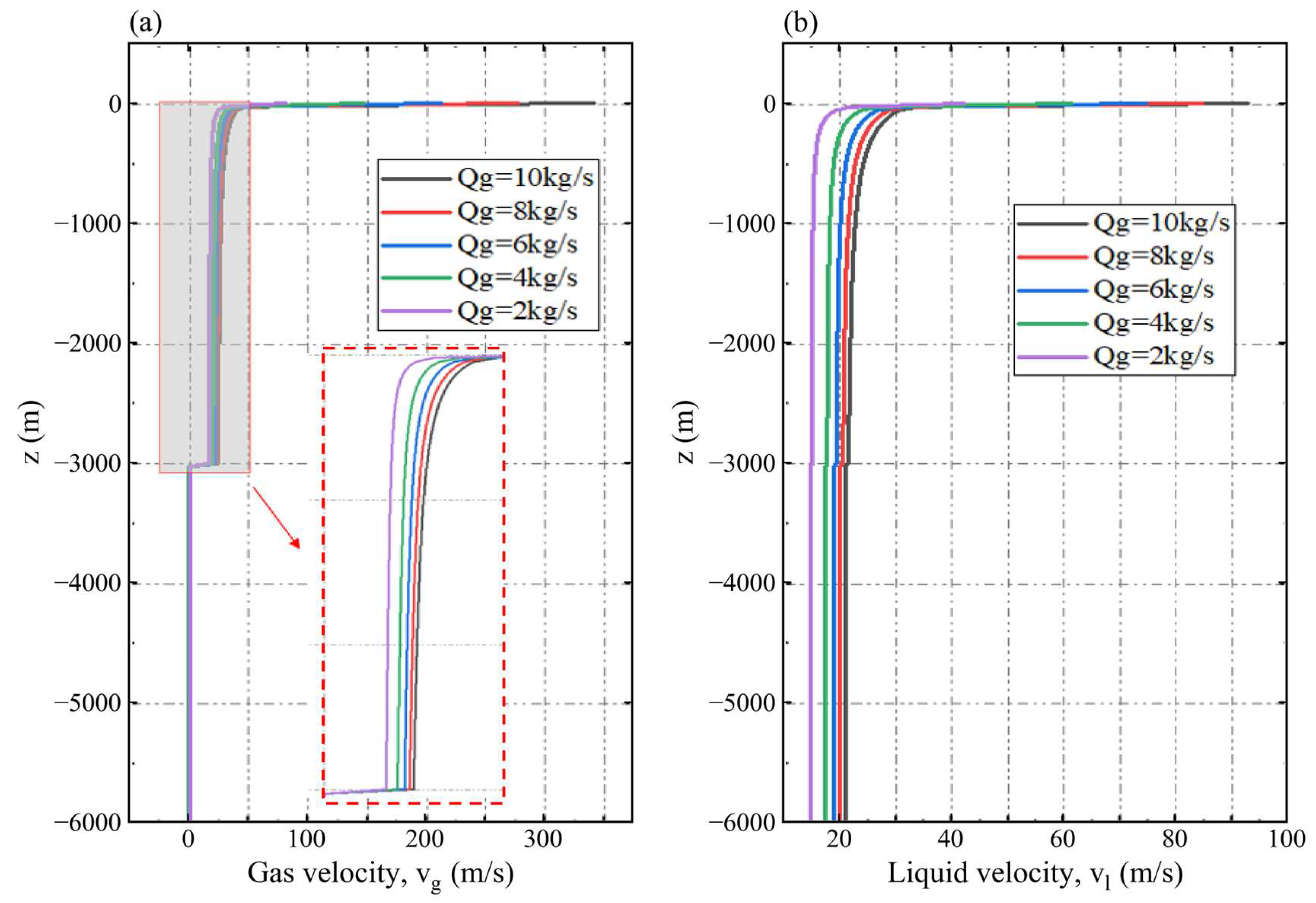
Figure 10 and Figure 11 resolve concentration-dependent resistance and phase velocity. For CX = 2%, 4%, 6%, 8%, and 10%, Δpf = ∫Gf dz over −6000 ≤ z ≤ 0 m is approximately 0.257, 0.486, 0.661, 0.800, and 0.899 MPa, respectively. Corresponding slurry flows are approximately 0.750, 0.714, 0.687, 0.669, and 0.651 m³/s (Table 10). From 2% to 10%, throughput falls by about 13.2% and frictional loss rises to about 3.5 times the value at 2% concentration.

Figure 10. Axial wall friction pressure gradient (a) and gas drift velocity (b) for the concentration series.

Figure 11. Axial gas velocity (a) and liquid velocity (b) for the concentration series.

Table 10. Approximate slurry discharge and frictional pressure loss for the concentration series; D = 0.20 m, L = 6000 m, hinj = 3000 m, and gas input 10 kg/s.

CX (%)	Qsl (m3/s)	Δpf (MPa)
2	0.750	0.257
4	0.714	0.486
6	0.687	0.661
8	0.669	0.800
10	0.651	0.899

Gf and its integral quantify the constitutive effect over the represented shear-rate range; the units of K depend on n. The hydraulic balance combines gas lift driving head, suspension density, friction, and axial acceleration. Lower-concentration cases have lower frictional losses and higher throughput under the shared settings.

Figure 9, Figure 10 and Figure 11 thus show similar large-scale gas-holdup patterns together with concentration-dependent hydraulic performance. The homogeneous power law formulation predicts averaged suspension transportation throughout the tested range and quantifies the associated resistance and discharge. These quantities provide the basis for comparing slurry transport conditions.

$$\Delta p_f={\int }_{-6000}^0{G}_f\left(z\right)\hspace{0.17em}\mathrm{d}z, G_f={\displaystyle \frac{4{\tau }_w}{D}} \left[\mathrm{P}\mathrm{a}/\mathrm{m}\right].$$

(52)

Qsl is suspension volume flow; Δpf is the frictional component integrated over the common plotted riser interval.

5.3. Injection Depth and Relative Lifting Performance

Relative lifting performance is ηi = Qsl,i/Qsl,a, the dimensionless ratio of outlet slurry throughput to the reference discharge within each series. The outlet flux is Qsl = A(1 − αg,out)vl,out = Ajl,out, where vl,out is intrinsic liquid velocity and jl,out is its superficial value. This index measures normalized hydraulic throughput.

The depth series uses D = 0.20 m, L = 6000 m, CX = 0.10, and gas input 10 kg/s. For hinj = 1000, 2000, 3000, 4000, and 5000 m, the recalculated relative lifting performance is approximately 0.827, 0.906, 0.947, 0.980, and 1.000, respectively. Table 11 uses the reported discharge of Case 3-a at 5000 m, Qsl,a = 0.694 m³/s, as the common reference for this series.

$${\eta }_i={\displaystyle \frac{Q_{\mathrm{s}\mathrm{l},i}}{Q_{\mathrm{s}\mathrm{l},a}}}.$$

(53)

Table 11. Injection depth series and within-series relative lifting performance.

Case	hinj (m)	Qsl (m3/s)	Δpf (MPa)	η (–)
3-a	5000	0.694	0.95	1.000
3-b	4000	0.680	0.92	0.980
3-c	3000	0.657	0.90	0.947
3-d	2000	0.629	0.87	0.906
3-e	1000	0.574	0.80	0.827

Common settings: D = 0.20 m, L = 6000 m, CX = 0.10, and gas input 10 kg/s. Qsl and Δpf are approximate profile-based hydraulic values. Each η is calculated directly from the Qsl values listed in this table using Qsl,a = 0.694 m³/s. The derived indices are reported to three decimal places and percentage comparisons to one decimal place, consistent with the approximate discharge values.

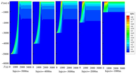
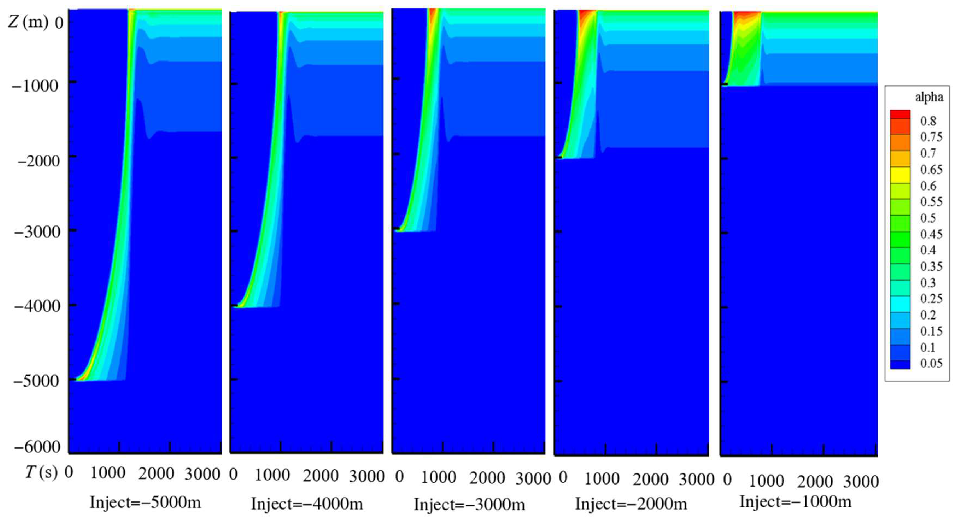
Figure 12 shows that injection depth changes the extent and evolution of the gas-containing lifting section. At 1000–2000 m, gas expansion, mixture density changes, and liquid acceleration occur over a shorter distance, producing more localized start-up gas-holdup variation. Deeper injection distributes this hydraulic evolution over a longer lifting section.

Figure 12. Gas-holdup evolution for injection depths of 5000, 4000, 3000, 2000, and 1000 m, from left to right.

The contours compare the axial extent and timing of gas-holdup evolution. The late-time resistance and phase velocities in Figure 13 and Figure 14 then provide the complementary information used to quantify slurry throughput.

Figure 13. Axial wall friction pressure gradient (a) and gas drift velocity (b) for the injection depth series.

Figure 14. Axial gas velocity (a) and liquid velocity (b) for the injection depth series.

For hinj = 1000, 2000, 3000, 4000, and 5000 m, approximate slurry flows are 0.574, 0.629, 0.657, 0.680, and 0.694 m³/s, with frictional losses over −6000 ≤ z ≤ 0 m of approximately 0.80, 0.87, 0.90, 0.92, and 0.95 MPa. Deeper injection increases both throughput and the opposing frictional loss. The net trend reflects the combined effects of gas-containing lifting length, density distribution, and hydraulic resistance.

For each additional 1000 m, the relative throughput increments, calculated as 100(Qsl,new/Qsl,old − 1), are approximately 9.6%, 4.5%, 3.5%, and 2.1%. Throughput therefore increases with diminishing incremental gains. Gas holdup and intrinsic liquid velocity jointly determine the outlet flux, while the discharge and frictional loss comparisons quantify the net hydraulic response.

The 3000 m case provides approximately 94.7% of the 5000 m reference throughput. Further deepening to 5000 m raises throughput by approximately 5.6% relative to the 3000 m value. The largest throughput occurs at 5000 m; diminishing increments make 3000 m a useful intermediate condition for the gas input comparison. This hydraulic trade-off can support installation-specific assessment alongside compressor performance and operating objectives.

5.4. Gas Mass Flow and Relative Lifting Performance

The gas input series fixes D = 0.20 m, L = 6000 m, CX = 0.10, and hinj = 3000 m and varies final gas mass flow ṁg from 2 to 10 kg/s. Its reference is Case 4-a at 10 kg/s, with the reported discharge Qsl,a = 0.659 m³/s. All indices in Table 12 are recalculated from the discharges listed in that table. The depth and gas input series are normalized separately, each against its own case a reference.

Table 12. Gas mass flow series and within-series relative lifting performance.

Case	ṁg (kg/s)	Qsl (m3/s)	Δpf (MPa)	η (–)
4-a	10	0.659	0.90	1.000
4-b	8	0.627	0.86	0.951
4-c	6	0.595	0.82	0.903
4-d	4	0.546	0.77	0.829
4-e	2	0.465	0.67	0.706

Common settings: D = 0.20 m, L = 6000 m, CX = 0.10, and hinj = 3000 m. Qsl and Δpf are approximate profile-based hydraulic values. Each η is calculated directly from the Qsl values listed in this table using Qsl,a = 0.659 m³/s. The derived indices are reported to three decimal places and percentage comparisons to one decimal place, consistent with the approximate discharge values.

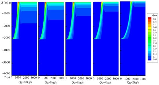
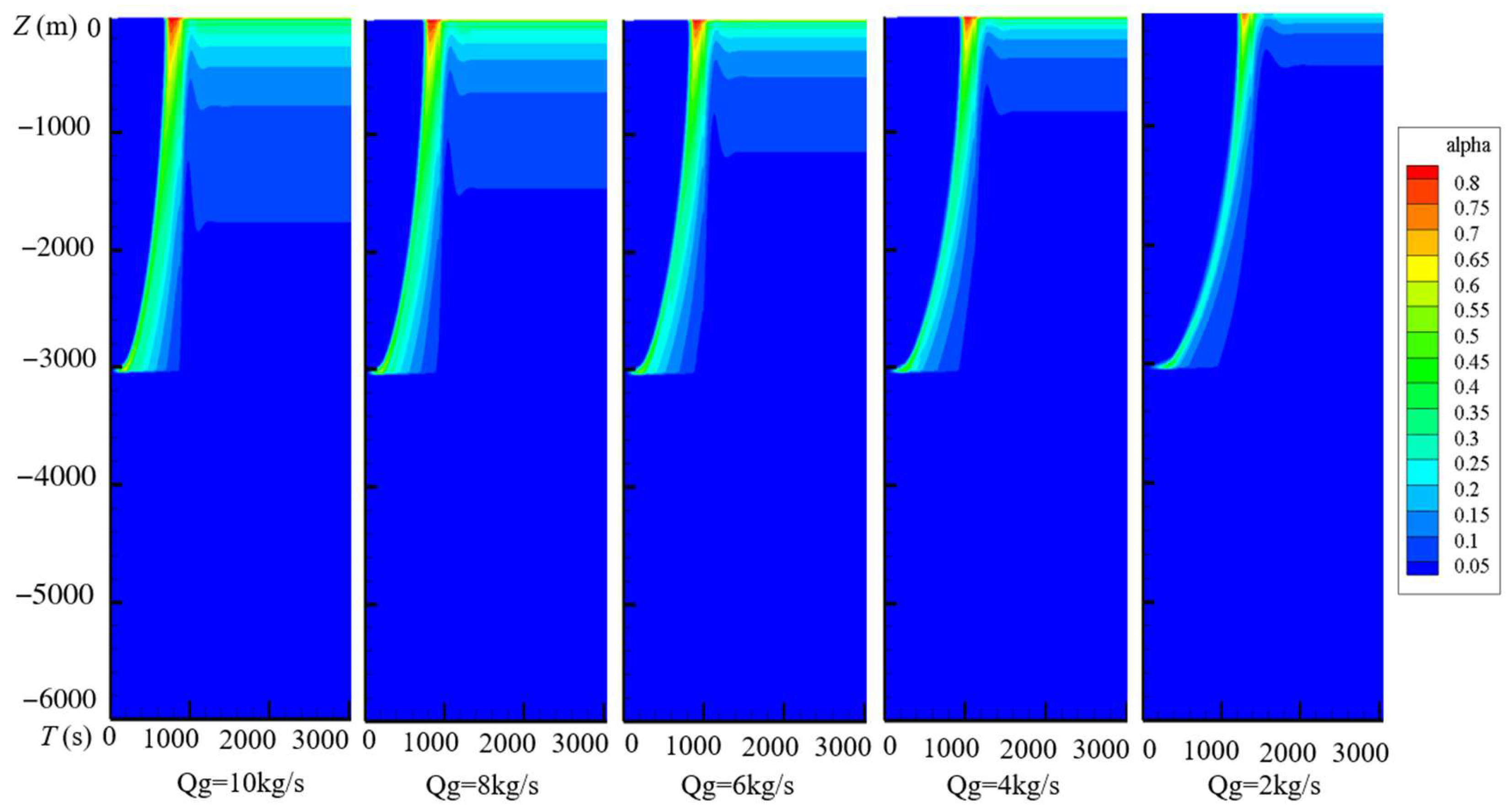
Figure 15 shows how increasing gas input expands the gas-containing region and changes the local gas fraction. The 8 and 10 kg/s cases have similar overall late-time patterns, whereas lower inputs produce a more spatially restricted distribution. These histories give the spatial and temporal context for the hydraulic comparison.

Figure 15. Gas-holdup evolution for gas mass inputs of 10, 8, 6, 4, and 2 kg/s, from left to right.

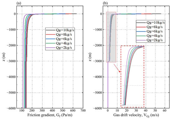
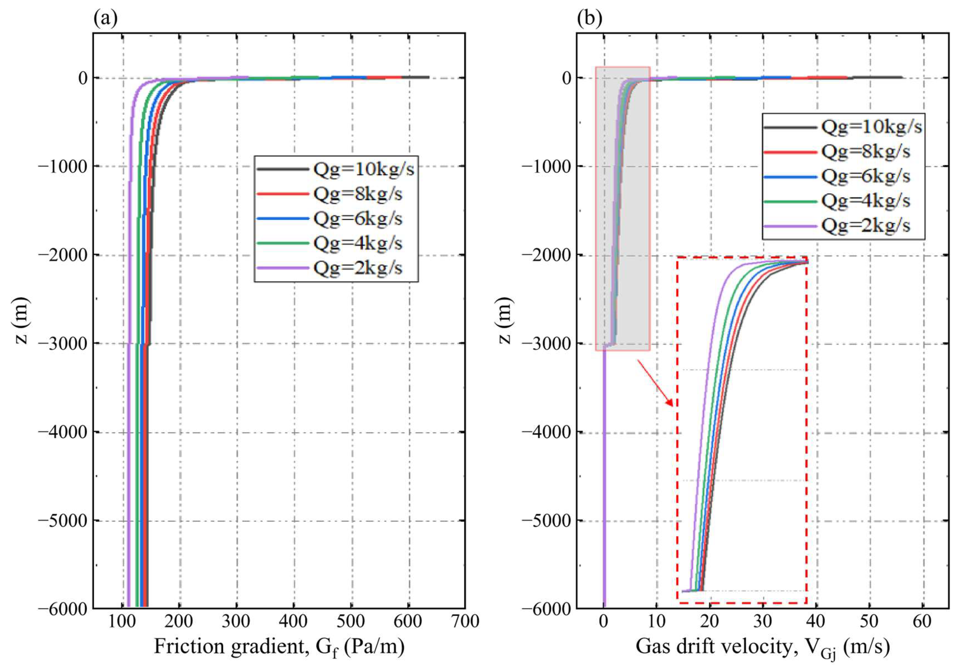
Gas supply changes gas content, mixture density, and the driving force for lifting. Absolute pressure also determines gas density, coupling these changes to the axial pressure distribution. Figure 16 and Figure 17 show the accompanying resistance and phase velocities under the shared geometry and material conditions.

Figure 16. Axial wall friction pressure gradient (a) and gas drift velocity (b) for the gas input series.

Figure 17. Axial gas velocity (a) and liquid velocity (b) for the gas input series.

For gas inputs of 2, 4, 6, 8, and 10 kg/s, approximate slurry flows are 0.465, 0.546, 0.595, 0.627, and 0.659 m³/s, and frictional losses integrated over −6000 ≤ z ≤ 0 m are 0.67, 0.77, 0.82, 0.86, and 0.90 MPa. Increasing gas input strengthens the driving force for lifting and increases both throughput and frictional loss. Conversely, lower gas input produces a weaker driving force, lower discharge, and lower resistance.

Table 12 gives recalculated η values of approximately 0.706, 0.829, 0.903, 0.951, and 1.000 for gas inputs of 2, 4, 6, 8, and 10 kg/s. Each additional 2 kg/s raises throughput by approximately 17.4%, 9.0%, 5.4%, and 5.1%, respectively. Friction opposes the flow, while the net throughput gain remains positive throughout the investigated range with diminishing increments.

The 8 kg/s case achieves approximately 95.1% of the reference throughput with 80% of its gas input. Increasing the gas supply from 8 to 10 kg/s requires 25% more gas and increases throughput by approximately 5.1%; the largest throughput occurs at 10 kg/s. These values quantify an intermediate hydraulic trade-off. Installation-specific selection also depends on compressor performance, terminal discharge, and operating objectives.

6. Conclusions

A one-dimensional drift flux framework has been used to examine material replacement during start-up and hydraulic transportation of homogeneous power law rare earth slurry in a long riser. The formulation couples gas compressibility, relative phase motion, slurry constitutive response, and wall friction. The assessments separately cover the outlet scalar, single-phase power law flow, and Newtonian air–water discharge. The slurry calculations provide predictions under the stated closures and numerical resolution. The principal findings are as follows.

The formulation represents initial water replacement by incoming suspension through liquid volume accounting and material property assignment. Comparison with the liquid–gas reference illustrates sensitivity of the predicted gas-holdup field to this treatment. The analytical comparison verifies the selected single-phase power law response, while the air–water experiments assess Newtonian liquid discharge, with pooled MARD and MRD of 5.79% and +4.27%. These component assessments are distinguished from direct experimental validation of coupled non-Newtonian slurry lifting.

The independently prescribed outlet diagnostic gives Mh = 4.1216 at the outlet face, 1.0590 at the center 5 m upstream, and 0.4576 at 15 m. Every gas-containing interior center retains an upstream-propagating drift flux characteristic. The homogeneous indicator and coupled characteristics locate a pronounced terminal response under the prescribed pressure outlet; both samples above unity remain part of the interpretation.

Similar overall gas-holdup patterns coexist with concentration-dependent resistance and throughput. Increasing CX from 2% to 10% reduces approximate slurry discharge from 0.750 to 0.651 m³/s, by about 13.2%, and raises frictional loss from 0.257 to 0.899 MPa under the common geometry and gas input. The concentration effect is therefore quantified through the suspension’s averaged hydraulic response rather than inferred from contour appearance alone.

Greater injection depth and gas mass flow increase throughput with diminishing incremental gains. The 3000 m case provides approximately 94.7% of the 5000 m reference throughput; the 8 kg/s case provides approximately 95.1% of the 10 kg/s reference at 3000 m. The increase in frictional losses opposes the increase in transportation rates. These within-series comparisons quantify trade-offs among gas supply, lifting length, resistance, and slurry throughput for installation-specific assessment.

References

- Falconnet, P. The economics of rare earths. J. Less Common Met. 1985, 111, 9–15. [Google Scholar] [CrossRef] [Scilit]
- Humphries, M. Rare Earth Elements: The Global Supply Chain; CRS Report for Congress, R41347; Congressional Research Service, Library of Congress: Washington, DC, USA, 2010. [Google Scholar]
- Alonso, E.; Sherman, A.M.; Wallington, T.J.; Everson, M.P.; Field, F.R.; Roth, R.; Kirchain, R.E. Evaluating Rare Earth Element Availability: A Case with Revolutionary Demand from Clean Technologies. Environ. Sci. Technol. 2012, 46, 3406–3414. [Google Scholar] [CrossRef] [Scilit]
- Bao, Z.; Zhao, Z. Geochemistry of mineralization with exchangeable REY in the weathering crusts of granitic rocks in South China. Ore Geol. Rev. 2008, 33, 519–535. [Google Scholar] [CrossRef] [Scilit]
- Zhao, X.; Li, N.-B.; Huizenga, J.M.; Yan, S.; Yang, Y.-Y.; Niu, H.-C. Rare earth element enrichment in the ion-adsorption deposits associated granites at Mesozoic extensional tectonic setting in South China. Ore Geol. Rev. 2021, 137, 104317. [Google Scholar] [CrossRef] [Scilit]
- Weng, Z.; Jowitt, S.M.; Mudd, G.M.; Haque, N. A detailed assessment of global rare earth element resources: Opportunities and challenges. Econ. Geol. 2015, 110, 1925–1952. [Google Scholar] [CrossRef] [Scilit]
- Weng, Z.; Jowitt, S.; Mudd, G.; Haque, N. Assessing rare earth element mineral deposit types and links to environmental impacts. Appl. Earth Sci. 2013, 122, 83–96. [Google Scholar] [CrossRef] [Scilit]
- Kon, Y.; Hoshino, M.; Sanematsu, K.; Morita, S.; Tsunematsu, M.; Okamoto, N.; Yano, N.; Tanaka, M.; Takagi, T. Geochemical characteristics of apatite in heavy REE rich deep-sea mud from Minamitorishima area, southeastern Japan. Resour. Geol. 2014, 64, 47–57. [Google Scholar] [CrossRef] [Scilit]
- Kato, Y.; Fujinaga, K.; Nakamura, K.; Takaya, Y.; Kitamura, K.; Ohta, J.; Toda, R.; Nakashima, T.; Iwamori, H. Deep-sea mud in the Pacific Ocean as a potential resource for rare-earth elements. Nat. Geosci. 2011, 4, 535–539. [Google Scholar] [CrossRef] [Scilit]
- Iijima, K.; Yasukawa, K.; Fujinaga, K.; Nakamura, K.; Machida, S.; Takaya, Y.; Ohta, J.; Haraguchi, S.; Nishio, Y.; Usui, Y.; et al. Discovery of extremely REY-rich mud in the western North Pacific Ocean. Geochem. J. 2016, 50, 557–573. [Google Scholar] [CrossRef] [Scilit]
- Kashiwabara, T.; Toda, R.; Fujinaga, K.; Honma, T.; Takahashi, Y.; Kato, Y. Determination of host phase of lanthanum in deep-sea REY-rich mud by XAFS and m-XRF using high-energy synchrotron radiation. Chem. Lett. 2014, 43, 199–200. [Google Scholar] [CrossRef] [Scilit]
- Machida, S.; Fujinaga, K.; Ishii, T.; Nakamura, K.; Hirano, N.; Kato, Y. Geology and geochemistry of ferromanganese nodules in the Japanese Exclusive Economic Zone around Minamitorishima Island. Geochem. J. 2016, 50, 539–555. [Google Scholar] [CrossRef] [Scilit]
- Sha, F.; Xi, M.; Chen, X.; Liu, X.; Niu, H.; Zuo, Y. A recent review on multi-physics coupling between deep-sea mining equipment and marine sediment. Ocean Eng. 2023, 276, 114229. [Google Scholar] [CrossRef] [Scilit]
- Wang, L.; Cheng, L.; Yin, S.; Yan, Z.; Zhang, X. Multiphase slurry flow regimes and its pipeline transportation of underground backfill in metal mine: Mini review. Constr. Build. Mater. 2023, 402, 133014. [Google Scholar] [CrossRef] [Scilit]
- Shimizu, Y.; Hatakeyama, N.; Hanamura, E.; Watanabe, K.; Yokoyama, Y.; Masuyama, T. Flow Characteristics of Slurry with Rare-Earth Rich Mud under Deep Seabed around Minamitorishima. J. MMIJ 2019, 135, 52–62. [Google Scholar] [CrossRef] [Scilit]
- Shimizu, Y.; Hatakeyama, N.; Masuyama, T. Numerical Analysis on Air-Lift Pumping System for Mining Rare-Earth Rich Mud. J. MMIJ 2018, 134, 142–150. [Google Scholar] [CrossRef] [Scilit]
- Yamazaki, T.; Nakatani, N.; Arai, R.; Sekimoto, T.; Katayama, H. Combined Mining and Pulp-Lifting of Ferromanganese Nodules and Rare-Earth Element-Rich Mud around Minamitorishima Island in the Western North Pacific: A Prefeasibility Study. Minerals 2021, 11, 310. [Google Scholar] [CrossRef] [Scilit]
- Fan, W.; Chen, J.; Pan, Y.; Huang, H.; Chen, C.-T.A.; Chen, Y. Experimental study on the performance of an air-lift pump for artificial upwelling. Ocean Eng. 2013, 59, 47–57. [Google Scholar] [CrossRef] [Scilit]
- Kim, S.H.; Sohn, C.H.; Hwang, J.Y. Effects of tube diameter and submergence ratio on bubble pattern and performance of air-lift pump. Int. J. Multiph. Flow 2014, 58, 195–204. [Google Scholar] [CrossRef] [Scilit]
- Khalil, M.F.; Elshorbagy, K.; Kassab, S.; Fahmy, R. Effect of air injection method on the performance of an air lift pump. Int. J. Heat Fluid Flow 1999, 20, 598–604. [Google Scholar] [CrossRef] [Scilit]
- Wang, Q.; Liu, Y.; Luo, J.; Wang, S.; He, W.; Zhang, S.; Chen, G. Experimental research on the performance of a gas lift bubble pump based on a diffusion generation process. Appl. Therm. Eng. 2021, 185, 116060. [Google Scholar] [CrossRef] [Scilit]
- Wu, J.; Cao, W.; Cong, T. Numerical investigation on the performance of gas-lift pump with large density ratio of liquid to gas. Int. J. Multiph. Flow 2022, 148, 103936. [Google Scholar] [CrossRef] [Scilit]
- Pougatch, K.; Salcudean, M. Numerical modelling of deep sea air-lift. Ocean Eng. 2008, 35, 1173–1182. [Google Scholar] [CrossRef] [Scilit]
- Du, W.; Fu, T.; Duan, Y.; Zhu, C.; Ma, Y.; Li, H.Z. Breakup dynamics for droplet formation in shear-thinning fluids in a flow-focusing device. Chem. Eng. Sci. 2018, 176, 66–76. [Google Scholar] [CrossRef] [Scilit]
- Salehi, M.S.; Esfidani, M.T.; Afshin, H.; Firoozabadi, B. Experimental investigation and comparison of Newtonian and non-Newtonian shear-thinning drop formation. Exp. Therm. Fluid Sci. 2018, 94, 148–158. [Google Scholar] [CrossRef] [Scilit]
- Kant, K.; Banerjee, R. Effect of density ratios on droplet breakup for newtonian and power-law fluids. Int. J. Multiph. Flow 2023, 167, 104561. [Google Scholar] [CrossRef] [Scilit]
- Xu, X.; Zhang, J.; Liu, F.; Wang, X.; Wei, W.; Liu, Z. Rising behavior of single bubble in infinite stagnant non-Newtonian liquids. Int. J. Multiph. Flow 2017, 95, 84–90. [Google Scholar] [CrossRef] [Scilit]
- Fu, T.; Ma, Y.; Li, H.Z. Bubble coalescence in non-Newtonian fluids in a microfluidic expansion device. Chem. Eng. Process. Process Intensif. 2015, 97, 38–44. [Google Scholar] [CrossRef] [Scilit]
- Liu, Y. Development of a wide range numerical model for gas-lift pump system in deep sea mining based on void fraction correlated drift flux model. Ships Offshore Struct. 2025, 1–19. [Google Scholar] [CrossRef] [Scilit]
- Lemmon, E.W.; Jacobsen, R.T.; Penoncello, S.G.; Friend, D.G. Thermodynamic Properties of Air and Mixtures of Nitrogen, Argon, and Oxygen From 60 to 2000 K at Pressures to 2000 MPa. J. Phys. Chem. Ref. Data 2000, 29, 331–385. [Google Scholar] [CrossRef] [Scilit]
- Kajishima, T.; Saito, T. Numerical Simulation of Unsteady Flow in Air-Lift Pump. JSME Int. J. Ser. B 1996, 39, 525–532. [Google Scholar] [CrossRef] [Scilit]
- Ishii, M. One-Dimensional Drift-Flux Model and Constitutive Equations for Relative Motion Between Phases in Various Two-Phase Flow Regimes; ANL-77-47; Argonne National Laboratory: Argonne, IL, USA, 1977; Available online: https://digital.library.unt.edu/ark:/67531/metadc283216/ (accessed on 22 October 2026).
- Hatakeyama, N.; Shimizu, Y.; Masuyama, T. Constitutive Equations for a Simulator of Airlift Pump in a Large Diameter Pipe using Drift-Flux Model. J. MMIJ 2018, 134, 31–40. [Google Scholar] [CrossRef] [Scilit][Green Version]
- Kataoka, I.; Ishii, M. Drift Flux Model for Large Diameter Pipe and New Correlation for Pool Void Fraction. Int. J. Heat Mass Transf. 1987, 30, 1927–1939. [Google Scholar] [CrossRef] [Scilit]
- Fang, X.; Xu, Y.; Zhou, Z. New correlations of single-phase friction factor for turbulent pipe flow and evaluation of existing single-phase friction factor correlations. Nucl. Eng. Des. 2011, 241, 897–902. [Google Scholar] [CrossRef] [Scilit]
- Metzner, A.B.; Reed, J.C. Flow of non-Newtonian fluids—Correlation of the laminar, transition, and turbulent-flow regions. AIChE J. 1955, 1, 434–440. [Google Scholar] [CrossRef] [Scilit]
- Sanderse, B.; Eskerud Smith, I.; Hendrix, M.H.W. Analysis of time integration methods for the compressible two-fluid model for pipe flow simulations. Int. J. Multiph. Flow 2017, 95, 155–174. [Google Scholar] [CrossRef] [Scilit]
- Weber, M.; Dedegil, Y. Transport of solids according to the air-lift principle. In Proceedings of the 4th International Conference on the Hydraulic Transport of Solids in Pipes (Hydrotransport 4), Banff, AB, Canada, 18–21 May 1976; pp. 1–23. [Google Scholar]
- Usami, T.; Saito, T.; Kitahara, R. Lifting Characteristics of Solid by Air Lift Pump (2nd Report): Sea test with simulated manganese nodules. J. Min. Metall. Inst. Jpn. 1982, 98, 29–34. [Google Scholar] [CrossRef] [Scilit][Green Version]
- Saito, T.; Usami, T.; Yamazaki, T.; Tomishima, Y.; Kiyono, F.; Shimizu, Y. Analysis of Lifting Characteristics of Manganese Nodules by Air Lift Pump by Means of Dimensionless Parameter. Shigen-to-Sozai 1991, 107, 265–270. [Google Scholar] [CrossRef] [Scilit]
- Saito, T.; Kajishima, T.; Tsuchiya, K. Pumping characteristics of a large-scale gas-lift system. Exp. Therm. Fluid Sci. 2004, 28, 479–488. [Google Scholar] [CrossRef] [Scilit]
- Brennen, C.E. Chapter 6: Homogeneous Bubbly Flows. In Cavitation and Bubble Dynamics; Oxford University Press: New York, NY, USA, 1995; Available online: https://media.library.caltech.edu/CaltechBOOK:1995.001/chap6.htm (accessed on 22 October 2026).
Disclaimer/Publisher’s Note: The statements, opinions and data contained in all publications are solely those of the individual author(s) and contributor(s) and not of MDPI and/or the editor(s). MDPI and/or the editor(s) disclaim responsibility for any injury to people or property resulting from any ideas, methods, instructions or products referred to in the content. |
© 2026 by the author. Licensee MDPI, Basel, Switzerland. This article is an open access article distributed under the terms and conditions of the Creative Commons Attribution (CC BY) license.