


Abstract
Capturing carbon dioxide at a climate-relevant scale is an energy supply problem as much as a separation problem. We developed a linked scenario model that follows capture mix, heat supply, and carbon fate through one balance of heat, electricity, generation, storage, land, and retained carbon. An illustrative 10 Gt CO2/year portfolio with 55% flue-gas capture, 25% already separated CO2, and 20% direct air capture (DAC) needs 30.25 EJ/year of process heat and 10.06 EJ/year of direct electricity. On an annual energy basis, dedicated wind and solar supply requires 5.37 TW of nameplate capacity with electric boilers, and 2.64 TW with heat pumps at a coefficient of performance of 3. Losing the already separated streams and drawing heat from a heat-pump source at 20 °C raises the requirement to 4.12 TW. Complete electrochemical DAC must use less than 3.47 GJ/t of precompression electricity to beat thermal DAC with heat pumps, and diverting 1 Gt/year of DAC CO2 to methanol more than doubles portfolio electricity while halving the atmospheric CO2 reaching geological storage. The results are scenario-dependent and identify heat integration, source availability, and carbon fate as screening criteria for process development and deployment planning.
1. Introduction
Carbon capture, utilization, and storage (CCUS) connects separation processes with energy supply, CO2 transport, and carbon management. Its energy demand becomes consequential at the gigatonne scale, but a single global energy-intensity estimate hides differences in source concentration, regeneration temperature, electricity supply, and carbon fate. A tonne of fossil CO2 captured before emission is a different climate service from a tonne removed from ambient air and durably stored. These distinctions have to be carried through any assessment of the infrastructure that large-scale deployment implies.
The scale is set by sectors that cannot be electrified outright. The Intergovernmental Panel on Climate Change (IPCC) attributes about a quarter of direct greenhouse gas emissions in 2019 to industry, with iron, steel, cement, and chemicals being the largest contributors, and identifies carbon capture as part of the mitigation portfolio for these process emissions, alongside residual emissions from aviation and shipping [1]. The IPCC assesses multiple pathways with differing roles for capture and removal and does not prescribe a single global capture requirement [1]. The International Energy Agency’s (IEA) 2021 Net Zero by 2050 scenario reported approximately 1.6 Gt CO2/year captured in 2030 and 7.6 Gt/year in 2050 across multiple activities, including atmospheric and biogenic pathways; the 2023 roadmap update lowered these volumes but kept capture and removal in the pathway [2,3]. Operating capture capacity in 2023 was around 45 Mt/year, two orders of magnitude below the 2050 scenario level [3]. We therefore use 10 Gt/year as a round-number gross-throughput scale test, near the upper end of the scenario range, with linear rescaling to other throughputs and explicit variation in the direct air capture (DAC) fraction.
The individual elements of this analysis have substantial precedents. The carbon capture and storage (CCS) literature has established process-energy penalties, integration opportunities, and cost boundaries [4]. McQueen et al. connected DAC solvent and sorbent properties with mass transfer, heat transfer, process designs, and scale-ups [5]. Sabatino et al. compared and optimized aqueous and solid-sorbent DAC processes using energy, exergy, productivity, and cost metrics [6]. These studies show why regeneration duty alone does not determine technology performance: cyclic productivity and equipment requirements matter as well.
Energy supply studies extend the process boundaries. Fasihi et al. coupled DAC heat and electricity requirements with renewable supply, heat pumps, and hourly operations [7]. The IEA’s DAC assessment identified energy supply, location, and process configurations as coupled deployment choices [8]. Young et al. combined engineering economic models and technological learning to evaluate four DAC and storage technologies; their analysis distinguishes plant utilization and financing from energy prices [9]. Hofmann et al. optimized interacting hydrogen and CO2 networks within a European energy system model, demonstrating that infrastructure and capture choices depend on the surrounding energy system [10]. These precedents motivate explicit supply assumptions and warn against reading annual energy balances as optimized electricity systems.
Process-specific heat pump studies provide further insight. Jensen et al. simulated heat recovery within an amine biogas-upgrading process using separate temperature levels, while Cremona et al. integrated heat pumps with capture, compression, and cement-plant heat sources [11,12]. Both studies evaluated heat-source and process configurations explicitly. Their results establish a basis for considering heat pump integration, while leaving the applicable coefficient of performance and recoverable duty dependent on plant design.
Life-cycle assessments (LCAs) likewise extend beyond operational energy. Deutz and Bardow assessed industrial temperature-vacuum swing adsorption, while Madhu et al. compared thermal DAC routes and their resource implications [13,14]. Bouaboula et al. examined electrochemical pH-swing DAC across its life cycle and subsequently compared high-temperature aqueous, temperature-vacuum swing, moisture-swing, and pH-swing approaches within a harmonized assessment [15,16]. Their work supports comparing technologies under consistent functions and assumptions rather than selecting one DAC route as universally preferable.
This study traces changes in capture mix, heat supply, and utilization through to generation capacity, storage, land, capital, and retained carbon in a single reproducible accounting. Established thermodynamic and process benchmarks provide the inputs; the contribution is linking them and the results that follow. The model is not a new capture process and not an energy-system optimization. Source substitution changes exposure to heat-pump performance; electrochemical capture must satisfy a complete-process electricity crossover; and utilization changes both power demand and the amount of atmospheric carbon retained. Three questions guide the analysis: How do heat source conditions and capture mix jointly change electricity demands? When can electrochemical DAC outperform thermal DAC at matched product conditions? How does utilization alter energy and infrastructure requirements for the climate service delivered?
Three linked results illustrate what the accounting adds to this study. First, the loss of already separated CO2 streams and a colder heat-pump source together raise the reference renewable capacity by 0.25 TW more than the sum of their separate effects, because the replacement flue-gas heat is supplied at the lower COP (Section 3.2.4). Second, the electricity that an electrochemical DAC process must beat is not a property of the electrochemical process alone; it moves from 1.64 to 7.25 GJe/t with the heat supply of the thermal alternative (Section 3.3). Third, diverting one-tenth of gross capture to methanol raises portfolio electricity by 135% while halving the atmospheric CO2 that reaches geological storage (Section 3.5). None of these results can be read from the capture duty, the heat supply, or the carbon fate considered one at a time.
The model connects process development to deployment decisions. Section 3.6 expresses the calculated generation and storage capacities as capital sensitivities at published unit costs; Section 3.7 reports how the inputs propagate to each output; and Section 4 discusses the conditional implications for deployment. As in our previous publication [17], the aim is to give technology developers and policymakers quantitative insight into what climate-relevant CCUS requires, so that process intensification, system integration, and operational flexibility can be judged by their effect on total infrastructure demand and retained carbon.
2. Materials and Methods
2.1. Functional Units, System Boundaries, and Scenario Weights
The primary functional unit is one tonne of gross CO2 captured or conditioned and delivered to durable storage. Annual energy totals use 109 tonnes per gigatonne and a 365-day year. Figure 1 distinguishes process heat, direct electricity, compression, and downstream transport and injection. The reference storage case sends all captured CO2 to geological storage. Utilization is a separate branch: it adds hydrogen and conversion requirements, and carbon re-release must be tracked. The source stream and carbon origin are recorded separately; feed concentration alone cannot determine whether storage constitutes removal.
Figure 1.
System boundary for carbon capture, utilization, and storage (CCUS). The quantified reference case has utilization fraction u = 0 and includes capture or conditioning, compression, and an explicit downstream energy allowance. The dashed utilization branch requires its own product-system analysis. Dedicated renewable generation is one supply option; it is not a physical requirement of CCUS. Heat-pump source heat and externally supplied process heat remain resource inputs.
Three source classes are used to avoid assigning a common process to heterogeneous industrial sectors. Flue gas represents an illustrative dilute combustion stream treated with an amine process. The CO2-rich (rich-CO2) class represents a stream already separated as part of a host process and requiring conditioning and compression. Its low incremental duty does not describe separation of arbitrary natural gas or synthesis gas. DAC represents atmospheric CO2 captured using a low-temperature thermal process, with alternatives assessed separately. No capture at aircraft or ship engines is mapped to an upstream industrial source.
The reference mass fractions are 0.55 for flue gas, 0.25 for rich CO2, and 0.20 for DAC. They are analyst-selected scenario weights, not estimated market shares, capacity forecasts, or an emission inventory. Each source class is given a material role so that the comparison exposes its different energy and carbon consequences: point sources carry most of the throughput, already separated streams are represented because their low incremental duty makes them distinct, and DAC is given one-fifth of the total so that atmospheric removal is material without dominating the balance. The weights are not attributed to an IEA scenario or to an inventory of available streams, and no claim is made that 2.5 Gt/year of already separated CO2 is available. Section 3.2.3 gives linear rescaling with throughput, and Section 3.7 and Supplementary File S2 show how these choices propagate to each output. This comparison mixture combines heat-intensive capture, conditioning of already separated streams, and atmospheric capture. To test its dependence on unverified rich-stream availability, a separate sensitivity analysis fixes DAC at 20% and replaces rich CO2 with flue gas until the rich fraction reaches zero. Let x be the DAC fraction and α = 0.6875 the flue-gas fraction within point sources. Then
wflue = α(1 − x), wrich = (1 − α)(1 − x), wDAC = x
The fractions sum to unity for every x. We vary x from zero to one while holding α fixed to isolate the capture-mix effect. This substitution changes the climate service delivered; it is not an optimization between interchangeable avoided-emission and removal options. A rich-CO2 stream with no allocated upstream separation duty is valid only where the same separation exists in the reference host process. Otherwise, that separation energy and its costs must be added. The same boundary applies to emissions: the energy used and the CO2 emitted by the upstream separation remain with the host process and are not counted again here, so the rich-CO2 class neither omits nor double-counts that separation where the host already performs it. Five flow quantities are distinguished throughout: gross CO2 captured or conditioned, CO2 utilized, CO2 to geological storage, atmospheric CO2 to geological storage, and net CO2 removed per tonne of stored atmospheric CO2. Energy quantities carry the subscript th for heat and e for electricity; unsubscripted totals are first-law sums and are identified as such.
2.2. Thermodynamic Reference Calculations
For a binary ideal mixture at common temperature and pressure, reversible separation work follows from the Gibbs energy of mixing [18,19]. On a one-mole feed basis, let y be the feed CO2 mole fraction, r the CO2 recovery, p the product purity, P = ry/p the product moles, B = 1 − P the residual-gas moles, and z = y(1 − r)/B the residual CO2 mole fraction. With φ(v) = v ln(v) + (1 − v) ln(1 − v), the work per mole of recovered CO2 is
At 298.15 K with R = 8.314462618 J mol−1 K−1, the flue-gas case y = 0.15, r = 0.90, and p = 0.99 gives P = 0.13636 mol, B = 0.86364 mol, and z = 0.017368 per mole of feed, and Equation (2) returns 6.232 kJ/mol of recovered CO2, or 0.1416 GJ/t at 44.0095 g/mol. For y = 420 × 10−6, r = 0.50, and p = 0.99, P = 2.1212 × 10⁻⁴ mol, B = 0.99979 mol, and z = 2.1004 × 10⁻⁴, the result is 19.895 kJ/mol or 0.4521 GJ/t. Increasing flue-gas recovery to 0.99 raises the minimum to 0.1530 GJ/t, and a 75% single-pass DAC recovery gives 0.4651 GJ/t. These are specification-dependent separation references, not measured process performance. The 420 ppm value is a fixed comparison basis, not a claim about the current global atmospheric mean. Product purity of 99% is a calculation specification; transport suitability also depends on water and individual impurities.
Heat and work cannot be divided indiscriminately to calculate thermodynamic efficiency. For heat supplied isothermally at temperature Th and an environment at T0, the associated reversible work potential is Q(1 − T0/Th). At T0 = 298.15 K, this factor is 0.242 for 120 °C heat and 0.201 for 100 °C heat. Full exergy efficiency must also account for material streams, finite temperature changes, and a consistent output boundary, as illustrated by Hoseinpoori et al. [20]. We therefore do not rank technologies by dividing summed thermal and electrical duties by minimum separation work. The reference portfolio illustrates why. Its mass-weighted first-law input of 4.03 GJ/t (Section 3.1) is 24 times the mass-weighted separation minimum of 0.168 GJ/t. Converting the 120 °C and 100 °C heat to work potential with the factors above gives 1.69 GJ/t of exergy input, 10 times the separation minimum and about 4 times the minimum once the ideal 0.265 GJ/t compression reference is added to the denominator. The “25-fold” gap often quoted for capture is therefore mostly a statement that low-grade heat is not work. The exergy-based ratios of 4 to 10 are boundary-qualified comparisons, not achievable efficiency gains: the numerator and denominator do not share a complete process boundary, and the ideal-gas compression reference is not a rigorous real-fluid bound.
The ideal-gas expression RT ln(P2/P1) gives 0.2648 GJ/t CO2 for isothermal compression from 1 to 110 bar at 298.15 K. It is an idealized reference, not a rigorous minimum for real CO2 through gas-to-dense-phase conditions. Real-fluid properties, cooling, dehydration, pressure losses, and the compression-pumping arrangement determine practical work. We use an explicit practical compression input rather than claiming a universal combined separation-compression floor.
2.3. Process-Energy Inputs and Technology Representation
Table 1 distinguishes the three source classes and their reference capture duties. Flue-gas regeneration uses 3.5 GJth/t at approximately 120 °C as a conventional-amine comparison, with no deployment year assigned. Rochelle provides the established amine benchmark context [21]. RTI reports reboiler duties of 3.75 GJ/t for 30 wt% monoethanolamine (MEA) and 2.40 GJ/t for a non-aqueous solvent; these are different solvent/process configurations [22]. The 2.5 GJth/t lower-demand case represents an advanced solvent or improved process, not generic MEA performance; 4.0 GJth/t is the higher-duty case. Process integration offers further opportunities, but does not justify universal additive percentage savings [23]. A separate one-at-a-time sensitivity uses 3.0 and 2.5 GJth/t while holding the other reference inputs constant.
Table 1.
Reference source allocation and capture duties. All duties are per tonne of gross CO2; heat and electricity remain separate energy carriers. Common compression and transport-injection duties are additional.
The common compression input is 0.36 GJe/t (100 kWh/t), with 0.32 to 0.40 GJe/t tested. It is applied to all three source classes, on the assumption that each stream reaches the compressor near atmospheric pressure; an already separated stream available at elevated pressure would need less compression work. Compression and transport depend on the source state, flow, route, and storage pressure; published engineering models provide methods for evaluating these dependencies [24]. Capture-stage electrical allowances are 0.35 GJe/t for flue gas, 0.10 for rich-CO2 conditioning, and 1.64 for thermal DAC. They are analyst-selected allowances for auxiliary equipment or stream conditioning, not measured duties quoted from a particular plant. They remain separate from compression; impurity removal or a different incoming pressure may change the rich-stream allowance. Transport and injection add 0.10 GJe/t in the reference storage case, with 0 to 0.30 tested. This is an allowance, not a routed network model. The zero case is an accounting lower endpoint and does not imply that all transport and injection are energy-free.
Low-temperature thermal DAC uses 5.5 GJth/t at approximately 100 °C and 1.64 GJe/t before compression. The heat range of 4 to 8 GJth/t and electrical range of 1 to 2.5 GJe/t are selected sensitivities informed by published DAC assessments [7,13]. A common 0.36 GJe/t compression term raises the reference DAC electricity to 2.0 GJe/t at the compression boundary. The capture allowance includes air movement, vacuum, circulation, and cooling, so these should not be added again. These selected inputs do not reproduce the Hinwil or Hellisheiði plant inventories and do not establish that the thermal route is the best or insensitive to climate.
High-temperature aqueous DAC, moisture-swing DAC, and electrochemical DAC remain explicit alternatives. Keith et al. reported a liquid-DAC design using either 8.81 GJ of natural gas or 5.25 GJ of natural gas plus 366 kWh of electricity per tonne of atmospheric CO2, with CO2 delivered at 15 MPa [25]. Those fuel inputs and product conditions cannot be substituted directly for low-temperature regeneration heat and 110 bar compression. Moisture-swing operation likewise requires attention to water management and product conditioning. The harmonized comparison of Bouaboula et al. demonstrates why climate, energy prices, and coproducts belong in technology selection [16].
Electrochemical routes also have different functions and boundaries. Seo and Hatton reported an estimated minimum electrical work of 65 kJe/mol CO2 for their neutral-red cycle at a 410 ppm feed, equivalent to 1.48 GJe/t [26]. This cycle estimate differs from both a thermodynamic minimum for arbitrary separation and measured complete-plant electricity. Voskian and Hatton’s earlier electroswing results used feeds of 0.6 to 10% CO2; those measurements should not be relabeled as atmospheric-air performance [27]. Electrochemical pH-swing systems that coproduce hydrogen constitute another configuration [28]. Their gross electrical requirement must serve both products and cannot be compared with a capture-only process without a matching hydrogen reference.
Table 2 places these technology classes on a common footing. Energy values are the reference inputs and published figures used in this study, each quoted at its own boundary, so they show the form of the energy demand and the maturity of each class rather than a single ranking. Conventional amine scrubbing is the only class operating at the million-tonne scale on dilute flue gas [4,21]. Low-temperature solid-sorbent DAC and high-temperature aqueous DAC operate at demonstration to early commercial scale [5,8,13,25]. Electrochemical capture, including electroswing adsorption, pH-swing, and bipolar-membrane processes, remains at the laboratory and bench scale, with reported cell-level requirements that exclude auxiliaries and product handling [26,27,28,29]. The table explains why the model treats heat and electricity as separate carriers and tests electrochemical routes through the crossover condition in Section 2.6 rather than through a single energy number.
Table 2.
Capture technology classes as represented in this study. Energy values are quoted at the boundary stated for each entry and are not directly comparable across rows; th and e denote heat and electricity. Maturity descriptors follow the cited sources. DAC denotes direct air capture.
2.4. Conversion from Process Duties to Electricity Demand
For source i, let qi denote delivered process heat and ei capture-stage electricity, both in GJ/t. Let ci be compression electricity and di downstream transport-injection electricity. Annual thermal and direct electrical requirements are:
When M is in Gt/year, these products are in EJ/year. Delivered electricity depends on the heat-supply route:
Here χi is the electrical input per unit of process heat. For an electric boiler, χi = 1/ηb with ηb = 0.98. For a heat pump supplying all process heat, χi = 1/COPi, where COP is the heating coefficient of performance. If fraction hi of the process heat is supplied externally at the required temperature, χi = (1 − hi)/COPi for the remaining heat. Fully external heat sets χi = 0 while retaining the external heat demand, its emissions, and its cost.
The reference COP of three assumes process heat at 120 °C for flue-gas capture and 100 °C for DAC, with effective source temperatures of 70 and 50 °C, respectively. Allowing a 5 K approach on each side gives condensing/evaporating temperatures of 125/65 °C and 105/45 °C. The corresponding Carnot heating COPs are 6.64 and 6.30; COP three represents 45.2% and 47.6% of those values. These are specified heat-integration conditions, informed by the temperature-lift dependence in the heat-pump literature [30]. Source heat is Qhp minus compressor electricity and is retained as a separate resource requirement. Section 2.8 introduces a temperature sensitivity to test colder sources.
Internal heat recovery is a candidate supply for this requirement. Stripper-overhead condensation, lean-solvent cooling, and absorber intercooling can feed a heat pump; Jensen et al. use distinct evaporator levels to recover heat from these streams [11]. At COP three, the reference requires 12.83 EJ/year of source heat for flue-gas capture and 7.33 EJ/year for DAC, at effective source temperatures of 70 and 50 °C, respectively. These are evaporator duties, not necessarily demands for heat imported from outside the capture plant. Closing the internal supply requires temperature-duty profiles after existing heat recovery, exchanger approaches, and operating schedules. Total heat rejection alone does not demonstrate that this quantity is available at those temperatures. For cyclic DAC, sensible-heat recovery during cooling and heat from product condensation, where present, are candidates for process integration; adsorption heat released near ambient temperature cannot be assigned a 50 °C source temperature without a separate balance [5,6]. Recovered heat must be credited once: either by reducing the process duty or by supplying the heat-pump evaporator.
2.5. Annual Renewable Generation and Storage Bounds
Let fs be the fraction of delivered electrical energy discharged from storage, ηs the storage round-trip efficiency, ℓ the fractional transmission loss, and c the fraction of pre-curtailment generation curtailed. On the convention that storage and direct delivery share a common upstream transmission loss, the generation requirement is
For annual generation Eg in EJ and renewable capacity factor (CF) before the separately modeled curtailment, renewable nameplate capacity is:
The reference values are CF = 0.30, ℓ = 0.10, fs = 2/3, ηs = 0.85, and c = 0. A common capacity factor is a specified portfolio parameter, not an inference that solar and wind have identical profiles. The same generation assumptions are used across heat-supply alternatives to isolate process effects. Nuclear, geothermal, hydroelectricity, low-carbon grids, and directly supplied heat can also serve CCUS; dedicated wind and solar are evaluated as an optional supply configuration.
Equations (5) and (6) establish annual energy requirements. Storage throughput fraction, discharge power, and stored energy are specified independently. For a constant load PL over a no-generation interval Δt, the required delivered storage energy is PLΔt. Discharge efficiency and usable state-of-charge range convert this to a nominal energy inventory. Chronological generation, charging power, interconnection, and capture flexibility determine whether the system can meet every hour [10,31]. Seasonal variability is not represented. The longest interruption tested, 168 h, is a constant-load scale example of a multi-day low-output period, not a seasonal deficit, which would require generation overbuild or long-duration storage sized from chronological resource data [31]. The model applies curtailment once and reports outage-duration sensitivities separately from annual stored throughput.
Capture-equipment utilization is treated separately from renewable CF. Let Ucap be the fraction of the year that the capture equipment operates, Ṁcap its throughput rating on a full-year-equivalent basis, and Pon its electrical load during operation. A synchronized constant-load illustration gives
The illustration uses Ucap = 0.92. Holding annual capture M fixed increases the required equipment rating and operating load as utilization falls; annual electricity remains the value calculated from the specific duties. The same distinction applies to an electrolyzer. Actual plant outages and variable operation require their own load profiles.
Table 3 consolidates the process and energy-supply inputs. Each demand-case column is applied as a complete set at the source weights in Section 2.1. These joint scenarios are distinct from the one-at-a-time sensitivities; their endpoints are not observed extrema, confidence intervals, or optimized configurations.
Table 3.
Process and energy-supply inputs for the joint demand cases. Process duties are in GJ/t gross CO2; the subscripts th and e distinguish heat and electricity. COP is the heating coefficient of performance. Supply fractions refer to energy, not installed equipment.
Rich-CO2 process heat is zero in all cases under the incremental boundary in Section 2.1. The reference storage-throughput fraction is exactly 2/3, not rounded to 0.667. The fixed electric-boiler efficiency is 0.98. The selected supply parameters do not establish hourly reliability, and no separate overbuild multiplier is applied.
2.6. Technology Crossover, Energy Cost, and Carbon Accounting
2.6.1. Comparing Technologies at Matched Outputs
For a complete all-electric capture process, eEC denotes electricity before common compression. At identical CO2 purity, recovery, product pressure, and carbon service, its electricity demand is below that of thermal DAC when
The right side contains the thermal DAC’s electrical auxiliaries and the electricity required for its remaining regeneration heat. Common compression and downstream duties cancel only when their inlet and outlet states and required duties are identical. For a process that also produces hydrogen, the comparison must supply the same quantities of both products.
On a per-tonne basis of atmospheric CO2 durably stored, let yH2 be the saleable hydrogen in kg/t CO2 and Ejoint the joint-process electricity in MWh/t CO2. If separate reference processes require ED for the DAC storage chain and sH2 kWh/kg for hydrogen production, the matched electricity comparison is
Both hydrogen streams must have the same purity and delivery pressure. The inequality identifies an electricity advantage at matched outputs; generation capacity is still calculated from the gross Ejoint. Hydrogen revenue can affect an allocated capture cost, while displacement of separately produced hydrogen belongs in a stated counterfactual comparison. Neither changes the joint plant’s physical electricity demand.
2.6.2. Energy Expenditure and Cost Annualization
Energy operating cost per tonne is calculated from the delivered electricity price pe in $/MWh and the delivered external heat price ph in $/GJ:
We vary pe from $40 to $120/MWh and use ph = $10/GJ as a transparent price example. These are selected real-2025-dollar sensitivity values, not market quotations or forecasts. Delivered electricity prices must already include contracted delivery and firming services. If the generation levelized cost of electricity (LCOE) is used instead, energy losses and separately annualized network and storage costs must be added once. A generation LCOE already reflects the annual output and must not be divided by the capacity factor again. Full levelized CCUS cost requires technology-specific installed cost, financing, utilization, non-energy operating cost, replacements, and transport/storage charges [32]. Section 3.6 adds component capital sensitivities; Section 4 identifies the further inputs needed for investment decisions.
To distinguish the reported energy expenditure from the complete CCUS cost, the capital recovery factor (CRF) for a positive real discount rate rd and asset life in years is:
For installed capital I, annual fixed cost Cfixed, other annual non-energy and replacement costs Cother, and actual annual throughput Ṁt in tonnes/year, the corresponding accounting structure is
All annual cost terms use the same real-dollar basis. Exclude assets already paid for under a delivered-energy tariff or purchased service from the ownership terms. Different asset lives require separate annualization. Equation (12) defines the additional inputs needed for a complete estimate; the numerical scenarios assign no installed capture cost, financing rate, or lifetime [32].
The numerical heat-pump cost and carbon examples assume recovered source heat has zero purchase price and zero incremental allocated emissions. A purchased or burdened source-heat supply requires adding its cost and emissions separately; its heat quantity remains in the reported resource balance.
2.6.3. Net Atmospheric Removal
For one tonne of atmospheric CO2 durably stored, a simplified net-removal balance is
Rnet = 1 − ED γe − Qext γh − b
Here, ED is delivered electricity in MWh/t, γe its full delivered-supply life-cycle intensity in tonnes of CO2 equivalent (t CO2e) per MWh, Qext externally supplied heat in GJ/t, γh its life-cycle intensity, and b residual non-energy life-cycle emissions in t CO2e/t. The term b covers construction of the capture plant, sorbent production and make-up, and the non-energy burdens of CO2 transport and injection; all energy supply is carried by γe and γh, so no component is counted twice. The reference b = 0.05 is an explicit sensitivity allowance, not an LCA result, and a range of 0 to 0.10 is shown. Published DAC life-cycle assessments report non-energy contributions of these kinds, such as the adsorbent and plant construction, and show that they depend on the sorbent, the plant, and the site [13,14]; they motivate the categories in b but do not establish a universal value for this portfolio. Storage leakage is taken as zero within this sensitivity; any leaked fraction reduces the leading unity in Equation (13) directly, and a removal claim requires a complete inventory and monitored retention. The expression assumes one tonne retained and no coproduct credit; additional CO2 losses reduce the retained amount. Electricity emissions are not multiplied by the generation-loss factor again when γe already uses delivered electricity. Fossil point-source-avoided emissions require comparison with the same host product or service without capture; the DAC removal equation cannot simply be relabeled as avoided emissions.
2.7. Utilization and Carbon Retention
For a hydrogenation route requiring ν moles of H2 per mole of CO2, the stoichiometric hydrogen demand is νMH2/MCO2 tonnes of H2 per tonne of CO2. Hydrogen electricity is calculated using a specific system consumption, sH2, in kWh/kg:
Here mH2 is in kg H2/t of CO2 and EH2 is in GJe/t CO2; the hydrogen and CO2 molar masses use the same units.
We use 55 kWh/kg H2 as the reference and 50–60 kWh/kg for sensitivity. The U.S. Department of Energy (DOE) proton exchange membrane (PEM) electrolysis table distinguishes system consumption from stack consumption and distinguishes the reported status from targets [33]. Stoichiometric inputs neglect conversion losses and therefore serve as input benchmarks, not complete utilization-process simulations. Synthesis, separation, recycle, upgrading, and any additional product compression require a pathway-specific balance. Market size is not inferred from reaction stoichiometry, and product carbon residence must be evaluated separately [34].
For a fraction u of total captured CO2 diverted from the DAC branch to hydrogenation, 0 ≤ u ≤ x. The electricity already assigned to capture and common compression remains in the portfolio. Diverting CO2 removes its geological transport-injection duty d and adds stoichiometric hydrogen electricity. Before conversion and product-handling loads, the annual requirement is
EL,u and EL are in EJ/year when M is in Gt/year and EH2 and d are in GJ/t. The numerical diversion cases are u = 0, 0.10 and 0.20, with d = 0.10 GJ/t. Gross capture remains M, but the storage flows become:
Mgeo = M(1 − u), MDAC,geo = M(x − u), 0 ≤ u ≤ x
Mgeo is total geological storage and MDAC,geo is the atmospheric portion, both in Gt/year before losses and life-cycle deductions. Conversion, separation, additional transport, and distribution require separate loads. The calculation holds capture heat supply fixed and assigns no credit for recovering electrolysis or conversion heat. It therefore provides a lower bound within the specified process arrangement, rather than a thermodynamic minimum.
For utilization, the leading unity in Equation (13) becomes the fraction of atmospheric CO2 retained over the stated assessment period, and the energy and non-energy terms must cover the corresponding product route. Combustion of a fuel returns its carbon. Any avoided fossil-fuel emissions require a separate product substitution baseline [34].
2.8. Temperature and Infrastructure Sensitivities
For a specified effective source temperature and process temperature, the temperature sensitivity uses a heating COP equal to an assumed fraction ηII of the Carnot value:
Here, Th and Tc are the absolute condensing and evaporating temperatures after the 5 K approach. We set ηII = 0.50 and test common source temperatures of 20, 40, and 60 °C, calculating separate flue-gas and DAC COPs. We also cross these three temperatures with the existing 0%, 10%, and 25% rich-CO2 shares at fixed 20% DAC, recalculating the source-specific duties in Equations (3) and (4). The approximation characterizes temperature-lift sensitivity; detailed refrigerant selection, source cooling curves, and compressor maps are required for equipment design.
Infrastructure calculations use the same annual generation and CO2 throughput. A separate land example assigns equal annual electricity generation to tracking photovoltaics (PV) and onshore wind. PV area uses the 2019 U.S. median of approximately 97,360 MWh km−2 year−1 (converted from 394 MWh acre−1 year−1) from Bolinger and Bolinger [35]. Wind uses a selected CF of 0.40 and the historical U.S. benchmarks of 0.345 km2/MW total project area and 0.003 km2/MW permanent direct disturbance reported by Denholm et al. [36]. These two wind metrics are nested and are reported separately. A selected PV CF of 0.25 is used only to display alternating-current (AC) capacity in this land example. This selected AC basis is distinct from the empirical energy-density benchmark; together they imply 0.180 MWAC/acre, not a measured capacity density. The source’s separate tracking-PV power-density median is 0.24 MWDC/acre (direct-current nameplate capacity). Their reconciliation is given in Supplementary Section S4; neither capacity factor is applied again to the land area.
Storage infrastructure is expressed as equivalent annual injection-capacity blocks of 0.5, 1, and 2 Mt/year and cumulative injection over 30 years. These are selected normalization units. Site-level storage costing additionally requires reservoir properties, well configurations, characterization, monitoring, and closure, as represented in the National Energy Technology Laboratory (NETL) storage-cost modeling [37]. An incompressible pumping check uses specific work ΔP/(ρη), with a selected 5 MPa pressure increase, density 800 kg/m3, and pump efficiency 0.75. It checks the magnitude of a component inside the transport and injection allowance; it is not added a second time.
For the selected 4, 16, 72, and 168 h interruptions, the nominal storage inventory equals delivered storage energy divided by the discharge efficiency and usable fraction. The illustrated values are 0.95 and 0.90, respectively. The resulting nominal inventory is a physical illustration; rated energy, the energy discharged at the load, is the basis for storage cost (Section 3.6). The storage power rating is the alternating-current (AC) output the load requires, equal to the average load; on the battery side of the discharge efficiency it is larger by a factor of 1/0.95. These parameters affect equipment sizing and are separate from the round-trip efficiency used in the annual generation balance. Generation and storage capital sensitivities are obtained by multiplying each capacity by its selected unit-cost increment; they do not require an assumed total project cost.
2.9. Computational Methods and Verification
All quantities were calculated with a Python scenario model (release 1.5.1; calculations and validation in Python 3.10, figures in Python 3.12.13 with NumPy 2.3.5 and Matplotlib 3.10.8) that implements Equations (1) to (18) from a single machine-readable input file. The model, inputs, generated results, a validation script with 424 numerical and input-response checks, and the figure-generation code are provided as Supplementary File S2, so every number in the article can be regenerated. Of these checks, 350 compare each output-sensitivity value with a recalculation that does not call the scenario function; the others test balances, unit conversions, reaction stoichiometry, and input responses, some of them through the model functions. Supplementary File S2 is supplied as one compressed archive together with Supplementary File S1; its README lists each file and the article table or figure that it reproduces. We recomputed material and energy balances, unit conversions, reaction stoichiometry, and sensitivity responses by hand and with an independent script written without reference to the model code; all values agree to the displayed precision. Generative artificial intelligence tools assisted with code checking and language editing, as stated in the Acknowledgments. These checks verify that the equations are implemented as stated and that balances close (verification); they do not validate the model against plant data or chronological energy-system operation (validation), and the reported values remain conditional on the stated inputs.
3. Results
3.1. Energy Carriers and Heat-Supply Alternatives
For the reference 10 Gt/year mixture, process heat is 30.25 EJ/year: 19.25 from flue-gas capture and 11.0 from DAC. Direct electricity is 10.055 EJ/year, comprising 5.455 for capture/conditioning, 3.60 for compression, and 1.00 for transport and injection. These totals exclude the upstream separation energy of the 2.5 Gt/year already separated stream, which is charged to the host process (Section 2.1). The mass-weighted inputs are therefore 3.025 GJth/t and 1.0055 GJe/t. Their numerical sum, 4.0305 GJ/t, is a first-law energy total and is not an electricity requirement. Figure 2a preserves these separate quantities.
Figure 2.
Direct air capture is abbreviated as DAC. (a) Reference process heat and direct electricity by source class. Electricity includes each source’s allocation of common compression and transport-injection duties. Heat and electricity are separate energy carriers, not equivalent work. (b) Renewable nameplate capacity for the explicitly selected lower-demand, reference, and higher-demand cases in Table 3. All have 20% DAC and heat-pump heat supply. The bars are joint scenarios, not confidence bounds or optimized plant designs.
Electric-boiler heat supply requires 40.92 EJ/year of delivered electricity, whereas COP-three heat pumps require 20.14 EJ/year. With the common generation multiplier of 1.24183 and CF = 0.30, renewable nameplate capacities are 5.37 and 2.64 TW, respectively. The heat-pump case thus uses 50.8% less electricity than the electric-boiler case for the same modeled capture processes. The modeled capture duties are held fixed, isolating the effect of heat supply. It requires 20.17 EJ/year of heat-pump source heat at suitable conditions, which may be recovered internally where a process heat balance supports it. Otherwise, additional source heat or a different heat-supply configuration is required.
Of the 20.138 EJ/year in the reference heat-pump case, 10.083 EJ/year drives the heat pumps and 10.055 EJ/year serves the other electrical loads. Heat production therefore accounts for 50.1% of delivered electricity. The three heat-pump quantities are kept separate: 30.25 EJ/year of process heat is delivered, 10.08 EJ/year from compressor electricity, and 20.17 EJ/year from source heat taken at 70 °C for flue-gas capture and 50 °C for DAC. Even with progressively higher COP, the common capture, compression, and downstream loads remain. The 1.32 TW external-heat case is the corresponding electricity floor for the fixed duties, provided that the full regeneration heat is supplied by another source.
If all process heat is supplied externally, delivered electricity falls to 10.055 EJ/year and the renewable-electricity requirement to 1.32 TW; external process heat remains 30.25 EJ/year. Supplying half the heat externally and the remainder with COP-three heat pumps gives 15.10 EJ/year of electricity and 1.98 TW, plus 15.125 EJ/year of externally supplied process heat. Table 4 reports both external process heat and heat-pump source heat so that reductions in electrical demand do not conceal the remaining heat requirement. Figure 3a compares the three limiting supply configurations.
Table 4.
Reference heat-supply alternatives at 10 Gt/year. Renewable nameplate capacities satisfy only the specified annual energy balance. External heat is delivered regeneration heat, distinct from heat-pump source heat. Heat-pump cases use COP = 3.
Figure 3.
DAC denotes direct air capture and COP denotes the heating coefficient of performance. (a) Electricity-generation implications of heat supply for the reference capture mixture, using identical generation assumptions. External heat remains an input. (b) Renewable nameplate capacity as DAC share and heat-pump COP vary; all other reference parameters remain fixed. The marker denotes 20% DAC and COP = 3. No constraint on source availability or net-removal equivalence is imposed.
For scale, the 2.64 TW reference is about 51% of the 5.149 TW of global renewable capacity reported for end-2025 by the International Renewable Energy Agency (IRENA) [38]. The comparison concerns nameplate capacity; the existing fleet supplies other demand and has a different technology and geographic mix.
3.2. Sensitivity to Capture Mix and Heat Supply
3.2.1. Capture Mix and Availability of Separated CO2
At fixed process and generation assumptions, increasing the DAC fraction raises electricity demand because the chosen thermal DAC process requires more electrical input per captured tonne than the selected point-source mixture. The heat-pump cases with DAC fractions of 0%, 20%, 50%, and 100% require 2.01, 2.64, 3.59, and 5.16 TW, respectively. Each 10-percentage-point replacement of the point-source mixture by thermal DAC adds approximately 0.315 TW at 10 Gt/year. Figure 3b shows the joint dependence on DAC fraction and heat-pump COP. The zero-DAC and all-DAC endpoints supply different amounts of atmospheric removal and should not be interpreted as equivalent mitigation choices.
At a fixed 20% DAC, reducing the rich-CO2 fraction from 25% to 10% and then to zero increases process heat from 30.25 to 35.50 and 39.00 EJ/year. The COP-three requirements become 2.64, 2.92, and 3.11 TW; electric-boiler requirements become 5.37, 6.12, and 6.63 TW. Thus, the dependence on the unverified 2.5 Gt/year rich-stream quantity can be evaluated without accepting it as available supply. The zero-rich case preserves the 2 Gt/year atmospheric capture service while replacing conditioning with flue-gas separation (Table 5 and Figure 4b).
Table 5.
Sensitivity to the share of already separated CO2 at a fixed 20% DAC. The remaining flow is assigned to flue-gas capture; all other reference inputs remain fixed. Neither the 25% reference share nor the 10% intermediate share is an availability estimate. Heat pumps use COP = 3.
Figure 4.
DAC denotes direct air capture and COP denotes the heating coefficient of performance. (a) Renewable capacity versus common effective source temperature, using separate flue-gas and DAC COPs calculated at 50% of the Carnot value. The horizontal line is the distinct warm-source, COP-three comparison. (b) Capacity when rich CO2 is replaced by flue-gas capture at a fixed 20% DAC, shown for heat pumps and electric boilers.
3.2.2. Heat-Source Temperature
Temperature conditions are equally consequential. With common effective source temperatures of 20, 40, and 60 °C and ηII = 0.50, flue-gas/DAC COPs are 1.81/2.10, 2.21/2.70, and 2.84/3.78. Renewable requirements for the source mixture are 3.40, 3.00, and 2.59 TW (Table 6 and Figure 4a). The 20 °C case requires 28.7% more capacity than the warm-source COP-three comparison. A single assumed COP therefore conceals a material siting and heat-integration constraint.
Table 6.
Common effective heat-source temperature sensitivity, with heating COP equal to 50% of the Carnot value; process heat at 120 °C for flue-gas capture and 100 °C for DAC; 5 K exchanger approaches on both sides; and the reference source mixture. These calculated COPs are separate from the warm-source COP = 3 case.
3.2.3. Process and Generation Parameters
The joint lower- and higher-demand cases require 1.01 and 7.69 TW (Figure 2b). Table 3 lists all parameter combinations. Improving only flue-gas regeneration from 3.5 to 3.0 or 2.5 GJth/t reduces the reference from 2.64 to 2.52 or 2.40 TW. This isolates solvent/process improvement from simultaneous improvements in generation and heat supply.
For any fixed case, capacity scales linearly with gross throughput and inversely with CF. At 5 Gt/year, the reference requirement is 1.32 TW; at 1 Gt/year, it is 0.264 TW. Increasing CF from 0.30 to 0.40 reduces the 10 Gt/year requirement from 2.64 to 1.98 TW without changing annual process demand. Raising COP from three to four reduces the requirement to 2.31 TW; reducing it to two raises it to 3.31 TW. These comparisons isolate parameter effects without implying equal hourly reliability.
3.2.4. Combined Source Availability and Heat-Source Temperature
Table 7 evaluates the existing source shares and temperature assumptions together. Replacing already separated CO2 with flue-gas capture adds both auxiliaries and regeneration heat. The added heat requires more electricity when the heat-pump COP is lower, so the combined effect generally cannot be inferred by adding the separate changes from the reference case.
Table 7.
Annual energy-based renewable capacity (TW) for combinations of rich-CO2 share and effective heat-source temperature. DAC remains 20% of total 10 Gt/year capture; the remaining flow is flue gas. Temperature-dependent COPs use 50% of the Carnot value and a 5 K exchanger approach. The final column is the distinct warm-source COP = 3 comparison. All other reference inputs remain fixed.
With no already separated CO2 and a common 20 °C source, capacity is 4.12 TW, 55.9% above the 2.64 TW warm-source reference. Adding the separate source-replacement and temperature changes to the reference would give 3.87 TW; the full calculation is 0.25 TW higher because the replacement flue-gas heat is also supplied at the lower COP. This is an interaction within the stated model, not evidence that either source condition occurs at a particular site.
For rich-CO2 mass fraction wrich, fixed DAC fraction, fixed supply conditions, and zero allocated rich-stream heat, the source-substitution effect follows directly from Equation (4):
At COP = 3, replacing ten percentage points of rich CO2 with flue gas adds 0.186 TW at 10 Gt/year. With the 20 °C source case, the same replacement adds 0.287 TW. Therefore, the amount and temperature of recoverable heat must be assessed alongside the inventory of source streams.
3.3. Conditions for an Electrochemical DAC Electricity Advantage
For the reference thermal DAC before common compression, eaux,DAC = 1.64 GJe/t and qDAC = 5.5 GJth/t. At COP = 3 and no externally supplied process heat, Equation (8) gives the complete electrochemical crossover as 1.64 + 5.5/3 = 3.47 GJe/t, or approximately 0.965 MWh/t. If half the regeneration heat is supplied externally, the threshold falls to 2.56 GJe/t; if all is external, it is 1.64 GJe/t. Electric-boiler heat supply raises it to 7.25 GJe/t. Figure 5 makes the dependence explicit. Compression and the downstream allowance cancel from the comparison only because both routes are specified to deliver CO2 at the same purity and the same 110 bar; a route delivering at another pressure or purity must first be brought to that specification. The two routes must also treat the same feed concentration at the same recovery. The crossover therefore moves with the COP, the externally supplied heat fraction, and the thermal-DAC duties, and it is a test condition rather than a property of either technology.
Figure 5.
Direct air capture (DAC) crossover; COP denotes the heating coefficient of performance. For equal specifications, complete precompression electrochemical electricity must fall below the relevant thermal-DAC curve to provide an electricity advantage. The dashed 1.48 GJe/t line converts Seo and Hatton’s estimated minimum electrical work for the neutral-red cycle at 410 ppm [26]. Complete operation also requires finite-current losses and ancillary duties, with feed and product specifications matched. H2-coproducing processes require a matched joint-product boundary.
The gap between that cycle estimate and the COP-three crossover is 2.00 GJe/t. It includes all departures from the estimated minimum and all ancillary precompression loads. The 410 ppm benchmark and the model’s 420 ppm reference are distinct specifications; the plotted benchmark illustrates potential, while a demonstrated comparison requires the same feed and product conditions.
For pH-swing configurations that produce hydrogen, Equation (9) provides the appropriate comparison. Bouaboula et al. examine joint CO2 and H2 outputs and how their assessment depends on energy supply and coproduct treatment [15,16,28]. No process duty from those studies is substituted into the present numerical model because their full process and allocation boundaries have not been reconstructed here. Future comparisons require measured or fully specified gross electricity and saleable hydrogen output under matched delivery conditions.
The allocated CO2 cost can be calculated by taking the annual joint-process cost, subtracting hydrogen revenue, and dividing by the annual stored CO2. That allocation depends on the actual hydrogen quantity, quality, and value. A life-cycle comparison must likewise state whether it uses allocation or system expansion and identify the displaced hydrogen process. These choices can change attributed cost and emissions while leaving the required generation capacity unchanged.
3.4. Energy Operating Costs and Net-Removal Thresholds
At delivered electricity prices of $40, $80, and $120/MWh, reference heat-pump energy operating costs are $22.4, $44.8, and $67.1 per tonne of gross CO2. The electric-boiler values are $45.5, $90.9, and $136.4/t. With externally supplied heat priced at $10/GJ, the corresponding costs are $41.4, $52.6, and $63.8/t. Figure 6a shows that even the energy-cost ordering depends on the price ratio. These values exclude capture capital, heat-pump capital, non-energy maintenance, and all other non-energy CCUS costs; external heat is priced as a delivered service.
Figure 6.
DAC denotes direct air capture; CO2e denotes carbon dioxide equivalent. (a) Energy operating cost for the reference portfolio at selected real 2025-dollar prices. External heat costs $10/GJ. (b) Simplified DAC net removal versus delivered-electricity life-cycle intensity, with b = 0.05 t CO2e/t. The term b covers non-energy life-cycle emissions (Section 2.6.3); the panel is a sensitivity, not a life-cycle assessment. Shading varies b from 0 to 0.10, not a confidence interval. The zero crossings assume one tonne durably retained and no coproduct credit. Point-source capture is excluded from this removal calculation.
For a unit of heat, the heat-pump electricity cost equals the external heat cost when pe = 3.6 COP ph. At COP = 3 and ph = $10/GJ, this energy-only crossover is $108/MWh. It is not a full investment crossover because the alternatives may have different capital and fixed costs. On a generation-LCOE basis, $40/MWh multiplied by the reference energy-loss factor gives $49.7/MWh delivered before storage and network ownership costs. Dividing by CF again would double-count generation utilization. A renewable-versus-fossil cost comparison would additionally require consistent heat prices, equipment costs, carbon intensity, and operating profiles for each supply option.
At the $80/MWh example, heat pumps reduce energy expenditure by $46.2/t gross CO2 relative to electric boilers. Under the common zero-price source-heat assumption, this saving is the annualized non-energy cost difference that the heat-pump option could absorb before the two alternatives have an equal total cost. A purchased heat source, different maintenance burden, or different equipment utilization changes that comparison. The capital terms in Equation (12) are therefore required before selecting a project configuration.
For the DAC branch alone, including compression and the downstream allowance, COP-three heat supply requires 1.093 MWh/t gross DAC CO2. Electric-boiler heat supply requires 2.142 MWh/t. With b = 0.05 t CO2e/t and full carbon retention, the break-even delivered-electricity intensities are 869 and 443 g CO2e/kWh, respectively (Figure 6b). These are zero-net-removal thresholds, not desirable operating targets. With b = 0 and b = 0.10, the thresholds become 915 and 824 g CO2e/kWh with heat pumps and 467 and 420 g CO2e/kWh with electric boilers. At 50 g CO2e/kWh, modeled net removal is 0.895 and 0.843 t CO2e per gross tonne; at 400 g/kWh, it is 0.513 and 0.093, respectively. The sensitivity allowance for non-energy emissions must be replaced by a complete inventory before making a project-level removal claim.
These sensitivities are consistent with the need for energy- and material-specific LCA highlighted in industrial and comparative DAC studies [13,14,15]. Renewable electricity is not assumed to have zero life-cycle emissions. When γe already includes generation, storage, transmission, and their losses per delivered kWh, those components must not also appear in b. Conversely, an intensity reported only at the generator requires an explicit adjustment to the delivery boundary.
For the 2 Gt/year DAC branch, the 50 g CO2e/kWh heat-pump example corresponds to 1.791 Gt CO2e/year of net atmospheric removal under the stated retention and inventory assumptions. It is not the removal value of the full 10 Gt/year portfolio. This scenario assigns the other 8 Gt/year to fossil point sources and requires a separate avoided-emission comparison with the same host production without capture.
3.5. Utilization Energy and Carbon Fate
Table 8 compares hydrogen requirements across six hydrogenation products. Methanol and ethylene have the same net H2/CO2 ratio, while methane requires more hydrogen and formic acid less. The Fischer–Tropsch (FT) entries are single-molecule proxies. These differences establish a stoichiometric contribution to electricity demand; conversion selectivity, recycling, and product purification determine the complete process requirement. Balanced reactions and worked mass conversions are retained in Supplementary Section S3.
Table 8.
Stoichiometric hydrogen requirements and hydrogen-production electricity. The reference electricity consumption is 55 kWh/kg H2; the final column shows the existing 50–60 kWh/kg sensitivity. Capture, synthesis, recycling, separation, upgrading, and distribution add further energy. FT denotes Fischer–Tropsch.
Supplying DAC CO2 at 110 bar adds 3.83 GJe/t CO2 under reference heat-pump assumptions, giving combined capture-plus-hydrogen inputs of 31.04 GJe/t for methanol and 40.11 for methane. These are calculated input bounds before conversion and product handling, with no credit for recovering conversion heat. IRENA and the Methanol Institute provide a separate integrated methanol benchmark of 10 to 11 MWh/t product, including electrolysis and conversion but excluding CO2 capture; their methanol lower heating value (LHV) is 19.9 GJ/t [39]. Those values imply 50.3 to 55.3% electricity-to-LHV efficiency before capture. They are an alternative integrated benchmark and are not added to the separately calculated hydrogen input. Expressed per tonne of CO2 at 0.728 t of methanol per tonne of CO2, the benchmark corresponds to 7.28 to 8.01 MWh/t CO2, or 26.2 to 28.8 EJ/year for a 1 Gt/year diversion, a range that contains the 27.21 EJ/year hydrogen-only input calculated here at 55 kWh/kg. The integrated value includes conversion but rests on its own electrolysis and heat-integration assumptions. Hence, the hydrogen-only figure is of the same order as complete methanol synthesis demand, and the lower-bound statement in this section holds for the stated 55 kWh/kg system consumption, not for every plant design. Supplementary Section S3 explains the transfer-state and product-boundary checks required for a complete comparison.
For methanol, hydrogen production supplies 87.7% of the combined 31.04 GJ/t capture-plus-hydrogen electricity input before conversion. Thus, a low capture duty alone does not establish a low-energy utilization route. Comparison with an integrated methanol process also requires the same CO2 inlet pressure, hydrogen system boundary, and product specification; the integrated benchmark above already includes hydrogen production and must not be added again.
A linked portfolio calculation shows the consequences of introducing utilization. Diverting 1 Gt/year of the existing DAC branch to methanol retains 10 Gt/year gross capture, reduces geological storage to 9 Gt/year, and requires approximately 137 Mt/year of H2. The additional hydrogen electricity is 27.21 EJ/year. Removing the 0.10 EJ/year storage-route allowance for the diverted flow gives a portfolio electricity lower bound of 47.25 EJ/year, corresponding to 6.20 TW under the common annual supply assumptions (Figure 7). Conversion and product-handling duties would raise this result. This calculation counts capture once and identifies which downstream service changes.
Figure 7.
Linked utilization calculation. DAC denotes direct air capture; FT denotes Fischer–Tropsch. (a) DAC supply at 110 bar plus stoichiometric hydrogen electricity for six hydrogenation products; conversion and product handling remain additional. (b) Electricity when 0, 1, or 2 Gt/year of the 2 Gt/year DAC branch is diverted to methanol. Gross capture stays at 10 Gt/year. The storage-route allowance is removed for diverted CO2, and hydrogen electricity is added once. Values are lower bounds under the stated process assumptions.
For the 1 Gt/year diversion, hydrogen production alone requires 27.21 EJ/year, or 3.57 TW of renewable generation under the common supply assumptions. At the selected 92% electrolyzer utilization, its electrical input rating is approximately 938 GW. Generation capacity and electrolyzer rating describe different equipment and operating functions. Table 9 also shows that diverting the entire 2 Gt/year DAC branch leaves 8 Gt/year of geological storage but no atmospheric CO2 in that storage stream. Durable removal is confined to the DAC CO2 in geological storage: at 50 g CO2e/kWh and b = 0.05, it is 1.79, 0.90, and 0 Gt CO2e/year for the three cases. These values exclude the diverted chain; at 50 g CO2e/kWh, DAC supply and hydrogen electricity for a 1 Gt/year diversion alone correspond to about 0.43 Gt CO2e/year before conversion and other burdens, and any credit for a displaced fossil product requires an explicit counterfactual.
Table 9.
Linked mass and energy balances for diverting the existing DAC branch to methanol. Capture heat supply remains at COP = 3. Electricity excludes additional conversion and product-handling duties. Stored DAC is atmospheric CO2 sent to geological storage before life-cycle deductions; it is not net removal. The net-removal row applies Equation (13) only to the DAC-to-storage branch, at 50 g CO2e/kWh and b = 0.05; it excludes the energy and other emissions of the diverted DAC-to-fuel chain and is not the climate result of the whole diversion scenario. CO2 converted to methanol is utilized, not removed. Capacities satisfy the common annual energy balance.
A 1 Gt/year diversion reduces total geological storage by 10%, but reduces the atmospheric CO2 sent to that storage by 50% while increasing portfolio electricity by 134.6%. If methanol is used as fuel, its carbon is re-released; any avoided fossil-fuel emissions require a defined reference product. Mineralization can retain carbon longer, depending on feedstock, processing, and counterfactual burdens [34]. Reporting gross capture, stored atmospheric carbon, and energy together prevents conflating these different services.
3.6. Infrastructure, Land, and Capital Sensitivity
The reference heat-pump load averages 639 GW. For selected no-generation intervals of 4, 16, 72, and 168 h, constant-load storage delivery is 2.55, 10.22, 45.98, and 107.28 TWh (Figure 8a). At 95% discharge efficiency and 90% usable capacity, the 16 h example becomes 11.95 TWh of nominal inventory. Its discharge power at the load is the average load itself, 639 GW; the nominal inventory already carries the efficiency and usable-fraction margins, and dividing it by the duration would overstate the power rating. These examples quantify the cost of a specified interruption; selecting the relevant duration requires chronological supply analysis. For scale, the IEA reports 124 GW of utility-scale battery storage installed worldwide at the end of 2024, after record additions of 63 GW that year [40]. The reference average load alone is 5.1 times that fleet’s power rating, and at a typical duration of a few hours, the fleet would hold on the order of 0.5 TWh, one-twentieth of the 16 h delivery example. Storage for CCUS at this scale would therefore be a new fleet rather than a share of the existing one.
Figure 8.
PV denotes photovoltaics. Infrastructure sensitivities for the reference annual energy requirement. (a) Delivered storage energy for specified no-generation durations at constant average load. (b) Land metrics for a separate equal-generation PV/wind example. All bars use a common linear axis starting at zero. The wind project envelope is 115 times its permanent direct disturbance, which is contained within that envelope; the areas are not additive. Historical U.S. land benchmarks are scaling references, not mapped global land requirements.
At 92% capture-equipment utilization, the reference throughput requires a rating of 10.870 Gt/year on a full-year-equivalent basis. Under the synchronized constant-load illustration in Equation (7), the operating electrical load is 694 GW, compared with the annual average of 639 GW. Dividing annual energy by utilization again would overstate generation demand; instead, it affects equipment rating and the timing of electricity delivery.
The land figures are indicative. For the equal-generation PV/wind land example, each technology supplies 3473 TWh/year before the common modeled delivery losses. Tracking PV occupies approximately 35,700 km2 at the cited energy-density benchmark. Wind’s total project area is approximately 342,000 km2, of which the benchmark permanent disturbance is about 2970 km2 (Figure 8b). By definition, the wind areas overlap and must not be added. The PV area is comparable to the land area of the Netherlands (about 34,000 km2), the wind project envelope is close to that of Germany (about 358,000 km2), and the permanent wind disturbance is slightly larger than Luxembourg (about 2600 km2). Much of the project envelope can accommodate other land uses; ecological effects require site assessment. Actual land requirements depend on location, resource quality, technology, project design, and co-use, so the benchmarks scale requirements rather than map them. The selected CFs imply 1.586 TW PV and 0.991 TW wind, or 2.577 TW total. This land example uses an explicit technology mix and therefore has a different effective CF from the 2.643 TW, CF-0.30 reference.
At 10 Gt/year to storage, aggregate injection equals 10,000 blocks of 1 Mt/year, or 5000 to 20,000 blocks over the selected 2 to 0.5 Mt/year normalization range. These are injection-capacity equivalents, not counts of wells or sites. Thirty years at constant flow requires cumulative injection of 300 Gt. The pumping check gives 0.0083 GJe/t for one 5 MPa pressure increase, or 0.083 EJ/year at 10 Gt/year, within the reference 1.00 EJ/year transport and injection allowance. Pipeline geometry, elevation, fluid properties, and reservoir pressure determine how many such pressure increments apply; they are not inferred from annual tonnage.
Component capital sensitivities follow directly from the calculated capacities. For generation KRE in GW and an installed-cost increment Δk in $/kW, the capital change is KREΔk/1000 billion dollars. At 2.643 TW, a $100/kW increment changes the capital by $264 billion. For rated storage energy in TWh, multiply by a cost increment in $/kWh to get the capital change in billions of dollars. The 16 h example, with 10.22 TWh of rated energy, therefore changes by $1.02 trillion for a $100/kWh increment, before any separately priced power component. The increments are unit sensitivities in real 2025 dollars, not project-cost quotations.
Published unit costs give an order of magnitude for the generation and storage assets that the model sizes. IRENA reports 2024 global weighted-average total installed costs of $1041/kW for onshore wind and $691/kW for utility-scale photovoltaics, the latter per kilowatt of direct-current (DC) capacity [41]. The 2.643 TW reference nameplate is an aggregate value at CF = 0.30 without a specified technology mix, or AC/DC basis, so generation capital is reported as a sensitivity: each $100/kW of installed cost on that nameplate corresponds to $264.3 billion. Pricing the same 2.643 TW at the photovoltaic or wind cost would yield unit-price bounds rather than equal-generation designs, and the DC-based photovoltaic cost does not apply to the AC capacity of the land example without a documented conversion.
The National Renewable Energy Laboratory (NREL) 2025 battery cost update gives a 2024 utility-scale lithium-ion cost of $334/kWh for a four-hour system, decomposed into an energy component of $241/kWh and a power component of $372/kW, fitted over durations of 1 to 10 h [42]. NREL defines duration as discharge at rated power, so the energy component applies to rated (delivered) energy, and the nominal inventory needed to cover losses is already inside that cost. For the 16 h example, rated energy is 639 GW × 16 h = 10.22 TWh and the power rating is 639 GW AC. Storage then costs 10.22 TWh × $241/kWh = $2.46 trillion for energy plus 639 GW × $372/kW = $0.24 trillion for power, for a total of $2.70 trillion, or $264/kWh of rated energy. Sixteen hours lies outside the fitted duration range, so this value is an illustrative extrapolation, not a project estimate; Supplementary Table S1 gives the 4, 72, and 168 h cases, and at 4 h the same method returns NREL’s $334/kWh. No future storage cost is applied: NREL tabulates its 2050 projections as four-hour system totals, and scaling both components by a common factor would be an untested assumption. The storage figure is a capital stock, built and partly replaced over decades, not an annual expenditure; for scale only, the IEA expects worldwide clean-energy investment of about $2.2 trillion in 2025 [43]. No generation-plus-storage total is reported. These figures exclude capture plants, heat pumps, CO2 pipelines, wells, transmission, financing, and replacement, and the 16 h block is a specified example rather than a sized reliability requirement. Equation (12) shows how such asset-specific capital would enter an annualized cost. Supplementary Section S4 gives the arithmetic.
These capital figures are sensitive to assumptions that the calculation does not resolve. Unit costs differ between regions, and the IRENA values are global weighted averages for projects commissioned in 2024 [41]. Financing cost, construction time, battery replacement within the asset life, land, and grid connection are excluded. Section 3.7 and Supplementary File S2 show how each input changes generation, storage, land, and capital exposure.
3.7. Sensitivity of Capacity, Storage, Land, and Capital
Table 10 collects one-at-a-time sensitivities of the reference renewable nameplate. Each Table 3 input is set to its lower- and higher-demand value, with all other inputs at the reference; the heat-source temperature, rich-CO2 share, DAC share, and heat-supply route use the cases already reported in Section 3.1 and Section 3.2. The ranges are the selected endpoints of Table 3, not probability intervals, so a swing indicates leverage within the selected ranges, not likelihood. The heat-supply route (1.32 to 5.37 TW) and the DAC share (2.01 to 3.59 TW for 0 to 50%) have the largest swings, but both are configuration or scenario choices that change the energy carrier or the climate service. Among the other rows, the renewable capacity factor (1.98 to 3.17 TW), the heat-pump COP (2.31 to 3.31 TW), and the heat-source temperature (2.59 to 3.40 TW) have the largest swings, followed by the storage round-trip efficiency (2.45 to 3.04 TW). COP and source temperature describe the same heat-supply mechanism and are not independent drivers to combine. Each process and downstream duty taken alone moves the nameplate by 0.40 TW or less within its selected range. The ranking applies to the nameplate only. Supplementary File S2 (data/output_sensitivities.csv) reports, for the same endpoints, delivered electricity, nameplate, rated storage energy and power, photovoltaic area, both wind land metrics, generation capital exposure, and the storage capital illustration. The outputs respond differently. Aggregate capacity factor changes the nameplate but not annual generation, the energy-based land example, or the storage load. Transmission loss, storage throughput, round-trip efficiency, and curtailment change generation and land but not the storage load. Process duties, the heat-supply route, and the source mix change every output through delivered electricity. Supplementary Table S1 shows that the interruption duration changes storage energy and cost but not annual generation or output power.
Table 10.
One-at-a-time sensitivity of the reference renewable nameplate (2.64 TW at 10 Gt/year with heat pumps at COP = 3). Table 3 inputs are set to their lower-demand and higher-demand values, with all other inputs at the reference; rows are ordered by swing. Rows marked configuration or scenario change the energy carrier or the climate service delivered and are not parameter uncertainty. COP and source temperature describe one mechanism. Capacities satisfy the annual energy balance only; Supplementary File S2 (data/output_sensitivities.csv) gives the other outputs for the same endpoints. DAC denotes direct air capture.
4. Discussion
4.1. Interaction of Heat Supply and Source Availability
The combined sensitivity identifies a dependency that the separate headline estimates obscure. The heat-related electricity penalty for replacing already separated CO2 is proportional to the additional flue-gas regeneration duty and inversely proportional to its heat-pump COP. A region with fewer already separated streams therefore has greater exposure to the heat-source constraint. The 4.12 TW combined case follows from the same process duties and temperature model as the separate sensitivities. It provides a quantitative reason to assess source inventory and usable heat jointly before treating 2.64 TW as a planning estimate.
The heat-pump result also depends on recoverable duty, not temperature alone. Existing heat recovery can lower regeneration duty or supply the evaporator, but the same recovered heat cannot receive both credits. Cyclic DAC must additionally match heat release and regeneration in time. Plant temperature-duty profiles, exchanger approaches, and operating schedules therefore determine whether an assumed COP and source-heat quantity can be maintained [5,6,11,12]. The model assumes that source heat is available continuously at the stated temperatures. Recoverable duty and its timing matter as much as the temperature: cyclic DAC operation, batch regeneration, or intermittent waste-heat supply would need thermal buffering or a higher equipment rating (Equation (7)), and the COP and temperature cases in Table 6, Table 7, and Table 10 bound the electricity consequence of colder sources only in the annual balance.
4.2. Comparison at Equal Products and Carbon Service
The 3.47 GJ/t electrochemical crossover tests a complete precompression process under reference thermal-DAC conditions. Its value changes when heat is supplied externally or when the thermal duty and COP change. A favorable cycle minimum establishes room for process development, but it cannot replace the auxiliary loads and matched product specifications required in that test. For hydrogen-coproducing routes, the equal-output comparison in Equation (9) preserves the value of the second product without deducting its electricity from physical plant demand.
Utilization changes the comparison again because the captured carbon leaves the storage branch. In the methanol case, the hydrogen load raises electricity demand while the amount of atmospheric CO2 sent to geological storage falls. A common gross-capture denominator would hide that change. The linked balances in Table 9 instead allow capture, generation, hydrogen equipment, geological storage, and atmospheric-carbon retention to be assessed on the same scenario basis. Whether the resulting product displaces a fossil product is a separate life-cycle question [13,14,15,34].
4.3. Infrastructure and Deployment Implications
The results can be read as a conditional planning example organized around usable heat, CO2 sources, and storage access. It is not a required sequence: heat quality and available duty, electricity carbon intensity, infrastructure, and competing energy uses can change the preferred arrangement. The first stage is capture with low incremental duty: already separated streams from gas processing, ammonia, and ethanol plants, which the model charges 0.10 GJe/t and no heat, together with concentrated process emissions from cement and steel where transport and characterized storage exist [3,4]. Source concentration alone is insufficient: the low-duty rich-CO2 case applies only when upstream separation already occurs in the host-process reference. At the linear scaling of Section 3.2.3, each gigatonne per year of the reference portfolio requires 2.01 EJ/year of delivered electricity and 0.264 TW of renewable capacity with heat pumps, so the 1.6 Gt/year captured in 2030 in the IEA’s 2021 net-zero scenario corresponds to about 0.42 TW, and the 7.6 Gt/year in 2050 to about 2.0 TW [2]. Those capacities can be compared with the IEA’s separate call to triple global renewable capacity to 11,000 GW by 2030 [3]: the 2050 CCUS demand is about one-fifth of that 2030 fleet, and the full 10 Gt/year reference at 2.64 TW is about one-quarter of it. In this example, early projects run on hybrid supply, combining recovered process heat, heat pumps, grid electricity, and dispatchable generation.
Meanwhile, the low-carbon share rises as dedicated generation, transmission, and storage are commissioned. Energy inputs in that period should follow the actual supply shares in Equation (4), and Equation (13) then gives the net removal from the atmosphere. The second stage establishes shared transport and storage capacity, tests heat integration at the plant scale, and aligns capture commissioning with electricity delivery. The third stage, predominantly renewable-powered CCUS including DAC, should follow demonstrated energy performance, sustained injection capacity, and monitored carbon retention, because it carries the full 2.64 to 4.12 TW requirement and the storage fleet of Section 3.6. The pace depends on regional infrastructure, process maturity, and investment conditions [9,10,37].
Operational flexibility can be tested alongside supply expansion. Changing capture schedules or adding thermal buffering may reduce electrical storage requirements, but lower equipment utilization raises the capture rating needed for the same annual throughput, as shown in Equation (7). Control of thermal-storage discharge is an active topic; Li et al., for example, compare artificial-intelligence tuning approaches for a controller that regulates the discharge of a phase-change thermal store [44]. That operational work does not quantify the effect of thermal buffering on electrical-storage capacity in a CCUS portfolio, which requires a chronologically coupled-system assessment. An hourly assessment is needed to establish the net effect on capacity, cost, and retained carbon [7,10,31].
The scale of the electricity requirement makes low-carbon energy allocation a planning decision rather than a project detail. Every gigawatt of renewable capacity assigned to CCUS is a gigawatt not displacing fossil generation, electrifying heat and transport, or producing hydrogen; within a constrained regional supply, those uses compete directly. The appropriate comparison is the additional emissions avoided or removed by each use, together with the end service provided and the timing of supply. Dedicated new generation or use of otherwise curtailed output can change that comparison, but annual matching alone does not establish the hourly consequences. This is a system-level implication of the calculated demand, not a quantified opportunity cost in the present model. The IEA pathway combines rapid electrification and renewable expansion with industrial and atmospheric CO2 capture; it provides context for coordinated planning rather than a universal ordering of these options [3].
Infrastructure investment and policy support should be evaluated against the climate service and the full project cost. The reference heat-pump case requires 2.64 TW of renewable capacity, and the specified 16 h interruption example requires 10.22 TWh of rated electrical storage at 639 GW; at 2024 unit costs, the storage alone is an illustrative capital stock of about $2.7 trillion, and each $100/kW of generation cost on the reference nameplate corresponds to $264 billion (Section 3.6). The energy operating costs of Section 3.4, $22 to $67/t for the heat-pump case across the electricity-price range, are only part of the cost stack: published estimates place complete capture and storage costs from tens of dollars per tonne for concentrated streams to well above $100/t for dilute flue gas [32], and DAC with storage between $100 and $600/t even after learning to 2050 [9]. Existing instruments partly close that gap. The U.S. Section 45Q credit pays up to $85/t for geological storage and $180/t for DAC with storage when wage and apprenticeship conditions are met [45]; the European Union’s Net-Zero Industry Act sets a binding target of 50 Mt/year of CO2 injection capacity by 2030 [46]; and the United Kingdom committed £21.7 billion over 25 years to its first two capture clusters [47]. These published ranges are technology-specific and are not weighted here into a portfolio carbon-price threshold; Young et al. conclude that DAC costs are unlikely to fall to the cost targets stated in the current policy [9]. A project-specific support requirement must also include capture equipment, transport and storage, financing, operating life, revenues, and the relevant emission baseline. Long-term policy and infrastructure commitments should distinguish durable removal, avoided point-source emissions, and recycled-carbon products, because the present energy analysis cannot establish a common carbon-price threshold across those services.
4.4. Priorities for Process Development and System Integration
The sensitivities translate the broad goal of process intensification into measurable development priorities. Reducing flue-gas regeneration duty from 3.5 to 2.5 GJth/t lowers reference renewable capacity from 2.64 to 2.40 TW while holding the other inputs fixed. The combined source and temperature case reaches 4.12 TW, showing why solvent improvement should be assessed together with the availability and temperature of recoverable heat. Priority measurements are regeneration duty at matched recovery and purity, auxiliary electricity, temperature-duty profiles, and performance under variable operation. For electrochemical DAC, the corresponding target is complete-process precompression electricity below 3.47 GJe/t under the reference comparison conditions, with hydrogen coproducts evaluated at equal outputs. These targets connect laboratory and process development to consequences for the surrounding energy system.
Laboratory energy figures translate to plant performance only when several engineering constraints are satisfied, and the model’s inputs assume that they are. Cyclic working capacity under real feed, with competing water, oxygen, and nitrogen, is lower than single-component equilibrium capacity and sets sorbent inventory, cycle time, and parasitic heat per tonne [5,6]. Humidity tolerance determines whether a sorbent retains that capacity in flue gas or ambient air without upstream drying. Cyclic stability over the tens of thousands of cycles of a commercial life, pressure drop and fan power in the contactor, and sorbent synthesis cost at tonne scale decide whether a low regeneration duty measured in the laboratory survives to the plant, or is traded for capital, replacement, and auxiliary electricity [4,5,23]. Sabatino et al. show that productivity and equipment size, not duty alone, govern DAC cost [6]. A reported energy value therefore needs its boundary, its feed conditions, and its cycle count stated before it can replace an input in Table 3.
Table 11 orders CCUS use cases by the model’s assessment of their energy exposure, along with the source availability and infrastructure conditions discussed above. The rows follow the discussion above; they are screening questions under the stated assumptions, not the result of optimizing technology, location, cost, or removal, and regional inventories will reorder them at the project level.
Table 11.
Screening order of CCUS use cases derived from the model sensitivities. It is not an optimization. Energy exposure refers to the sensitivity of renewable capacity to heat supply, source availability, and utilization identified in Section 3.1, Section 3.2, Section 3.3, Section 3.4, Section 3.5 and Section 3.6. DAC denotes direct air capture.
At the system level, research should couple capture dynamics, thermal buffering, hydrogen production, and CO2 transport and storage with the timing of the electricity supply. The methanol example makes this connection especially consequential: hydrogen production supplies most of the additional electrical load, while atmospheric CO2 leaves the geological-storage branch. Integrated process studies should determine whether conversion heat can replace part of the assumed capture heat input, then recalculate the portfolio balance. Regional studies should combine those operating data with source inventories, network routing, injection constraints, and full life-cycle inventories [10,13,14,37]. This would allow technology improvements to be judged by changes in infrastructure demand and net climate benefit, as well as by capture duty.
4.5. Model Boundaries and Required Process Data
The selected source weights, process duties, and heat-pump representation define conditional scenarios. Regional deployment requires actual stream inventories and a matching host-process reference. Internal capture-plant heat can contribute substantially, but its available temperature and duty remain process-specific. Cremona et al.’s standard cement case, for example, obtains approximately 87% of evaporator heat from capture and compression and 13% from the cement plant, with COP 2.67 under its specified temperature profiles [12]. These contextual results are not substituted into this model. Sources can also be colder, finite, or intermittent; the constant second-law factor must ultimately be replaced by the equipment and heat-integration performance. Three kinds of uncertainty should be kept apart. Table 10 and Supplementary File S2 show parameter uncertainty, the spread of individual inputs within the ranges of Table 3. Structural uncertainty arises from the model form: the annual energy balance, the constant second-law factor for heat pumps, process duties that do not vary with scale or operating profile, and the fixed system boundary; varying the inputs does not capture it. Scenario uncertainty arises from the choice of capture mix, heat-supply configuration, and throughput, which change the climate service delivered and are therefore reported as alternatives rather than as uncertainty ranges.
Annual generation, outage-duration examples, historical land benchmarks, and injection-capacity equivalents describe scale. They do not optimize hourly adequacy, map land use, model pipeline topology, track well counts, or simulate reservoir performance. Those tasks require spatial and chronological data, operating constraints, and validated process and subsurface models [10,31]. Capital sensitivities show the effect of unit-cost changes; a complete techno-economic assessment additionally requires equipment design, finance, lifetime, replacement schedules, and consistent treatment of purchased services.
The net-removal equation is an inventory sensitivity, with a selected non-energy allowance. Project claims require full life-cycle inputs, losses, and retention, and a stated electricity and coproduct accounting method. Existing DAC LCAs supply established methods and process-specific evidence [13,14,15]. Electrochemical cycle minima and utilization stoichiometry are input benchmarks. Complete process performance requires matched operating specifications and all auxiliaries, including conversion and product handling. These boundaries define what the reported calculations establish and where further evidence is needed.
5. Conclusions
The linked scenario model quantifies how capture mix, heat supply, and carbon fate jointly determine large-scale CCUS requirements. The illustrative 10 Gt CO2/year mixture requires 30.25 EJ/year of heat and 10.055 EJ/year of direct electricity. Under the stated generation assumptions, that demand corresponds to 5.37 TW of renewable capacity with electric boilers and 2.64 TW with heat pumps at COP = 3, the latter about half the renewable fleet installed worldwide at the end of 2025. These are scenario-dependent values for the illustrative portfolio and its stated inputs. The heat-pump case depends on sufficient source heat at the specified temperatures. Replacing all assumed already separated CO2 with flue-gas capture raises capacity to 3.11 TW; using a common 20 °C heat source gives 3.40 TW for the original mixture; combining the two gives 4.12 TW, 55.9% above the reference, with an interaction of 0.25 TW beyond the sum of the separate changes. Source inventory and heat integration therefore have to be assessed together before the model is applied regionally.
Technology and utilization choices must be compared at consistent products and carbon outcomes. The reference thermal DAC process sets an electrochemical electricity crossover of 3.47 GJe/t before common compression at COP = 3, about 2.0 GJe/t above the cited neutral-red cycle estimate, which is a cycle minimum rather than complete-plant performance. Diverting 1 Gt/year of DAC CO2 to methanol raises portfolio electricity to at least 47.25 EJ/year before conversion and product handling, while reducing geological storage from 10 to 9 Gt/year and atmospheric CO2 sent to that storage from 2 to 1 Gt/year. Greater utilization can therefore increase energy demand while reducing durable atmospheric storage, and gross capture alone does not describe the climate service delivered.
The infrastructure implications remain large even with improved heat supply. The reference heat-pump portfolio averages 639 GW of electrical load, five times the world’s utility-scale battery fleet of 2024, and a specified 16 h interruption requires 10.22 TWh of rated storage at a 639 GW power rating. These capacities satisfy an annual energy balance only; hourly and seasonal adequacy requires chronological modeling of supply, storage, and capture operation [10,31]. At 2024 unit costs, the 16 h storage example alone is an illustrative capital stock of about $2.7 trillion, extrapolated beyond the fitted duration range of the cost source, and each $100/kW of generation cost on the reference nameplate corresponds to $264 billion; capture plants, heat pumps, pipelines, wells, transmission, and financing are additional. The model calculates energy operating cost and these asset sensitivities only, so it does not establish a carbon price or support level for the portfolio; current instruments such as the U.S. 45Q credit, the EU storage target, and the UK cluster commitment provide the policy context.
The results suggest conditional screening questions rather than a required deployment order. Low-duty conditioning of already separated CO2 and concentrated process emissions with shared transport and storage have the smallest energy exposure in the cases tested; heat-pump supply favors sites with recoverable heat at temperatures that keep the COP high; and DAC and utilization carry the largest electricity demand per tonne, so their climate benefit depends on the carbon intensity of the supply and on competing uses of low-carbon electricity. Regional inventories, heat quality and duty, infrastructure, and alternative abatement options can change this order. Process intensification, system integration, and operational flexibility are the levers, and each should be judged by its effect on total infrastructure demand and retained carbon rather than by capture duty alone.
The central tension documented here is that CCUS at a climate-relevant scale would require renewable capacity that competes with other uses of low-carbon electricity, and improving sorbents or solvents alone does not remove that competition: heat supply, source availability, and carbon fate matter as much as the separation step. The question for developers and policymakers is not whether to proceed but how to do so with the energy, storage, and capital requirements stated explicitly, so that scarce low-carbon energy is directed to the capture services that deliver the most avoided or removed CO2 per unit of infrastructure.
Nomenclature
The following abbreviations are used in this manuscript:
| Abbreviation | Meaning |
| AC | Alternating current |
| CCS | Carbon capture and storage |
| CCUS | Carbon capture, utilization, and storage |
| CF | Capacity factor |
| COP | Coefficient of performance |
| CO2e | Carbon dioxide equivalent |
| CRF | Capital recovery factor |
| DAC | Direct air capture |
| DC | Direct current |
| DOE | U.S. Department of Energy |
| FT | Fischer–Tropsch |
| IEA | International Energy Agency |
| IPCC | Intergovernmental Panel on Climate Change |
| IRENA | International Renewable Energy Agency |
| LCA | Life-cycle assessment |
| LCOE | Levelized cost of electricity |
| LHV | Lower heating value |
| MEA | Monoethanolamine |
| NETL | National Energy Technology Laboratory |
| NREL | National Renewable Energy Laboratory |
| PEM | Proton exchange membrane |
| PV | Photovoltaics |
| RTI | RTI International (Research Triangle Institute) |
Symbols used in the equations, with units where fixed:
Subscripts distinguish the compression duty ci from the curtailment fraction c, and the product purity p from the energy prices pe and ph. Units and functional bases follow the equations in which each symbol appears.
| Symbol | Meaning and Units |
| M | Annual gross CO2 throughput (Gt/year) |
| wi | Mass fraction of source class i |
| x | DAC fraction of gross capture |
| α | Flue-gas fraction within the point-source portion |
| u | Fraction of total captured CO2 directed to utilization |
| qi | Specific process heat for source class i (GJth/t CO2) |
| ei | Specific capture electricity for source class i (GJe/t CO2) |
| ci | Specific compression electricity for source class i (GJe/t CO2) |
| di | Specific downstream electricity for source class i (GJe/t CO2) |
| Q | Annual process heat (EJ/year) |
| E | Annual energy (EJ/year) |
| Edirect | Annual direct process electricity, before electric heat supply (EJ/year) |
| EL | Annual electricity delivered to the CCUS processes (EJ/year) |
| Eg | Annual electricity generated before supply losses (EJ/year) |
| Qext | External process heat; annual in Equation (10), specific per tonne in Equation (13) |
| χi | Electricity used per unit of process heat for source class i |
| hi | Fraction of process heat supplied externally for source class i |
| h | Externally supplied fraction of DAC process heat in Equation (8) |
| ηb | Electric-boiler efficiency |
| ηII | Heating COP as a fraction of the Carnot COP |
| R | Universal gas constant (J mol−1 K−1) |
| T0 | Ambient reference temperature (K) |
| Th | Heat-pump condensing temperature (K) |
| Tc | Heat-pump evaporating temperature (K) |
| y | CO2 mole fraction in the feed |
| r | CO2 recovery fraction |
| p | CO2 mole fraction in the product (product purity) |
| P | Product molar flow per mole of feed |
| B | Residual molar flow per mole of feed |
| z | CO2 mole fraction in the residual stream |
| φ | Ideal-mixture function used for minimum separation work |
| wmin | Minimum reversible separation work per mole of recovered CO2 |
| KRE | Installed renewable-generation capacity (GW or TW, as stated) |
| ℓ | Fractional transmission loss |
| c | Fractional curtailment |
| fs | Fraction of delivered electricity passing through storage |
| ηs | Electricity-storage round-trip efficiency |
| PL | Average electrical load |
| Δt | Specified interruption duration |
| eEC | Complete electrochemical DAC electricity before common compression (GJe/t CO2) |
| eaux,DAC | Thermal-DAC auxiliary electricity (GJe/t CO2) |
| qDAC | Specific thermal-DAC process heat (GJth/t CO2) |
| Cenergy | Energy cost per tonne of gross CO2 capture |
| pe | Delivered electricity price |
| ph | Delivered heat price |
| ED | DAC-route electricity per gross tonne of atmospheric CO2 (MWh/t CO2) |
| γe | Life-cycle emissions intensity of delivered electricity |
| γh | Life-cycle emissions intensity of delivered heat |
| b | Other life-cycle emissions per gross tonne of atmospheric CO2 capture |
| Rnet | Net removal per gross tonne of atmospheric CO2 capture |
| ν | Stoichiometric molar H2/CO2 ratio |
| Stoichiometric hydrogen mass (kg/t CO2) | |
| Hydrogen molar mass (g/mol) | |
| Carbon dioxide molar mass (g/mol) | |
| Electrolysis-system electricity requirement (kWh/kg H2) | |
| Specific hydrogen-production electricity (GJe/t CO2) | |
| ΔP | Pumping pressure increase |
| ρ | CO2 density |
| η | Pump efficiency |
| Ucap | Annual capture-equipment operating fraction |
| Capture throughput rating on a full-year-equivalent basis (Gt/year) | |
| Pon | Electrical load during synchronized operation (GW) |
| Saleable hydrogen from a joint process (kg/t stored atmospheric CO2) | |
| Ejoint | Gross joint-process electricity (MWh/t stored atmospheric CO2) |
| Esep | Electricity of matched separate processes (MWh/t stored atmospheric CO2) |
| rd | Real annual discount rate |
| n | Asset life (years) |
| I | Installed capital on the selected ownership boundary ($) |
| Cfixed | Annual fixed non-energy cost ($/year) |
| Cother | Other annual non-energy and replacement costs ($/year) |
| Cfull | Complete annualized cost per tonne of gross CO2 ($/t) |
| Actual annual CO2 throughput (t/year) | |
| EL,u | Portfolio electricity after diversion to utilization (EJ/year) |
| Mgeo | CO2 sent to geological storage (Gt/year) |
| MDAC,geo | Atmospheric CO2 sent to geological storage (Gt/year) |
| Δk | Generation installed-cost increment ($/kW) |
Supplementary Materials
The following supporting information can be downloaded at: https://www.mdpi.com/article/10.3390/pr14213459/s1. Supplementary File S1 (Supplementary Materials, Sections S1–S5): worked thermodynamic, energy, cost, and carbon-balance arithmetic; balanced utilization reactions and mass-to-energy conversions; Table S1: Reference infrastructure quantities and storage capital supporting Figure 8 and Section 3.6. Supplementary File S2: Reproducibility archive (release 1.5.1) with the model code, inputs, generated results, validation script, and figure data.
Author Contributions
Conceptualization, methodology, software, validation, formal analysis, visualization, and writing—original draft preparation, B.F.-N.; investigation (literature review and reference research) and writing—review and editing, C.O. All authors have read and agreed to the published version of the manuscript.
Funding
This research received no external funding. The authors conducted the work using their own time and resources.
Institutional Review Board Statement
Not applicable. This computational study involved no human participants, human data, or animals.
Informed Consent Statement
Not applicable.
Data Availability Statement
The model equations, assumptions, parameter values, and source references are given in the article and in Supplementary File S1. The model code, inputs, generated results, validation script, and figure data are provided in Supplementary File S2, from which all calculations and figures can be regenerated; no proprietary dataset is needed. The validation script verifies that the calculations are implemented as stated; it does not validate the model against plant data or chronological energy-system operation.
Acknowledgments
During the preparation of this manuscript the authors used ChatGPT (OpenAI, GPT-6) for literature searching, drafting and editing, and development and checking of the calculation and plotting code, and Claude (Anthropic, Opus 5.5) for independent auditing of the manuscript and code and for editing of the text. Exact model version identifiers were not recorded. Grammarly Pro (www.grammarly.com, no version) was used for English editing. The authors have reviewed and edited the output and take full responsibility for the content of this publication.
Conflicts of Interest
Author Babak Fayyaz-Najafi was employed by the NextGen Decarbon Consulting and the author Cesar Ovalles was employed by the CO2 Consulting & Services. The authors declare that the research was conducted in the absence of any commercial or financial relationships that could be construed as a potential conflict of interest. The NextGen Decarbon Consulting and CO2 Consulting & Services had no role in the design of the study; in the collection, analyses, or interpretation of data; in the writing of the manuscript; or in the decision to publish the results.
References
- IPCC. Climate Change 2022: Mitigation of Climate Change. Contribution of Working Group III to the Sixth Assessment Report; Cambridge University Press: Cambridge, UK, 2022; Available online: https://www.ipcc.ch/report/ar6/wg3/ (accessed on 6 September 2026).
- International Energy Agency. Net Zero by 2050: A Roadmap for the Global Energy Sector; IEA: Paris, France, 2021; Available online: https://www.iea.org/reports/net-zero-by-2050 (accessed on 6 September 2026).
- International Energy Agency. Net Zero Roadmap: A Global Pathway to Keep the 1.5 °C Goal in Reach, 2023 Update; IEA: Paris, France, 2023; Available online: https://www.iea.org/reports/net-zero-roadmap-a-global-pathway-to-keep-the-15-c-goal-in-reach (accessed on 6 September 2026).
- Bui, M.; Adjiman, C.S.; Bardow, A.; Anthony, E.J.; Boston, A.; Brown, S.; Fennell, P.S.; Fuss, S.; Galindo, A.; Hackett, L.A.; et al. Carbon Capture and Storage (CCS): The Way Forward. Energy Environ. Sci. 2018, 11, 1062–1176. [Google Scholar] [CrossRef] [Scilit]
- McQueen, N.; Gomes, K.V.; McCormick, C.; Blumanthal, K.; Pisciotta, M.; Wilcox, J. A review of direct air capture (DAC): Scaling up commercial technologies and innovating for the future. Prog. Energy 2021, 3, 032001. [Google Scholar] [CrossRef] [Scilit]
- Sabatino, F.; Grimm, A.; Gallucci, F.; van Sint Annaland, M.; Kramer, G.J.; Gazzani, M. A comparative energy and costs assessment and optimization for direct air capture technologies. Joule 2021, 5, 2047–2076. [Google Scholar] [CrossRef] [Scilit]
- Fasihi, M.; Efimova, O.; Breyer, C. Techno-Economic Assessment of CO2 Direct Air Capture Plants. J. Clean. Prod. 2019, 224, 957–980. [Google Scholar] [CrossRef] [Scilit]
- International Energy Agency. Direct Air Capture 2022; IEA: Paris, France, 2022; Available online: https://www.iea.org/reports/direct-air-capture-2022 (accessed on 7 September 2026).
- Young, J.; McQueen, N.; Charalambous, C.; Foteinis, S.; Hawrot, O.; Ojeda, M.; Pilorgé, H.; Andresen, J.; Psarras, P.; Renforth, P.; et al. The cost of direct air capture and storage can be reduced via strategic deployment but is unlikely to fall below stated cost targets. One Earth 2023, 6, 899–917. [Google Scholar] [CrossRef] [Scilit]
- Hofmann, F.; Tries, C.; Neumann, F.; Zeyen, E.; Brown, T. H2 and CO2 Network Strategies for the European Energy System. Nat. Energy 2025, 10, 715–724. [Google Scholar] [CrossRef] [Scilit]
- Jensen, E.H.; Andreasen, A.; Jørsboe, J.K.; Andersen, M.P.; Hostrup, M.; Elmegaard, B.; Riber, C.; Fosbøl, P.L. Electrification of amine-based CO2 capture utilizing heat pumps. Carbon Capture Sci. Technol. 2024, 10, 100154. [Google Scholar] [CrossRef] [Scilit]
- Cremona, R.; De Lena, E.; Conversano, A.; Spinelli, M.; Romano, M.C.; Gatti, M. Techno-economic assessment of high temperature heat pumps integrated in MEA-based post-combustion CO2 capture for cement plant. Carbon Capture Sci. Technol. 2025, 16, 100446. [Google Scholar] [CrossRef] [Scilit]
- Deutz, S.; Bardow, A. Life-Cycle Assessment of an Industrial Direct Air Capture Process Based on Temperature–Vacuum Swing Adsorption. Nat. Energy 2021, 6, 203–213. [Google Scholar] [CrossRef] [Scilit]
- Madhu, K.; Pauliuk, S.; Dhathri, S.; Creutzig, F. Understanding Environmental Trade-Offs and Resource Demand of Direct Air Capture Technologies through Comparative Life-Cycle Assessment. Nat. Energy 2021, 6, 1035–1044. [Google Scholar] [CrossRef] [Scilit]
- Bouaboula, H.; Belmabkhout, Y.; Zaabout, A. Life Cycle Assessment of Electrochemical pH-Swing Direct Air Capture. Energy Convers. Manag. 2025, 342, 120134. [Google Scholar] [CrossRef] [Scilit]
- Bouaboula, H.; Belmabkhout, Y.; Zaabout, A. Standardized Benchmarking of Direct Air Capture Technologies: Techno-Economic and Environmental Assessment, and Multi-Criteria Decision Analysis. Energy 2026, 360, 141570. [Google Scholar] [CrossRef] [Scilit]
- Marquez, R.; Ovalles, C.; Lopez-Linares, F.; Wang, W.; Robinson, P.; Reynolds, M.A. Perspective from the ACS Energy & Fuels Industry Committee toward the Transition to Sustainable Energy Sources. Energy Fuels 2025, 39, 1451–1459. [Google Scholar] [CrossRef] [Scilit]
- House, K.Z.; Baclig, A.C.; Ranjan, M.; van Nierop, E.A.; Wilcox, J.; Herzog, H.J. Economic and Energetic Analysis of Capturing CO2 from Ambient Air. Proc. Natl. Acad. Sci. USA 2011, 108, 20428–20433. [Google Scholar] [CrossRef] [Scilit] [PubMed]
- Wilcox, J. Carbon Capture; Springer: New York, NY, USA, 2012. [Google Scholar] [CrossRef] [Scilit]
- Hoseinpoori, S.; Pallarès, D.; Johnsson, F.; Thunman, H. A Comparative Exergy-Based Assessment of Direct Air Capture Technologies. Mitig. Adapt. Strateg. Glob. Change 2023, 28, 39. [Google Scholar] [CrossRef] [Scilit]
- Rochelle, G.T. Amine Scrubbing for CO2 Capture. Science 2009, 325, 1652–1654. [Google Scholar] [CrossRef] [Scilit] [PubMed]
- Lail, M. Engineering Scale Testing of Transformational Non-Aqueous Solvent-Based CO2 Capture: Project DE-FE0031590. RTI International Presentation Hosted by the U.S. Department of Energy, NETL. 2024. Available online: https://netl.doe.gov/sites/default/files/netl-file/24HCR_Lail.pdf (accessed on 6 September 2026).
- Heldebrant, D.J.; Kothandaraman, J.; Mac Dowell, N.; Brickett, L. Next Steps for Solvent-Based CO2 Capture; Integration of Capture, Conversion, and Mineralisation. Chem. Sci. 2022, 13, 6445–6456. [Google Scholar] [CrossRef] [Scilit] [PubMed]
- McCollum, D.L.; Ogden, J.M. Techno-Economic Models for Carbon Dioxide Compression, Transport, and Storage & Correlations for Estimating Carbon Dioxide Density and Viscosity; Report UCD-ITS-RR-06-14; Institute of Transportation Studies, University of California, Davis: Davis, CA, USA, 2006; Available online: https://escholarship.org/uc/item/1zg00532 (accessed on 6 September 2026).
- Keith, D.W.; Holmes, G.; St. Angelo, D.; Heidel, K. A Process for Capturing CO2 from the Atmosphere. Joule 2018, 2, 1573–1594. [Google Scholar] [CrossRef] [Scilit]
- Seo, H.; Hatton, T.A. Electrochemical Direct Air Capture of CO2 Using Neutral Red as Reversible Redox-Active Material. Nat. Commun. 2023, 14, 313. [Google Scholar] [CrossRef] [Scilit] [PubMed]
- Voskian, S.; Hatton, T.A. Faradaic Electro-Swing Reactive Adsorption for CO2 Capture. Energy Environ. Sci. 2019, 12, 3530–3547. [Google Scholar] [CrossRef] [Scilit]
- Bouaboula, H.; Belmabkhout, Y.; Zaabout, A. Integrated CO2 Capture and Green Hydrogen Production: A Promising Approach for Energy and Cost Reductions. Chem. Eng. J. 2025, 509, 161361. [Google Scholar] [CrossRef] [Scilit]
- Sharifian, R.; Wagterveld, R.M.; Digdaya, I.A.; Xiang, C.; Vermaas, D.A. Electrochemical Carbon Dioxide Capture to Close the Carbon Cycle. Energy Environ. Sci. 2021, 14, 781–814. [Google Scholar] [CrossRef] [Scilit]
- Arpagaus, C.; Bless, F.; Uhlmann, M.; Schiffmann, J.; Bertsch, S.S. High Temperature Heat Pumps: Market Overview, State of the Art, Research Status, Refrigerants, and Application Potentials. Energy 2018, 152, 985–1010. [Google Scholar] [CrossRef] [Scilit]
- Sepulveda, N.A.; Jenkins, J.D.; Edington, A.; Mallapragada, D.S.; Lester, R.K. The Design Space for Long-Duration Energy Storage in Decarbonized Power Systems. Nat. Energy 2021, 6, 506–516. [Google Scholar] [CrossRef] [Scilit]
- Rubin, E.S.; Davison, J.E.; Herzog, H.J. The Cost of CO2 Capture and Storage. Int. J. Greenh. Gas Control 2015, 40, 378–400. [Google Scholar] [CrossRef] [Scilit]
- U.S. Department of Energy. Technical Targets for Proton Exchange Membrane Electrolysis. Available online: https://www.energy.gov/cmei/fuels/technical-targets-proton-exchange-membrane-electrolysis (accessed on 6 September 2026).
- Hepburn, C.; Adlen, E.; Beddington, J.; Carter, E.A.; Fuss, S.; Mac Dowell, N.; Minx, J.C.; Smith, P.; Williams, C.K. The Technological and Economic Prospects for CO2 Utilization and Removal. Nature 2019, 575, 87–97. [Google Scholar] [CrossRef] [Scilit] [PubMed]
- Bolinger, M.; Bolinger, G. Land Requirements for Utility-Scale PV: An Empirical Update on Power and Energy Density. IEEE J. Photovolt. 2022, 12, 589–594. [Google Scholar] [CrossRef] [Scilit]
- Denholm, P.; Hand, M.; Jackson, M.; Ong, S. Land-Use Requirements of Modern Wind Power Plants in the United States; NREL/TP-6A2-45834; National Renewable Energy Laboratory: Golden, CO, USA, 2009. Available online: https://docs.nlr.gov/docs/fy09osti/45834.pdf (accessed on 6 September 2026).
- National Energy Technology Laboratory. Modeling the Cost of CO2 Saline Storage on a Regional and National Level. Presentation by D. Morgan. 2024. Available online: https://www.netl.doe.gov/projects/files/ModelingCostCO2SalineStorageonRegionalNationalLevel%20_120924.pdf (accessed on 6 September 2026).
- International Renewable Energy Agency. Renewable Capacity Statistics 2026; End-of-2025 capacity data; IRENA: Abu Dhabi, United Arab Emirates, 2026; Available online: https://www.irena.org/Publications/2026/Mar/Renewable-capacity-statistics-2026 (accessed on 6 September 2026).
- International Renewable Energy Agency; Methanol Institute. Innovation Outlook: Renewable Methanol; IRENA: Abu Dhabi, United Arab Emirates, 2021; Available online: https://www.irena.org/publications/2021/Jan/Innovation-Outlook-Renewable-Methanol (accessed on 6 September 2026).
- International Energy Agency. Electricity 2026: Analysis and Forecast to 2027; IEA: Paris, France, 2026; Available online: https://www.iea.org/reports/electricity-2026 (accessed on 14 September 2026).
- International Renewable Energy Agency. Renewable Power Generation Costs in 2024; IRENA: Abu Dhabi, United Arab Emirates, 2025; ISBN 978-92-9260-669-5. Available online: https://www.irena.org/Publications/2025/Jun/Renewable-Power-Generation-Costs-in-2024 (accessed on 14 September 2026).
- Cole, W.; Ramasamy, V.; Turan, M. Cost Projections for Utility-Scale Battery Storage: 2025 Update; NREL/TP-6A40-93281; National Renewable Energy Laboratory: Golden, CO, USA, 2025. Available online: https://www.osti.gov/biblio/2583471 (accessed on 14 September 2026).
- International Energy Agency. World Energy Investment 2025; IEA: Paris, France, 2025; Available online: https://www.iea.org/reports/world-energy-investment-2025 (accessed on 14 September 2026).
- Li, D.; Turkeri, C.; Ekinci, S.; Ding, Y.; Huang, Y.; Li, Y. High Discharging Performance Regulation of Phase Change Materials Based Thermal Energy Storage Using an Advanced Controller Tuned by Artificial Intelligence Approaches: A Comparative Study. J. Energy Storage 2026, 182, 124562. [Google Scholar] [CrossRef] [Scilit]
- U.S. Internal Revenue Service. Credit for Carbon Oxide Sequestration (Internal Revenue Code Section 45Q). Available online: https://www.irs.gov/credits-deductions/credit-for-carbon-oxide-sequestration (accessed on 14 September 2026).
- European Commission. The EU’s 2030 Carbon Storage Target Under the Net-Zero Industry Act (Regulation (EU) 2024/1735). Available online: https://climate.ec.europa.eu/eu-action/industrial-carbon-management/eus-2030-carbon-storage-target_en (accessed on 14 September 2026).
- UK Department for Energy Security and Net Zero. Government Reignites Industrial Heartlands 10 Days out from the International Investment Summit. Press Release; 2024. Available online: https://www.gov.uk/government/news/government-reignites-industrial-heartlands-10-days-out-from-the-international-investment-summit (accessed on 14 September 2026).
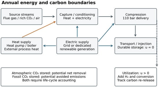
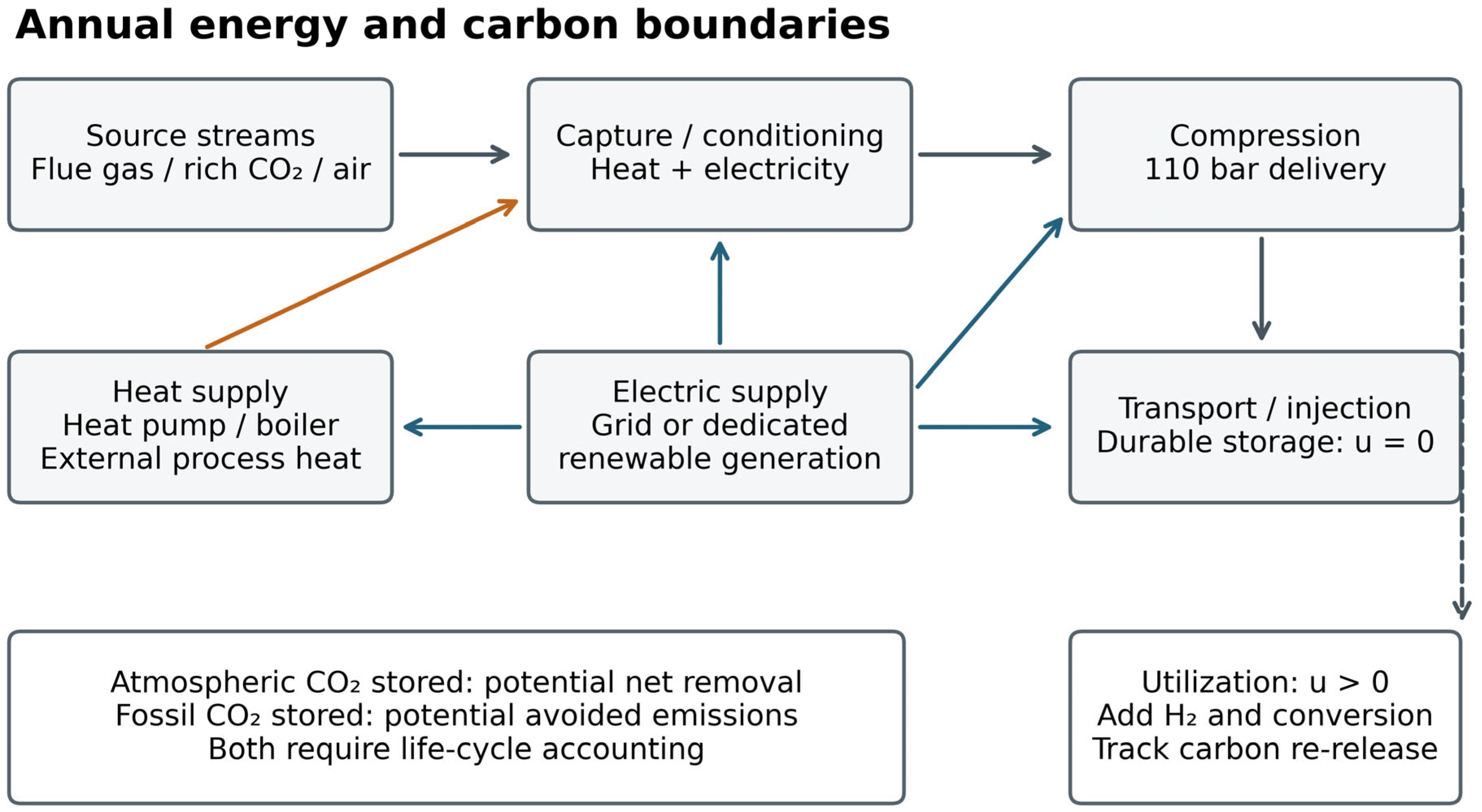
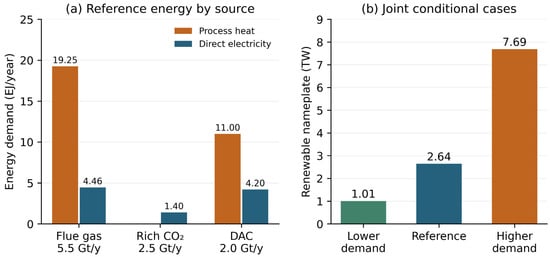
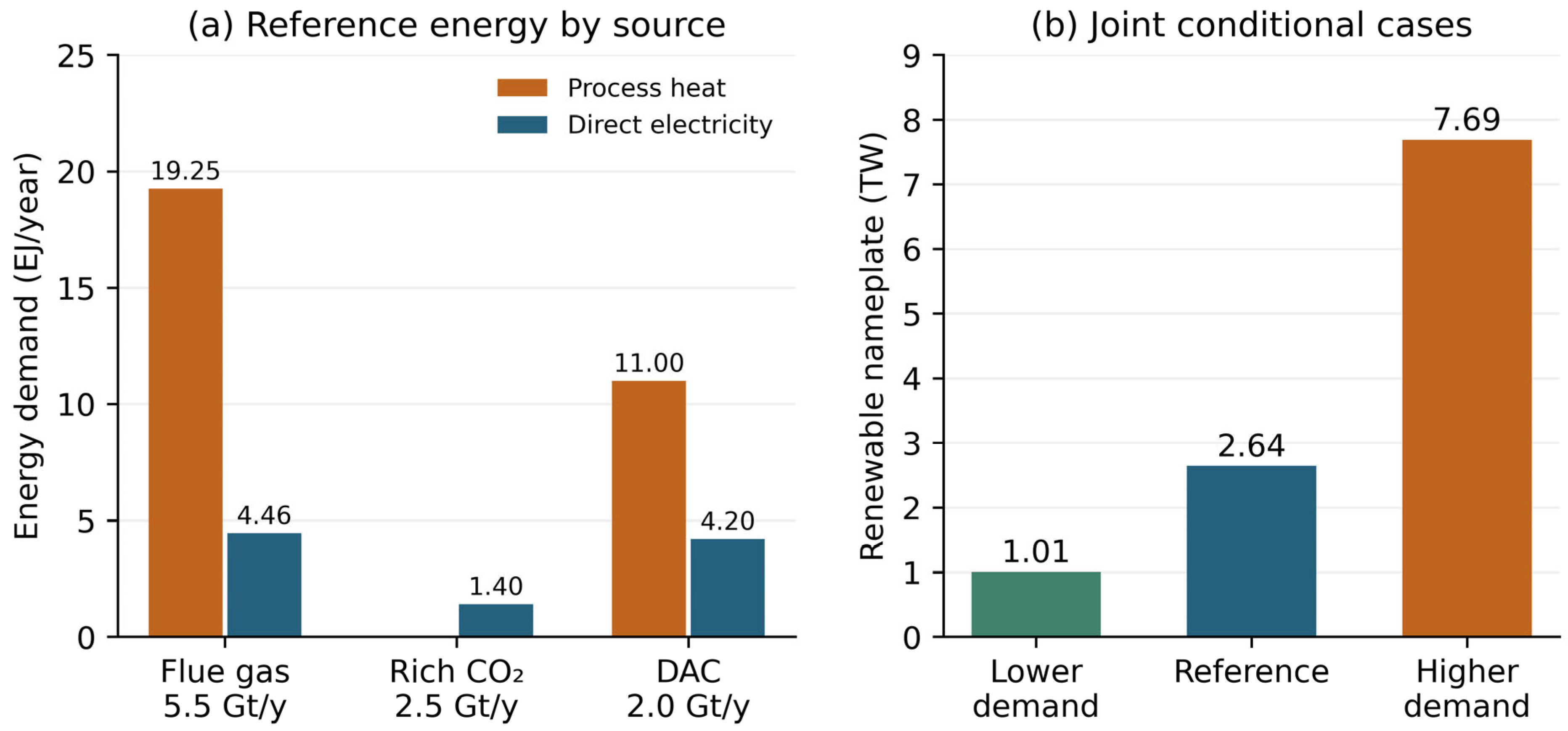
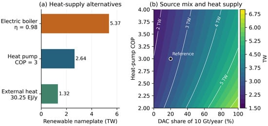
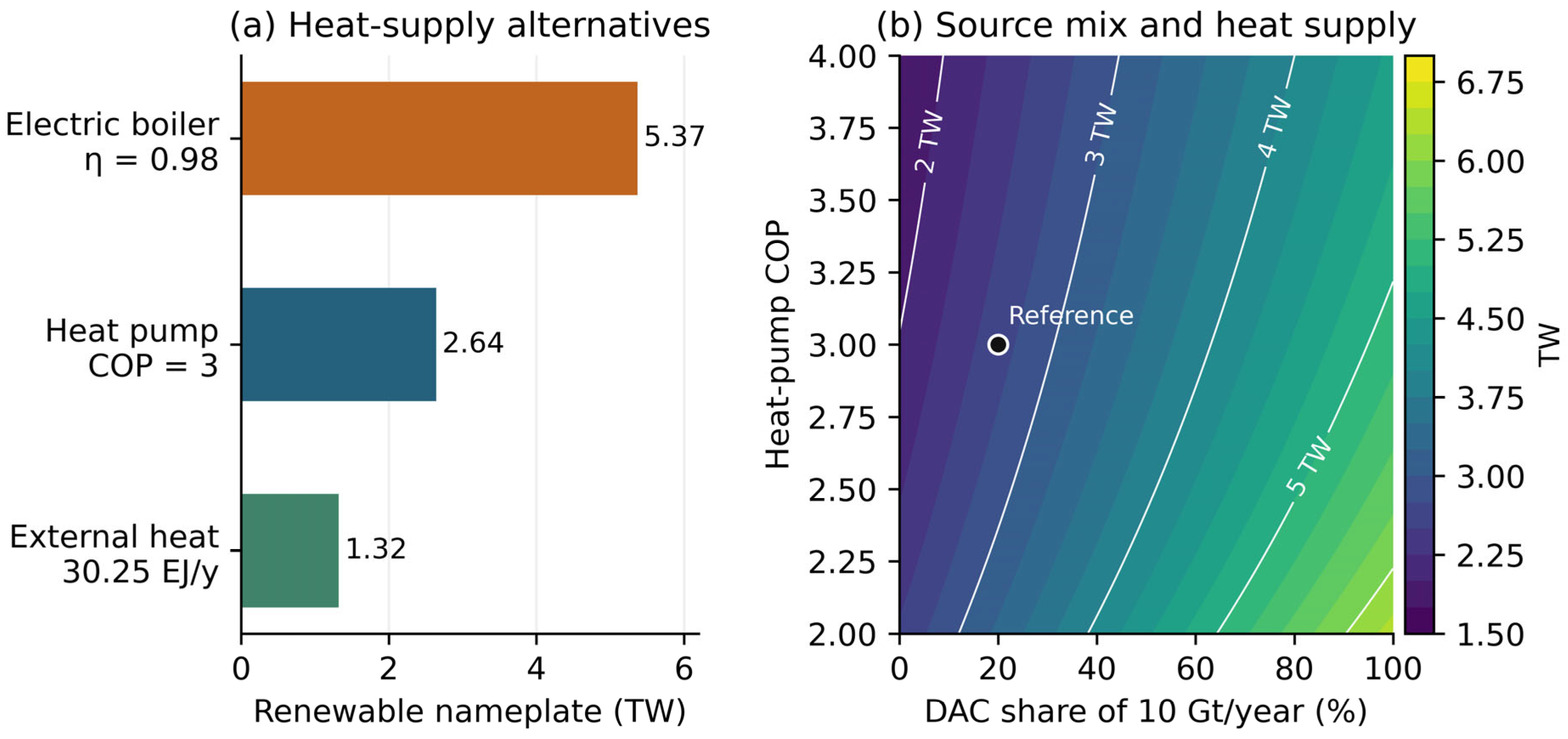
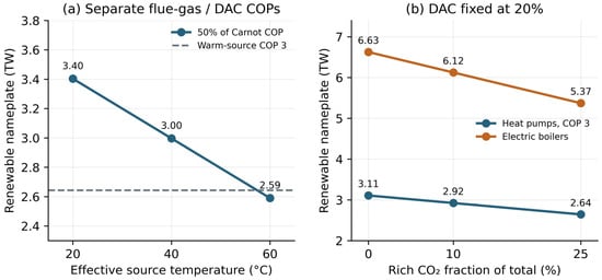
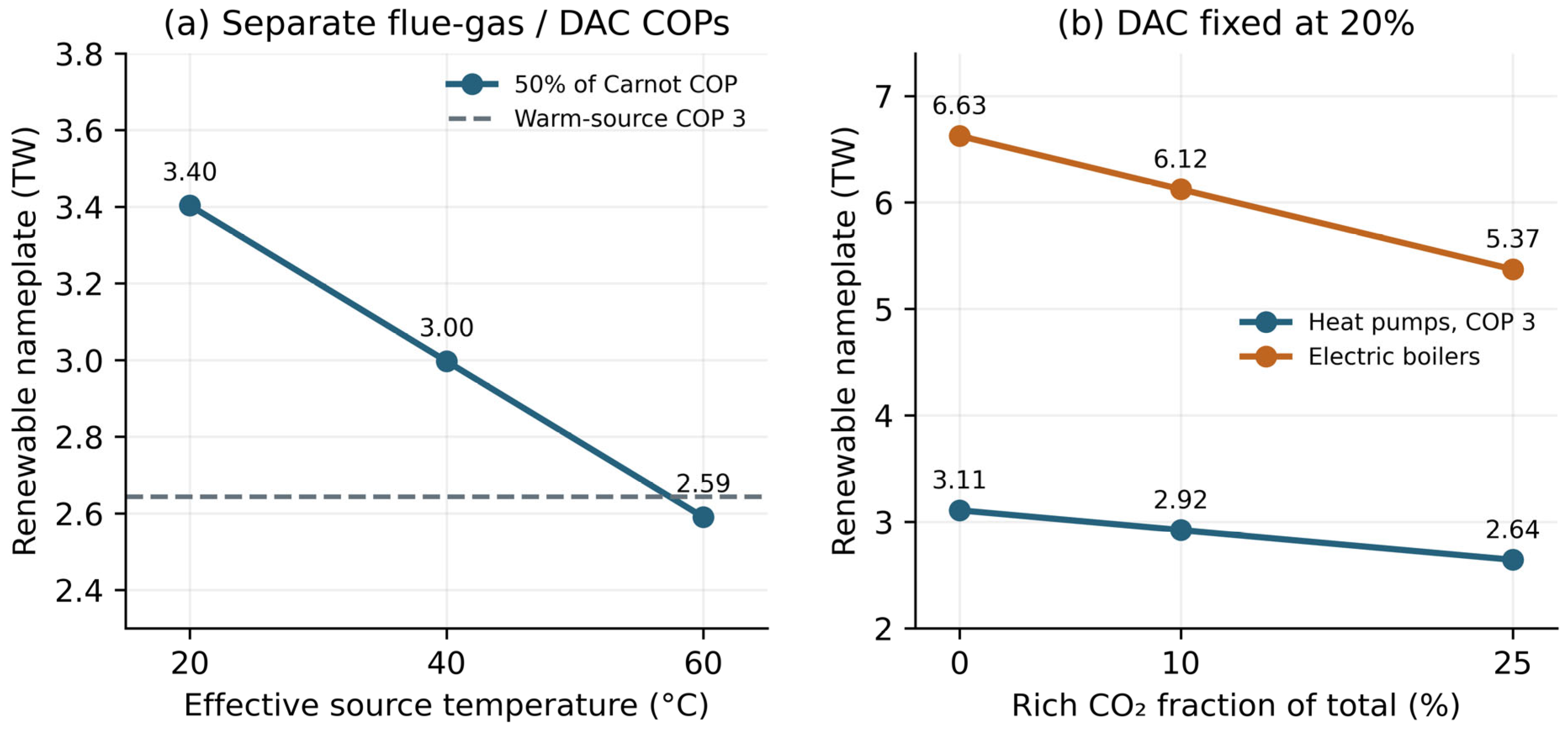
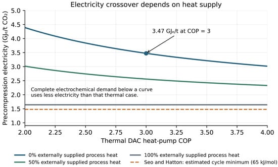
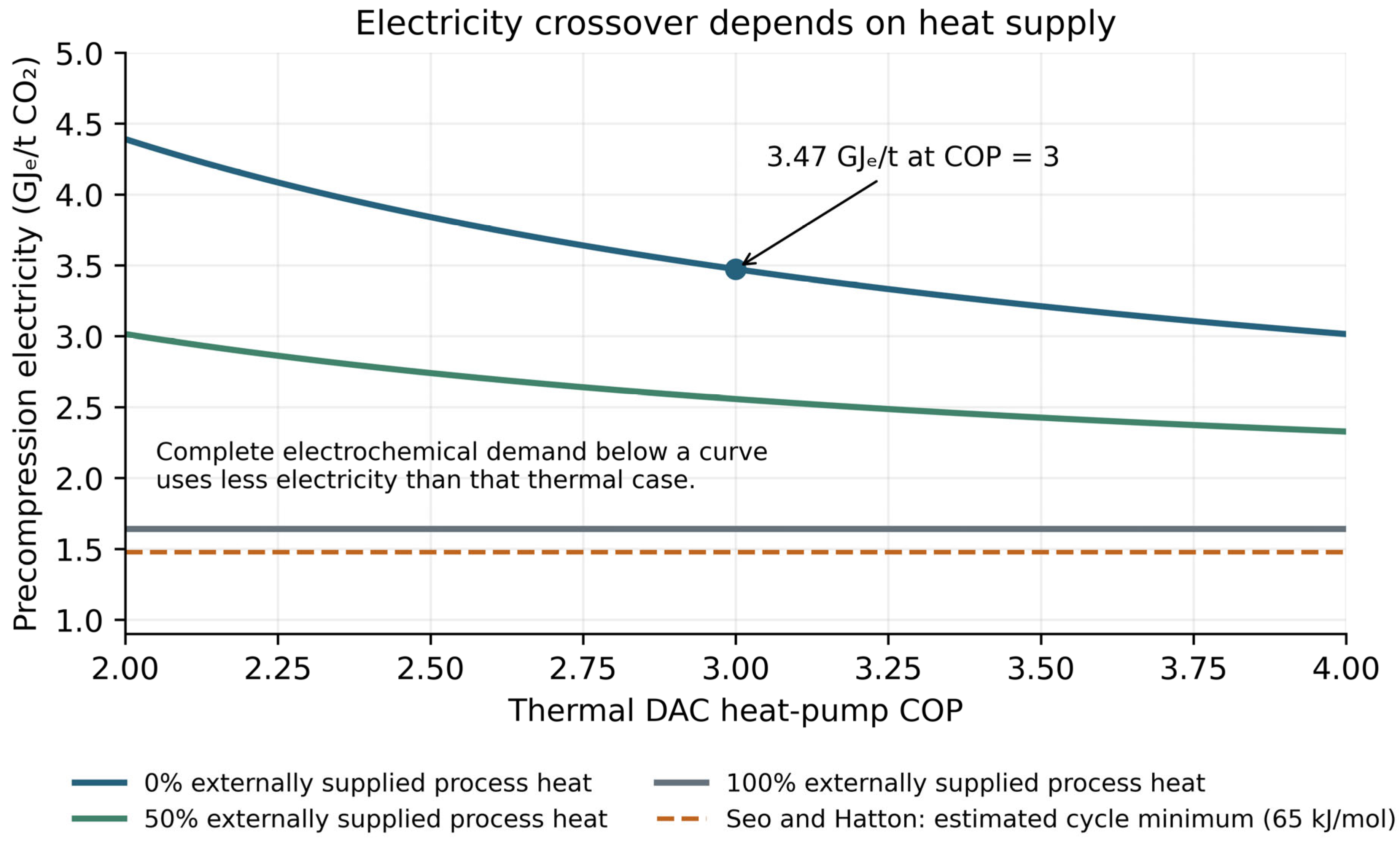
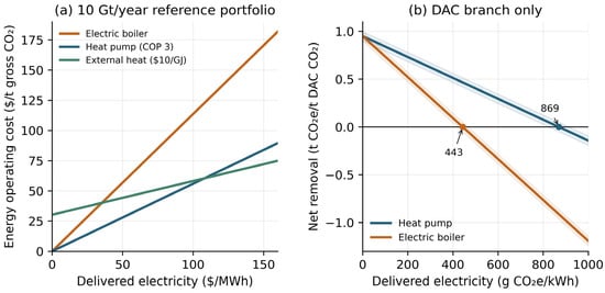
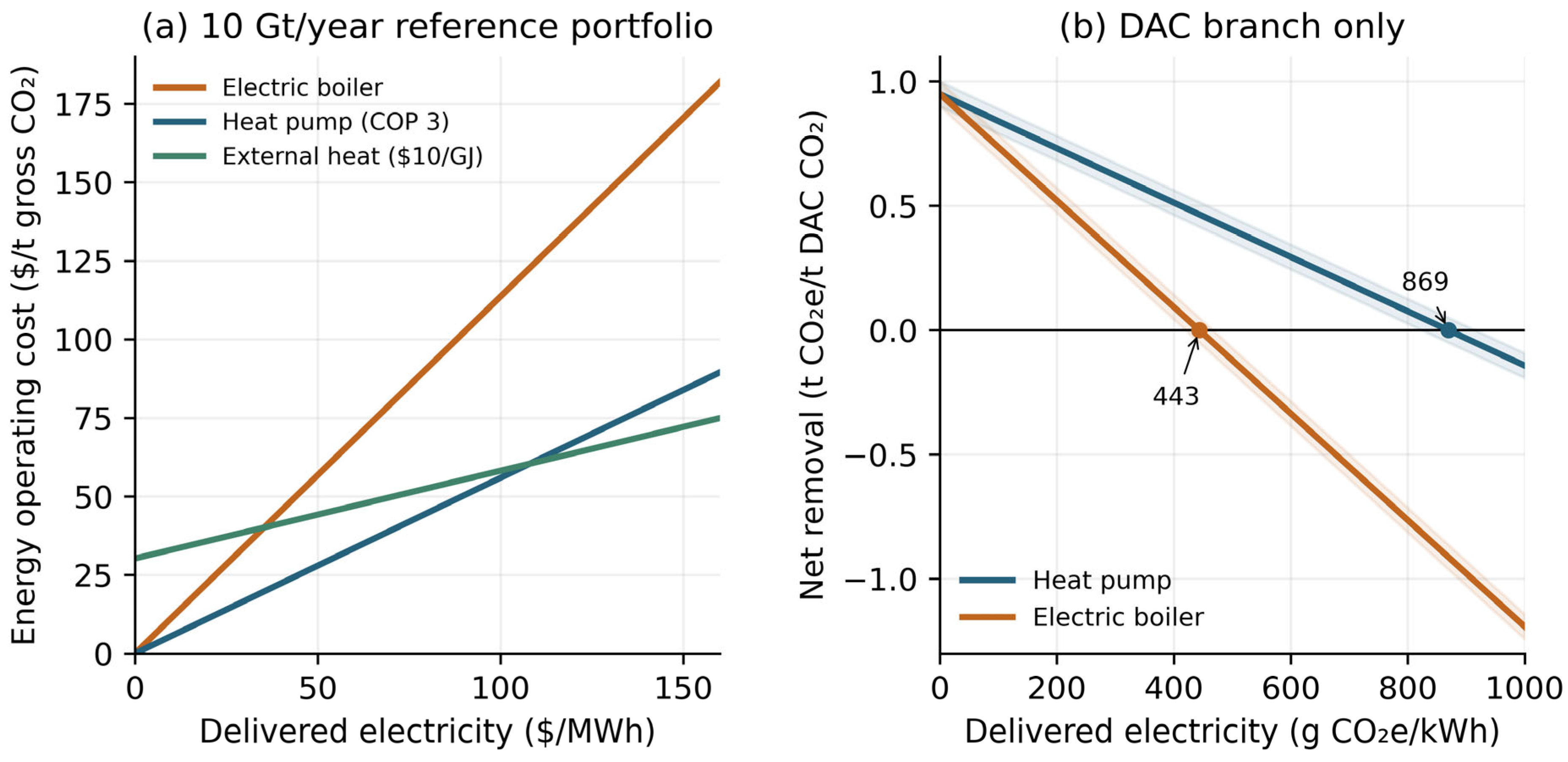
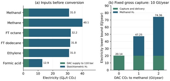
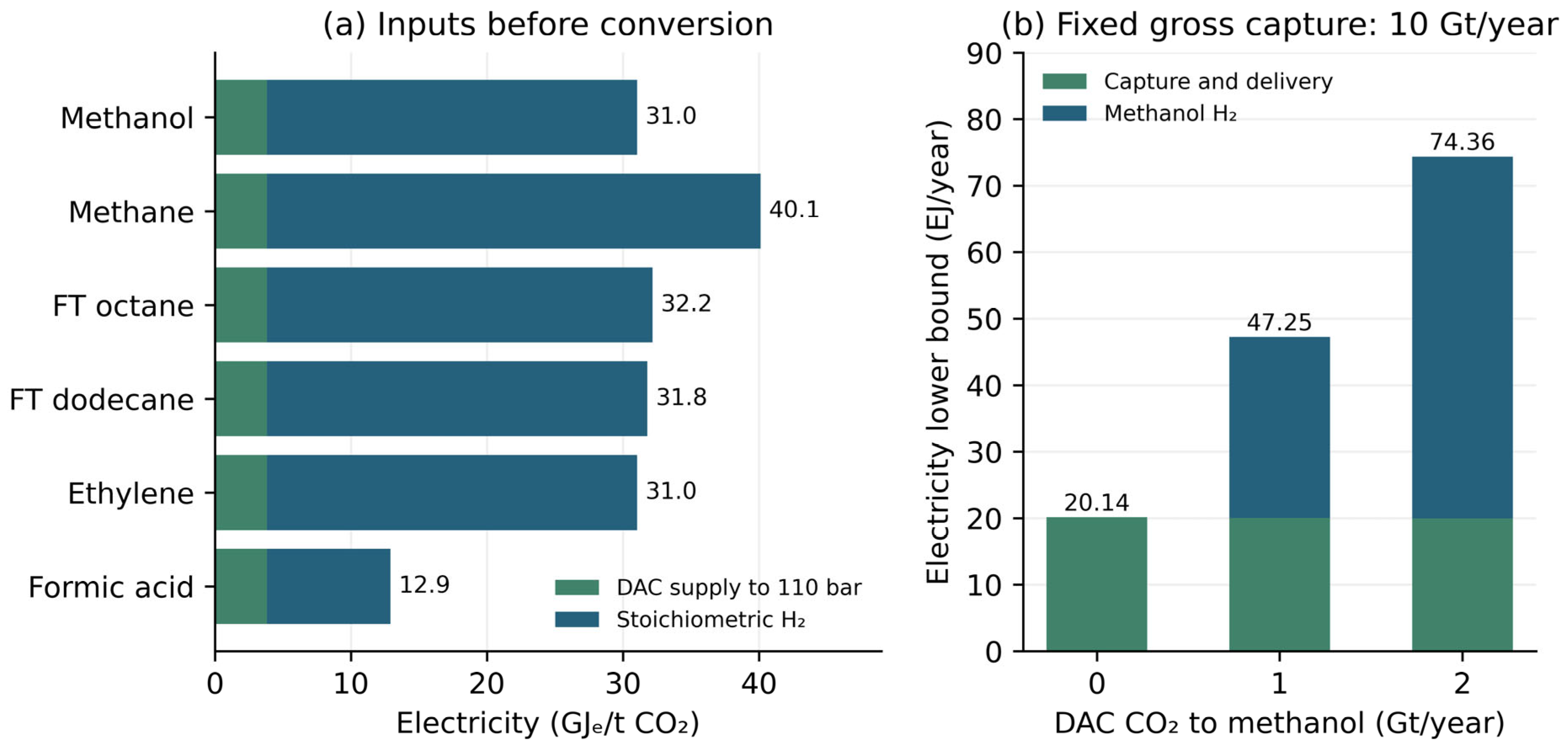
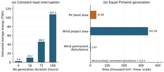
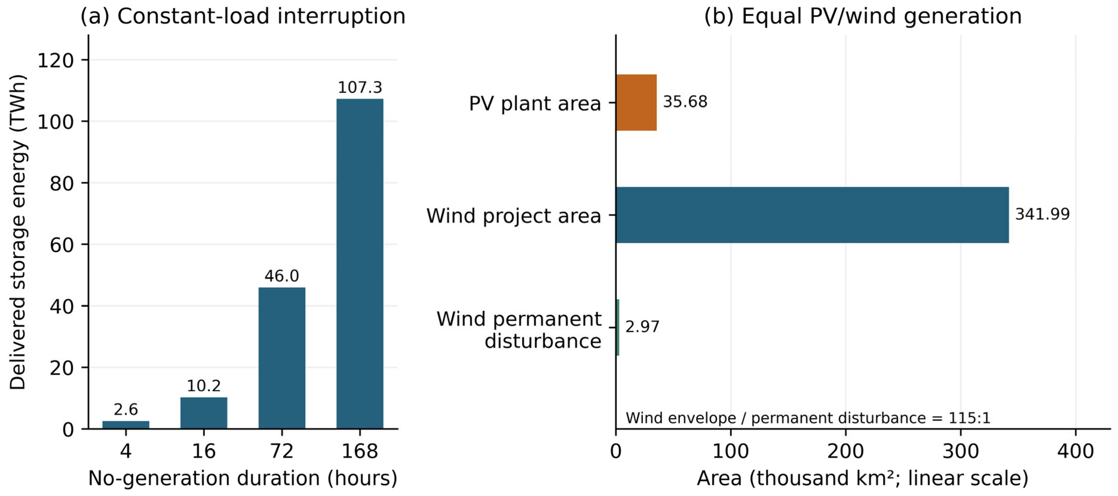

Disclaimer/Publisher’s Note: The statements, opinions and data contained in all publications are solely those of the individual author(s) and contributor(s) and not of MDPI and/or the editor(s). MDPI and/or the editor(s) disclaim responsibility for any injury to people or property resulting from any ideas, methods, instructions or products referred to in the content. |
© 2026 by the authors. Licensee MDPI, Basel, Switzerland. This article is an open access article distributed under the terms and conditions of the Creative Commons Attribution (CC BY) license.