


Abstract
This study compares four radial heat transfer models for buried oilfield gathering and transportation pipelines: DirectK, analytical thermal resistance, 1D FVM and 2D FVM, coupled with the same axial energy equation. Prescribed fluid properties and an internal heat transfer coefficient isolate the effects of radial model assumptions. After mesh, domain, boundary and transient checks, the 2D FVM is used as a numerical reference. Across 24 geometries, DirectK had a mean absolute relative heat-loss deviation of 32.5224%, whereas the maximum deviations of the analytical model and 1D FVM were 0.9344% and 0.9343%. Similar total heat losses did not imply identical local temperatures: the outer-surface top-to-bottom difference reached 6.8252 °C in the large-diameter, shallow-burial case. In case D, the 1D transient heat loss was 9.6510% lower than the 2D result at 168 h. The maximum startup temperature difference at 24 h was 0.2148 °C. Model selection therefore depends on the required temperature information, transient response and computational cost. These results are numerical comparisons under the stated assumptions, not field validation.
1. Introduction
The oilfield gathering and transportation pipelines are used to mix and convey crude oil, natural gas and associated water from wellheads to gathering facilities. During the transportation process, the fluid inside the pipeline exchanges heat with the surrounding soil and environment through the pipe wall, insulation layer and surrounding soil. This results in temperature changes along the pipeline. These temperature variations will alter the physical properties of the fluid and thereby affect the calculation results. Existing studies have coupled the pipe-soil heat transfer with axial flow and energy equations to calculate the fluid temperature and the temperature field of the surrounding medium in buried hot oil pipelines [1,2,3,4]. Dehdarinejad et al. [5] conducted experiments and numerical calculations to study heat loss from buried fuel oil pipelines under different flow conditions. Bossinov et al. [6] used on-site temperature data to validate oil temperature predictions under continuous operation and shutdown conditions. The heat transfer term in the axial energy equation is calculated using the radial heat transfer model, and the treatment of radial heat transfer will affect the temperature calculation results along the pipeline. Therefore, in the thermal analysis of gathering and transportation pipelines, an appropriate radial heat transfer model needs to be selected according to the specific calculation requirements.
The overall heat transfer coefficient method represents the convective heat transfer in the pipe, the heat conduction of the pipe structure layer, and the heat transfer of the soil using a fixed heat transfer coefficient. It requires fewer parameters and is suitable for calculations for long-distance pipelines and for multiple operating conditions. Zhou et al. [7] analyzed the relationship between operating parameters and the overall heat transfer coefficient. Their analysis indicates that factors such as flow rate, fluid properties, ambient temperature, pipe diameter, and wax deposition status all affect its value. Therefore, when the heat transfer coefficient determined under one operating condition is used for other operating conditions, the influence of pipeline structure, burial conditions, and changes in operating parameters needs to be considered.
Unlike the fixed overall heat transfer coefficient method, the analytical thermal resistance method separately calculates the thermal resistances of convection within the pipe, conduction through each structural layer, and conduction through the external soil. This determines the relationship between the fluid temperature and heat loss. For soil heat transfer under different boundary conditions, Thiyagarajan and Yovanovich [8] provided the thermal resistance expression for buried cylindrical bodies under constant heat flux boundary conditions. Bau and Sadhal [9] considered the coupling of heat transfer inside and outside the pipe, and derived the analytical solution for the heat loss of buried pipelines and the corresponding shape factor. Chung et al. [10] considered ground surface convective heat transfer and analyzed the soil temperature distribution and total heat transfer. Otomi et al. [11] provided the thermal resistance solution for steady-state heat transfer of the fully buried pipeline and analyzed the influence of burial depth. These studies provided a basis for calculating the soil thermal resistance under different burial depths and boundary conditions. Archer and O’Sullivan [12] compared the equivalent cylinder model with the half-space model and discussed the determination of the outer radius of the equivalent cylinder. This provided a basis for simplifying the soil domain. This paper adopts a multi-layer cylindrical analytical thermal resistance model, determines the thermal resistance of each part based on the pipe structure and material parameters, and calculates the heat loss by connecting the thermal resistances in series. However, this model does not include the heat storage terms of the pipe structure and the soil, and cannot directly describe the transient temperature changes after changes in operating conditions.
During the transient process, the changes in temperature and heat loss are not only affected by thermal resistance but also related to the pipeline structure and the heat storage of the surrounding medium. Chaczykowski [13] found that in the transient conditions of the investigated natural gas pipelines, using the steady-state heat transfer term would overestimate the amplitude of temperature fluctuations. Wei et al. [14] discovered in a study of hot oil pipeline shutdown and restart that the temperature change in the surrounding soil lags behind that of the fluid inside the pipe. Wei et al. [15] also observed a lag in the soil thermal response in their study of reverse transport. Chen et al. [16] analyzed the lag and attenuation of the temperature response along the pipeline during non-isothermal batch transportation at a constant flow rate. Thus, the comparison of steady-state heat loss cannot replace the transient response analysis. The one-dimensional radial model retains the heat storage term in each material layer, which allows the model to calculate the changes in temperature and heat loss over time. However, due to the assumption of uniform circumferential temperature, it cannot provide the temperature differences at different circumferential positions.
The two-dimensional pipe-soil cross-sectional model can take into account the influence of the ground surface and describe the heat conduction processes above, below and on both sides of the pipe. Yuan et al. [4] calculated the heat transfer term using the overall heat transfer coefficient and the temperature field of the pipe wall and soil. They compared the temperatures along the pipeline under different pipe parameters and soil temperature conditions. The results showed that in a non-uniform natural soil temperature field, the selection of the environmental reference temperature in the one-dimensional model would affect the calculation results. Therefore, when comparing different models, the treatment of the external boundary also needs to be considered. Oosterkamp et al. [17] compared the results of one-dimensional and two-dimensional heat transfer calculations with experimental measurements. They demonstrated that the simplification of ground surface boundary conditions would affect the prediction of soil temperature and the heat exchange between the pipeline and the environment. In the field of multidimensional heat transfer modeling, Xie et al. [18] incorporated heat conduction through the wax layer into the three-dimensional temperature field calculation for buried pipelines. Yuan et al. [19] employed a cross-dimensional model to couple the restart process within the pipe with the time-varying soil temperature field. On the other hand, the two-dimensional calculation results are also affected by the computational domain and the discretization method. Xie et al. [20] analyzed the influence of the shape and range of the soil computational domain on the thermal calculation of buried pipelines. They indicated that the suitability of the computational domain and grid settings still needs to be verified in two-dimensional calculations.
To enhance the efficiency of numerical calculation for heat transfer in pipelines, previous studies have adopted data-based reduced-order models, dynamic thermal networks, and proper orthogonal decomposition–backpropagation (POD-BP) models to reduce the computational load [21,22,23]. Yu et al. [24] established a POD–Galerkin reduced-order model for buried hot oil pipelines. They applied it to transient thermal calculations during batch transportation and startup processes. For buried crude oil pipelines, Jiang et al. [25] combined mechanistic equations with data-driven methods to predict the transient soil temperature field. Li et al. [26] used neural networks to rapidly predict the oil temperature and the temperature field of the surrounding medium during pipeline shutdown. Besides computational efficiency, the models should also be compared in terms of their required inputs and the outputs they provide. Yan et al. [27] further employed Fourier neural operators and U-shaped networks to rapidly predict the steady-state oil temperature in buried hot oil pipelines. They also predicted the temperature fields of the surrounding media. Wieland et al. [28] compared the methods for calculating heat loss in buried heating pipelines and simultaneously examined the input parameters, the obtainable results, and the deviations between the methods. For gathering and transportation pipelines, even if different models predict similar steady-state heat losses, their local temperatures and transient responses may still be different. Therefore, based on the existing research, this paper further compares the local temperature, transient response, and temperature along the pipeline calculated by each model. It verifies the computational settings through checks of the grids, computational domains, and time steps to assess the influence of these settings on the model comparison results. It also analyzes the influence of radial heat transfer differences on the temperature along the pipeline. This is to provide a basis for model selection.
Based on the above issues, this paper uses a homogeneous flow model to describe the fluid in the pipe and establishes a two-dimensional pipe–soil cross-sectional finite volume model. It compares this model with the fixed overall heat transfer coefficient model, the multilayer cylindrical analytical thermal resistance model, and the one-dimensional radial finite volume model. Considering that the two-dimensional model can more completely describe the cross-sectional heat transfer process, this paper uses its calculation results as the reference. It focuses on examining whether similarity in steady-state total heat loss implies consistency in local temperature distributions and transient responses. It also considers computational cost when evaluating the applicability of the four radial heat transfer models. The selected models are limited to the pipe structure, physical properties, and boundary conditions examined in this paper. They do not consider interphase slip, flow pattern changes, or wax deposition processes. Each model adopts the same pipe structure and material thermal properties, uses the same heat transfer area basis, and processes the boundary conditions according to its respective assumptions. Firstly, the steady-state heat loss, material interface temperature, and circumferential temperature distribution are compared. Then, the heat loss response after a sudden change in fluid temperature is analyzed. Subsequently, the heat loss per unit pipe length of each model is introduced into the axial energy equation, and the temperature along the pipeline is compared using the same flow rate and fluid thermal properties for all models. The applicable conditions of each model are discussed based on the calculation results for different pipe diameters, relative burial depths, and heat transfer times, together with the calculation time.
2. Heat Transfer Model and Numerical Solution
This section presents the axial energy equation and the solution methods used for the radial models. It focuses on introducing the boundary conditions, meshing, and finite volume discretization of the two-dimensional pipe-soil cross-sectional model. Finally, it explains the coupled solution process for the axial and radial models.
2.1. Basic Assumptions of the Model
The pipeline studied in this paper is composed of a steel pipe, a polyurethane (PU) insulation layer and a polyethylene (PE) protective layer. The surrounding medium is soil. Each model uses the cross-sectional mean fluid temperature. Solid materials are regarded as homogeneous and isotropic media, and the thermal properties of the materials remain unchanged in all cases. The interface between adjacent materials satisfies the condition of continuous heat flux. The contact thermal resistance, as well as the axial heat conduction of the pipeline structure and the soil, is ignored. This study does not consider the effects of interphase slip, flow pattern changes, wax deposition, or non-Newtonian rheology on heat transfer inside the pipe and thermal resistance.
This paper compares the two-dimensional pipe-soil cross-sectional finite volume model (2D FVM), the direct overall heat transfer coefficient model (DirectK), the multi-layer cylindrical analytical thermal resistance model, and the one-dimensional radial finite volume model (1D FVM). The main differences among the four models lie in the calculation methods of the overall heat transfer relationship, the treatment of the soil domain, and whether heat storage and circumferential temperature variations are considered. See Table 1.
Table 1.
Main differences among four types of radial heat transfer models.
These four types of models are all used for comparing steady-state heat losses. The material interface temperature and radial temperature distribution are compared between the analytical thermal resistance model and the two FVMs. The circumferential temperature difference is calculated by the 2D FVM. The transient part focuses on comparing the heat loss responses of the two FVMs. It uses the steady-state results of DirectK and the analytical thermal resistance model under the same boundary conditions as a reference to analyze the impact of heat storage on the heat transfer process.
2.2. Axial Energy Equation
The fluid is represented as a single equivalent thermal continuum with a uniform cross-sectional mean temperature. Flow rate and effective fluid properties are prescribed rather than obtained from a phase-resolved hydraulic calculation. If mixture properties are supplied, gas and liquid are assumed to share pressure, velocity and temperature, and volume and mass weighting give the following density and specific heat capacity, respectively:
Here, αg and αl are the gas and liquid volume fractions, dimensionless; ρg, ρl and ρm are the gas, liquid and effective-fluid densities, kg/m3; and cp,g, cp,l and cp,m are their specific heat capacities at constant pressure, J/(kg·K). Subscripts g, l and m denote gas, liquid and the equivalent mixture, respectively. Equation (1) defines optional effective thermal properties and does not constitute a phase-resolved flow model.
In the radial comparison cases, different radial models use the same constant values of mass flow rate, mixture density, specific heat capacity at constant pressure, and the internal pipe heat transfer coefficient. This allows the influence of radial heat transfer treatment methods to be compared.
The axial heat conduction of the fluid is ignored, and the heat loss per unit pipe length calculated by the radial model is substituted into the axial energy equation:
Here, Af is the flow cross-sectional area, m2; hm is the fluid specific enthalpy, J/kg; is the mass flow rate, kg/s; x is the axial coordinate in Equation (2), m; t is time, s; and q’ is heat loss from the fluid to the pipe wall per unit pipe length, W/m. For a circular pipe, Af = πDi2/4, where Di is the pipe inner diameter, m. For the constant-property comparison cases, temperature is recovered from enthalpy using the prescribed constant specific heat capacity.
The q′ values calculated for each radial model are respectively substituted into the same axial energy equation to obtain the corresponding temperature of the fluid along the pipeline. The inlet fluid temperature is given, and a natural outflow condition is applied at the outlet. For transient calculations, the given temperature distribution inside the pipe is used as the initial condition.
2.3. Simplified Radial Model
Both DirectK and the analytical thermal resistance model calculate the heat loss based on the steady-state heat transfer relationship, without considering radial heat storage. The 1D FVM retains the heat storage term and calculates the temperature field and heat loss by solving the radial heat conduction equation.
2.3.1. Steady-State Thermal Resistance Model
Each model calculates the heat loss at the inner wall of the pipe and uses the same heat transfer area as the reference. The heat transfer rate through the inner wall per unit pipe length is denoted by q′ (W/m). The direction of heat transfer from the fluid to the pipe wall is taken as positive. When using the overall heat transfer coefficient, the heat transfer relationship is:
q’ = KbπDb(Tf − Ta)
Here, Kb is the overall heat transfer coefficient based on reference diameter Db, W/(m2·K); Db is that diameter, m; Tf is the cross-sectional mean fluid temperature, °C; and Ta is the ambient reference temperature, °C. Only temperature differences enter the heat-loss relation.
The heat loss of DirectK is calculated according to Equation (3). Based on the inner wall area of the pipe, the overall heat transfer coefficient is calculated from the reference heat loss obtained using the method of images:
Here, Ki is the coefficient based on the pipe inner-wall area, W/(m2·K); q’ref,0 is the method-of-images heat loss at the calibration condition, W/m; Di,0 is the calibration inner diameter, m; and Tf,0 and Ta,0 are its fluid and ambient temperatures, °C. Subscript 0 denotes the calibration condition.
The analytical thermal resistance model is based on the current pipe structure and material parameters. The convective resistance within the pipe, the thermal resistance of the structural layer, and the thermal resistance of the soil are calculated separately. Then, these resistances are connected in series to obtain the total thermal resistance per unit pipe length and the heat loss:
Here, Rtotal and Rsoil are the total and soil thermal resistances per unit pipe length, m·K/W; hi is the internal convective heat transfer coefficient, W/(m2·K); Dj,o and Dj,i are the outer and inner diameters of structural layer j, m; λj is its thermal conductivity, W/(m·K); and q’ana is analytical-model heat loss per unit pipe length, W/m. Index j runs over the solid pipe layers.
Under the condition of a constant-temperature ground surface, the soil thermal resistance is expressed by the method-of-images analytical formula:
Here, H is the vertical distance from the pipe centerline to the ground surface, m; Dout is the complete outside diameter including the insulation and PE layers, m; λs is the soil thermal conductivity, W/(m·K); and arcosh is the inverse hyperbolic cosine.
2.3.2. One-Dimensional Transient Heat Conduction Model
The 1D FVM treats the surrounding soil as a cylindrical layer with an inner radius of re = Dout/2 and an outer radius equal to the pipe center burial depth H. The unsteady heat conduction equations for each structural layer of the pipe and the equivalent soil layer are:
Here, r is the radial coordinate from the pipe centerline, m; Tj is the temperature in material region j, °C; ρj is its density, kg/m3; and cp,j is its specific heat capacity, J/(kg·K). The soil-cylinder inner radius re = Dout/2, m.
The thermal conductivity and specific heat capacity of the equivalent soil layer are:
Here, λs,eq is the equivalent soil conductivity, W/(m·K); ρs,eq and ρs are the equivalent and original soil densities, kg/m3; and cp,s,eq and cp,s are the corresponding specific heat capacities, J/(kg·K). Subscript eq denotes the equivalent cylindrical soil representation.
The equivalent soil thermal conductivity is determined by Equation (8), so that the thermal resistance of the cylindrical layer is equal to the analytical value in Equation (6). The soil density remains unchanged, and the specific heat capacity and thermal conductivity are adjusted in the same proportion to keep the thermal diffusivity constant. However, it also excludes some lateral and deep soil regions, altering the volume of soil involved in heat storage and its spatial distribution. Therefore, its transient response may still differ from that of the two-dimensional model.
Convective boundary conditions are imposed at the pipe inner wall and the outer boundary of the equivalent soil layer, and temperature and normal heat flux are continuous across adjacent material interfaces:
Here, λst is steel thermal conductivity, W/(m·K); Tiw is the inner-wall temperature, °C; TH is the temperature at the cylinder outer radius r = H, °C; and ho is the outer-boundary heat transfer coefficient, W/(m2·K). The radial coordinate is positive outward from the pipe centerline.
The numerical example adopts a convective boundary at r = H. The ambient temperature is given according to the operating conditions, and the heat transfer coefficient is set at 108 W/(m2·K), approximating a constant-temperature condition.
Control volumes are defined along the radial direction, and the heat conduction equation is discretized using the finite volume method. The thermal conductivity of the shared face is taken as the distance-weighted harmonic average, and the transient term is discretized using the fully implicit scheme. With the given temperature field as the initial condition, the inner wall temperature is solved for at each time step, and the heat loss per unit pipe length is calculated:
q‘1D(t) = hiπDi[Tf(t) − Tiw(t)].
Here, q’1D is the full-circumference heat loss per unit pipe length predicted by the 1D FVM, W/m.
2.4. Two-Dimensional Cross-Sectional Heat Transfer Model
2.4.1. Computational Domain and Governing Equations
The computational domain of the two-dimensional model includes the steel pipe, insulation layer, PE protective layer and the surrounding soil. The horizontal and vertical coordinates of the cross-section are denoted as x and y, respectively. The ground surface is at y = 0, and the center of the pipeline is at (0, −H).
A finite rectangular soil domain around the pipeline is selected as the computational domain. If the geometry, material distribution and boundary conditions are all symmetrical about the vertical centerline of the pipeline, only the right half domain (x ≥ 0) is calculated. The width and depth of the computational domain are denoted as Wdom and Ddom, respectively.
Here, Wdom is the distance from the symmetry plane to the right boundary, m, and Ddom is the depth below the ground surface, m. The selected dimensions are Wdom = 8 max(4H, 6Dout) and Ddom = 8 max(5H, H + 6Dout). During domain enlargement, the pipe, material interfaces and near-field cells remain unchanged; only the soil mesh at the sides and bottom is extended. Domain checks are reported in Appendix B.4. The material regions and boundaries are shown in Figure 1.
Figure 1.
Two-dimensional pipe-soil computational domain and boundary conditions. ho denotes the ground-surface heat transfer coefficient. The orange-red, gray, yellow, and green regions represent the fluid, steel pipe wall, PU insulation, and PE protective layer, respectively. The pale-yellow background denotes the computed soil half-domain, while the faded left half illustrates the uncomputed symmetric counterpart.
The same form of two-dimensional heat conduction equation is adopted in each material region:
Here, x and y are the horizontal and vertical coordinates of the two-dimensional cross-section, m. The cross-sectional x is distinct from the axial coordinate used in Equation (2); y = 0 is the ground surface and the pipe center is at (0, −H).
2.4.2. Boundary Conditions
Adjacent materials exchange heat through a common interface. When the contact thermal resistance is ignored, the temperatures on both sides of the interface are equal, and the normal heat flux is continuous.
Tj = Tk, λj∇Tj ⋅ njk = λk∇Tk ⋅ njk.
Here, j and k identify adjacent material regions; njk is the unit normal pointing from region j to region k, dimensionless; and ∇ denotes the spatial gradient operator. The same normal direction is used on both sides of the interface.
In the model comparison case, convective heat transfer boundary conditions are applied at the inner wall of the pipe and the ground surface. The heat transfer coefficient within the pipe is set to 300 W/(m2·K). For the ground surface, it is set to 108 W/(m2·K) to approximate a constant-temperature ground surface boundary condition. The temperature at the bottom boundary of the soil is specified. Zero normal heat flux conditions are applied at the far-side boundary and the symmetry plane.
Here, Tw is the local inner-wall temperature, °C; Ts is soil temperature, °C; Tdeep is the prescribed bottom-boundary temperature, °C; nr points radially from the fluid into the solid, while n is the outward normal on an external boundary. Both normals are dimensionless. Γi, Γs, Γb, Γsym and Γside denote the inner wall, ground surface, bottom, symmetry and far-side boundaries, respectively.
To characterize the relative influence of surface convection and soil heat conduction, the surface Biot number is defined using the pipe centerline burial depth H as the characteristic length:
Here, Bis is the surface Biot number, dimensionless. The definitions and units of ho, H and λs are given above. For the 24 geometries in Section 4.2.1, Bis ≥ 107, consistent with the approximately constant-temperature ground boundary used here. This number characterizes the external boundary condition only.
2.4.3. Grid and Equation Discretization
The steel pipes, insulation layer, PE protective layer and the soil near the pipes are all covered by a conformal quadrilateral grid. The surrounding soil is covered by a Delaunay triangular grid, with the grid density increasing closer to the pipes. Each material region is discretized into grid cells, and the heat conduction between areas is calculated through the shared faces. The overall grid and the local grid near the pipes are shown in Figure 2.
Figure 2.
Selected pipe–soil mixed mesh: (a) Cropped near-field view, mirrored only for display; (b) Local pipe-layer detail. The full benchmark right half-domain is 48 m wide and 60 m deep and extends beyond the crop. PU, polyurethane; PE, polyethylene.
The shared-face conductivity uses a distance-normalized harmonic average. For adjacent control volumes P and N sharing face f, the sum of the cell-center-to-face distances is used in the numerator:
Here, λf is the shared-face conductivity, W/(m·K); λP and λN are the conductivities of cells P and N, W/(m·K); and dPf and dNf are the respective cell-center-to-face distances used in the conductivity weighting, m. Symbols P, N and f identify the owner cell, neighboring cell and shared face.
Integrating the governing heat conduction equation over each control volume and discretizing the transient term using a fully implicit scheme gives:
Here, and are the new-time cell temperatures, °C; aP and aPN are the diagonal and neighbor coefficients per unit pipe length, W/(m·K); bP is the known-term contribution, W/m; and NB(P) is the set of neighbors of P. Superscripts n and n + 1 denote successive time levels.
The shared face flux in the discrete equation adopts a non-orthogonal correction form. The temperature gradient is calculated using the weighted least-squares method. The temperature at the material interface is calculated using thermal-resistance weighting. The heat conduction distance at the boundary is taken as the normal distance, and the effect of boundary grid skewness is corrected for. After obtaining the cross-sectional temperature field, the heat transfer rates of the inner-wall boundary segments in the right half domain are added together. The sum is then converted into the heat loss per unit length for the complete cross-section:
Here, q’2D is the heat loss per unit pipe length for the full cross-section, W/m; Nb is the number of inner-wall boundary segments in the computed half-domain, dimensionless; e is the segment index; Tw,e is its wall temperature, °C; and Le is its length, m. The factor 2 restores the complete circumference from the symmetric half-domain.
2.5. Coupled Axial–Radial Solution
The axial and radial models are coupled through the fluid temperature Tf and the heat loss q′ per unit pipe length. The fluid temperature of each axial control volume is used to determine the heat transfer boundary of the inner wall of the corresponding section. The heat loss calculated by the cross-sectional model is then substituted into the axial energy equation.
The pipe is divided into axial control volumes. The convective term is discretized using a first-order upwind scheme, and the transient term using a fully implicit scheme. For the forward flow, the discrete equation of the i-th control volume is:
Here, is the fluid mass in axial control volume i, kg; Δx is its axial length, m; Δt is the time step, s; n and n + 1 denote the old and new time levels; and i − 1 denotes the upstream control volume for forward flow. The subscript i on fluid properties indicates the local control-volume value. hm,i and q’i retain the specific-enthalpy and heat-loss definitions given above.
At steady state, the heat storage term of the fluid is ignored. Using i and i + 1 to represent the starting and ending points of the pipe section respectively, the temperature is calculated segment by segment along the flow direction:
Here, Tf,i and Tf,i+1 are the upstream and downstream temperatures of the steady segment i, °C; is its prescribed mass flow rate, kg/s; cp,m,i is its local fluid specific heat capacity, J/(kg·K); and q’i is the heat loss per unit pipe length of segment i, W/m, evaluated at the downstream temperature Tf,i+1.
For a transient step with constant properties and fixed heat transfer coefficients, the cross-sectional field from the previous time level is retained as the initial state. Two trial fluid temperatures determine the linear implicit heat-loss response, which is substituted into Equation (18) to solve for the new fluid temperature; the cross-sectional field is then updated and stored without an additional nonlinear iteration. Equation (19) is the corresponding steady segment relation. The axial–radial coupling is shown in Figure 3. The fixed-coefficient startup evaluation and its checks are described in Appendix B.5.
Figure 3.
Schematic diagram of axial-radial coupling calculation: (a) Pipeline and local thermal slices; (b) Axial discretization and thermal coupling. Blue arrows indicate axial flow, red arrows indicate heat loss to the surroundings, and green planes represent local thermal slices.
3. Evaluation Method for Radial Heat Transfer Model
3.1. Principles for Model Selection
The radial heat transfer of buried gathering and transportation pipelines includes heat exchange between the fluid and the inner wall of the pipeline, as well as heat conduction within the pipeline structure layer and in the surrounding soil. When calculating the steady-state temperature drop along the pipeline, the main requirement is the heat loss per unit length of the pipeline. When analyzing the temperatures at the top and bottom of the pipeline and in the adjacent soil, the cross-sectional temperature distribution is also needed. When simulating transient processes such as pipeline startup, it is also necessary to assess whether heat storage in the pipe structure and surrounding soil can be neglected. To meet these requirements, this paper compares the steady-state heat loss, local temperature, and transient response of each model, and analyzes the influence of radial heat transfer differences on axial temperature. The applicability of the models is discussed in conjunction with calculation deviations and computation time. The model selection approach is shown in Figure 4.
Figure 4.
Framework for selecting the radial heat transfer model.
3.2. Model Comparison Method
3.2.1. Comparison of Conditions and Definition of Heat Loss
In the same case study, all models use identical pipeline structures and material thermal properties. The pipeline geometric parameters include the inner diameter Di, outer diameter Do of the steel pipe, burial depth H from the pipe center to the ground surface, and the thickness of each structural layer. The relative burial depth is defined as H/Do, where Do does not include the insulation layer and the PE protective layer. When comparing different operating conditions, the thicknesses of the structural layers remain unchanged, while the burial depth is calculated based on Do and H/Do.
In the radial model comparison, each model adopts the same cross-sectional average fluid temperature and convective heat transfer coefficient inside the pipe. In the axial coupling comparison, the mass flow rate, fluid thermophysical properties, inlet and initial conditions, axial grids, and time step are all kept consistent. Each model uses the same external environmental conditions, but the soil domain and its outer boundary are handled according to the respective model assumptions. The equivalent thermal conductivity and specific heat capacity of the 1D FVM are obtained by converting the given soil thermophysical properties.
This article consistently takes the inner wall area of the pipe as the reference; that is, Db = Di. The overall heat transfer coefficient under other area references can be converted according to the following formula:
Here, subscripts 1 and 2 identify the original and converted area bases, respectively; Kb,1 and Kb,2 are overall heat transfer coefficients, W/(m2·K), and Db,1 and Db,2 are their reference diameters, m. During a transient, storage in the pipe layers and soil means that heat leaving the fluid generally differs from simultaneous heat leaving the soil outer boundary.
3.2.2. Evaluation Indicators
Under steady-state heat conduction conditions with a constant ground surface temperature and homogeneous soil, the calculation results of the 2D FVM are used as the reference. The absolute relative deviation of the steady-state heat loss is defined as:
Here, εq is the absolute relative heat-loss deviation, %; q’m is the heat loss of the model being compared, W/m; and q’2D is the 2D FVM reference heat loss, W/m. In this indicator, subscript m identifies a model, not the mixture-property subscript in Equation (1).
The mean and maximum heat-loss deviations and the number of cases with deviations exceeding 5% are reported, with 5% used as a statistical comparison threshold in this study. The thermal resistance model and the method-of-images analytical solution adopt the same expression for soil thermal resistance. The comparison between the two is mainly used to check the calculation implementation of the thermal resistance formula. The overall heat transfer coefficient of DirectK is determined by the reference heat loss of the reference working condition, so the heat loss predicted by DirectK equals the reference heat loss under that condition. The differences between the two FVMs and the analytical results are also affected by the simplification of the soil domain, boundary conditions, and discretization methods.
Local temperature comparisons include the temperature at the material interface and the temperature distributions above and below the pipe. Temperatures predicted by the models are compared at the pipe inner wall and at the outer surface of each structural layer. The two-dimensional model takes the circumferential average value at each interface and then compares it with the results of the analytical thermal resistance model and the 1D FVM. The circumferential temperature difference in the outermost surface of the pipeline is represented by the temperature difference between the top and bottom of the pipe:
ΔTub = |Ttop − Tbottom|
Here, ΔTub is the magnitude of the top-to-bottom temperature difference on the outermost pipe surface, °C; Ttop and Tbottom are the temperatures at its top and bottom, °C.
The circumferential temperature variations under different geometric conditions are compared using ΔTub = 1 °C as the screening value for the circumferential temperature difference. This indicator reflects the degree of nonuniformity in the circumferential temperature distribution. It is used to determine whether a two-dimensional model should be adopted for local temperature calculations. It is not related to wax precipitation, stress, or safety limits. The calculated results obtained correspond only to the operating conditions described in this article. In practical applications, the acceptable temperature difference should be determined based on specific requirements.
For the transient process after a sudden change in fluid temperature, the relative difference in heat loss between 1D FVM and 2D FVM is compared to evaluate the two models:
Here, δq is the signed relative difference in transient heat loss, %; q’1D(t) and q’2D(t) are the simultaneous full-circumference heat losses from the 1D and 2D FVMs, W/m.
Under the conditions of outward heat transfer from the fluid in this article, q’2D(t) > 0. When δq(t) is positive, the heat loss of the 1D FVM is higher; when it is negative, the heat loss of the 2D FVM is higher. After the calculation, the transient heat losses predicted by the two models are compared with their respective steady-state values, which serve as reference values.
Each radial model is coupled with the axial energy equation. The axial temperature difference is defined relative to the fluid temperature predicted using the 2D FVM:
ΔT2D(x,t) = Tmodel(x,t) − T2D FVM(x,t)
Here, ΔT2D is the signed axial fluid-temperature difference relative to the 2D-coupled result, °C; Tmodel and T2D FVM are the fluid temperatures predicted using the compared model and 2D FVM, °C; and x again denotes axial distance, m.
When the temperature difference is positive, the fluid temperature calculated by the model to be compared is higher than that of the 2D FVM. When it is negative, it is lower than that of the 2D FVM. The axial distribution of temperature differences, including the difference at the outlet, is examined to assess how the choice of radial model affects the predicted fluid temperature.
In the pipeline startup calculations, the arithmetic mean of the initial fluid temperature and the inlet temperature after startup is defined as the characteristic temperature:
Here, Tref is the characteristic front temperature, °C; Tinitial is the initial fluid temperature, °C; and Tin is the fluid inlet temperature after startup, °C.
The axial position where the fluid temperature reaches Tref is defined as the temperature front position. The temperature difference and the difference in the front position are used to compare the calculation results of the two models with the current axial grid and time step.
Radial evaluation and setup operations are timed separately. Table 11 reports only steady-state radial evaluation times; the timing scope is specified in Section 5.5. The solution times of each model under the same computing requirement are compared in conjunction with heat loss deviation, temperature distribution and transient response to provide a basis for model selection.
4. Numerical Verification and Case Setup
4.1. Numerical Verification
The radial heat transfer and axial temperature calculations were verified using the published steady-state case provided by Yuan et al. [4]. The absolute temperature difference at the outlet ranged from 0.0504 to 0.1184 °C. The relative difference in the temperature drop along the pipeline ranged from 0.4344% to 1.0202%. This recalculation retained the independent boundary conditions and axial solution settings, as detailed in Appendix A. The comparison of results is used only to check numerical consistency. The applicability of the model under actual conditions still requires validation against experimental or field data.
The selected 1D FVM uses 200 radial cells per layer and geometrically graded soil cells. The selected 2D FVM uses 48 radial cells per pipe layer and 288 equivalent circumferential cells over a full circle, corresponding to 144 cells in the computed right half-section, with soil size scale 0.5. Radial transient time steps are 30, 150 and 225 s. The mesh, domain, boundary and time-step checks are reported in Appendix B. Startup verification separately examines the full outlet-temperature history, representative axial profiles, paired model temperature differences and temperature-front positions.
4.2. Parameters and Operating Conditions
4.2.1. Radial Heat Transfer Cases
Radial comparison is conducted on buried pipelines composed of steel pipes, polyurethane insulation layers and PE protective layers. The reference parameters are shown in Table 2. The published calculation example is reproduced using the parameters listed in Appendix A, which are different from the calculation conditions of the benchmark case in this section.
Table 2.
Benchmark parameters for comparison of radial heat transfer models.
To compare the effects of pipe diameter and burial depth on steady-state heat transfer, the outer diameter Do of the steel pipe was set at 0.10, 0.30, 0.60 and 1.00 m. The relative burial depth H/Do was taken as 1.5, 2, 3, 5, 10 and 20. This resulted in a total of 24 sets of conditions. The thickness of each structural layer remained unchanged, and the inner diameter of the pipe, the outer diameter of the pipeline, and the absolute burial depth were determined according to the parameter combinations. DirectK used the overall heat transfer coefficient of the reference condition, which is 0.6755 W/(m2·K). The other models calculated the steady-state heat loss and local temperature based on the pipe diameter and burial depth of each condition. Since the thickness of each structural layer is fixed, a change in pipe diameter will also alter the thickness-to-diameter ratios of the structural layers. Therefore, when analyzing the influence of geometric conditions, it is necessary to consider both factors together. Moreover, its applicability under other operating conditions still needs further verification.
In the reference transient condition, the initial temperatures of the fluid within the pipe, each structural layer, and the surrounding soil were all 10 °C. The fluid temperature rose instantaneously from 10 °C to 80 °C and remained constant. The calculation was carried out until 168 h. The heat loss changed rapidly during the initial stage and decreased gradually thereafter. The time steps for the three periods of 0–2 h, 2–24 h, and 24–168 h were set at 30, 150, and 225 s respectively.
To compare transient responses under different geometric conditions, four sets of operating conditions are specified in Table 3. The initial and ambient temperatures for all cases are set at 20 °C, while the fluid temperature is raised to 80 °C. The simulations are carried out up to 720 h. Time steps of 30 s, 150 s, and 225 s are used for the periods 0–2 h, 2–24 h, and 24–720 h, respectively. Cases A and B, as well as C and D, are used to compare the effects of relative burial depth at the same pipe diameter. Cases A and C, as well as B and D, are used to examine the influence of pipe diameter at the same relative burial depth.
Table 3.
Geometric conditions for radial transient comparison.
The above radial example retains the reference material parameters and boundary conditions, and the temperature conditions are specified separately for each working condition. The size of the two-dimensional computational domain is determined according to Section 2.4.1. For condition C, a right half domain with a width of 320 m and a depth of 400 m is adopted. When expanding the computational domain, keep the pipeline and the near-field grid unchanged.
To describe the above geometry and time scale, define the insulation layer thickness-to-diameter ratio ηins and the soil Fourier number Fos as follows:
Here, ηins is the insulation-thickness-to-steel-diameter ratio, dimensionless; δins is the insulation thickness, m; Fos is the soil Fourier number, dimensionless; αs is the soil thermal diffusivity, m2/s; and is the soil volumetric heat capacity, J/(m3·K). The pipe centerline burial depth H is the diffusion length scale. Table 2 gives αs = 7.5 × 10⁻⁷ m2/s. The 24 geometries span ηins = 0.0500–0.5000. These quantities characterize the investigated geometries and diffusion time scales; they do not establish a universal applicability boundary.
4.2.2. Axial Heat Transfer Cases
In the axial temperature comparison, for the same calculation case, each model uses the same mass flow rate and fluid thermal properties, and substitutes its respective radial heat loss into the axial energy equation. In the steady-state calculation case, the pipe length is 10 km, and 200 control volumes are defined along the axial direction. The inlet temperature is 90 °C, the ambient temperature is 10 °C, and the specific heat capacity of the fluid at constant pressure is 2200 J/(kg·K). The mass flow rates are respectively set at 5, 20, and 50 kg/s. The pipe structure, external heat transfer conditions, and local two-dimensional computational domains were the same as those used in the reference case.
The pipeline startup calculation couples the 1D FVM and 2D FVM with the same axial energy equation. The pipe length is 10 km, and the calculation is carried out up to 24 h. The effects of the axial grid and time step on the pipeline startup results are examined separately. The specific settings and verification results can be found in Appendix B.5. The mass flow rate, fluid density, and specific heat capacity at constant pressure are set at 10 kg/s, 850 kg/m3, and 2200 J/(kg·K), respectively, and remain unchanged. The initial temperatures of the fluid, pipe structural layers, and soil are all 10 °C. After the start-up, the inlet temperature rises to 80 °C and remains constant. The pipe structure, material thermal properties, and external boundary conditions are the same as the radial reference condition. The heat transfer coefficient inside the pipe is set at 300 W/(m2·K). The temperatures along the pipeline at 2, 6, 12, and 24 h are compared, and 45 °C is used to define the temperature front.
5. Results and Discussion
5.1. Steady-State Heat Loss
The heat loss per unit pipe length for each model under the reference condition is shown in Table 4. The overall heat transfer coefficient of DirectK is calibrated by the method-of-images analytical heat loss of this condition, so its calculated value is equal to the reference value. The analytical thermal resistance model uses the same expression for soil thermal resistance, and the results are also close to the reference value. With the 2D FVM results as the reference, the absolute relative deviations for DirectK and the analytical thermal resistance model are both 0.0472%. The corresponding deviation for the 1D FVM is 0.0469%. All four models predicted similar heat loss per unit pipe length under the reference condition.
Table 4.
Steady-state heat loss under base conditions.
Figure 5 and Table 5 present the comparison results for the steady-state heat loss of each model under 24 combinations of pipe diameter and relative burial depth. The 2D FVM results are used as the reference. The average absolute relative deviations for the analytical thermal resistance model and the 1D FVM are 0.2420% and 0.2414%, respectively. The maximum absolute relative deviations are 0.9344% and 0.9343%, respectively. Within the geometric range under investigation, the steady-state heat losses calculated by these two simplified models are close to those calculated by the 2D FVM.
Figure 5.
Absolute relative deviation in steady-state heat loss for each model relative to the 2D FVM results: (a) Do = 0.10 m; (b) Do = 0.30 m; (c) Do = 0.60 m; (d) Do = 1.00 m.
Table 5.
Summary statistics of steady-state heat loss deviations for the 24 cases.
In contrast, the average deviation of DirectK is 32.5224%, the maximum deviation is 90.8424%, and the deviations for 21 out of 24 working conditions exceed 5%. The deviation was relatively small near the reference geometry and generally increased as the pipe geometry departed from it. This is because the change in pipe diameter will alter the heat transfer area and the thermal resistance of each structural layer. Meanwhile, the change in burial depth will change the soil thermal resistance. However, DirectK still uses the overall heat transfer coefficient of the reference condition and does not adjust it according to the geometric conditions. Moreover, since the thickness of each structural layer is fixed, even if the relative burial depth is the same, there are still differences in the relative thickness and thermal resistance of each layer under different pipe diameters.
At around Do = 0.30 m, the total thermal resistance of some operating conditions is close to that of the calibrated condition, resulting in a relatively small deviation of DirectK. Under the calibration conditions, the DirectK results are equal to the analytical results obtained using the method of images. However, they still differ from the 2D FVM results by 0.0472%. The above comparison reflects the calculation deviation that occurs when the heat transfer coefficient determined for the reference condition is directly applied to other conditions. This indicates that the fixed coefficient is applicable to pipelines with similar calibration conditions. When the pipe structure or burial depth changes significantly, the overall heat transfer coefficient should be re-determined, or the thermal resistance should be recalculated based on the current geometric and material parameters. However, steady-state heat loss is only part of the model comparison. In addition, local temperature and transient response should also be examined.
5.2. Cross-Sectional Temperature Distribution
Table 6 lists the material interface temperatures under the reference conditions. In this case, the 2D FVM takes the circumferential average value of each interface. The maximum difference in interface temperature between the analytical thermal resistance model and the 1D FVM is approximately 0.0002 °C. The maximum difference between the circumferential average interface temperature of the 2D FVM and the analytical result is approximately 0.0293 °C. All three models indicate that the temperature drop within the steel pipe layer is less than 0.01 °C, while the temperature drop within the insulation layer exceeds 57 °C. Most of the temperature drop occurred across the polyurethane insulation layer. The cross-sectional structure and interface temperatures of the pipeline are shown in Figure 6.
Table 6.
Material interface temperatures under the reference condition.
Figure 6.
Cross-sectional structure and interface temperatures of the buried insulated pipeline under the reference condition. PU, polyurethane; PE, polyethylene.
Figure 7 shows the temperature distribution from the inner wall of the pipe to a distance of 1.50 m from the pipe center. The results of each model are close within the pipe structure layer. In the soil domain, there are differences in the temperatures above and below the pipe calculated by the two-dimensional model. Affected by the constant-temperature ground surface, the temperature above the pipe is lower, and the temperature difference between the top and bottom of the outer surface of the pipe is 1.0995 °C. It can be seen that when the overall heat loss and the circumferential average interface temperature are close, the local temperatures may still be different.
Figure 7.
Radial temperature distribution under the reference condition: (a) Pipeline structural layers and near-wall soil; (b) Soil temperature in the upward and downward directions of the pipeline. PU, polyurethane; PE, polyethylene.
When the outer diameter of the steel pipe is 1.00 m and the relative burial depth is 1.50, the top and bottom temperatures of the outer surface of the pipeline are 25.9659 °C and 32.7911 °C, respectively. The temperature difference increases to 6.8252 °C. In Figure 8a, the upper part of the pipeline is affected by the constant-temperature ground surface, and the isotherms are relatively dense. The isotherms below extend towards the deep soil, and the temperature distribution shows a significant asymmetry between the upper and lower parts. The local temperature field in Figure 8b shows that the main temperature drop still concentrates in the insulation layer.
Figure 8.
Two-dimensional temperature field for large-diameter and relatively shallow burial condition (Do = 1.00 m, H/Do = 1.50): (a) Surrounding soil temperature field; (b) Local temperature field of the pipe structure layer. The color scale ranges for the two sub-figures are 10–35 °C and 10–80 °C respectively. Note: (a) The color scale represents soil temperature only, the pipe layers are shown in gray and are excluded from the color scale; (b) An independent solid temperature color scale is adopted. The fluid area inside the pipe does not belong to the two-dimensional solid-soil temperature field.
Figure 9 presents the temperature difference between the top and bottom of the pipe under different geometric combinations for the 2D FVM. Under the material and insulation structure conditions set in this paper, when the relative burial depth is the same, the circumferential temperature difference generally increases with the increase in the pipe diameter. When the relative burial depth is increased, the circumferential temperature difference generally decreases. Table 7 lists the minimum relative burial depth that satisfies the condition that the temperature difference between the top and bottom of the pipe does not exceed 1 °C among the calculated parameter points.
Figure 9.
Temperature difference distribution between the top and bottom of the pipe under different pipe diameters and relative burial depths.
Table 7.
The minimum relative burial depth that satisfies ΔTub ≤ 1 °C among the calculated parameter points.
The screening results in Table 7 reflect the circumferential temperature differences. Although the circumferential temperature differences in some operating conditions are relatively large, the steady-state heat loss of the one-dimensional model is still close to the 2D FVM result. Therefore, when calculating the overall heat loss, the one-dimensional and two-dimensional models may yield similar results. When it is necessary to distinguish the temperature differences in different directions at the top and bottom of the pipe and the surrounding soil, the two-dimensional model should be used.
With the thickness of each structural layer fixed, a change in pipe diameter will also alter the thickness-to-diameter ratio of each layer. Therefore, the above variation in circumferential temperature difference reflects the combined influence of these geometric factors. This paper uses 1 °C only as a screening value for temperature difference comparison. The listed minimum relative burial depth is the minimum value among the calculated parameter points that meet this condition.
5.3. Transient Thermal Response
Under the reference operating condition, the fluid temperature suddenly rose from 10 °C to 80 °C and remained constant. The variation in heat loss over time is shown in Figure 10, and the results at representative moments are presented in Table 8. The heat loss of DirectK and the analytical thermal resistance model remained at approximately 41.5933 W/m, while the heat loss of the two FVMs decreased over time and the rate of decrease gradually slowed down.
Figure 10.
Heat loss response after a sudden increase in fluid temperature under the base condition: (a) 0–168 h; (b) Early-time responses of the two FVMs (0.5–2 h).
Table 8.
Heat loss per unit pipe length at different times under the base condition.
Figure 11 compares the early and long-term changes in the relative differences in heat loss between 1D FVM and 2D FVM under the four working conditions listed in Table 3. As shown in Figure 11a, the relative differences for each condition change rapidly in the initial stage, and the differences under different geometric conditions are quite obvious. Among them, the relative difference for condition B changes from negative to positive. This means that the heat loss of 1D FVM shifts from being lower than that of 2D FVM to being higher than that of 2D FVM. Figure 11b also presents the relative differences in heat loss of the two models at steady state, serving as a reference for the transient results. As the calculation time increases, the transient relative differences for each condition do not all monotonically approach the steady-state values. At the end of the calculation, the transient results for the two large-diameter working conditions C and D still have a large difference from the corresponding steady-state values.
Figure 11.
Relative difference in heat loss between 1D FVM and 2D FVM under different geometric conditions: (a) The first 24 h for A-D; (b) Responses from 2 to 720 h for A-D.
As shown in Table 9, at 24 h, for the same relative burial depth, the absolute relative difference in heat loss between the two models was greater for the large-diameter cases (C and D) than for the corresponding small-diameter cases (A and B). This indicates that the differences between the two models were greater in the case of large pipe diameters. The influence of reducing the relative burial depth varies with the pipe diameter: for the small-diameter cases, the magnitude of δq decreases from case A to case B, while its sign changes from negative to positive. For the large-diameter cases, the magnitude of δq increases from case C to case D.
Table 9.
Relative difference in transient and steady-state heat loss for each geometric condition.
The burial depths for cases C and D are 10.0 and 1.5 m, respectively. At 720 h, their soil Fourier numbers Fos are 0.0194 and 0.8640. Thus, the same elapsed time corresponds to different dimensionless diffusion times at different burial depths. Transient applicability should therefore be assessed with heat-transfer duration, burial depth and soil diffusivity considered together.
Both FVMs take into account heat storage, but they handle the soil domain differently, resulting in differences in the obtained transient heat loss. At 720 h, the heat loss of the 1D FVM in conditions C and D was 5.9134% and 5.0074% lower than that of the 2D FVM, respectively. It was 0.0062% and 0.9343% higher in the steady state. This indicates that the relationship between the heat loss magnitudes of the two models in the transient and steady state conditions is not consistent. Therefore, it is not sufficient to merely rely on the fact that the steady-state heat loss is close to determine the applicability of the one-dimensional model for transient conditions. At the same time, it is also necessary to compare the changes in heat loss over time under specific operating conditions. The one-dimensional model only considered the soil within a cylindrical domain with an outer radius equal to the pipe centerline burial depth. However, it did not take into account heat storage in some lateral and deep soil regions. This changed the extent of soil involved in heat storage. Therefore, after a long period of heat transfer, the temperature and heat loss may still differ from those of the two-dimensional model.
5.4. Axial Temperature Variation
In the steady-state axial case of this paper, the absolute temperature differences for each model relative to the 2D FVM gradually increase along the pipe length. They reach their maximum values at the outlet, as shown in Figure 12. The outlet temperatures under different flow rates are presented in Table 10. At mass flow rates of 5, 20, and 50 kg/s, the maximum differences in outlet temperatures among the four types of models are 0.0119, 0.0044, and 0.0019 °C, respectively. These differences are all significantly smaller than the corresponding temperature drops along the pipeline.
Figure 12.
Axial temperature difference in each model relative to 2D FVM under different mass flow rates: (a) 5 kg/s; (b) 20 kg/s; (c) 50 kg/s.
Table 10.
Steady-state outlet temperature under different mass flow rates.
When the mass flow rate increases, the heat capacity flow rate of the fluid also increases, and the temperature change caused by the same heat loss difference subsequently decreases. Under the pipeline parameters and three steady-state flow rates in this paper, the differences in predicted outlet temperature between models were much smaller than the corresponding temperature drops along the pipeline. The radial model differences have a relatively small impact on the overall temperature drop.
During the startup process, the axial temperature distributions calculated by the two FVM methods were generally close to each other. The region of temperature change moved downstream with time, as shown in Figure 13. The times for the temperature front defined at 45 °C to reach the outlet were 18.8991 h and 18.8994 h, respectively. Over the common interval after 2 h in which both fronts remained inside the pipeline, the maximum front-position difference was 0.1741 m, occurring at approximately 18.8979 h.
Figure 13.
Comparison of axial temperatures between the two FVMs during pipeline startup: (a) Temperature distribution at 2, 6, 12 and 24 h; (b) Corresponding axial temperature difference.
The axial temperature differences between the two models vary with time and location and do not always increase monotonically along the pipeline. At 24 h, the temperature along the pipeline calculated by the 1D FVM is slightly higher than that calculated by the 2D FVM. The maximum temperature difference is 0.2148 °C and occurs at approximately 8.3775 km from the inlet. The outlet temperature difference is 0.2020 °C. At the same time, the duration for which each section has been heated by the high-temperature fluid is different. The pipeline structure and the soil are in different heating stages, and the heat loss difference between the two models also changes with position. Between the two finest axial-grid and time-step settings, the maximum changes in outlet-temperature histories were 0.0198 and 0.0243 °C, respectively, and those in axial profiles were 0.0302 and 0.0382 °C. The corresponding maximum changes in inter-model temperature differences were 0.0000450 and 0.0000595 °C. The three-level refinement and accelerated-solution checks are reported in Appendix B.5.
5.5. Computational Cost and Model Selection
Table 11 reports the runtime of a single steady-state radial heat-loss evaluation under the reference condition. DirectK and the analytical thermal resistance model calculate heat loss using a fixed overall heat transfer coefficient and a series thermal resistance formula, respectively. Neither requires mesh discretization, and both are fast to evaluate. The 1D FVM solves the radial temperature field, whereas the 2D FVM solves the temperature field over the entire pipe–soil cross-section and therefore requires more computation time.
Tests used an Intel Core i5-14500 processor, approximately 32 GB RAM, Windows 11, Python 3.12.14, NumPy 2.3.5 and SciPy 1.18.1, with one numerical-library thread. The 1D and 2D FVM systems contained 802 and 57,288 unknowns, respectively, and were solved by sparse LU factorization with default settings. After warm-up, elapsed times were measured using a high-resolution performance counter. Formula evaluations used 30 batches of 10,000 evaluations, whereas FVM evaluations used ten repetitions. Means and sample standard deviations were calculated.
Table 11.
Steady-state radial evaluation times under the reference condition.
Computational cost should be compared among models that meet the same output and accuracy requirements. Models with similar steady-state heat loss may still have different local temperatures and transient responses. Therefore, one should first determine whether the calculation results of heat loss, temperature distribution, or transient response meet the accuracy requirements, and then compare the corresponding solution times.
For the calculation of steady-state total heat loss and temperature drop along the pipeline, when there are similar operating conditions with established calibration coefficients, DirectK can be used. When the pipeline structure or burial depth changes significantly, the analytical thermal resistance model can recalculate the thermal resistances of each part based on the current parameters, reducing the deviation caused by fixed coefficients with a lower computational cost. If the material interface temperature under the axisymmetric approximation is also required, the analytical thermal resistance model can also be used.
For transient calculations that need to consider pipeline structure and soil heat storage, if the circumferential temperature information does not need to be resolved, a 1D FVM with lower computational cost can be adopted first. However, its applicability should be determined based on the heat loss or temperature difference under specific operating conditions, rather than solely relying on the steady-state results or pipe diameter and burial depth. When it is necessary to distinguish the circumferential temperature differences or when one-dimensional simplification cannot meet the calculation requirements, a 2D FVM should be used.
The selection of the model should first involve clarifying the required results and whether heat storage in the pipeline structure and soil needs to be considered. Then, it should be determined based on the calculation deviation and computation time under specific working conditions. The above suggestions are applicable to the pipeline structure, material parameters, and external heat transfer conditions examined in this paper. If the flow regime, low-temperature rheology, or wax deposition significantly affects heat transfer inside the pipe and additional thermal resistance, the corresponding physical models and data should be incorporated before assessing the applicability of radial heat transfer simplifications. For use under other working conditions, the boundary conditions, computational domain range, and discretization method still need to be checked and compared with the corresponding reference results. No field measurements are available for the present configurations; the 2D FVM is a verified numerical reference for the stated assumptions, not an independently field-validated prediction.
6. Conclusions
This study develops a two-dimensional finite volume model of the pipe–soil cross-section and uses its results as the numerical reference to compare four types of radial heat transfer models in terms of heat loss, temperature distribution, transient response, and computational cost. The main conclusions are as follows.
- (1)
- Across 24 geometries, DirectK had mean and maximum absolute relative heat-loss deviations of 32.5224% and 90.8424%, with 21 cases exceeding 5%. The maximum deviations of the analytical resistance model and 1D FVM were 0.9344% and 0.9343%. Recalculating thermal resistance is therefore preferable to transferring a fixed calibration coefficient across substantially different geometries.
- (2)
- Similar steady total heat losses do not imply identical local temperatures. With fixed layer thicknesses, the circumferential temperature difference generally increased with diameter and decreased with relative burial depth, reaching 6.8252 °C in case D. For the illustrative 1 °C tolerance, the smallest accepted tested burial ratios were 5, 10, 10 and 10 for steel outer diameters of 0.10, 0.30, 0.60 and 1.00 m. These are discrete screening results, not universal engineering limits.
- (3)
- The FVMs retain heat storage but represent different soil volumes and spatial storage distributions. In case D, the 1D heat loss at 168 h was 9.6510% lower than the 2D result. Agreement in steady heat loss therefore does not establish transient interchangeability; applicability must be checked for the operating conditions and time interval of interest.
- (4)
- Maximum steady outlet-temperature differences were 0.0119, 0.0044 and 0.0019 °C at 5, 20 and 50 kg/s. In the refined startup calculation, the maximum axial temperature difference at 24 h was 0.2148 °C. The maximum 45 °C front-position difference was 0.1741 m over the common interval after 2 h in which both fronts remained inside the pipeline. The relevant quantities were checked separately by refinement, as reported in Appendix B.5.
- (5)
- Model selection should balance required temperature information, transient differences and computational cost. DirectK is suitable for rapid steady calculations near its calibration conditions, and the analytical model accommodates changed geometry at low cost. The 1D FVM is a lower-cost transient option when circumferential information is unnecessary and its case-specific deviations are acceptable. Otherwise, the 2D FVM provides the required cross-sectional resolution. It serves here as a verified numerical reference, not a field-validated accuracy standard.
Supplementary Materials
The following supporting information can be downloaded at: https://www.mdpi.com/article/10.3390/pr14213458/s1, Supplementary Material S1: numerical datasets, metadata, and post-processing scripts supporting the reported results.
Author Contributions
Methodology, D.H.; software, D.H.; writing—original draft preparation, Y.W.; writing—review and editing, X.F., J.W. and B.D. All authors have read and agreed to the published version of the manuscript.
Funding
This research received no external funding.
Data Availability Statement
The data supporting the findings of this study are provided in the Supplementary Materials (Supplementary Material S1).
Conflicts of Interest
The authors declare no conflicts of interest.
Appendix A. Reproduction and Comparison of a Published Case
Appendix A.1. Parameters and Computational Conditions
The published steady-state case of Yuan et al. [4] is used to check outlet temperature and axial temperature drop. Its parameters are listed in Table A1. This case is independent of the radial benchmark in Section 4.2.1.
Table A1.
Parameters and computational settings for the published case.
The following empirical viscosity–temperature relation is used in this reproduction:
Here, T is oil temperature, °C, and μ is dynamic viscosity, Pa·s. The coefficients in Equation (A1) apply to those units.
Figure A1.
Oil viscosity–temperature relation adopted in the published-case reproduction.
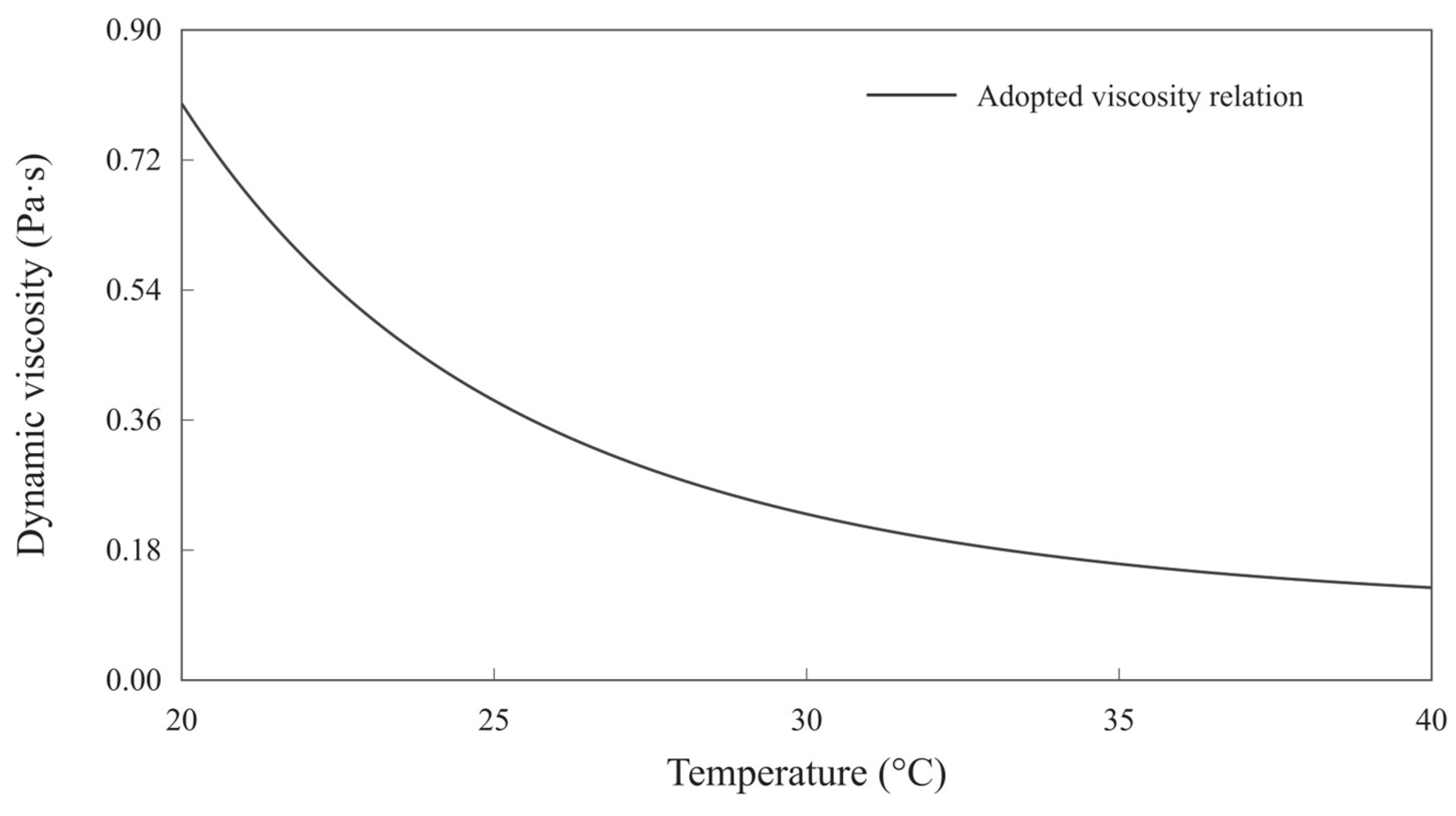
This temperature-only relation is used solely for this reproduction. It does not represent cooling or shear history, wax precipitation, or deposition.
The two-dimensional ground-surface heat transfer coefficient is 18.60 W/(m2·K). Ambient and bottom-boundary temperatures are both 0 °C; the far-side and symmetry boundaries are adiabatic. The 1D FVM and analytical resistance model use an equivalent soil cylinder of outer radius H, with the same external coefficient and ambient temperature. The analytical model includes an external convection resistance R’ext = 1/(2πHho), where R’ext is resistance per unit pipe length, m·K/W. The equivalent cylindrical boundary and the planar ground surface are geometrically different.
The independent two-dimensional right half-domain is 10 m wide and 10 m deep. Its 48/288/0.5 mesh contains 38,626 control volumes. The 1D FVM uses 200 radial cells per layer and geometrically graded soil cells.
The analytical model and both FVMs update the internal heat transfer coefficient using the local fluid temperature and circumferential mean inner-wall temperature, rather than the fixed 300 W/(m2·K) used in the main comparison. The axial step is 100 m. Frictional heating and thermal-expansion corrections are retained in this independent case.
The local heat transfer coefficient and mean inner-wall temperature are iterated until their relative changes are below 10−10. The heat-transfer response is sampled at 0.5 °C intervals and interpolated.
DirectK uses an overall coefficient determined at the inlet condition and held constant downstream. This calibration is independent of the main-text calibration.
Appendix A.2. Comparison of Results
Table A2.
Published and recalculated results.
Refining the 2D mesh to 96/576/0.25 and the 1D mesh to 400 cells per layer changed outlet temperatures by 0.0003 and approximately 0.0001 °C, respectively. Halving the axial step and temperature-sampling interval changed outlet temperatures by less than 0.0012 and 0.00005 °C, respectively. These changes are smaller than the published-case differences in Table A2.
Appendix B. Numerical Verification
This appendix checks mesh, time-step, computational-domain, ground-boundary and startup sensitivity. The study-specific screening values are 0.5% for heat-loss changes, 0.05 °C for monitored-temperature changes, 0.02 °C for circumferential-range changes, 1 m for front-position changes and 0.01 m for paired front-position-difference changes. The relative physical energy-balance residual must be below 10−6. Refinement differences are sensitivity indicators, not error bounds relative to an exact solution or engineering safety limits.
Using the finer setting as the reference, heat losses are compared by absolute relative difference; temperatures and front positions are compared by absolute difference. Monitored temperatures include the inner wall, material interfaces and the top and bottom of the outermost pipe surface. The circumferential range is the maximum minus minimum temperature on that surface. Differences are computed before rounding; a displayed 0.0000 does not denote an exactly zero difference.
Appendix B.1. Mesh Refinement
The 1D FVM uses 100, 200 and 400 radial cells per layer with geometrically graded soil cells. The 2D FVM jointly refines radial, circumferential and soil resolution (Table A3). Mesh triples denote radial cells per pipe layer, full-circle equivalent circumferential cells and soil size scale, respectively. The computed half-domain contains half the stated circumferential cell count; a smaller soil size scale indicates a finer soil mesh.
Table A3.
Steady benchmark mesh-refinement results.
Under the same temperature conditions as Table A3, joint refinement from 24/144/0.5 to 48/288/0.25 for the benchmark and geometries C and D changed heat loss and monitored temperatures by at most 0.0059% and 0.0061 °C, respectively. Circumferential-range changes were below 0.001 °C.
With the pipe-layer resolution fixed at 48/288, the soil size scale is reduced from 0.5 to 0.25. Transient results are compared at 2, 24, 168 and 720 h in Table A4. Initial and ambient temperatures are 20 °C and the fluid temperature is 80 °C.
Table A4.
Effect of soil-mesh refinement on transient results.
Increasing the 1D radial cell count per layer from 200 to 400 changed transient heat loss and monitored temperatures by at most 0.0046% and 0.0025 °C, respectively. The selected meshes therefore use 200 cells per layer in 1D and 48/288/0.5 in 2D.
Appendix B.2. Early-Time Time-Step Refinement
The benchmark transient starts at 10 °C, with ambient temperature 10 °C and fluid temperature raised to 80 °C. Results at 2 h are compared for time steps of 120, 60 and 30 s, using the 30 s solution as reference (Table A5).
Table A5.
Early-time time-step refinement.
Appendix B.3. Piecewise Time-Step Refinement
The benchmark transient is extended to 720 h. Sequences of 60/300/450 s and 30/150/225 s are compared over 0–2, 2–24 and 24–720 h, respectively (Table A6); the latter sequence is selected. The 720 h result is still treated as transient.
Table A6.
Piecewise radial time-step refinement.
Cases A–D use initial and ambient temperatures of 20 °C and fluid temperature 80 °C. Halving the time steps changed heat loss and monitored temperatures by less than 0.0026% and 0.0011 °C for A and B. Corresponding changes in the 2D results for C and D were below 0.0028% and 0.0013 °C.
Appendix B.4. Computational Domain and Ground Boundary
Keeping the pipe and near-field soil mesh fixed at 24/144/0.5, the domain is extended only sideways and downwards. Domains 6 and 8 times the unscaled dimensions in Section 2.4.1 are compared in Table A7 to distinguish boundary truncation from remeshing effects.
Table A7.
Domain extension with an unchanged near-field mesh.
The main results use domain scale 8: the benchmark right half-domain is 48 m wide and 60 m deep, and case C uses 320 m by 400 m. Steady changes from scales 6 to 8 satisfy the screening values. In the transient check with initial and ambient temperatures of 20 °C and fluid temperature 80 °C, the maximum monitored-temperature change at the checked times up to 720 h was below 0.000002 °C.
Replacing the 108 W/(m2·K) ground convection condition with an exact prescribed-temperature condition changed steady heat loss by less than 10−6% and monitored temperatures by less than 10−6 °C. Thus the large-coefficient approximation has negligible influence in the checked cases. The finite 18.60 W/(m2·K) boundary in Appendix A is a different physical condition, not a refinement of this approximation.
Appendix B.5. Startup Verification
To examine the effects of the axial grid and time step separately, 98,304, 196,608 and 393,216 axial control volumes were tested at a fixed time step of 0.2197265625 s. Time steps of 0.87890625, 0.439453125 and 0.2197265625 s were tested with 393,216 axial control volumes. The outlet-temperature histories over 0–24 h, axial temperature profiles at 2, 6, 12 and 24 h, and inter-model temperature differences were compared, as reported in Table A8.
With fixed properties and heat transfer coefficients, model reduction approximates the cross-sectional thermal response using a smaller system of equations, and a discrete Z-transform calculates the axial temperatures. The first-order upwind and backward-Euler discretizations remain unchanged. To check the accelerated calculation, the unreduced cross-sectional equations were solved directly by time marching under the same startup conditions and selected radial grids, using 24 axial control volumes with a time step of 1800 s and 48 control volumes with a time step of 900 s. These results were compared with accelerated calculations at matching settings. Over 0–24 h, discrepancies in both fluid temperatures and inter-model temperature differences were below 2.7 × 10⁻⁸ °C. This comparison checks consistency between the accelerated and direct solutions; it does not replace axial-grid and time-step refinement checks.
Table A8.
Separate axial-grid and time-step refinement of startup temperatures.
The thermal front is defined by the 45 °C position and compared from 2 h over the common interval in which the fronts remain inside the pipeline. The axial grid, time step and output-sampling parameters are varied separately, as reported in Table A9.
Table A9.
Separate refinement checks for startup front positions.
With the finest axial grid and time step fixed, doubling the inverse-transform sampling count changed the axial profiles by approximately 0.000245 °C at most and the front positions by less than 10−9 m. With 65,536 samples fixed, reducing the output spacing from 5 to 2.5 m changed the front positions and the inter-model front-position difference by at most 0.0052 and 0.0004 m, respectively. The final results use the finest axial grid and time step, 65,536 inverse-transform samples and a 2.5 m output spacing. These are numerical sensitivity checks, not rigorous error bounds or recommended routine engineering settings.
Appendix B.6. Known Solutions and Energy Balance
Implementation is checked against a prescribed two-dimensional linear temperature field, a steady composite-cylinder solution and a transient homogeneous-annulus Bessel-series solution (Table A10). The linear field uses conductivity 1.5 W/(m·K), temperature 2 °C at the origin, and horizontal and vertical gradients of 0.37 and −0.91 K/m. Boundary temperatures are imposed from that field.
The composite cylinder uses the main-text pipe structure and properties without soil. Fluid and external temperatures are 80 and 10 °C, and the internal coefficient is 300 W/(m2·K). Each layer has 48 radial cells and the full-circle equivalent circumferential cell count is 288.
The homogeneous annulus has inner and outer radii of 0.14 and 0.203 m, conductivity 50 W/(m·K) and volumetric heat capacity 3.5 × 10⁶ J/(m3·K). Initial and outer-boundary temperatures are 10 °C; the inner fluid temperature is 80 °C with coefficient 300 W/(m2·K). A 48/192 mesh and 0.5 s time step are used. Temperatures and inner-boundary heat losses are compared with the Bessel-series solution at 10, 60, 120, 300 and 600 s.
Table A10.
Comparison with analytical solutions and the prescribed temperature field.
Physical energy balance is checked using changes in stored energy and boundary heat flows, with residuals normalized by input and output heat rates. Maximum relative residuals were 5.3 × 10⁻⁹ for the A–D radial calculations up to 720 h and 7.2 × 10⁻⁸ for startup. These tests verify numerical implementation and do not replace experimental or field validation.
References
- Yu, B.; Li, C.; Zhang, Z.; Liu, X.; Zhang, J.; Wei, J.; Sun, S.; Huang, J. Numerical simulation of a buried hot crude oil pipeline under normal operation. Appl. Therm. Eng. 2010, 30, 2670–2679. [Google Scholar] [CrossRef] [Scilit]
- Xing, X.; Dou, D.; Li, Y.; Wu, C. Optimizing control parameters for crude pipeline preheating through numerical simulation. Appl. Therm. Eng. 2013, 51, 890–898. [Google Scholar] [CrossRef] [Scilit]
- Li, G.; Sheng, Y.; Jin, H.; Ma, W.; Qi, J.; Wen, Z.; Zhang, B.; Mu, Y.; Bi, G. Forecasting the oil temperatures along the proposed China–Russia Crude Oil Pipeline using quasi 3-D transient heat conduction model. Cold Reg. Sci. Technol. 2010, 64, 235–242. [Google Scholar] [CrossRef] [Scilit]
- Yuan, Q.; Luo, Y.; Shi, T.; Gao, Y.; Wei, J.; Yu, B.; Chen, Y. Investigation into the heat transfer models for the hot crude oil transportation in a long-buried pipeline. Energy Sci. Eng. 2023, 11, 2169–2184. [Google Scholar] [CrossRef] [Scilit]
- Dehdarinejad, M.; Behbahani-Nejad, M.; Hajidavalloo, E. Experimental and numerical investigation of heat loss in transition modes of buried hot fuel oil pipeline. Proc. Inst. Mech. Eng. Part C J. Mech. Eng. Sci. 2021, 235, 6567–6576. [Google Scholar] [CrossRef] [Scilit]
- Bossinov, D.; Ramazanova, G.; Turalina, D. Comparison of measured and calculated high-viscosity crude oil temperature values in a pipeline during continuous pumping and shutdown modes. Int. J. Thermofluids 2024, 24, 100950. [Google Scholar] [CrossRef] [Scilit]
- Zhou, G.; Xie, Z.-W.; Xu, X.-H.; Li, Q. A new model of overall heat transfer coefficient of hot wax oil pipeline based on dimensionless experimental analysis. Case Stud. Therm. Eng. 2020, 20, 100647. [Google Scholar] [CrossRef] [Scilit]
- Thiyagarajan, R.; Yovanovich, M.M. Thermal Resistance of a Buried Cylinder With Constant Flux Boundary Condition. J. Heat Transf. 1974, 96, 249–250. [Google Scholar] [CrossRef] [Scilit]
- Bau, H.H.; Sadhal, S.S. Heat losses from a fluid flowing in a buried pipe. Int. J. Heat Mass Transf. 1982, 25, 1621–1629. [Google Scholar] [CrossRef] [Scilit]
- Chung, M.; Jung, P.-S.; Rangel, R.H. Semi-analytical solution for heat transfer from a buried pipe with convection on the exposed surface. Int. J. Heat Mass Transf. 1999, 42, 3771–3786. [Google Scholar] [CrossRef] [Scilit]
- Otomi, O.K.; Onochie, U.P.; Obanor, A.I. Steady state analysis of heat transfer in a fully buried crude oil pipeline. Int. J. Heat Mass Transf. 2020, 146, 118893. [Google Scholar] [CrossRef] [Scilit]
- Archer, R.A.; O’Sullivan, M.J. Models for Heat Transfer from a Buried Pipe. SPE J. 1997, 2, 186–193. [Google Scholar] [CrossRef] [Scilit]
- Chaczykowski, M. Transient flow in natural gas pipeline—The effect of pipeline thermal model. Appl. Math. Model. 2010, 34, 1051–1067. [Google Scholar] [CrossRef] [Scilit]
- Wei, L.; Lei, Q.; Zhao, J.; Dong, H.; Yang, L. Numerical simulation for the heat transfer behavior of oil pipeline during the shutdown and restart process. Case Stud. Therm. Eng. 2018, 12, 470–483. [Google Scholar] [CrossRef] [Scilit]
- Wei, L.; Dong, H.; Zhao, J.; Zhao, W.; Liu, J. Transient thermal characteristics of the buried crude oil pipeline system during the reverse pipelining. J. Therm. Anal. Calorim. 2021, 145, 2503–2524. [Google Scholar] [CrossRef] [Scilit]
- Chen, Z.; Yuan, Q.; Jiang, W.; Li, Z.; Yu, B. Thermo-Hydraulic Characteristics of Non-Isothermal Batch Transportation Pipeline System with Different Inlet Oil Temperature. J. Therm. Sci. 2023, 32, 965–981. [Google Scholar] [CrossRef] [Scilit]
- Oosterkamp, A.; Ytrehus, T.; Galtung, S.T. Effect of the choice of boundary conditions on modelling ambient to soil heat transfer near a buried pipeline. Appl. Therm. Eng. 2016, 100, 367–377. [Google Scholar] [CrossRef] [Scilit]
- Xie, H.; Li, C.; Jia, W.; Zhang, C. Three-Dimensional CFD Modeling on the Thermal Characteristics of Buried Oil Pipeline Involving the Heat Transfer of Wax Layer. Energies 2022, 15, 6022. [Google Scholar] [CrossRef] [Scilit]
- Yuan, Q.; Jiang, W.; Guo, M.; Chen, Y.; Yu, B.; Wei, J. GPU-accelerated transient thermo-hydraulic simulation of weakly compressible restart flow of a non-Newtonian fluid in a long-buried hot oil pipeline. Appl. Therm. Eng. 2023, 227, 120299. [Google Scholar] [CrossRef] [Scilit]
- Xie, H.; Li, C.; Wei, N.; Zhang, C.; He, J. Numerical Study on the Optimal Thermally Affected Region of a Buried Oil Pipeline. ACS Omega 2023, 8, 27761–27775. [Google Scholar] [CrossRef] [Scilit] [PubMed]
- Jiang, M.; Speetjens, M.F.M.; Rindt, C.C.M.; Smeulders, D.M.J. A data-based reduced-order model for dynamic simulation and control of district-heating networks. Appl. Energy 2023, 340, 121038. [Google Scholar] [CrossRef] [Scilit]
- Meibodi, S.S.; Rees, S. Experimental validation of the dynamic thermal network approach in modeling buried pipes. Sci. Technol. Built Environ. 2023, 29, 589–605. [Google Scholar] [CrossRef] [Scilit]
- Yan, F.; Jiao, K.; Nie, C.; Han, D.; Li, Q.; Chen, Y. Fast Prediction of the Temperature Field Surrounding a Hot Oil Pipe Using the POD-BP Model. Processes 2023, 11, 2666. [Google Scholar] [CrossRef] [Scilit]
- Yu, G.; Yu, B.; Han, D.; Wang, L. Unsteady-state thermal calculation of buried oil pipeline using a proper orthogonal decomposition reduced-order model. Appl. Therm. Eng. 2013, 51, 177–189. [Google Scholar] [CrossRef] [Scilit]
- Jiang, W.; Wang, J.; Varbanov, P.S.; Yuan, Q.; Chen, Y.; Wang, B.; Yu, B. Hybrid data-mechanism-driven model of the unsteady soil temperature field for long-buried crude oil pipelines with non-isothermal batch transportation. Energy 2024, 292, 130354. [Google Scholar] [CrossRef] [Scilit]
- Li, Q.; Zhou, C.; Yan, F.; Xu, J.; Ji, M.; Gong, J.; Chen, Y.; Zhao, Y.; Han, D.; Wang, P. Fast prediction of coupled oil and environment temperature fields during shutdown of buried waxy crude oil pipelines using neural networks. Phys. Fluids 2025, 37, 013113. [Google Scholar] [CrossRef] [Scilit]
- Yan, F.; Xu, J.; Li, Q.; Zhou, C.; Ji, M.; Gong, J.; Xiang, Y.; Chen, Y.; Han, D.; Wang, P. Rapid Prediction Models for Oil Temperature and Surrounding Environment Temperature Fields in Buried Hot Crude Oil Pipelines. J. Pipeline Syst. Eng. Pract. 2025, 16, 04025043. [Google Scholar] [CrossRef] [Scilit]
- Wieland, A.; Dollhopf, S.; Weidlich, I.; Langroudi, P.P. Heat Loss Determination of District Heating Pipelines. A Comparison of Numerical and Analytical Methods. Environ. Clim. Technol. 2024, 28, 927–939. [Google Scholar] [CrossRef] [Scilit]
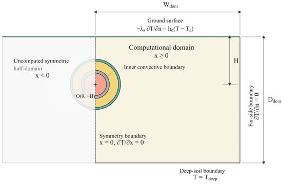
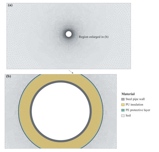
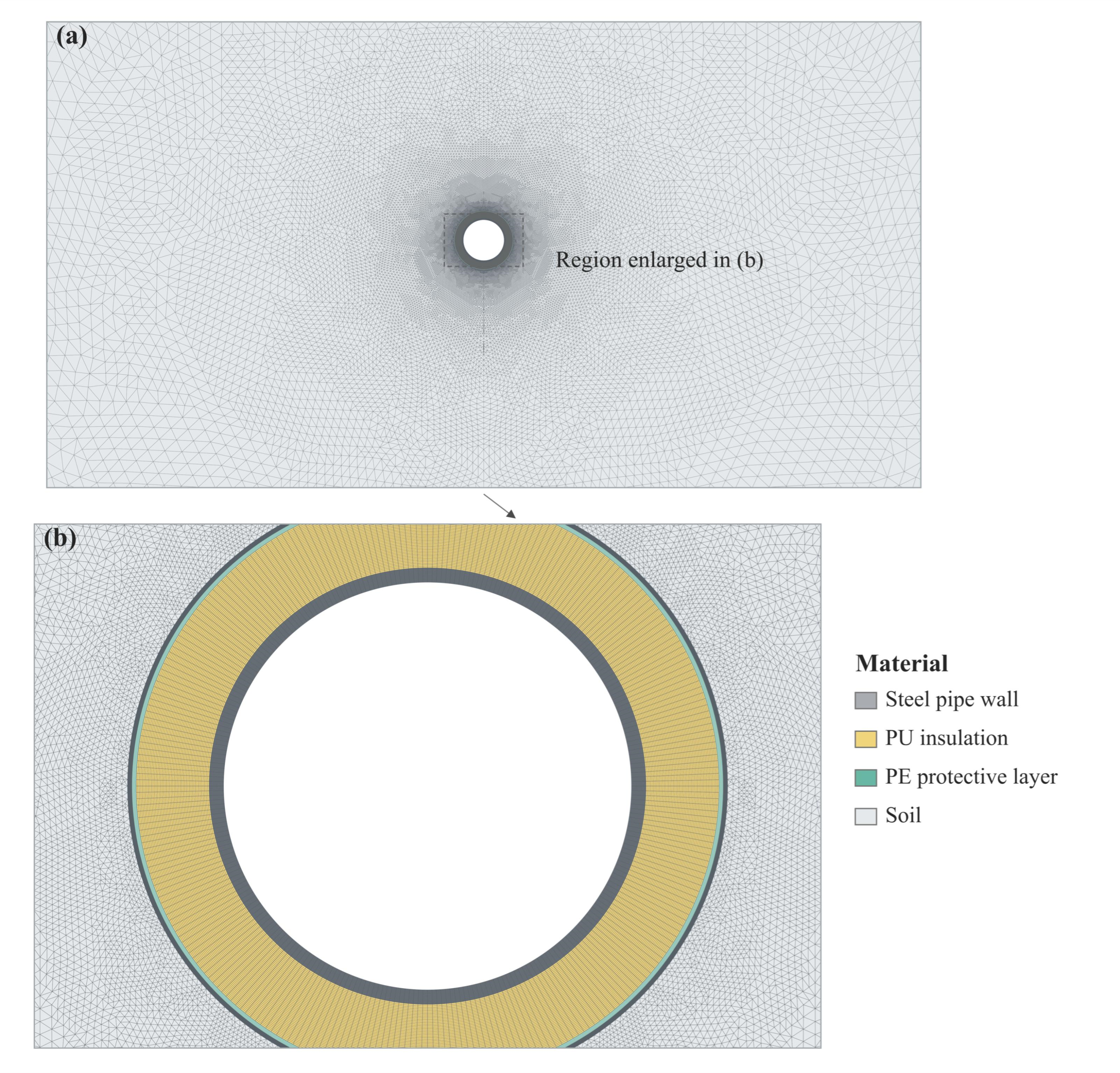
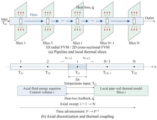
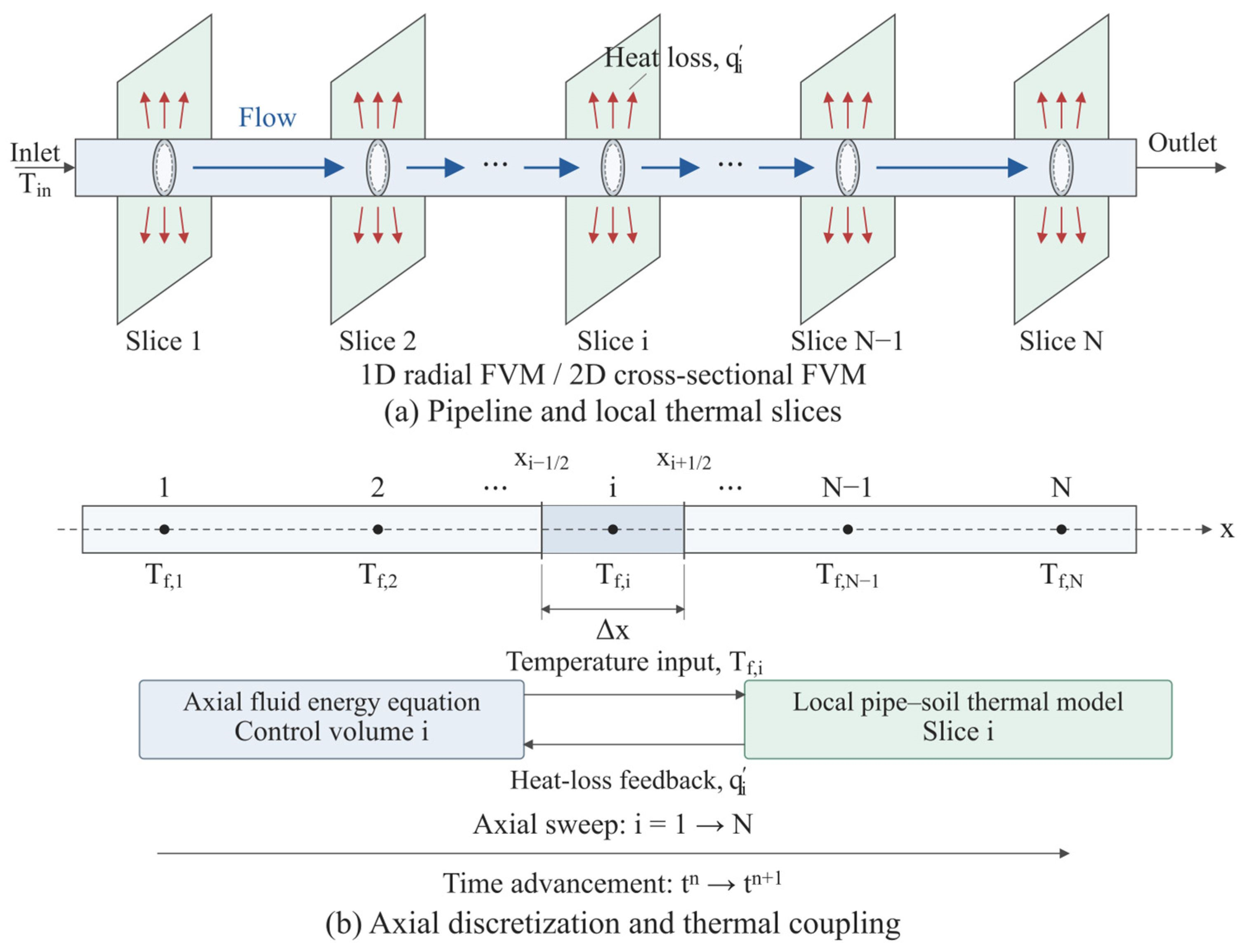
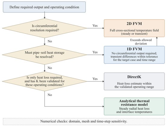
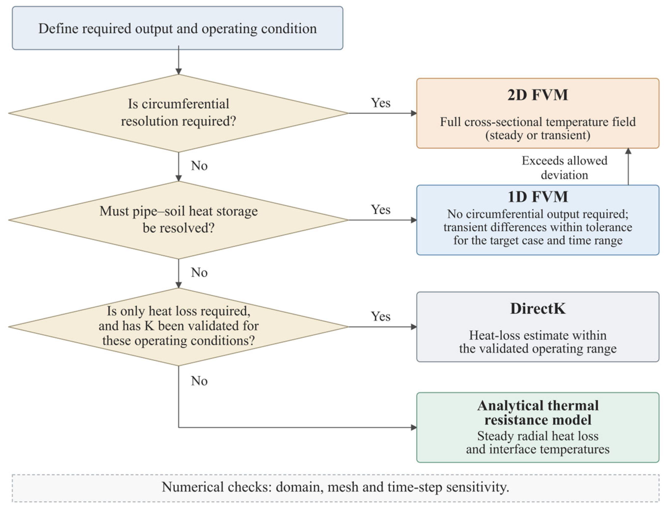
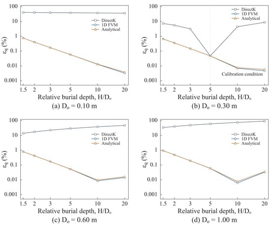
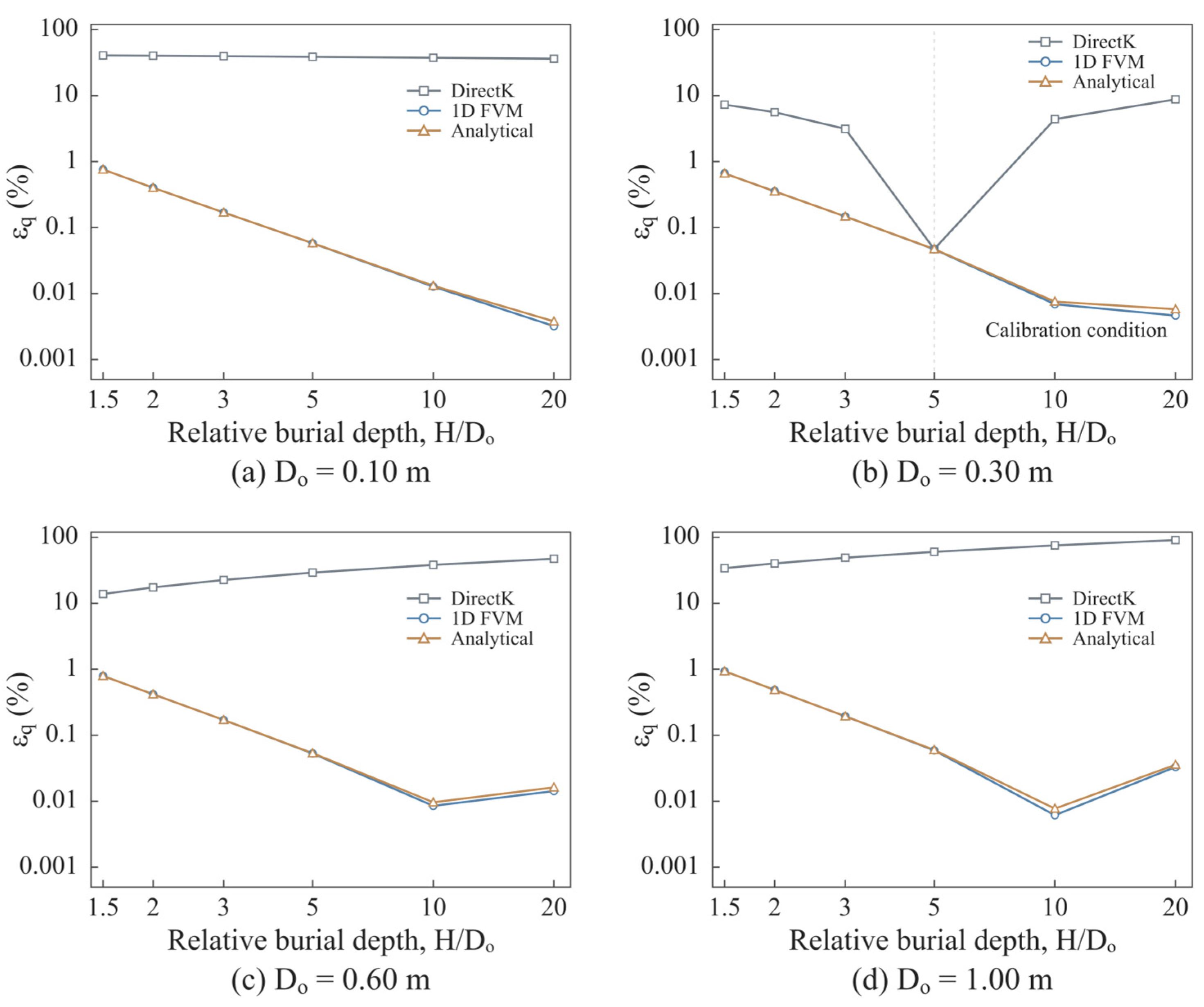
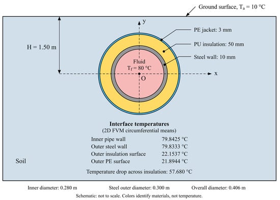
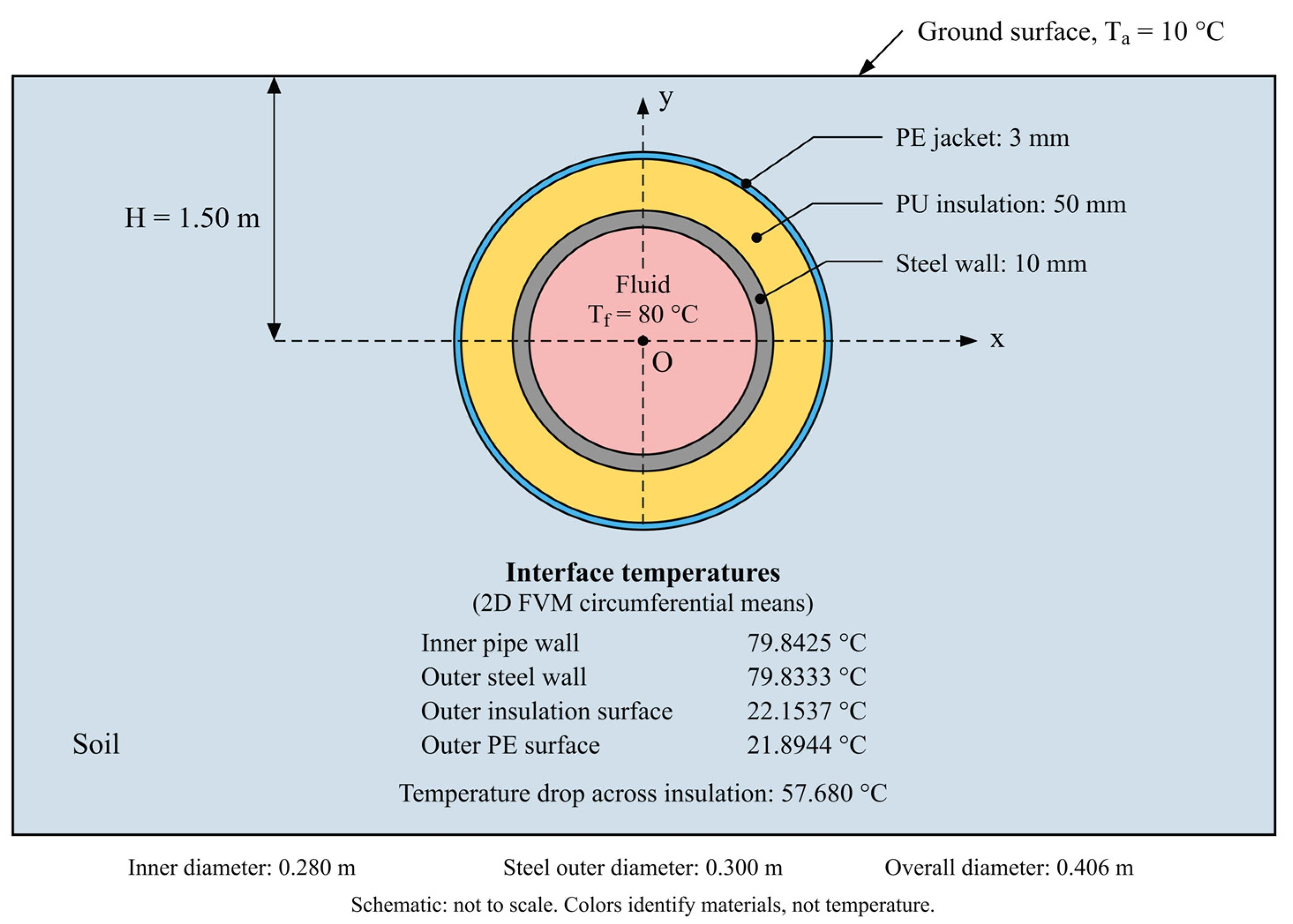
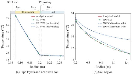
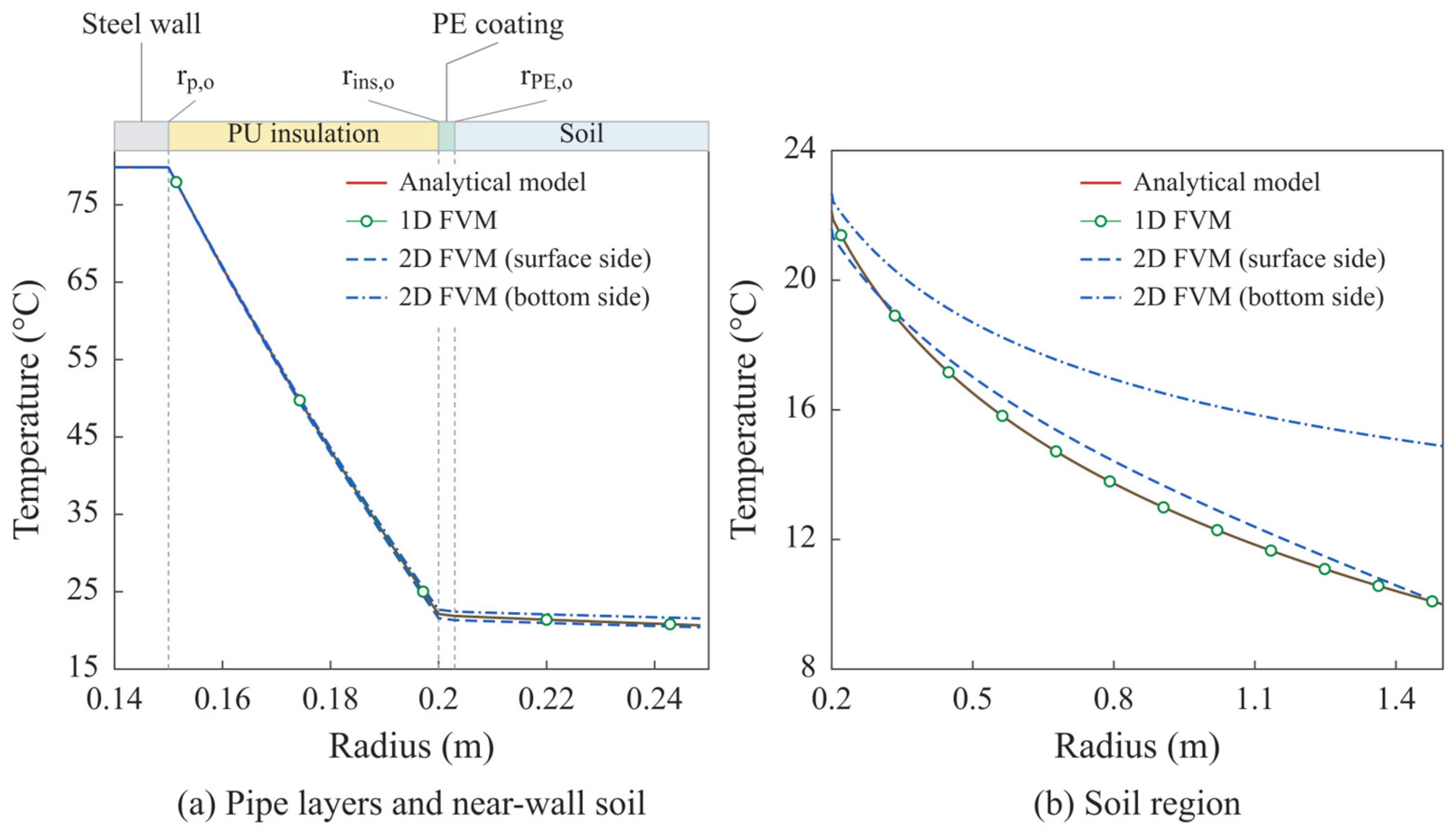
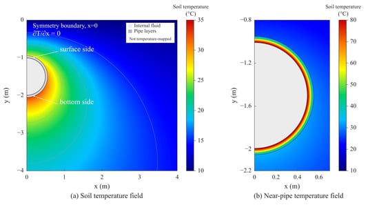
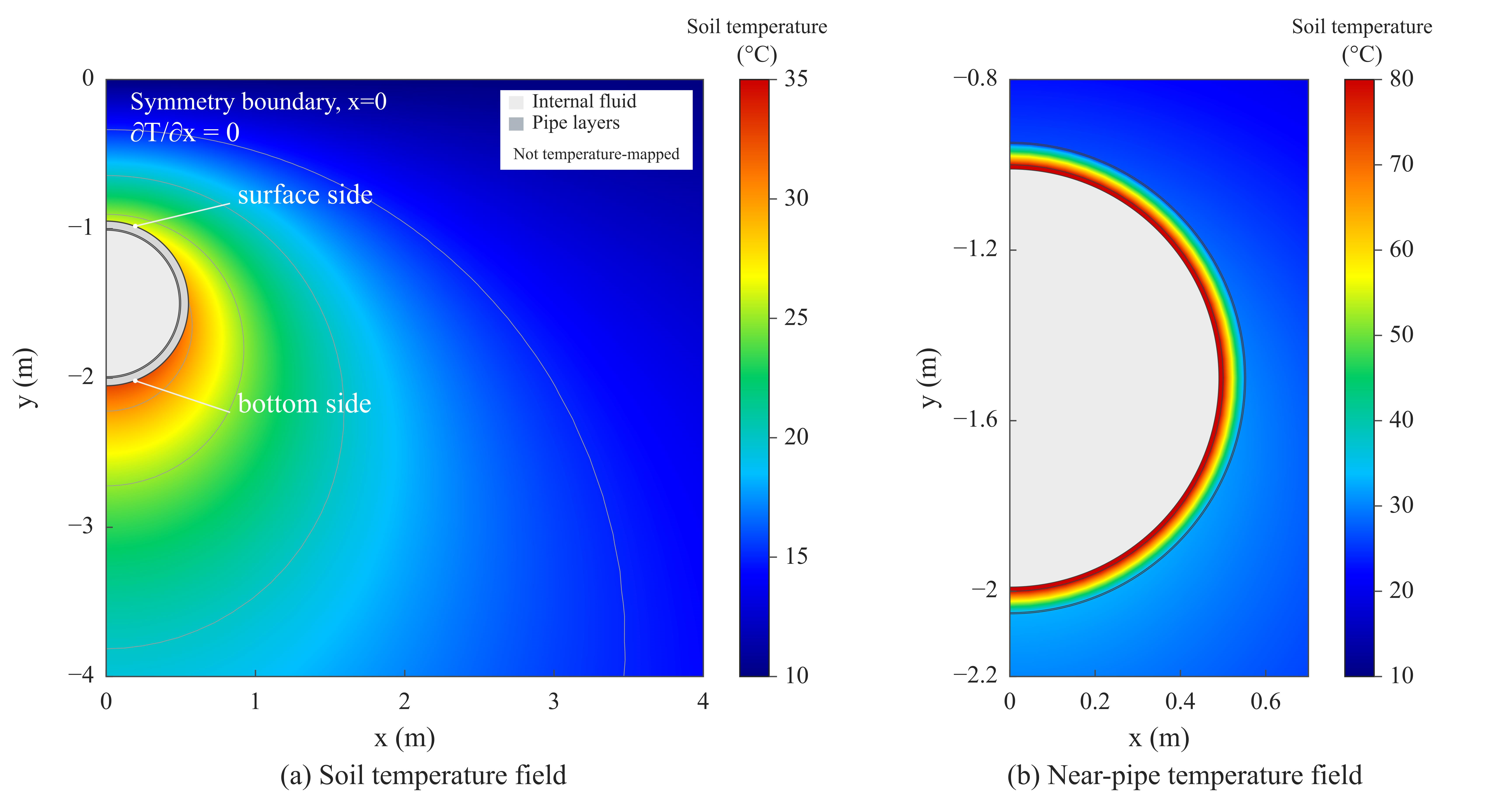
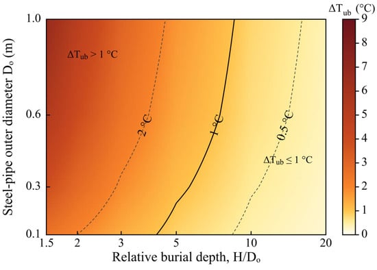
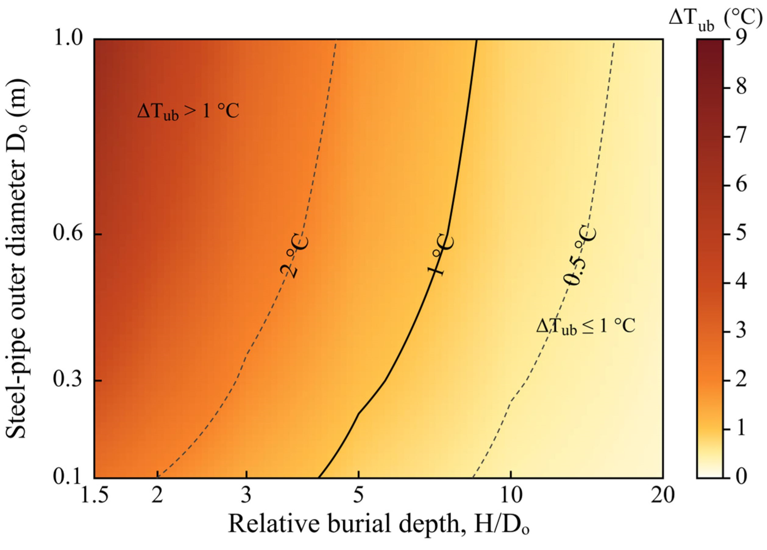
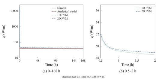
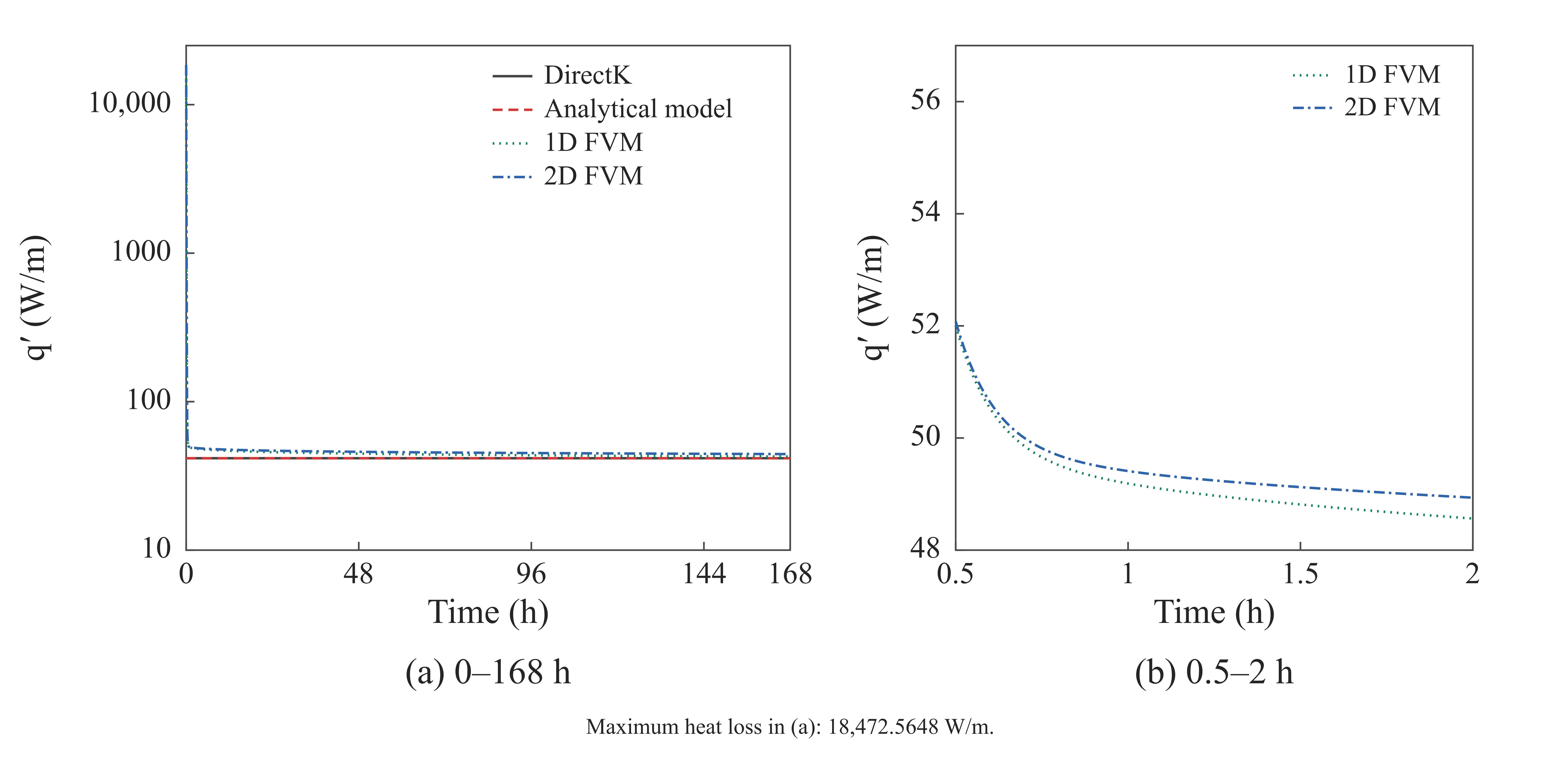
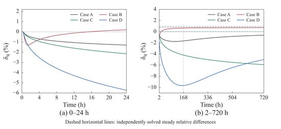
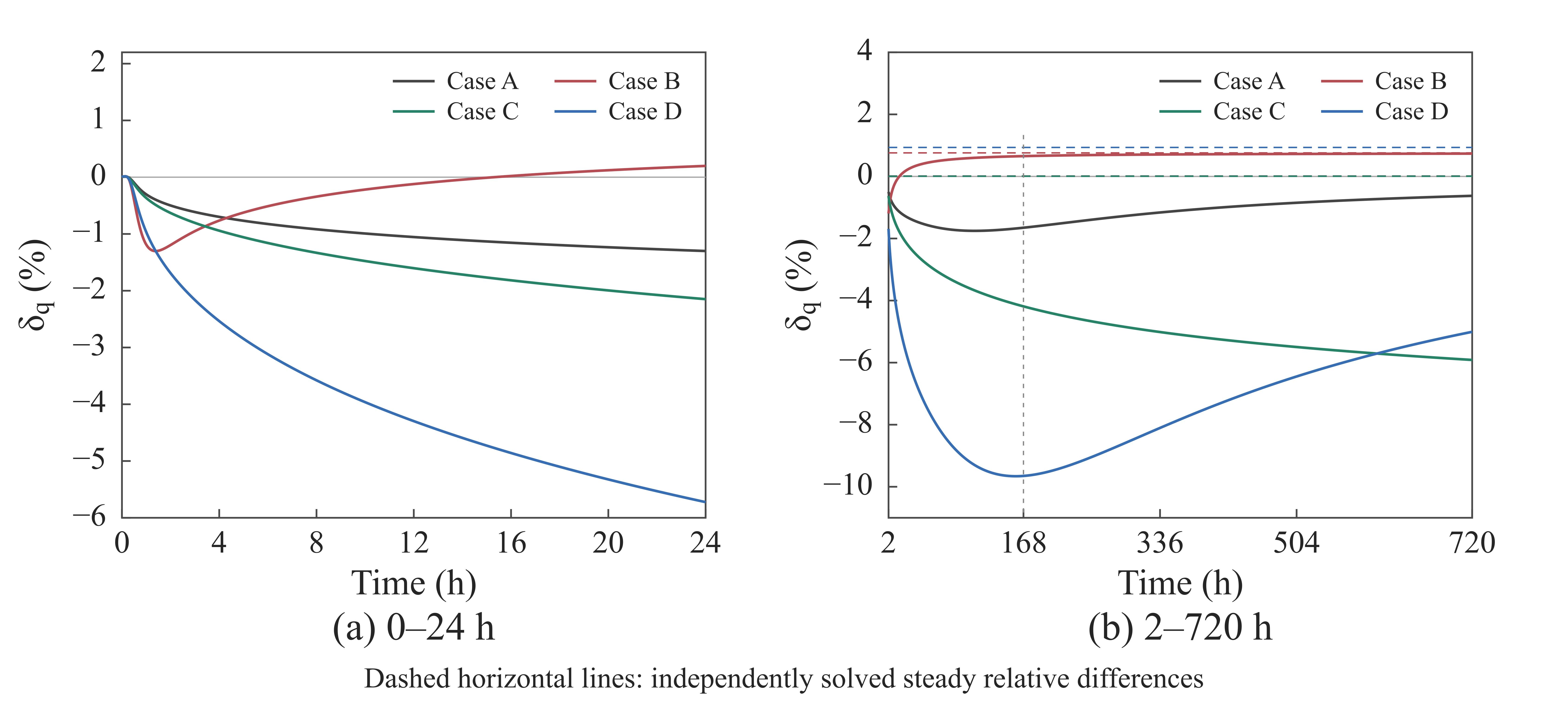
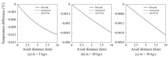
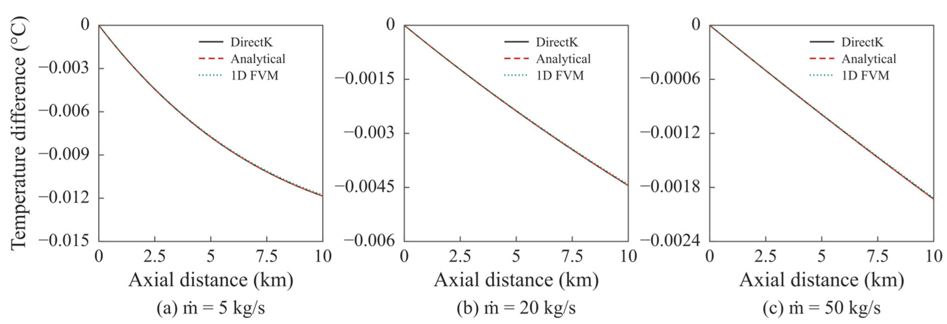
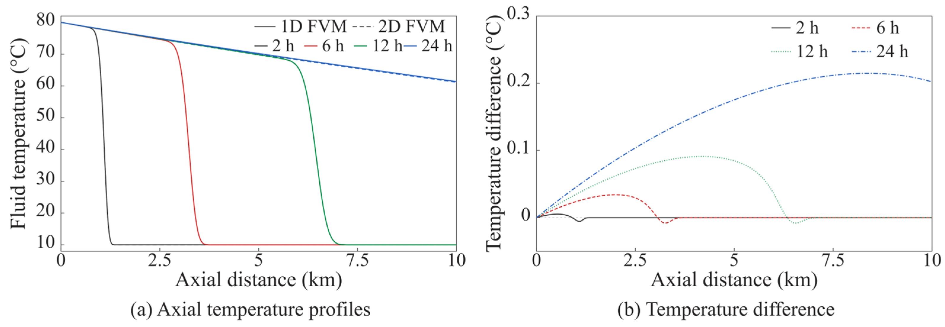

Disclaimer/Publisher’s Note: The statements, opinions and data contained in all publications are solely those of the individual author(s) and contributor(s) and not of MDPI and/or the editor(s). MDPI and/or the editor(s) disclaim responsibility for any injury to people or property resulting from any ideas, methods, instructions or products referred to in the content. |
© 2026 by the authors. Licensee MDPI, Basel, Switzerland. This article is an open access article distributed under the terms and conditions of the Creative Commons Attribution (CC BY) license.