Virtual-Node-Enhanced Mirror-Equivalent Energy Framework for Online Transient Stability Assessment of EHV Transmission Lines

Abstract

Online transient stability assessment (TSA) is essential for the secure operation of long-distance extra-high-voltage (EHV) transmission lines. Mirror-equivalent energy (MEE) methods depend on accurate center-of-oscillation (CoO) localization, but conventional two-terminal frequency interpolation may inadequately represent internal frequency variations in long EHV lines. Measurement noise can further affect weighted least-squares (WLS) state estimates and subsequent energy assessment. This paper proposes a virtual-node-enhanced MEE framework that reconstructs internal frequency responses using extended Kalman filter (EKF)-estimated generator states and a multi-section π-equivalent transmission-line model. The CoO is located through linear-regression analysis and used to construct the mirror-equivalent system and calculate the MEE index. The framework is evaluated using a PSS/E model of a 750 kV, 300 km double-circuit transmission line in the Northwest China Power Grid. In the representative stable and unstable cases of the studied system, virtual-node reconstruction reduces the absolute CoO location errors from 5.236 to 3.281 km and from 65.021 to 0.349 km, respectively, compared with two-terminal interpolation. In 200 paired Monte Carlo trials at SNRs of 40 and 30 dB, the EKF-based method produces smaller mean CoO location errors and no incorrect stability decisions, whereas the WLS-based method produces seven incorrect decisions. Additional simulations evaluate the framework under different pre-fault transfer powers, fault locations, fault types, and clearing times. These results demonstrate improved CoO localization accuracy and more reliable stability assessment under the tested conditions.

1. Introduction

Extra-high-voltage (EHV) transmission systems are widely used for long-distance bulk-power transfer because they provide high transfer capability with comparatively low transmission losses [1]. The 750 kV AC network forms the backbone of the Northwest China Power Grid and supports substantial inter-area power transfer [2]. Severe faults on heavily loaded EHV transmission lines can produce large inter-area power imbalances, resulting in pronounced rotor-angle swings and possible loss of synchronism [1,3]. Timely and reliable online transient stability assessment (TSA) is therefore required to determine whether interconnected generators will remain in synchronism following such disturbances.

Existing transient stability assessment methods can be broadly categorized into three groups: time-domain simulation-based methods, data-driven methods, and energy-function-based methods. Time-domain simulation provides detailed post-fault responses and remains a standard approach for offline stability analysis; however, its computational burden may limit its application to rapid online screening [4,5]. Data-driven methods can identify the stability state rapidly after training, but their performance depends on the coverage of operating conditions and disturbances in the training data [6,7,8,9,10,11]. Recent developments include adaptive PMU-cluster-based assessment under data loss and measurement noise [12] and the integration of Lyapunov stability theory into neural networks to improve physical interpretability [11]. Energy-function-based methods provide a physically interpretable alternative by comparing the post-fault system energy with a stability-energy boundary [13,14,15,16,17]. These methods reduce the need for extended post-fault simulation and are therefore suitable for rapid online assessment.

Among energy-function-based approaches, the mirror-equivalent energy (MEE) method supports online TSA by constructing a compact two-machine equivalent system through reflection of the generator of interest and the retained network about the center of oscillation (CoO) [18,19]. The resulting energy index is calculated from the relative rotor angle and speed of the original and mirror generators and is compared with a stability-energy threshold to assess post-fault synchronism. The MEE method therefore provides a computationally efficient and physically interpretable means of post-fault stability identification. However, its reliability depends strongly on the accuracy of the estimated generator states and the CoO location. Here, CoO localization refers to determining the position of the CoO along the monitored transmission line.

The conventional MEE method [19] locates the CoO by finding the distance-weighted combination of line-end frequencies with the smallest fitting error. For long EHV lines, the effects of distributed line parameters may limit the accuracy of approximating the internal frequency distribution by a distance-weighted combination of the two terminal frequencies [20,21]. In addition, measurement noise can introduce errors into WLS-based state estimates and consequently affect CoO localization and energy assessment [22,23,24,25]. The main research gap addressed in this study is the limited representation of internal frequency variations in conventional MEE-based CoO localization for long EHV transmission lines.

To address these limitations, this paper proposes a virtual-node-enhanced MEE framework. The main objective is to improve CoO localization accuracy and the reliability of online TSA for long EHV transmission lines. The monitored transmission line is represented by a multi-section π-equivalent model, whose internal computational nodes are termed virtual nodes. Virtual-node reconstruction refers to calculating the internal frequency responses, namely the time-varying frequencies at these nodes, from the EKF-estimated generator states and line parameters. The virtual-node reconstruction improves the spatial frequency representation used for CoO localization, while the EKF mitigates noise-induced state-estimation errors. The estimated CoO is subsequently used to construct the mirror-equivalent system and calculate the MEE index for post-fault stability assessment. The proposed framework is evaluated using a PSS/E model of a 750 kV, 300 km double-circuit transmission line representing the studied system in the Northwest China Power Grid. The main contributions are summarized as follows:

-

A virtual-node-based CoO localization procedure incorporates line parameters into internal frequency reconstruction, replacing the conventional single end-to-end interpolation with a section-by-section frequency representation.

-

An integrated framework combines EKF state estimation, virtual-node reconstruction, and MEE assessment to improve CoO localization and reduce the effects of noisy PMU measurements on stability decisions.

-

Comparative simulations with conventional two-terminal interpolation and WLS-based state estimation demonstrate the improvements in CoO localization accuracy and noise robustness provided by virtual-node reconstruction and EKF, respectively.

2. Materials and Methods

This section presents the proposed virtual-node-enhanced MEE framework for online TSA of long EHV transmission lines. First, the dynamic and measurement models of the monitored system are formulated, and an EKF is applied to estimate the system dynamic states from phasor measurement unit (PMU) measurements. Second, the estimated states are combined with the transmission-line parameters to calculate the frequency responses at internal virtual nodes of the multi-section π-equivalent line model. Third, the CoO is located by evaluating candidate locations within each interval between adjacent virtual nodes and identifying the location with the minimum linear-regression fitting error. Finally, the estimated CoO is used to construct the mirror-equivalent system, calculate the MEE index, and identify the post-fault response as stable or unstable. Figure 1 summarizes the main steps of the proposed framework, which are described in the following subsections.

Figure 1. Main steps of the proposed framework.

2.1. System Description and Modeling

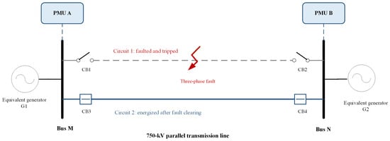
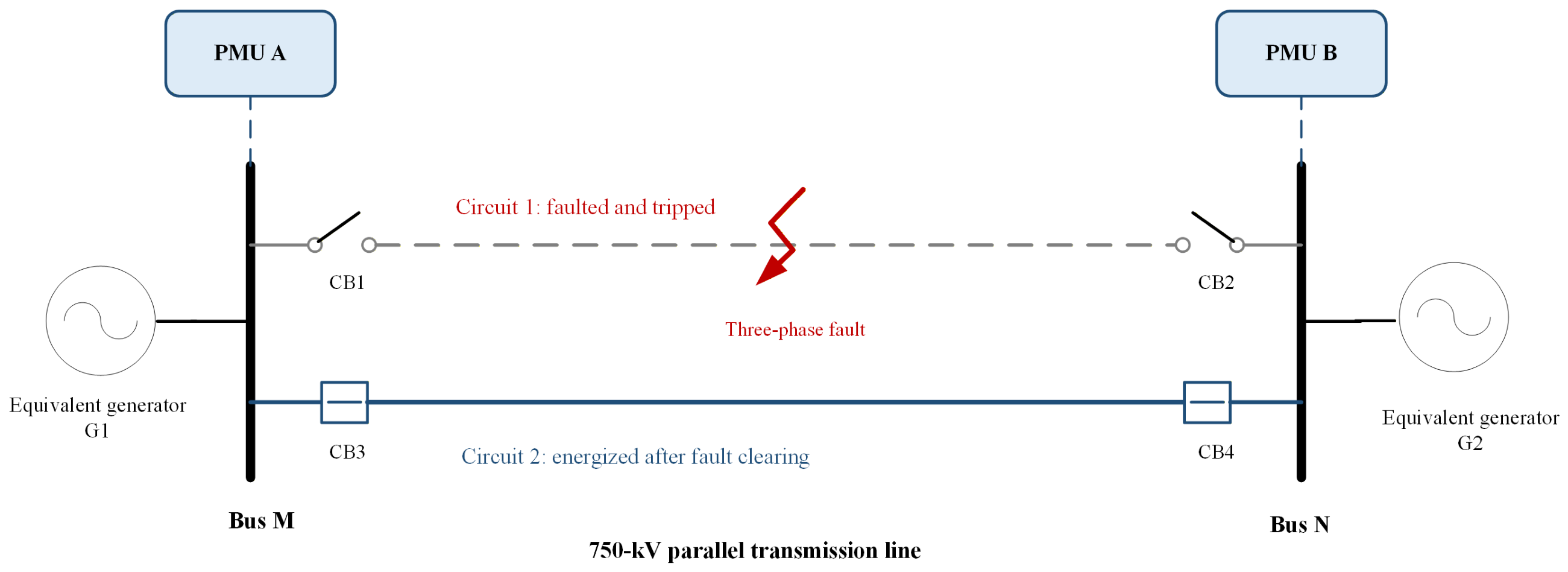
As shown in Figure 2, the sending- and receiving-end power systems are represented by machines G1 and G2, respectively, and are interconnected by a 750 kV, 300 km double- circuit transmission line. The two machines are characterized by their respective dynamic and electrical parameters. PMUs installed at buses M and N provide synchronized measurements of voltage phasors, line-current phasors, and bus frequencies. Following a fault on Circuit 1, the faulted circuit is tripped, while Circuit 2 remains energized and provides the electrical connection required for post-fault assessment.

Figure 2. Monitored 750 kV two-machine equivalent system.

(1)

Two-machine dynamic model: Let δ_i and Δω_i denote the electrical rotor angle and per-unit speed deviation of equivalent generator i, respectively. The rotor-angle and speed dynamics are described by

$$\begin{array}{c}\dot{{\Delta }_i}={\omega }_s{\Delta \mathsf{\omega }}_i\\ \hspace{1em}\hspace{1em}\hspace{1em}\hspace{1em}\hspace{1em}\hspace{1em}\hspace{1em}\hspace{1em}\hspace{1em}\hspace{1em}\hspace{1em}\hspace{1em}\hspace{1em}\hspace{1em}\hspace{1em}\hspace{1em}\hspace{1em}\hspace{1em}\hspace{1em}\hspace{1em}\hspace{1em}\hspace{1em}\hspace{1em}i\in \left\{1,2\right\}\\ \dot{{\Delta \mathsf{\omega }}_i}={\displaystyle \frac{P_{\mathit{mi}}-P_{\mathit{ei}}-D_i{\Delta \mathsf{\omega }}_i}{2H_i}}\end{array}$$

(1)

Here, H_i and D_i denote the equivalent inertia constant and damping coefficient, respectively; P_mi is the mechanical power input, and P_ei is the electrical power output. The per-unit speed deviation is defined as ${\Delta \mathsf{\omega }}_i={\displaystyle \frac{{\omega }_i-{\omega }_s}{{\omega }_s}}$, where ω_s is the synchronous angular speed.

(2)

Transmission line model: The EHV long transmission line is modeled by multiple equal π sections. This numerical representation captures the accumulated series impedance, shunt charging, and terminal shunt compensation of the long line. For each individual π section, the parameters are

z_ℓ = (r + jx)ΔL

y_ℓ = jω_scΔL

(2)

where r, x, and c are the series resistance, series reactance, and shunt capacitance per unit length; and ΔL denotes the length of each individual π section.

2.2. EKF-Based Dynamic State Estimation

Let x_k denote the dynamic state vector at sampling instant k:

$${\mathit{x}}_k={\left[{\Delta }_{1,k},{\Delta \mathsf{\omega }}_{1,k},{\Delta }_{2,k},{\Delta \mathsf{\omega }}_{2,k}\right]}^T$$

(3)

The nonlinear state-transition and PMU measurement models are expressed as

$$\begin{array}{c}{\mathit{x}}_k=\mathsf{\Phi }\left({\mathit{x}}_{k-1}\right)+{\mathit{w}}_{k-1},\\ {\mathit{z}}_k=\mathit{h}\left({\mathit{x}}_k\right)+{\mathit{v}}_k.\end{array}$$

(4)

where Φ (·) is obtained by discretizing the two-machine dynamic model over one PMU sampling interval and h(·) maps the state vector to the selected PMU measurements. The process and measurement noises are modeled as

w_k−1∼N(0,Q_k−1),v_k∼N(0,R_k)

(5)

where w_k−1 and v_k are the zero-mean process and measurement noise vectors, respectively, and Q_k−1 and R_k are their covariance matrices. The measurement vector contains the rectangular components of the voltage phasors at buses M and N, the current phasors measured at both ends of the remaining in-service circuit, and the two terminal frequencies.

Given the corrected state estimate ${\widehat{x^{+}}}_{k-1}$ and covariance P⁺_k−1, the EKF prediction step is

$$\begin{array}{c}{{\widehat{\mathit{x}}}_k}^{-}=\mathsf{\Phi }\left({{\widehat{\mathit{x}}}_{k-1}}^{+}\right)\\ {{\mathbf{P}}_k}^{-}={\mathbf{F}}_{k-1}{{\mathbf{P}}_{k-1}}^{+}{{\mathbf{F}}_{k-1}}^T+{\mathbf{Q}}_{k-1}\end{array}$$

(6)

where ${\mathbf{F}}_{k-1}={\displaystyle \frac{\partial \mathsf{\Phi }\left(\mathit{x}\right)}{\partial \mathit{x}}}{|}_{\mathit{x}={{\widehat{\mathit{x}}}_{k-1}}^{+}}$ is the state-transition Jacobian, and ${\mathbf{H}}_k={\displaystyle \frac{\partial \mathit{h}\left(\mathit{x}\right)}{\partial \mathit{x}}}{|}_{\mathit{x}={{\widehat{\mathit{x}}}_k}^{-}}$ is the measurement Jacobian.

The EKF measurement-update equations are:

$${\mathbf{S}}_k={\mathbf{H}}_k{{\mathbf{P}}_k}^{-}{{\mathbf{H}}_k}^T+{\mathbf{R}}_k$$

$$\begin{array}{c}{\mathbf{K}}_k={{\mathbf{P}}_k}^{-}{{\mathbf{H}}_k}^T{{\mathbf{S}}_k}^{-1}\\ {{\widehat{\mathit{x}}}_k}^{+}={{\widehat{\mathit{x}}}_k}^{-}+{\mathbf{K}}_k\left[{\mathit{z}}_k-\mathit{h}\left({{\widehat{\mathit{x}}}_k}^{-}\right)\right]\end{array}$$

(7)

$${{\mathbf{P}}_k}^{+}=\left(\mathbf{I}-{\mathbf{K}}_k{\mathbf{H}}_k\right){{\mathbf{P}}_k}^{-}$$

where S_k denotes the innovation covariance, K_k denotes the Kalman gain, ${{\widehat{\mathit{x}}}_k}^{+}$ denotes the corrected state estimate and ${{\mathbf{P}}_k}^{+}$ is the updated covariance matrix.

The EKF is initialized from the pre-fault PMU measurements. The initial rotor angles are obtained from the internal-voltage phasors calculated using the terminal voltages, currents, and equivalent reactance. The initial speed deviations are calculated from the terminal frequency deviations relative to the nominal frequency. The process noise covariance is set to Q = diag(10⁻⁸,10⁻⁹,10⁻⁸,10⁻⁹). For the noiseless simulations, R is diagonal, with entries of 10⁻⁸ p.u.² for the voltage and current rectangular components and 10⁻⁴ Hz² for the terminal frequencies. Nonzero entries are used to avoid singularity in the measurement update and allow for differences between the simulated measurements and the measurement model. State propagation uses a fourth-order Runge–Kutta method with a 1 ms internal integration step. The estimated rotor angles and speed deviations are subsequently used for the virtual-node frequency reconstruction presented in Section 2.3.

2.3. Virtual-Node-Based CoO Localization

The proposed procedure is initiated after the faulted circuit has been isolated and the breaker status confirms that the unfaulted circuit remains in service. It first reconstructs the frequencies at the internal virtual nodes using the EKF-estimated generator states and the transmission-line network equations and then locates the CoO through linear-regression analysis. By incorporating the line parameters into a section-by-section frequency reconstruction, the proposed method avoids the single end-to-end interpolation used in the conventional MEE formulation and improves CoO localization for long EHV lines.

(1)

Virtual-Node Frequency Reconstruction

To reconstruct the internal frequency distribution of the long line, the internal junctions between adjacent π sections of the transmission-line model established in Section 2.1 are designated as virtual nodes. The EKF processes the terminal voltage, current, and frequency measurements to estimate the generator rotor angles and speed deviations. These estimates, together with the line parameters, are used to calculate the virtual-node voltage phasors and frequencies through the post-fault network equations. These intermediate frequency values incorporate the effects of the line parameters, thereby enabling a more accurate section-by-section reconstruction of the frequency distribution along the entire line than the conventional single end-to-end interpolation based only on the two line-end frequencies.

Using the rotor-angle and speed-deviation estimates obtained in Section 2.2, the estimated internal-voltage phasor of generator i and its time derivative are expressed as:

$$\begin{array}{c}\widehat{E_{i,k}}={E_i}^{\prime }{e}^{j\widehat{{\Delta }_{i,k}}}\\ \dot{\widehat{E_{i,k}}}=j{\omega }_s{\Delta \widehat{\omega }}_{i,k}\widehat{E_{i,k}},i\in \left\{1,2\right\}\end{array}$$

(8)

where E′_i is the constant transient internal voltage.

Let ${\widehat{\mathit{E}}}_k=[{\widehat{E}}_{1,k},{\widehat{E}}_{2,k}{]}^T$, and let ${\widehat{\mathit{V}}}_k$ collect the voltage phasors at buses M and N and all internal virtual nodes of the remaining in-service circuit. Applying nodal analysis to the post-fault network yields:

$$\mathit{Y}{\widehat{\mathit{V}}}_k=\mathit{B}{\widehat{\mathit{E}}}_k,$$

(9)

where Y is the nodal-admittance matrix of the post-fault network, and B is the source-connection matrix relating the two generator internal voltages to buses M and N. Solving (9) for ${\widehat{\mathit{V}}}_k$ gives

$${\widehat{\mathit{V}}}_k=\mathit{G}{\widehat{\mathit{E}}}_k,\mathit{G}={\mathit{Y}}^{-1}\mathit{B},$$

(10)

where G is the voltage-transfer matrix. Because the post-fault network remains unchanged over the assessment window, G is constant. Differentiating (10) therefore gives

$${\dot{\widehat{\mathbf{V}}}}_k=G{\dot{\widehat{\mathbf{E}}}}_k$$

(11)

For any node n included in ${\widehat{\mathit{V}}}_k$, let ${\widehat{\mathit{V}}}_{n,k}=\left|{\widehat{\mathit{V}}}_{n,k}\right|e^{j{\widehat{\theta }}_{n,k}}$. Its voltage phase-angle derivative and frequency are given by

$$\begin{array}{c}{\dot{\widehat{\theta }}}_{n,k}={\displaystyle \frac{\mathrm{Im}\left\{{\widehat{V}}_{n,k}^{*}{\dot{\widehat{V}}}_{n,k}\right\}}{{\left|{\widehat{V}}_{n,k}\right|}^2}},\\ {\widehat{f}}_{n,k}=f_0+{\displaystyle \frac{{\dot{\widehat{\theta }}}_{n,k}}{2\pi }},\end{array}$$

(12)

where f₀ is the nominal system frequency. Using (12), the frequencies at the two line-end buses and all internal virtual nodes are calculated.

(2)

CoO Localization Using Reconstructed Frequencies

After obtaining the reconstructed nodal frequencies, the CoO is located by evaluating candidate positions within each adjacent-node interval and selecting the position that yields the global minimum regression fitting error over the entire monitored line. Unlike the conventional line-end-based formulation, the proposed method calculates the frequency at each candidate position from the two adjacent reconstructed nodal frequencies rather than from a single interpolation between the two line ends.

Consider the line section bounded by adjacent nodes n and n + 1, wheren = 1,…,N_s and N_s is the total number of line sections. For a candidate position x within this section,

x = x_n + λΔL, 0 ≤ λ ≤ 1

(13)

$${\widehat{f}}_{n,\lambda }\left(t_i\right)=(1-\lambda ){\widehat{f}}_n\left(t_i\right)+\lambda {\widehat{f}}_{n+1}\left(t_i\right).$$

where x_n = (n − 1)ΔL is the distance of node n from bus M and λ denotes the normalized position within the section. ${\widehat{f}}_n\left(t_i\right)$ and ${\widehat{f}}_{n+1}\left(t_i\right)$ are the reconstructed frequencies at the two bounding nodes, and ${\widehat{f}}_{n,\lambda }\left(t_i\right)$ is the interpolated frequency at the candidate position.

Let $\{t_i{\}}_{i=1}^{N_w}$ denote the synchronized sampling instants within the observation window, where N_w is the number of samples. Following the CoO definition adopted in [19], its frequency is assumed to vary approximately linearly with time over a short post-fault window. At each candidate position, the reconstructed frequency samples are fitted using a first-order linear regression model. The regression coefficients are determined by

$$\left({\widehat{a}}_{n,\lambda },{\widehat{b}}_{n,\lambda }\right)=\mathit{arg}\underset{a,b}{\mathit{min}}{\displaystyle {\sum }_{i=1}^{N_w}}{\left[{\widehat{f}}_{n,\lambda }\left(t_i\right)-(a{t}_i+b)\right]}^2$$

(14)

The corresponding regression root mean square error (RMSE) is

$${\epsilon }_n\left(\lambda \right)=\sqrt{{\displaystyle \frac{1}{N_w}}{\displaystyle {\sum }_{i=1}^{N_w}}{\left[{\widehat{f}}_{n,\lambda }\left(t_i\right)-\left({\widehat{a}}_{n,\lambda }{t}_i+{\widehat{b}}_{n,\lambda }\right)\right]}^2}$$

(15)

The interval containing the CoO and its normalized position within that interval are jointly determined from

$$\left({\widehat{n}}_c,{\widehat{\lambda }}_c\right)=\underset{\begin{array}{l}n=1,\dots ,N_s\\ 0\le \lambda \le 1\end{array}}{{\displaystyle \mathit{argmin}{\epsilon }_n(\lambda )}}$$

(16)

The estimated CoO distance from bus M and its normalized position are then calculated as

$${\widehat{x}}_c=x_{{\widehat{n}}_c}+{\widehat{\lambda }}_c\Delta L,\hspace{1em}{\widehat{s}}_c={\displaystyle \frac{{\widehat{x}}_c}{L}},$$

(17)

where L = N_sΔL is the total line length. Although candidate positions are evaluated within individual adjacent-node intervals, only the global minimum in (16) is retained. Therefore, the candidate location with the lowest regression RMSE is selected as the estimated CoO for the monitored line. The frequency at the identified CoO location ${\widehat{f}}_{c,k}={\widehat{f}}_{{\widehat{n}}_c,{\widehat{\lambda }}_c}\left(t_k\right)$ will be used in Section 2.4 for MEE-based stability assessment.

2.4. Mirror-Equivalent Energy-Based Stability Assessment

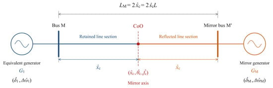
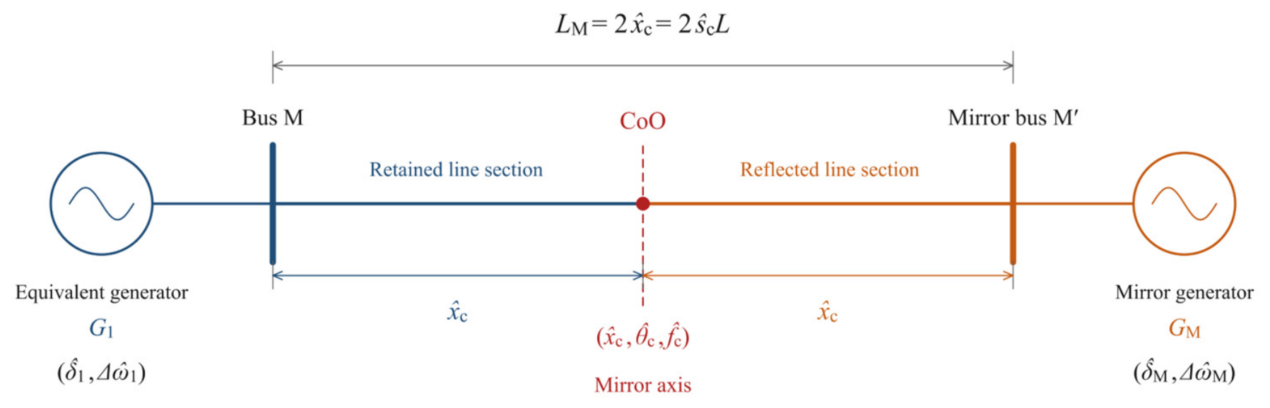
Using the CoO identified in Section 2.3, the subsystem consisting of equivalent generator G₁ and the retained line section between bus M and the CoO is reflected about the CoO to construct the mirror-equivalent system shown in Figure 3.

Figure 3. CoO-based mirror-equivalent system.

The relative rotor angle and angular speed of the mirror-equivalent system are defined as:

$$\begin{array}{c}{\tilde{\delta }}_k=2({\widehat{\delta }}_{1,k}-{\widehat{\theta }}_{c,k}),\\ {\tilde{\omega }}_k=2{\omega }_s\left(\Delta {\widehat{\omega }}_{1,k}-\Delta {\widehat{\omega }}_{c,k}\right),\end{array}$$

(18)

where ${\widehat{\theta }}_{c,k}=(1-{\widehat{\lambda }}_c){\widehat{\theta }}_{{\widehat{n}}_c,k}+{\widehat{\lambda }}_c{\widehat{\theta }}_{{\widehat{n}}_c+1,k}$ is the voltage phase angle at the identified CoO, and $\Delta {\widehat{\omega }}_{c,k}={\displaystyle \frac{{\widehat{f}}_{c,k}-f_0}{f_0}}$ is the corresponding per-unit speed deviation.

The equivalent accelerating power is expressed as $P_{a,\mathrm{eq}}\left(\tilde{\delta }\right)=P_{m,\mathrm{eq}}-P_{e,\mathrm{eq}}\left(\tilde{\delta }\right)$. The equivalent electromagnetic power $P_{e,\mathrm{eq}}\left(\tilde{\delta }\right)$ is obtained as one-half of the difference between the electromagnetic powers of G₁ and G_M, calculated using the post-fault mirror-equivalent network. The equivalent mechanical input P_m,eq is estimated from the relative swing relationship over the post-fault observation window.

The kinetic, potential, and total mirror-equivalent energies are then calculated as

$$\begin{array}{c}{E}_{K,k}={\displaystyle \frac{1}{2}}{M}_{\mathrm{eq}}{\tilde{\omega }}_k^2,\\ E_{P,k}=-{\int }_{{\tilde{\delta }}_s}^{{\tilde{\delta }}_k}{P}_{a,\mathrm{eq}}\left(\tilde{\delta }\right)d\tilde{\delta },\\ E_{\mathrm{MEE},k}=E_{K,k}+E_{P,k},\end{array}$$

(19)

where the equivalent inertia coefficient is defined as $M_{\mathrm{eq}}={\displaystyle \frac{H_1}{{\omega }_s}}.$ Here, H₁ denotes the inertia constant of G₁. ${\tilde{\delta }}_s$ is the stable equilibrium of the mirror-equivalent system and satisfies $P_{a,\mathit{eq}}\left({\tilde{\delta }}_s\right)=0,\hspace{1em}{\left.{\displaystyle \frac{d{P}_{a,\mathit{eq}}}{d\tilde{\delta }}}\right|}_{\tilde{\delta }={\tilde{\delta }}_s}<0.$

The stability decision is issued after the post-fault observation window has ended, using the stored EKF state estimates at the fault-clearing instant to evaluate the MEE index. Let k_cl denote the sampling instant corresponding to fault clearing, the normalized MEE index is defined as $E_N={\displaystyle \frac{E_{\mathrm{MEE},k_{\mathrm{cl}}}}{E_{\mathrm{th}}}}$. Here E_th denotes the energy threshold, which is calculated by $E_{\mathrm{th}}=-{\int }_{{\tilde{\delta }}_s}^{{\tilde{\delta }}_u}{P}_{\mathrm{a},\mathrm{eq}}\left(\xi \right)\mathrm{d}\xi ,$ where ${\tilde{\delta }}_u$ is the nearest unstable equilibrium in the direction of the initial post-fault relative motion. It satisfies $P_{a,\mathrm{eq}}\left({\tilde{\delta }}_u\right)=0$ and ${\left.{\displaystyle \frac{d{P}_{a,\mathit{eq}}}{d\tilde{\delta }}}\right|}_{\tilde{\delta }={\tilde{\delta }}_u}>0$. The stability decision is made according to the following MEE criterion:

$$\left\{\begin{array}{c}{E}_N<1,\mathrm{stable},\\ E_N\ge 1,\mathrm{unstable}.\end{array}\right.$$

(20)

3. Results

3.1. Test System and Operating Cases

The proposed framework is evaluated using a PSS/E model of a 750 kV, 300 km double-circuit line in the Northwest China Power Grid, as shown in Figure 2. Each circuit is modeled by 20 equal π sections, which introduce 19 internal virtual nodes. Here, we compare both the stable and unstable cases, which are listed in Table 1. In both cases, a three-phase fault is applied to Circuit 1 at 1.00 s and cleared at 1.08 s by tripping the faulted circuit, while Circuit 2 remains in service. The PSS/E integration step is 1 ms, and the simulated PMU reporting rate is 50 frames/s, corresponding to a 20 ms EKF update interval. The post-fault observation window is 1.08–1.28 s, corresponding to a duration of 200 ms. The results in Section 3.2, Section 3.3, Section 3.4, Section 3.5 and Section 3.6 are obtained using noiseless simulated PMU measurements, while the effect of measurement noise is evaluated in Section 3.7.

Table 1. Operating conditions and fault locations of Case S and Case U.

Case	Pre-Fault Power (MW)	Fault Location (km from Bus M)	PSS/E Outcome
S	1610	210	Stable
U	2150	225	Unstable

3.2. Overall Stability Assessment

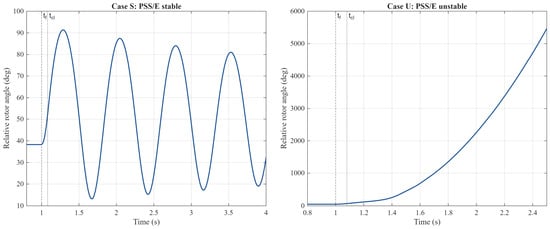
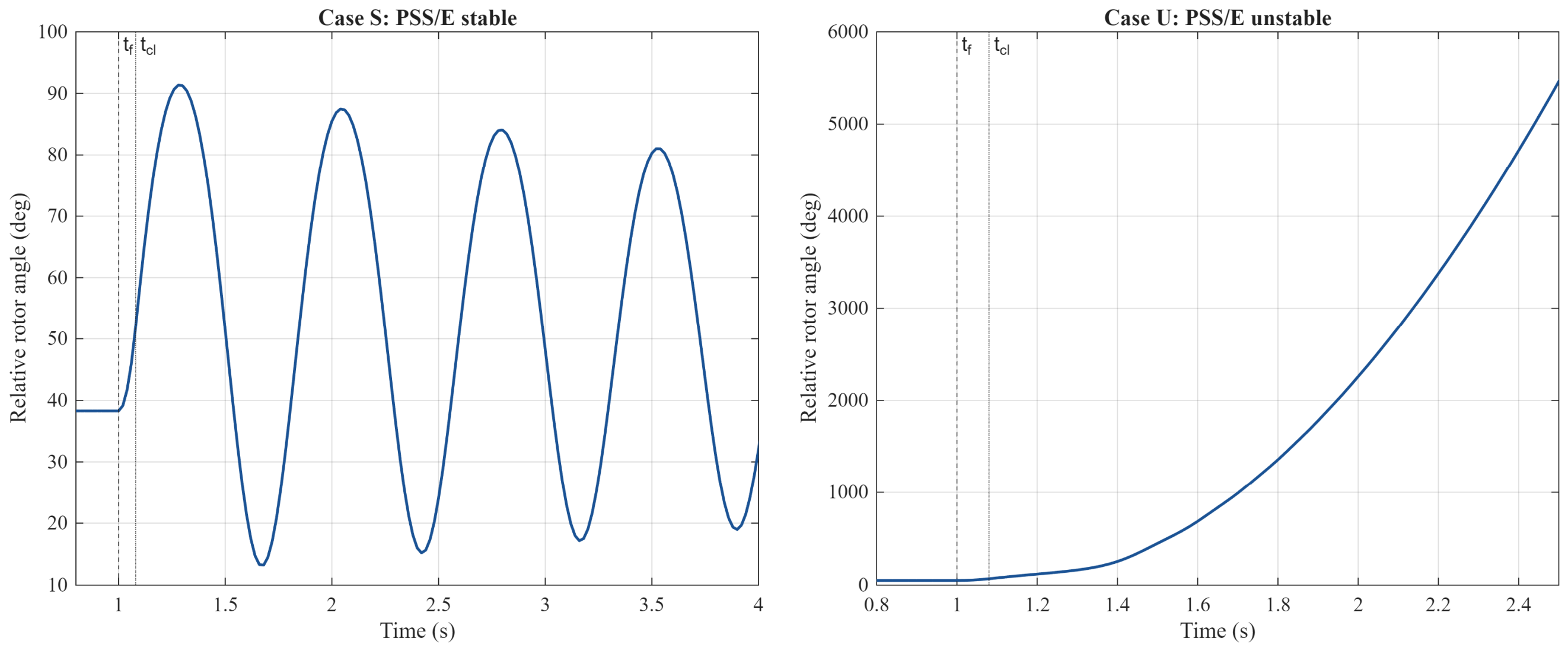
The proposed framework is evaluated in the two operating cases and Figure 4 shows the PSS/E post-fault relative rotor-angle trajectories. For Case S, the normalized MEE index is E_N = 0.5925 < 1, yielding a correct stable decision. For Case U, the normalized MEE index is E_N = 2.2922 > 1, yielding a correct unstable decision. The assessment results in both cases agree with the PSS/E trajectories in Figure 4. Section 3.3, Section 3.4 and Section 3.5 further examine the EKF state estimates, CoO localization, and first-swing consistency of the mirror-equivalent representation.

Figure 4. PSS/E relative rotor angle for Case S and Case U.

3.3. EKF State-Estimation Accuracy

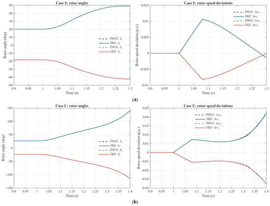
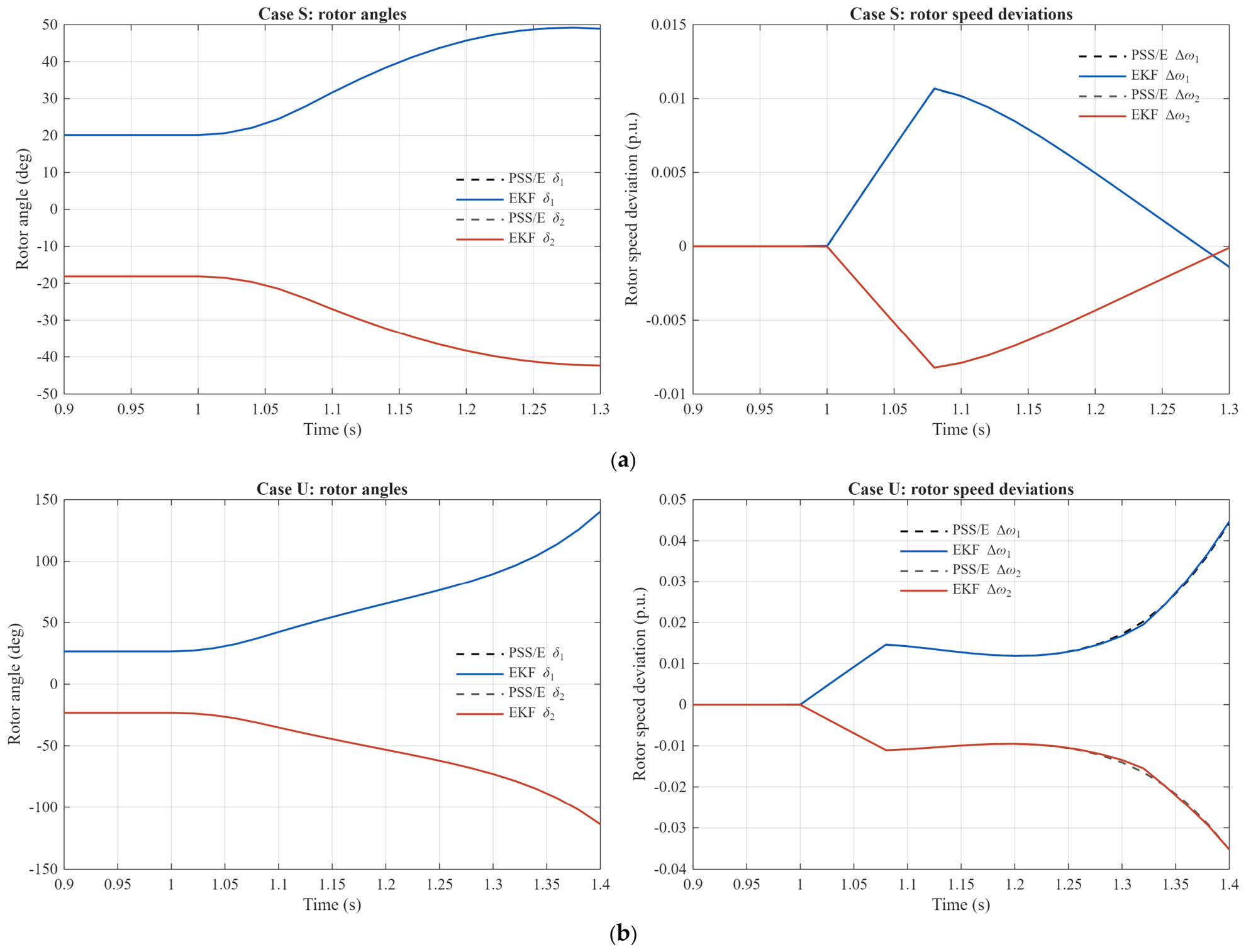
Figure 5 compares the EKF-estimated rotor angles and speed deviations with the corresponding PSS/E results for Cases S and U. The estimated trajectories closely follow the PSS/E results in both cases. The corresponding RMSEs are summarized in Table 2.

Figure 5. Comparison of EKF-estimated rotor angles and speed deviations with PSS/E results: (a) Case S; (b) Case U.

Table 2. RMSEs of the EKF-estimated rotor angles and speed deviations.

Case	Rotor Angle RMSE (Δ1)	Rotor Angle RMSE (Δ2)	Rotor Speed Deviation RMSE (Δω1)	Rotor Speed Deviation RMSE (Δω2)
S	1.36 × 10−4 deg	1.06 × 10−4 deg	9.62 × 10−6 p.u.	6.24 × 10−6 p.u.
U	1.56 × 10−2 deg	1.06 × 10−2 deg	2.38 × 10−4 p.u.	2.88 × 10−4 p.u.

3.4. Virtual-Node-Based CoO Localization

After obtaining the EKF state estimates, the proposed framework reconstructs the frequencies at the virtual nodes and calculates the CoO location using the method described in Section 2.3. To validate the CoO localization, the location calculated from the reconstructed virtual-node frequencies is compared with a reference location obtained by applying the same linear-regression criterion to the PSS/E internal-node frequency trajectories over the same observation window. As shown in Table 3, the estimated CoO locations are 226.067 km from bus M for Case S and 194.786 km from bus M for Case U, whereas the corresponding PSS/E reference locations are 222.786 km and 195.135 km. The absolute errors are therefore 3.281 km and 0.349 km, respectively.

Table 3. Comparison of virtual-node-based CoO locations with PSS/E references.

Case	Reference CoO Location (km)	Virtual-Node-Based CoO Location (km)	CoO Location Absolute Error (km)
S	222.786	226.067	3.281
U	195.135	194.786	0.349

3.5. First-Swing Equivalence of the Mirror System

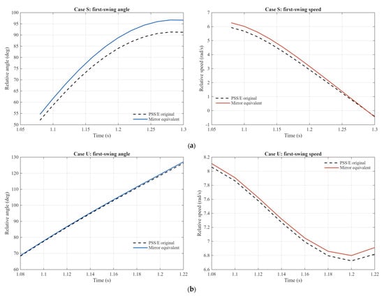
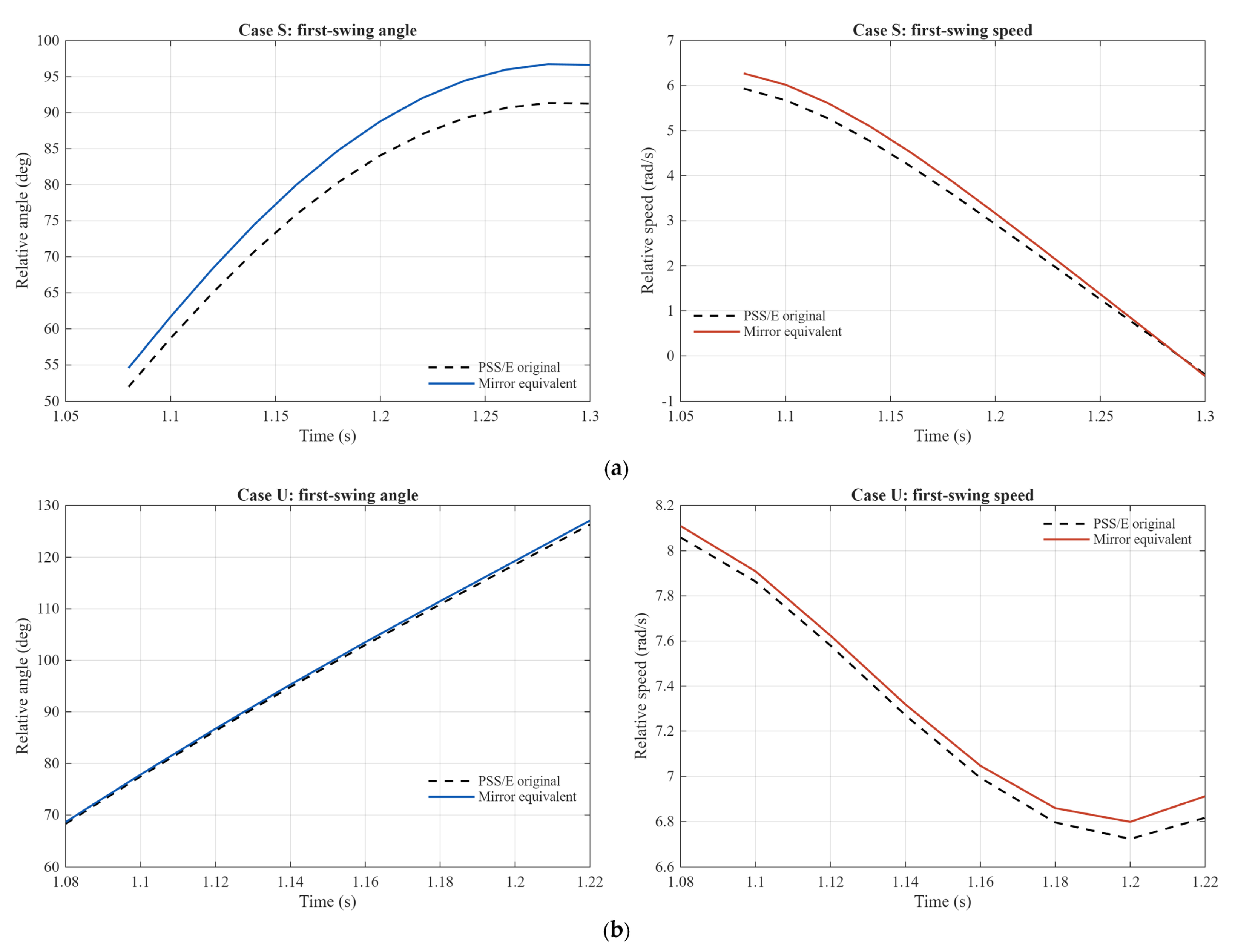
After locating the CoO, the proposed framework calculates the mirror-equivalent relative rotor angle and speed from the EKF state estimates and the reconstructed CoO states. Since the MEE criterion is intended for first-swing stability assessment, these quantities are compared with the corresponding relative states of the original PSS/E two-machine system over the intervals shown in Figure 6. For Case S, the relative-angle and relative-speed RMSEs over the evaluated interval are 4.455° and 0.250 rad/s, respectively. For Case U, the corresponding RMSEs are 0.547° and 0.062 rad/s. These results show that the reconstructed mirror-equivalent states approximately follow the original relative states over the evaluated intervals, supporting their use in first-swing MEE assessment.

Figure 6. Comparison of the first-swing relative rotor angle and speed between the original PSS/E two-machine system and the mirror-equivalent representation: (a) Case S; (b) Case U.

3.6. Comparison with Two-Terminal Interpolation

To evaluate the improvement provided by the virtual-node method, its CoO localization results are compared with those obtained using the conventional two-terminal interpolation method [19] under the same conditions. To ensure a fair comparison, the EKF state estimates and CoO localization procedure are kept the same for both methods. The only difference is the spatial frequency representation: the conventional two-terminal interpolation method calculates the CoO using only the frequencies at the two terminals, whereas the proposed method reconstructs the internal virtual-node frequencies before locating the CoO.

For Cases S and U, the two-terminal interpolation method calculates the CoO locations as 217.550 km and 130.114 km from bus M, respectively. Compared with the PSS/E reference locations shown in Table 3, the corresponding errors are 5.236 km and 65.021 km. By comparison, the virtual-node-based errors in Table 3 are 3.281 km and 0.349 km, representing error reductions of 37.34% and 99.46%, respectively. These results show that the virtual-node method provides more accurate CoO localization than two-terminal interpolation for both cases.

3.7. Comparison with WLS Under Noisy PMU Measurements

Measurement noise may cause large errors in WLS state estimates, which can reduce CoO localization accuracy and may even lead to an incorrect stability decision [22,23,24,25]. To evaluate the improvement provided by EKF-based state estimation across different noise realizations, a Monte Carlo comparison is conducted for Cases S and U at SNRs of 40 and 30 dB. Fifty independent zero-mean Gaussian noise realizations are generated for each Case/SNR combination. Noise is added to the terminal voltage and current phasors and terminal frequencies, with the specified SNR referenced to the demeaned signal power of each channel. In each realization, EKF and conventional WLS use the same noisy PMU measurements and consistent measurement-variance settings, while the virtual-node reconstruction, CoO localization, and MEE calculation procedures remain unchanged.

Table 4 summarizes the mean and sample standard deviation of the absolute CoO location errors, together with the numbers of incorrect stability results. As shown in Table 4, EKF produces smaller mean CoO location errors than WLS for all Case/SNR combinations. All 200 EKF-based MEE decisions agree with the PSS/E results. In contrast, WLS produces one false-unstable decision for Case S at 30 dB. For Case U, it produces two false-stable decisions at 40 dB and four at 30 dB. These results show that EKF improves CoO localization accuracy across repeated noise realizations and provides more reliable MEE decisions under the tested noise conditions.

Table 4. Monte Carlo comparison of EKF and WLS under noisy PMU measurements.

Case	SNR (dB)	Estimator	CoO Absolute Error: Mean ± Standard Deviation (km)	Incorrect Stability Decisions
S	40	WLS	27.143 ±1.818	0/50
S	40	EKF	3.553 ± 1.192	0/50
S	30	WLS	29.791 ± 3.395	1/50
S	30	EKF	4.259 ± 1.718	0/50
U	40	WLS	39.025 ± 2.904	2/50
U	40	EKF	1.675 ± 1.123	0/50
U	30	WLS	44.218 ± 3.517	4/50
U	30	EKF	2.369 ± 1.250	0/50

4. Discussion

This section examines the performance of the proposed method under different operating conditions, the effect of line discretization, computational feasibility, and applicability and limitations.

4.1. Assessment Under Different Operating Conditions

To evaluate the proposed framework beyond the two representative cases, additional simulations are performed using pre-fault transfer powers of 1500, 1790, and 2200 MW. The fault locations are 45, 150, and 255 km from Bus M. Three-phase, single-line-to-ground, and line-to-line faults are considered, with fault durations of 60 and 100 ms. All faults occur on Circuit 1 at 1.00 s. Circuit 1 is disconnected in all three phases at fault clearing, while Circuit 2 remains energized. These combinations produce 54 operating conditions, and all 54 stability decisions agree with the PSS/E results. Due to space limitations, representative results covering different pre-fault transfer powers, fault locations, fault types, and fault durations are summarized in Table 5, which demonstrate that the proposed framework provides correct stability decisions under different operating conditions.

Table 5. Stability-assessment results under different operating conditions.

Pre-Fault Transfer Power (MW)	Fault Type	Fault Location (km)	Fault Duration (ms)	EN	MEE Decision	PSS/E Result	Correct Decision
1500	ABC	255	100	0.3429	Stable	Stable	Yes
1500	A–G	255	60	0.0248	Stable	Stable	Yes
1500	A–G	255	100	0.3161	Stable	Stable	Yes
1500	B–C	255	100	0.0259	Stable	Stable	Yes
1790	ABC	45	100	1.3188	Unstable	Unstable	Yes
1790	ABC	150	100	1.2104	Unstable	Unstable	Yes
1790	ABC	255	60	0.2736	Stable	Stable	Yes
1790	ABC	255	100	1.4458	Unstable	Unstable	Yes
2200	ABC	255	100	1.6142	Unstable	Unstable	Yes
2200	A–G	255	100	0.5734	Stable	Stable	Yes
2200	B–C	255	60	0.7555	Stable	Stable	Yes
2200	B–C	255	100	1.1454	Unstable	Unstable	Yes

4.2. Effect of the Number of Line Sections

Increasing the number of π-sections provides a finer approximation of the distributed-parameter line model but also increases the size of the reconstruction network. Therefore, the selection should consider both numerical accuracy and computational cost. To quantify the line-model approximation error, the overall ABCD matrix obtained by cascading N equal π-sections is compared with that of the analytical distributed-parameter line model at the nominal frequency. Using the elementwise relative-error definition in [26], the maximum relative error among the four ABCD parameters is calculated as

$${\epsilon }_N=100\underset{q\in \{A,B,C,D\}}{\max } {\displaystyle \frac{\left|q_N-q_{\mathrm{d}}\right|}{\left|q_{\mathrm{d}}\right|}}$$

where q_N and q_d denote the corresponding ABCD parameters of the cascaded π-section model and the distributed-parameter model, respectively. For the studied 300 km line, the errors are 0.01804%, 0.00451%, and 0.00200% for 10, 20, and 30 sections, respectively. These results show that increasing the number of sections reduces the line-model approximation error.

To evaluate the effect of line discretization on CoO localization accuracy and computational cost, Cases S and U are tested under noiseless conditions using 10, 20, and 30 sections, corresponding to 9, 19, and 29 internal virtual nodes. The EKF state estimates, observation window, and PSS/E references are kept unchanged. Since EKF processing is common to all configurations, the timing comparison covers only virtual-node reconstruction, CoO localization, and MEE assessment. Table 6 summarizes the CoO location errors and the median post-EKF computation times obtained from 100 repeated runs.

Table 6. Effect of the number of line sections on CoO localization accuracy and computational cost.

Case	π-Sections (Internal Virtual Nodes)	CoO Location Error (km)	Post-EKF Computation Time (ms)
S	10 (9)	3.295	2.35
S	20 (19)	3.281	2.38
S	30 (29)	3.276	2.47
U	10 (9)	0.408	2.22
U	20 (19)	0.349	2.33
U	30 (29)	0.346	2.45

As shown in Table 6, increasing the number of sections from 10 to 20 reduces the CoO location errors by 0.014 km for Case S and 0.059 km for Case U. Further refinement to 30 sections provides additional reductions of only 0.005 km and 0.003 km, respectively. Thus, refinement beyond 20 sections provides limited additional benefit while slightly increasing the computation time. Together with the small ABCD-matrix approximation error, these results support the adopted 20-section representation as a practical resolution for the studied system.

4.3. Computational Feasibility of Online Implementation

The real-time implementation of a DSE-enabled mirror-equivalent energy assessment scheme has been reported in [19], including its installation at a NYPA substation using DFR-PMU streaming data. Its dynamic state estimator requires approximately 0.5 ms per update for a typical substation, and the stability-monitoring scheme operates at 60 updates/s. This field deployment provides a practical precedent for integrating WLS-based dynamic state estimation, CoO localization, and mirror-equivalent energy assessment. It also suggests that PMU reporting and communication delays can be accommodated through appropriate system design. The proposed framework follows this general structure while employing EKF-based state estimation and introducing virtual-node frequency reconstruction.

To evaluate the computational feasibility of the proposed framework, continuous measurement records are processed at 50 frames/s. EKF state estimation and virtual-node frequency reconstruction are performed as each measurement frame arrives, with mean processing times of 0.696 ms and 0.060 ms per frame, respectively. The combined processing time averages 0.757 ms, approximately 3.8% of the 20 ms measurement interval. After the post-fault observation window ends, CoO localization and complete MEE assessment together take approximately 2.14 ms on average. Together with the implementation precedent in [19], these results support the computational feasibility of the proposed framework for online transient stability assessment under the tested conditions.

4.4. Applicability and Limitations

This study presents the theoretical formulation of the proposed framework and demonstrates its effectiveness through simulation studies. However, the framework’s performance in practical systems still requires field validation. Field tests are therefore needed to evaluate stability-assessment accuracy, robustness under practical PMU measurement noise, and end-to-end assessment latency.

The proposed framework is motivated by the stability-monitoring requirements of the Northwest China Power Grid and is evaluated using the studied 750 kV transmission line model. Further validation is required as future work to determine whether the demonstrated performance can be extended to other power grids with different network configurations and operating conditions.

5. Conclusions

This paper has proposed a virtual-node-enhanced MEE framework for the online transient stability assessment of long-distance EHV transmission lines. The main contribution is the use of network-based virtual-node frequency reconstruction to improve CoO localization in long EHV lines and its integration with mirror-equivalent energy assessment. Compared with the conventional two-terminal frequency interpolation method, the proposed framework provides more accurate CoO localization for both stable and unstable cases. The MEE index also yields correct stability decisions for both cases. In addition, the Monte Carlo results at SNRs of 40 and 30 dB show that EKF produces smaller mean CoO location errors and more reliable stability decisions than WLS under the tested conditions. In summary, the proposed framework improves the accuracy of CoO localization and the reliability of online transient stability assessment for the long-distance 750 kV transmission lines. The present validation is limited to simulations of the studied 750 kV system. Future work will include field validation of assessment accuracy, robustness under practical PMU measurement noise, and end-to-end latency, together with evaluation in other grids and network configurations.

References

- Glover, J.D.; Overbye, T.J.; Sarma, M.S. Power System Analysis and Design, 6th ed.; Cengage Learning: Boston, MA, USA, 2017. [Google Scholar]
- Northwest China Energy Regulatory Bureau; National Energy Administration of China. Annual Interprovincial Electricity Exchange in the Northwest China Power Grid Exceeds 60 TWh for the First Time. 2026. Available online: https://xbj.nea.gov.cn/dtyw/hyxx/202601/t20260119_294378.html (accessed on 25 September 2026).
- Hatziargyriou, N.; Milanovic, J.; Rahmann, C.; Ajjarapu, V.; Canizares, C.; Erlich, I.; Hill, D.; Hiskens, I.; Kamwa, I.; Pal, B.; et al. Definition and Classification of Power System Stability—Revisited & Extended. IEEE Trans. Power Syst. 2021, 36, 3271–3281. [Google Scholar] [CrossRef] [Scilit]
- Kundur, P. Power System Stability and Control; McGraw-Hill: New York, NY, USA, 1994. [Google Scholar]
- Anderson, P.M.; Fouad, A.A. Power System Control and Stability, 2nd ed.; Wiley-IEEE Press: Hoboken, NJ, USA, 2003. [Google Scholar]
- Li, B.; Wu, J. Adaptive Assessment of Power System Transient Stability Based on Active Transfer Learning with Deep Belief Network. IEEE Trans. Autom. Sci. Eng. 2023, 20, 1047–1058. [Google Scholar] [CrossRef] [Scilit]
- Ren, C.; Xu, Y.; Zhang, R. An Interpretable Deep Learning Method for Power System Transient Stability Assessment via Tree Regularization. IEEE Trans. Power Syst. 2022, 37, 3359–3369. [Google Scholar] [CrossRef] [Scilit]
- Yu, J.J.Q.; Hill, D.J.; Lam, A.Y.S.; Gu, J.; Li, V.O.K. Intelligent Time-Adaptive Transient Stability Assessment System. IEEE Trans. Power Syst. 2018, 33, 1049–1058. [Google Scholar] [CrossRef] [Scilit]
- Ren, C.; Xu, Y.; Dai, B.; Zhang, R. An Integrated Transfer Learning Method for Power System Dynamic Security Assessment of Unlearned Faults with Missing Data. IEEE Trans. Power Syst. 2021, 36, 4856–4859. [Google Scholar] [CrossRef] [Scilit]
- Xu, Y.; Dong, Z.Y.; Meng, K.; Zhang, R.; Wong, K.P. Real-Time Transient Stability Assessment Model Using Extreme Learning Machine. IET Gener. Transm. Distrib. 2011, 5, 314–322. [Google Scholar] [CrossRef] [Scilit]
- Liu, J.; Liu, J.; Yan, R.; Ding, T. Deep Lyapunov Learning: Embedding the Lyapunov Stability Theory in Interpretable Neural Networks for Transient Stability Assessment. IEEE Trans. Power Syst. 2024, 39, 7437–7440. [Google Scholar] [CrossRef] [Scilit]
- Ma, B.; Yang, J.; Peng, X.; Jiang, K.; Liu, D.; Cao, K. An adaptive assessment method of power system transient stability considering PMU data loss. IET Gener. Transm. Distrib. 2024, 18, 4116–4133. [Google Scholar] [CrossRef] [Scilit]
- Athay, T.; Podmore, R.; Virmani, S. A Practical Method for the Direct Analysis of Transient Stability. IEEE Trans. Power Appar. Syst. 1979, PAS-98, 573–584. [Google Scholar] [CrossRef] [Scilit]
- Tsolas, N.A.; Arapostathis, A.; Varaiya, P.P. A Structure Preserving Energy Function for Power System Transient Stability Analysis. IEEE Trans. Circuits Syst. 1985, CAS-32, 1041–1049. [Google Scholar] [CrossRef] [Scilit]
- Chiang, H.-D.; Wu, F.F.; Varaiya, P.P. A BCU Method for Direct Analysis of Power System Transient Stability. IEEE Trans. Power Syst. 1994, 9, 1194–1208. [Google Scholar] [CrossRef] [Scilit]
- Xue, Y.; Van Cutsem, T.; Ribbens-Pavella, M. A Simple Direct Method for Fast Transient Stability Assessment of Large Power Systems. IEEE Trans. Power Syst. 1988, 3, 400–412. [Google Scholar] [CrossRef] [Scilit] [PubMed]
- Bhui, P.; Senroy, N. Real-Time Prediction and Control of Transient Stability Using Transient Energy Function. IEEE Trans. Power Syst. 2017, 32, 923–934. [Google Scholar] [CrossRef] [Scilit]
- Liu, C.-C.; Vaidya, U.; Meliopoulos, A.P.S. Real Time PMU-Based Stability Monitoring; Final Project Report, PSERC Publication 14-11; Power Systems Engineering Research Center: Tempe, AZ, USA, 2014; Available online: https://pserc.wisc.edu/wp-content/uploads/sites/755/2018/08/S-50_Final-Report-Oct-2014.pdf (accessed on 25 September 2026).
- Farantatos, E.; Huang, R.; Cokkinides, G.J.; Meliopoulos, A.P. A Predictive Generator Out-of-Step Protection and Transient Stability Monitoring Scheme Enabled by a Distributed Dynamic State Estimator. IEEE Trans. Power Deliv. 2016, 31, 1826–1835. [Google Scholar] [CrossRef] [Scilit]
- Milano, F.; Ortega, Á. Frequency Divider. IEEE Trans. Power Syst. 2017, 32, 1493–1501. [Google Scholar] [CrossRef] [Scilit]
- Milano, F.; Ortega Manjavacas, Á. Frequency Variations in Power Systems: Modeling, State Estimation, and Control; Wiley: Hoboken, NJ, USA, 2020. [Google Scholar]
- Monticelli, A. State Estimation in Electric Power Systems: A Generalized Approach; Kluwer Academic Publishers: Boston, MA, USA, 1999. [Google Scholar]
- Chakrabarti, S.; Kyriakides, E. PMU Measurement Uncertainty Considerations in WLS State Estimation. IEEE Trans. Power Syst. 2009, 24, 1062–1071. [Google Scholar] [CrossRef] [Scilit]
- Phadke, A.G.; Thorp, J.S. Synchronized Phasor Measurements and Their Applications; Springer: New York, NY, USA, 2008. [Google Scholar]
- Zhao, J.; Tan, J.; Wu, L.; Zhan, L.; Yao, W.; Liu, Y. Impact of the Measurement Errors on Synchrophasor-Based WAMS Applications. IEEE Access 2019, 7, 143960–143972. [Google Scholar] [CrossRef] [Scilit]
- Ootomo, H.; Ozaki, K.; Yokota, R. DGEMM on integer matrix multiplication unit. Int. J. High Perform. Comput. Appl. 2024, 38, 297–313. [Google Scholar] [CrossRef] [Scilit]
Disclaimer/Publisher’s Note: The statements, opinions and data contained in all publications are solely those of the individual author(s) and contributor(s) and not of MDPI and/or the editor(s). MDPI and/or the editor(s) disclaim responsibility for any injury to people or property resulting from any ideas, methods, instructions or products referred to in the content. |
© 2026 by the authors. Licensee MDPI, Basel, Switzerland. This article is an open access article distributed under the terms and conditions of the Creative Commons Attribution (CC BY) license.