Sub-Synchronous and Super-Synchronous Oscillation Propagation in Offshore Wind Farms with Hybrid DRU MMC HVDC Transmission

Abstract

Hybrid high-voltage direct-current (HVDC) transmission using a diode rectifier unit (DRU) and a modular multilevel converter (MMC) reduces the required capacity of the controllable offshore converter. However, the different terminal controls and AC/DC frequency coupling complicate the assessment of oscillation propagation. This paper presents an impedance-based framework for voltage and current propagation in an offshore wind farm connected through an AC-parallel/DC-series DRU-MMC link. The receiving-end MMC impedance is combined with the series DC network and incorporated into the sending-end hybrid-converter model. Four amplitude ratios characterize AC-to-DC and DC-to-AC propagation while retaining the coupled AC sidebands. In a 1000 MW, 500 kV simulation case, a power increase from 0.4 to 0.5 p.u. produces AC components at 8.3 and 91.7 Hz and a corresponding DC component at 41.7 Hz. With the two AC voltage amplitudes combined by their root-sum-square (RSS), the sending-end AC-to-DC, DC-network, and receiving-end DC-to-AC voltage–amplitude ratios calculated from the reported FFT amplitudes are 0.1474 (−16.63 dB), 0.7648 (−2.33 dB), and 0.2373 (−12.50 dB), respectively. These results support the predicted attenuation trend along the AC–DC–AC path and provide a basis for coordinated terminal monitoring and further damping analysis.

1. Introduction

High-voltage direct-current (HVDC) transmission is an option for connecting large offshore wind farms over long submarine distances. Although a full-scale modular multilevel converter (MMC) provides controllable power conversion and offshore AC-voltage support, the offshore station adds equipment mass, footprint, losses, and cost. Reducing the capacity of the controllable offshore converter therefore motivates the development of hybrid rectifier arrangements [1,2].

A diode rectifier unit (DRU) offers a passive power-conversion path, but it cannot independently establish offshore AC voltage and frequency. These functions must be provided by appropriately controlled wind turbines or a controllable auxiliary converter [3,4,5]. Hybrid arrangements combine the DRU with a voltage-source converter or a full-bridge MMC to improve operating flexibility [6,7,8]. Related station- and converter-level configurations distribute power-conversion and voltage-support duties between the passive and controllable units [9,10,11]. In the configuration studied here, the DRU and sending-end MMC share an AC bus and are connected in series on the DC side. The DRU transfers most of the active power, while the MMC establishes the offshore AC voltage and frequency and regulates reactive power.

The resulting system combines wind-turbine controls, DRU commutation, MMC internal dynamics, the DC network, and receiving-grid dynamics. An oscillation associated with the offshore AC interconnection can consequently appear at several AC and DC terminals. The associated frequencies and amplitudes differ between terminals because power conversion translates frequencies and each closed-loop subsystem has a distinct transfer response. Impedance modeling of DR-MMC transmission has already addressed the influence of converter coupling on stability [12]. Modeling of DRU-based grid-forming converters likewise shows why the controls and passive circuit must be considered together [13].

Impedance-based methods describe subsystem interactions at physical ports [14,15]. Modified sequence-domain impedances retain the coupling between AC components separated by twice the fundamental frequency [16], while harmonic-transfer formulations represent the wider periodic dynamics of converter-dominated systems [17]. For offshore wind integration, AC-side MMC-HVDC models [18], DC-side resonance analysis [19], complete wind-turbine models [20], and harmonic-state-space MMC models [21] establish the importance of both controller and internal-energy dynamics. Other studies connect DC-link control to AC impedance [22], examine the equivalence of AC- and DC-side stability assessment [23], and formulate multiport converter models [24,25]. These results provide the modeling basis for calculating responses across converter terminals.

A stability assessment and a propagation assessment answer related but different questions. The former determines whether an interconnection can sustain a growing perturbation; the latter describes the relative terminal responses associated with that perturbation. SSO propagation coefficients have been developed for MMC multi-terminal DC networks [26], and a hierarchical impedance method with an equivalent single-input and single-output representation has been proposed for cascaded hybrid HVDC systems [27]. Mode-specific interaction and damping analysis has also been reported for HVDC-connected offshore wind farms [28,29,30]. Propagation analysis of the AC-parallel/DC-series DRU–MMC configuration requires a sending-terminal model that jointly represents DRU commutation dynamics, MMC circuit and control dynamics, and the shared AC/DC constraints. A terminal representation developed for a pure-MMC station does not capture these hybrid-converter interactions, which must be retained when deriving the voltage and current propagation relations [12].

The present work focuses on voltage and current transfer through an AC-parallel/DC-series DRU-MMC sending terminal, a series DC network, and a receiving MMC. Its contribution is the connection of these terminal responses using consistent frequency mapping and separate voltage and current amplitude ratios.

The main contributions are as follows:

•

An impedance-based model connects the wind-farm AC interface to the sending-end hybrid converter, DC network, and receiving-end MMC. The model retains the receiving-end controls and the coupled AC components needed to trace the AC/DC propagation path.

•

Four propagation coefficients separately describe voltage and current transfer at the two converter terminals. Root-sum-square normalization includes both retained AC sidebands, and the series-network relation completes the voltage-transfer path between the DC terminals.

•

The framework is applied to the frequency responses and power-step case of a 1000 MW system. The analysis links the 8.3/91.7 Hz AC pair to the 41.7 Hz DC component and distinguishes evidence of attenuation from proof of model accuracy or oscillation-source location.

Section 2 describes the topology, control allocation, and frequency mapping. Section 3 establishes the subsystem relations and their interconnection. Section 4 defines the propagation coefficients and their interpretation. Section 5 presents the simulation results and discusses the scope of the conclusions. Section 6 concludes the paper.

2. System Configuration and Frequency-Coupling Mechanism

2.1. System Configuration and Control Allocation

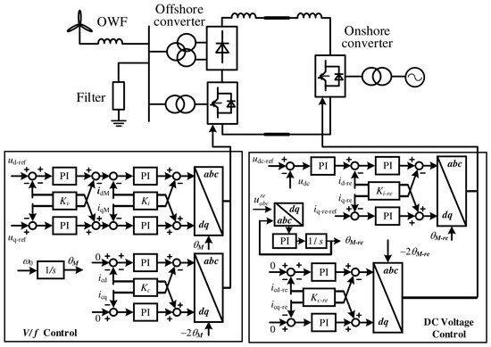
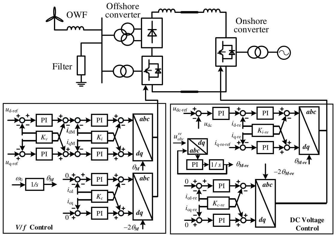
Figure 1 shows the 1000 MW offshore wind transmission system. The wind turbines connect to the offshore AC bus through their grid-side converters, transformers, and collection network. The sending-end hybrid converter consists of a DRU and an MMC connected in parallel on the AC side and in series on the DC side. The DRU carries most of the transmitted active power. The sending-end MMC uses voltage and frequency control, denoted V/f control, to establish the offshore AC bus and provide reactive-power support. The DC connection includes smoothing reactors and a cable. The receiving-end MMC operates as an inverter, regulates the DC voltage, and synchronizes with the onshore AC grid through a phase-locked loop (PLL).

Figure 1. Topology and control allocation of the offshore wind farm connected through the AC-parallel/DC-series hybrid DRU-MMC HVDC system. Arrows indicate the directions of signal flow and control-signal connections.

The hybrid sending station assigns the main active-power rectification duty to the DRU and the offshore AC-voltage and frequency regulation to the MMC. The passive DRU branch carries most of the transmitted active power, reducing the active-power conversion duty of the controllable offshore MMC. The MMC establishes the AC-voltage and frequency reference and provides reactive-power support for the offshore grid. This division of duties combines passive bulk-power rectification with controllable offshore AC-grid operation [6,7,8,12].

In the AC-parallel connection, the DRU and MMC share the offshore-bus voltage, and their branch currents jointly form the terminal AC current. The DC-series connection imposes a common DC current and combines the converter DC voltages according to the series polarity. Consequently, a perturbation can influence both the DRU commutation process and the MMC control response through the shared AC and DC boundaries. The resulting propagation relations must therefore be obtained from the joint DRU–MMC terminal equations, together with the DC-network and receiving-end termination [12].

The system is partitioned at the offshore AC interface and at the DC terminals. The offshore interface connects the aggregated wind-farm impedance to the hybrid-converter impedance. The DC network terminates in the receiving-end MMC impedance. Both voltage and current follow the same physical chain of terminals, but their amplitude-transfer characteristics need not be identical. Throughout the analysis, the DC current is positive from the sending terminal toward the receiving terminal, the sending-end AC current is positive into the hybrid converter, and the receiving-end AC current is positive toward the onshore grid.

2.2. Perturbation Frequency Mapping

Let f₀ = 50 Hz denote the fundamental frequency and f_p the injected positive-sequence AC frequency. In the modified sequence representation, the coupled channel is evaluated at the signed frequency f_p − 2f₀, and the associated DC component is evaluated at f_p − f₀ [16]. The corresponding one-sided spectral frequencies are |f_p − 2f₀| and |f_p − f₀|. Thus, f_p = 91.7 Hz gives a signed companion frequency of −8.3 Hz and a DC frequency of 41.7 Hz; a one-sided AC spectrum displays the companion at 8.3 Hz. Taking an absolute value is only a plotting convention: the sign and associated sequence convention must remain in the model. A one-sided magnitude spectrum alone does not identify sequence direction. The labels “coupled sidebands” are therefore used when discussing the 8.3 and 91.7 Hz spectral peaks.

Here, f₀ denotes the fundamental frequency and f_p represents the positive-sequence AC frequency used to index the propagation calculation. With a 50 Hz fundamental frequency, the synchronous-frame transformation subtracts 50 Hz from the 91.7 Hz AC component, yielding 41.7 Hz. The retained AC/DC coupling channel associates this component with the 41.7 Hz DC ripple. In the modified-sequence representation, a further 50 Hz shift gives a signed companion frequency of −8.3 Hz, which appears at 8.3 Hz in the one-sided spectrum [16]. The two AC components therefore lie 41.7 Hz below and above the fundamental frequency. Physically, these frequencies describe coupled AC sidebands and their associated DC ripple. The shared offshore AC bus couples DRU commutation with MMC control, while the series DC connection links the hybrid-terminal response to the DC network.

Positive- and negative-sequence components at each physical frequency are identified from the complex Fourier phasors of all three phases, using the same observation window and phase reference. With a = exp(j2π/3), the sequence phasors under conventional phase-quantity normalization are X_p(f) = [X_a(f) + aX_b(f) + a²X_c(f)]/3 and X_n(f) = [X_a(f) + a²X_b(f) + aX_c(f)]/3, where X denotes voltage or current.

For real three-phase signals, $X_{\mathrm{n}}(-f)={X_{\mathrm{p}}\left(f\right)}^{*}$, where * denotes complex conjugation. Consequently, the modeled coordinate X_n(−8.3 Hz) corresponds to ${X_{\mathrm{p}}\left(8.3\mathrm{Hz}\right)}^{*}$ when expressed on the positive-frequency axis [16]. Sequence labels must therefore be interpreted together with their signed frequencies. The one-sided magnitude spectra show component frequencies and amplitudes but do not independently establish the physical sequence content.

The model is linearized about a balanced periodic operating point, and it applies to small perturbations. The AC sequence pair retains the principal coupling relevant to the reported oscillation; it is not an exhaustive representation of every commutation or switching sideband. The frequency responses are indexed by the injected AC frequency over the displayed 1–100 Hz interval. In particular, f_p approaching 50 Hz corresponds to a DC perturbation approaching zero frequency, rather than a 50 Hz DC ripple. The exactly zero-frequency limit must be treated separately from a finite-frequency spectral component.

Since f_d = f_p − f₀, an injected AC frequency approaching f₀ corresponds to a slowly varying DC perturbation. At f_p = f₀, the DC increment becomes static and the paired AC coordinates obey real-signal conjugacy. This point requires the incremental equilibrium constraints and consistent DC/AC amplitude conventions when relating the terminal responses.

3. Small-Signal Impedance Modeling

3.1. Receiving-End MMC DC-Side Impedance

The receiving-end MMC employs the PLL-synchronized control scheme shown in Figure 1. The PLL extracts the angle used for the abc-to-dq and dq-to-abc transformations from the receiving-end AC voltage. The outer DC-voltage PI controller generates the d-axis current reference to regulate active-power exchange with the onshore grid, while the q-axis current reference is set to zero. The inner d- and q-axis PI controllers process the current errors and generate the modulation commands together with the cross-coupling compensation terms. Figure 1 also shows a circulating-current suppression branch operating in a reference frame rotating at twice the fundamental frequency. The prefix Δ denotes a small-signal increment; the superscript re denotes a receiving-end quantity. With the independent voltage and current references held constant, the modulation perturbations satisfy

$$\left\{\begin{array}{c}\Delta m_d^{\mathit{re}}=-P_i^{\mathit{re}}(s)\cdot \Delta i_d^{\mathit{re}}-k\cdot \Delta i_q^{\mathit{re}}-P_{\mathit{dc}}(s)P_i^{\mathit{re}}(s)\cdot \Delta u_{\mathit{dc}}^{\mathit{re}}\\ \Delta m_q^{\mathit{re}}=-P_i^{\mathit{re}}(s)\cdot \Delta i_q^{\mathit{re}}+k\cdot \Delta i_d^{\mathit{re}}\end{array}\right.$$

(1)

where $P_i^{re}$ and P_dc denote the current-controller and DC-voltage-controller transfer functions, respectively, and k is the current-loop decoupling coefficient. The controller variables use the normalized scaling of the underlying converter model. Proportional and integral gains enter a PI element as a proportional term plus an integral term divided by the Laplace variable. The PLL relation is

$$\Delta \theta =-H_{\mathit{PLL}}{\displaystyle \frac{1}{s}}\cdot \Delta u_q^{\mathit{re}}$$

(2)

where HPLL represents the PLL regulator preceding the angle integrator. The complete relation from the q-axis voltage increment to the angle increment includes the explicit factor 1/s and the sign convention in (2). The perturbed reference-frame transformations must also be included when connecting the dq controls to the circuit equations. For the upper arm, the linearized circuit relations are

$$\left\{\begin{array}{c}{Z}_{\Delta 1}\Delta i_u^{\mathit{re}}+M_u^{\mathit{re}}\Delta v_u^{\mathit{re}}+V_u^{\mathit{re}}\Delta m_u^{\mathit{re}}+\Delta v_g=\Delta u_{\mathit{dc}}^{\mathit{re}}/2\\ \Delta v_u^{\mathit{re}}=Z_{\Delta c}(M_u^{\mathit{re}}\Delta i_u^{\mathit{re}}+I_u^{\mathit{re}}\Delta m_u^{\mathit{re}})\\ \Delta v_g=Z_g\Delta {\mathrm{i}}_g\end{array}\right.$$

(3)

where the arm-voltage increment represents the equivalent capacitor-voltage sum, and the two impedance operators describe the arm branch and equivalent capacitance. The capitalized arm current, capacitor voltage, and modulation terms denote steady-state quantities. In a harmonic representation, products with periodic steady-state quantities are implemented as harmonic convolution operators, rather than as independent scalar products at a single frequency. The final relation in (3) represents the onshore-grid impedance with its independent source perturbation suppressed. Combining the arm relations, the corresponding lower-arm and phase relations, and the controller and reference-frame equations gives the receiving-end DC terminal response. Its driving-point impedance is defined by

$$Z_r={\displaystyle \frac{\Delta u_{\mathit{dc}}^{\mathit{re}}}{\Delta i_{\mathit{dc}}}}$$

(4)

Equation (4) defines a closed-loop port impedance; its frequency response is obtained only after the internal converter equations have been solved. For a propagation calculation indexed by f_p, this DC impedance and the DC-network impedances are evaluated at the translated DC frequency f_p − f₀. The AC circuit and controller channels are evaluated at their corresponding translated frequencies within the coupled model. This distinction is necessary to avoid evaluating every subsystem at the same numerical frequency. The PLL, DC-voltage loop, and internal MMC dynamics connect the onshore AC conditions to the DC response [19,21,22].

During propagation, a receiving-end DC-voltage perturbation changes the d-axis current reference through the outer voltage loop. The inner current loop subsequently modifies the modulation commands and AC currents, affecting active-power exchange and the converter energy response. This cascaded control action is represented by the product of the DC-voltage and current-controller transfer functions in (1). An AC-voltage perturbation also affects the PLL angle through (2), introducing reference-frame perturbations into the coupled converter equations. Together with the MMC arm and capacitor dynamics, these control paths determine the closed-loop DC impedance in (4). This impedance enters the DC-network relations in (5) and (6) and the receiving-end propagation coefficients in Section 4.2, thereby capturing the frequency-dependent influence of the receiving-end controls on oscillation propagation [19,21,22].

Equations (1)–(4) use a continuous-time representation of the receiving-end controls, retaining the PI regulators and the PLL angle integrator explicitly. Sampling, computational, and modulation delays are neglected in the analytical derivation. The resulting closed-loop terminal impedance and propagation coefficients characterize the converter response under this modeling assumption.

3.2. DC-Network Aggregation

Under the series DC-network representation, the cable and smoothing reactors carry the same perturbation current as the receiving-end DC port. The impedance seen from the sending-end DC terminal is therefore

Z_r−equ = Z_r + Z_DC−line + Z_L

(5)

where the cable term denotes the series impedance of the adopted line approximation, and the reactor term includes the smoothing inductance represented in that series path. Equation (5) assumes that shunt cable-current paths are neglected. It cannot be applied unchanged to a cable represented by a distributed model or a π circuit with retained shunt capacitances; such a network must be reduced together with its receiving-end termination, and the two terminal currents may differ. With the series approximation, the sending-end DC voltage satisfies

$$\Delta u_{\mathit{dc}}^{\mathit{send}}=Z_{r-\mathit{equ}}\cdot \Delta i_{\mathit{dc}}$$

(6)

Equation (6) closes the DC boundary of the hybrid-converter model. Consequently, changes in the receiving-end controller or onshore-grid impedance can affect the sending-end AC response through the DC connection.

3.3. Sending-End Hybrid Converter and Wind-Farm Impedances

The aggregated wind farm is represented by a 2 × 2 sequence-impedance matrix at the offshore interface. Its diagonal elements describe the direct responses of the retained channels and its off-diagonal elements describe frequency coupling. Transformer ratios and collection-network impedances must be referred to this same interface. Wind-turbine converter and DC-link dynamics enter through the selected turbine model [20]. The hybrid-converter impedance is constructed from the coupled sending-end MMC circuit and control equations, the DRU switching and commutation relations, and the DC boundary condition in (6). At the common offshore AC bus, the converter branches share the bus voltage and contribute jointly to the terminal current. On the DC side, the model enforces the common current and the series voltage sum. These boundary conditions couple the DRU commutation response to the sending-end MMC circuit and control dynamics, while the DC-network and receiving-end MMC impedances enter through (6).

The DR-MMC circuit formulation in [12] provides the basis for this part of the model.

The sending-end MMC control effects can be written in the compact form

$$\Delta m_u^{\mathit{se}}=G_i\Delta i_u^{\mathit{se}}+G_v\Delta v_{\mathit{hybird}}$$

(7)

where G_i and G_v are the effective current- and voltage-feedback operators in the arm-modulation relation, and se denotes the sending-end MMC. These operators include the controller interconnection and required coordinate transformations; they are not interchangeable with individual PI gains. Combining the control and circuit relations with (6) yields the hybrid-converter terminal impedance and its inverse admittance. Off-diagonal terms retain the coupling produced by the periodic converter dynamics, including DRU commutation and MMC modulation.

For the impedance-interconnection calculation, a positive-sequence test voltage is represented as a series perturbation source at the interface between the wind-farm and hybrid-converter equivalents. It is distinct from an ideal voltage clamp directly imposed at the hybrid-converter bus. With all other independent source perturbations suppressed, Kirchhoff’s voltage law gives the following terminal responses:

$$\left\{\begin{array}{c}\left[\begin{array}{c}\Delta v_{p-\mathit{hybrid}}\\ \Delta v_{n-\mathit{hybird}}\end{array}\right]=\mathit{inv}(I+Z_{\mathit{WF}}{Y}_{\mathit{hybrid}})\cdot \left[\begin{array}{c}\Delta v_p\\ 0\end{array}\right]\\ \left[\begin{array}{c}\Delta i_{p-\mathit{hybrid}}\\ \Delta i_{n-\mathit{hybird}}\end{array}\right]=Y_{\mathit{hybrid}}\cdot \mathit{inv}(I+Z_{\mathit{WF}}{Y}_{\mathit{hybrid}})\cdot \left[\begin{array}{c}\Delta v_p\\ 0\end{array}\right]\end{array}\right.$$

(8)

where the identity matrix has order two. The first vector contains the actual hybrid-converter terminal-voltage components and the second contains the associated current components. Equation (8) follows from adding the wind-farm impedance drop to the hybrid terminal voltage, with current determined by the hybrid admittance. Matrix multiplication order must be preserved. Although the series test source has only a positive-sequence component, the terminal response generally contains both coupled channels. These terminal quantities, rather than the imposed source amplitude alone, are used in the propagation coefficients.

4. Oscillation Propagation Coefficient Framework

The four propagation coefficients characterize two conversion stages and two physical quantities: voltage and current transfer from offshore AC to sending-end DC, and from receiving-end DC to onshore AC. Separate voltage and current ratios are defined at each stage because their transfer characteristics depend on the terminal impedances. The retained coupled AC components are obtained from the complex terminal-model solution and combined using RSS to define the AC-side amplitudes. Together with the DC-network relations in Section 4.3, these coefficients describe aggregate amplitude propagation along the investigated AC–DC–AC path for the specified operating point and excitation.

4.1. Offshore AC-to-DC Propagation

For the terminal response obtained from (8), the sending-end MMC and DRU equations determine the associated DC perturbations at the translated frequency. The voltage and current amplitude-transfer coefficients are defined as

$$K_{\mathit{AC}-\mathit{DC}}^u={\displaystyle \frac{\Delta u_{\mathit{dc}}^{\mathit{send}}}{\sqrt{{\left|\Delta v_{p-\mathit{hybird}}\right|}^2+{\left|\Delta v_{n-\mathit{hybird}}\right|}^2}}}$$

(9)

$$K_{\mathit{AC}-\mathit{DC}}^i={\displaystyle \frac{\Delta i_{\mathit{dc}}}{\sqrt{{\left|\Delta i_{p-\mathit{hybird}}\right|}^2+{\left|\Delta i_{n-\mathit{hybird}}\right|}^2}}}$$

(10)

Each denominator is the root-sum-square (RSS) magnitude of the two retained AC components. The ratios are independent of the test-signal magnitude within the linear range but depend on the operating point, DC termination, and relative amplitude and phase of the coupled excitation. All voltage and current amplitudes must use consistent peak or RMS conventions and explicitly defined measurement ports. These same-unit ratios are dimensionless but do not remove transformer-ratio or rated-base effects. RSS is the square root of the sum of the squared component magnitudes and is unchanged when their phases change while their magnitudes remain fixed. It therefore discards the relative phase of the retained AC sidebands and cannot reconstruct the instantaneous waveform or its peak. The complex-valued terminal model retains phase information, but the scalar coefficients report only aggregate amplitude transfer; they do not quantify oscillatory power, energy dissipation, or damping. Accordingly, these magnitude ratios alone cannot identify the oscillation source or establish damping performance.

4.2. Onshore DC-to-AC Propagation

At the receiving-end DC terminal, the voltage increment is

$$\Delta u_{\mathit{dc}}^{\mathit{re}}=Z_r\cdot \Delta i_{\mathit{dc}}$$

(11)

The retained upper-arm current components are related to the AC terminal components and common DC-link current by

$$\left\{\begin{array}{c}\Delta i_{p-\mathit{rece}}=2\Delta i_u^{\mathit{re}}(f_p)\\ \Delta i_{n-\mathit{rece}}=2\Delta i_u^{\mathit{re}}(f_p-2f_0)\\ \Delta i_{\mathit{dc}}=3\Delta i_u^{\mathit{re}}(f_p-f_0)\\ \begin{array}{c}\Delta v_{p-\mathit{rece}}=Z_g\cdot \Delta i_{p-\mathit{rece}}\\ \Delta v_{n-\mathit{rece}}=Z_g\cdot \Delta i_{n-\mathit{rece}}\end{array}\end{array}\right.$$

(12)

where the frequency arguments distinguish the retained channels and the factors of two and three follow from the arm-to-phase and balanced three-phase DC-current relations, respectively. The AC-grid impedances must be evaluated at the signed frequencies of their respective channels. The receiving-end voltage and current coefficients are then

$$K_{\mathit{DC}-\mathit{AC}}^u={\displaystyle \frac{\sqrt{{\left|\Delta v_{p-\mathit{rece}}\right|}^2+{\left|\Delta v_{n-\mathit{rece}}\right|}^2}}{\Delta u_{\mathit{dc}}^{\mathit{re}}}}$$

(13)

$$K_{\mathit{DC}-\mathit{AC}}^i={\displaystyle \frac{\sqrt{{\left|\Delta i_{p-\mathit{rece}}\right|}^2+{\left|\Delta i_{n-\mathit{rece}}\right|}^2}}{\Delta i_{\mathit{dc}}}}$$

(14)

The input is the receiving-end DC perturbation and the output is the RSS magnitude of the corresponding AC pair. The argument f_p is retained to align these curves with the sending-end sweep; it is not the frequency of the receiving-end DC excitation. Separate coefficients are needed because the converter and grid impedances give different relations between voltage and current at each frequency.

4.3. Interpretation and Propagation Along the DC Link

Each amplitude coefficient can be expressed in decibels as

$$K_{\mathit{dB}}^x(f)=20{\log }_{10}{K}^x(f),x\in \{u,i\}$$

(15)

For a nonzero denominator, a coefficient above 0 dB denotes a larger output amplitude under the stated normalization, whereas a coefficient below 0 dB denotes a smaller output amplitude. A positive peak alone does not establish an unstable mode, and a negative coefficient does not establish positive damping. Ratios with vanishing denominators require separate treatment and must not be interpreted as finite amplification.

The DC-network segment must also be included when tracing voltage from one AC terminal to the other. Dividing (11) by (6) gives the receiving-to-sending DC-voltage amplitude ratio. For the common-current series representation, the DC-current amplitude ratio is unity:

$$\begin{array}{c}{K}_{\mathit{DC}}^u=\left|{\displaystyle \frac{\Delta u_{\mathit{dc}}^{\mathit{re}}}{\Delta u_{\mathit{dc}}^{\mathit{send}}}}\right|=\left|{\displaystyle \frac{Z_r}{Z_{r-\mathit{equ}}}}\right|\\ K_{\mathit{DC}}^i=1\end{array}$$

(16)

All impedances in (16) are evaluated at the same translated DC frequency. For the same coupled response and consistent amplitude conventions, the complete AC-to-AC amplitude ratios follow by multiplying the successive segment ratios:

$$\begin{array}{c}{K}_{\mathit{path}}^u=K_{\mathit{AC}-\mathit{DC}}^u{K}_{\mathit{DC}}^u{K}_{\mathit{DC}-\mathit{AC}}^u\\ K_{\mathit{path}}^i=K_{\mathit{AC}-\mathit{DC}}^i{K}_{\mathit{DC}-\mathit{AC}}^i\end{array}$$

(17)

The products in (17) are algebraic identities for the same propagated response, rather than independent worst-case gains; coefficients computed for unrelated excitations or operating points cannot be combined this way. The diagnostic procedure is to select an injected AC frequency, solve (8), obtain the corresponding DC and receiving-end arm responses, and evaluate the converter and DC-network ratios. Equation (17) combines the converter propagation coefficients with the DC-network factors in (16) to obtain the end-to-end voltage and current amplitude ratios. The voltage path includes the DC-voltage transfer factor, while the current path uses the unity DC-current factor of the adopted series representation. All segment ratios are evaluated for the same coupled response at the corresponding AC and translated DC frequencies, using consistent terminal definitions and amplitude conventions. Their products therefore account for the successive amplitude changes across the two converters and the intervening DC network. The evaluation proceeds by solving (8), obtaining the associated DC and receiving-end AC responses, and calculating the converter and network amplitude ratios. This provides a compact description of aggregate voltage and current propagation along the modeled path, while the underlying complex terminal model retains the converter–network coupling and phase information.

The four propagation coefficients are evaluated from the same coupled AC/DC response, with the AC amplitudes formed from the retained pair. Near the fundamental frequency, each channel retains its signed frequency argument, including s_d = j2π(f_p − f₀) for the DC channel. For nonzero f_d, the inverse in (8) can be evaluated by factorizing and solving M(f_p)U_ac,se = S, with M = I + Z_WFY_hybrid, followed by I_ac,se = Y_hybridU_ac,se.

Reliable evaluation close to 50 Hz requires consistent scaling, a conditioning estimate, a normalized residual check, and frequency refinement on both sides of the fundamental frequency. At s_d = 0, direct substitution into isolated integral or capacitor impedance terms is invalid; the coupled incremental equilibrium equations must be used, retaining the relevant integral and capacitor states. Whether a finite terminal limit exists must be determined from that coupled system.

The propagation ratios must also be interpreted alongside the absolute terminal amplitudes. A small DC input amplitude can increase a DC-to-AC ratio without a correspondingly large absolute AC response. If a denominator vanishes, the ratio is undefined; any limit must be obtained from the jointly solved response before combining successive propagation stages.

$$\left[\begin{array}{c}{I}_{\mathrm{ac}}\\ I_{\mathrm{dc}}\end{array}\right]=\left[\begin{array}{cc}{Y}_{\mathrm{aa}}& Y_{\mathrm{ad}}\\ Y_{\mathrm{da}}& Y_{\mathrm{dd}}\end{array}\right]\left[\begin{array}{c}{U}_{\mathrm{ac}}\\ U_{\mathrm{dc}}\end{array}\right]$$

(18)

In (8), the positive-sequence-only source is generalized to the complex vector $\mathit{S}={[S_{\mathrm{p}},S_{\mathrm{n}}]}^{\mathrm{T}}$. Solving for the two independent source coordinates gives the direct and cross-sequence response columns while retaining phase throughout the AC/DC path. A negative-sequence excitation at signed frequency f_n is handled with f_d = f_n + f₀ and its paired positive-sequence frequency f_p = f_n + 2f₀. For arbitrary excitations, the corresponding shifted-frequency blocks must be assembled; an unbalanced operating point or additional retained harmonics may require a larger harmonic basis.

For fixed terminations and suppressed independent receiving-grid perturbations, the voltage conversion maps may be expressed as a complex sending-end row operator h_u and a receiving-end column operator g_u. Corresponding current operators use the current port variables and their boundary conditions. These operators are obtained after applying the interconnection constraints; the AC/DC feedback must remain in the solution.

$$\begin{array}{l}{U}_{\mathrm{dc}}^{\mathrm{se}}=h_{\mathrm{u}}^{\mathrm{se}}{U}_{\mathrm{ac}}^{\mathrm{se}}\hfill \\ U_{\mathrm{ac}}^{\mathrm{re}}=g_{\mathrm{u}}^{\mathrm{re}}{U}_{\mathrm{dc}}^{\mathrm{re}}\hfill \end{array}$$

(19)

The entries of g_u give the individual complex DC-to-AC channel transfers. With consistent port and phasor normalization, their RSS norm recovers the receiving-end aggregate voltage coefficient in Section 4.2. At the sending end, the DC response is the coherent sum h_u,p U_p + h_u,n U_n, so its magnitude also depends on the relative phase of the two AC inputs. The four existing scalar coefficients remain aggregate summaries for a specified solved response; individual sequence paths and phase relations require the complex operators.

$$K_{\mathrm{RSS}}^{\mathrm{u}}=\sqrt{{\left|g_{\mathrm{u},\mathrm{p}}^{\mathrm{re}}\right|}^2+{\left|g_{\mathrm{u},\mathrm{n}}^{\mathrm{re}}\right|}^2}$$

(20)

The extension described here specifies how to retain and report sequence information. The present one-sided terminal spectra do not provide a numerical validation of separate sequence transfer operators. Such a comparison requires the synchronized three-phase complex phasors described in Section 2.2.

5. Simulation Results and Discussion

5.1. Test System

The simulations were performed in MATLAB/SimulinkR2024b for the 1000 MW, 500 kV offshore wind-export system. This reference case is used to examine voltage and current oscillation propagation from the offshore AC bus through the hybrid DRU–MMC sending terminal and DC network to the receiving-end MMC. The analytical calculation and time-domain case use the same circuit and controller parameter set. The power, DC-voltage, and DC-current bases are 1000 MW, 500 kV, and 2000 A, respectively, satisfying 500 kV × 2000 A = 1000 MW. The DC smoothing inductance is 0.2 H; the circuit parameters and controller proportional/integral gain pairs are listed in Table 1.

Table 1. Main circuit and controller parameters. Controller gains are proportional/integral pairs.

Parameter	Symbol	Value
Wind-farm rated power	Pnom	1000 MW
Wind-turbine PLL gains	kp-PLL/ki-PLL	0.5/32.7 p.u.
Wind-turbine current-loop gains	kp/ki	0.2/3 p.u.
Rated DC voltage	Udc	500 kV
Rated DC current	Idc	2000 A
Per-unit bases (power/DC voltage/DC current)	Pb/Udc,b/Idc,b	1000 MW/500 kV/2000 A
DC smoothing inductance	Ldc	0.2 H
Sending MMC voltage-loop gains	kpv-s/kiv-s	4/35 p.u.
Sending MMC current-loop gains	kpi-s/kii-s	0.14/30 p.u.
Receiving MMC PLL gains	kp-pll-r/ki-pll-r	0.1/1.3 p.u.
Receiving MMC DC-voltage-loop gains	kp-dc-r/ki-dc-r	4/35 p.u.
Receiving MMC current-loop gains	kpi-r/kii-r	1.1/35 p.u.

For the receiving-end MMC, the normalized proportional/integral gain pairs are 0.1/1.3 for the PLL, 4/35 for the DC-voltage loop, and 1.1/35 for the inner current loops, as specified in Table 1. Each PI regulator is represented as k_p + k_i/s, with the PLL angle integration retained separately in (2). These gains are used as fixed test-system parameters for the investigated power increase.

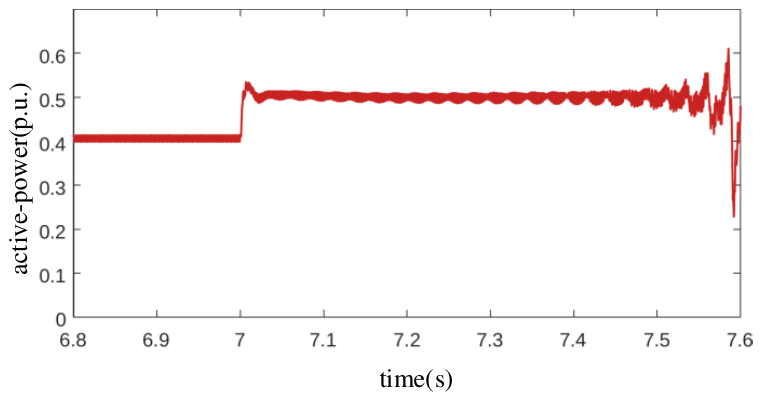
The fundamental frequency is 50 Hz, and the numerical time step is 1 μs throughout the investigated time-domain case. This time step specifies the numerical simulation resolution and is distinct from a physical controller delay. At approximately 7.0 s, wind-farm power increases from 0.4 to 0.5 p.u., corresponding to 400 and 500 MW on the 1000 MW power base. These values specify the operating power levels of the reference system.

The frequency-domain propagation calculation covers positive-sequence AC frequencies of 1–100 Hz, with the coupled AC and DC frequencies defined in Section 2.2. The time-domain power-step case is used to examine the corresponding spectral components and their voltage/current distribution across the terminals. The scope of this comparison and the interpretation of the nonstationary spectra are discussed in Section 5.3 and Section 5.4.

The analytical model is linearized around a balanced periodic operating point, retains the coupled AC/DC channels, and uses a series DC-network approximation that neglects cable shunt-current paths. The control relations follow the continuous-time representation in Section 3.1. The propagation results apply to the stated parameters and operating scenario; analysis at another rating or operating point requires consistent updates to the physical parameters, controller normalization, operating-point model, and terminal impedances.

5.2. Frequency-Sweep Results

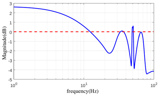
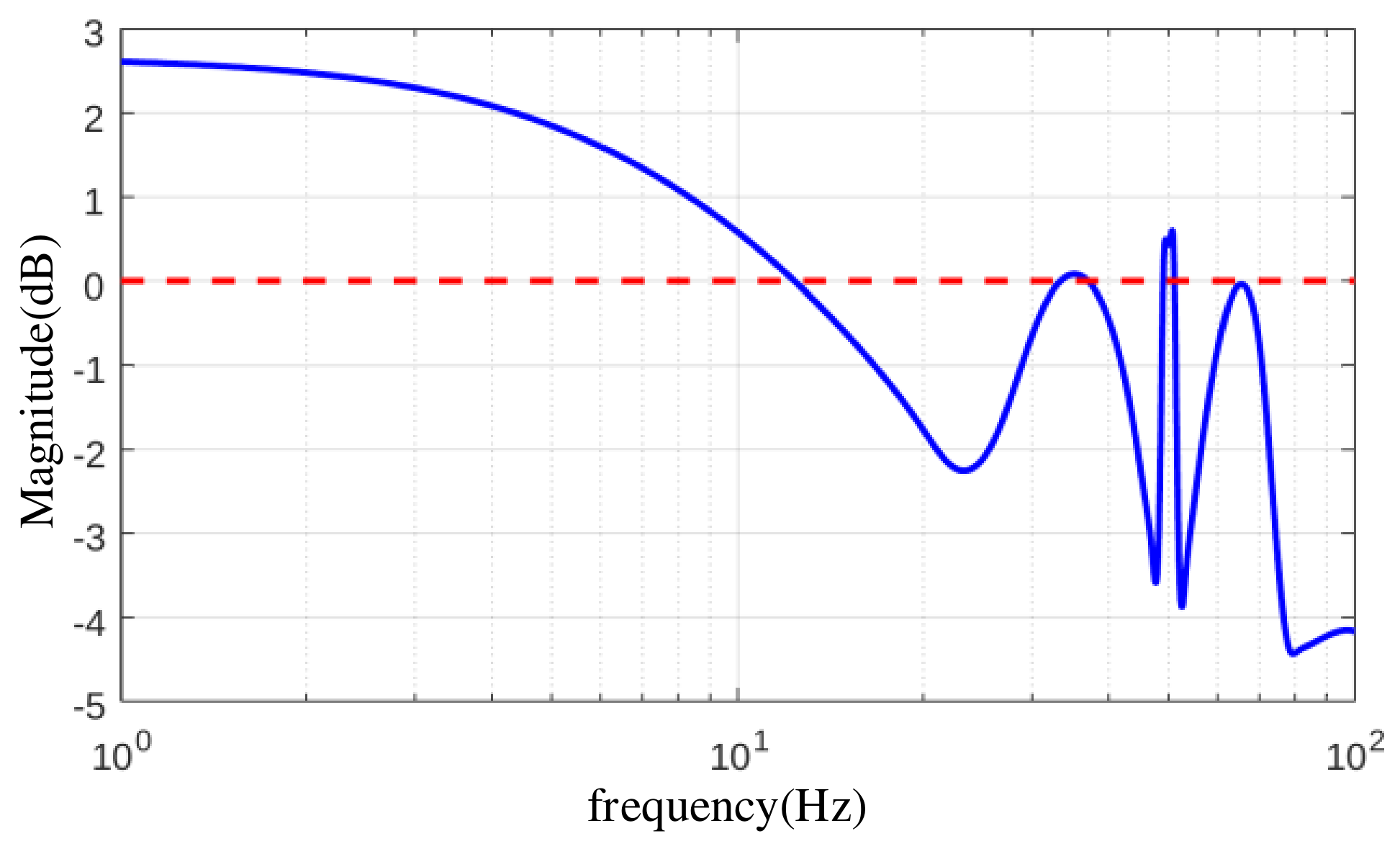
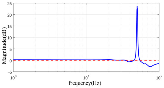
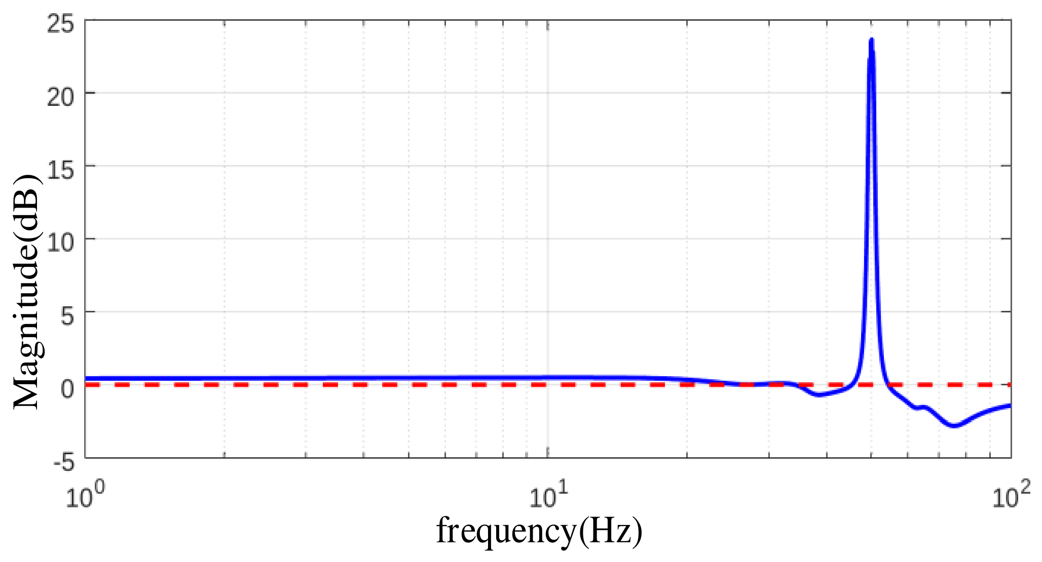
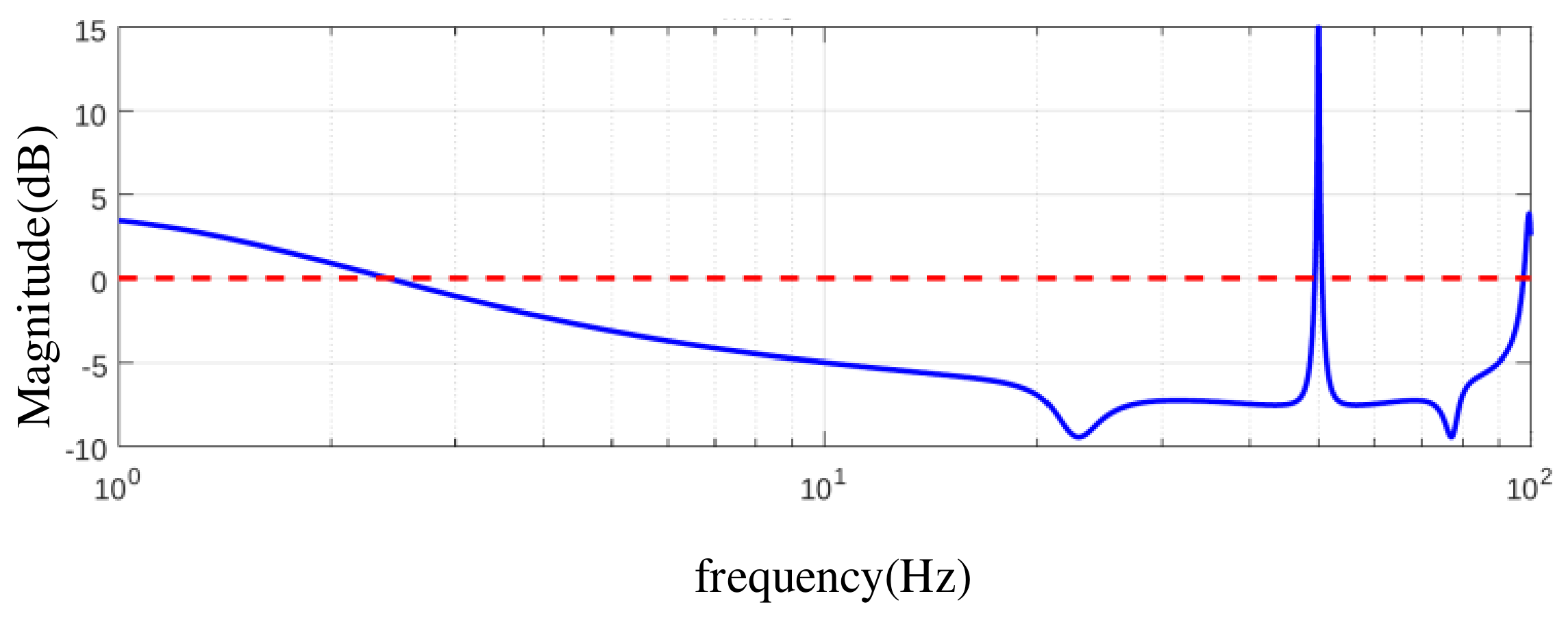
Figure 2 and Figure 3 show the sending-end AC-to-DC current and voltage coefficients. The broad trend in Figure 2 is a transition from low-frequency amplification to predominantly attenuating current transfer above approximately 11 Hz. Narrow local excursions mean that this threshold should not be interpreted as a strict boundary for every frequency. In Figure 3, voltage transfer is close to unity below approximately 40 Hz, exhibits a sharp peak near an injected AC frequency of 50 Hz, and is predominantly attenuating above approximately 55 Hz. The different responses demonstrate why current attenuation alone is insufficient to describe voltage propagation.

Figure 2. Sending-end hybrid-converter AC-to-DC current propagation coefficient in dB versus injected AC frequency f_p. The blue solid curve represents the current propagation coefficient, and the red dashed line indicates the 0 dB reference level.

Figure 3. Sending-end hybrid-converter AC-to-DC voltage propagation coefficient in dB versus injected AC frequency f_p. The blue solid curve represents the voltage propagation coefficient, and the red dashed line indicates the 0 dB reference level.

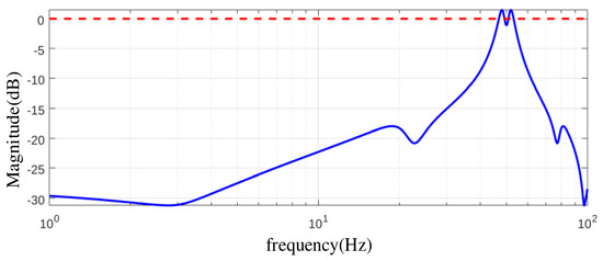
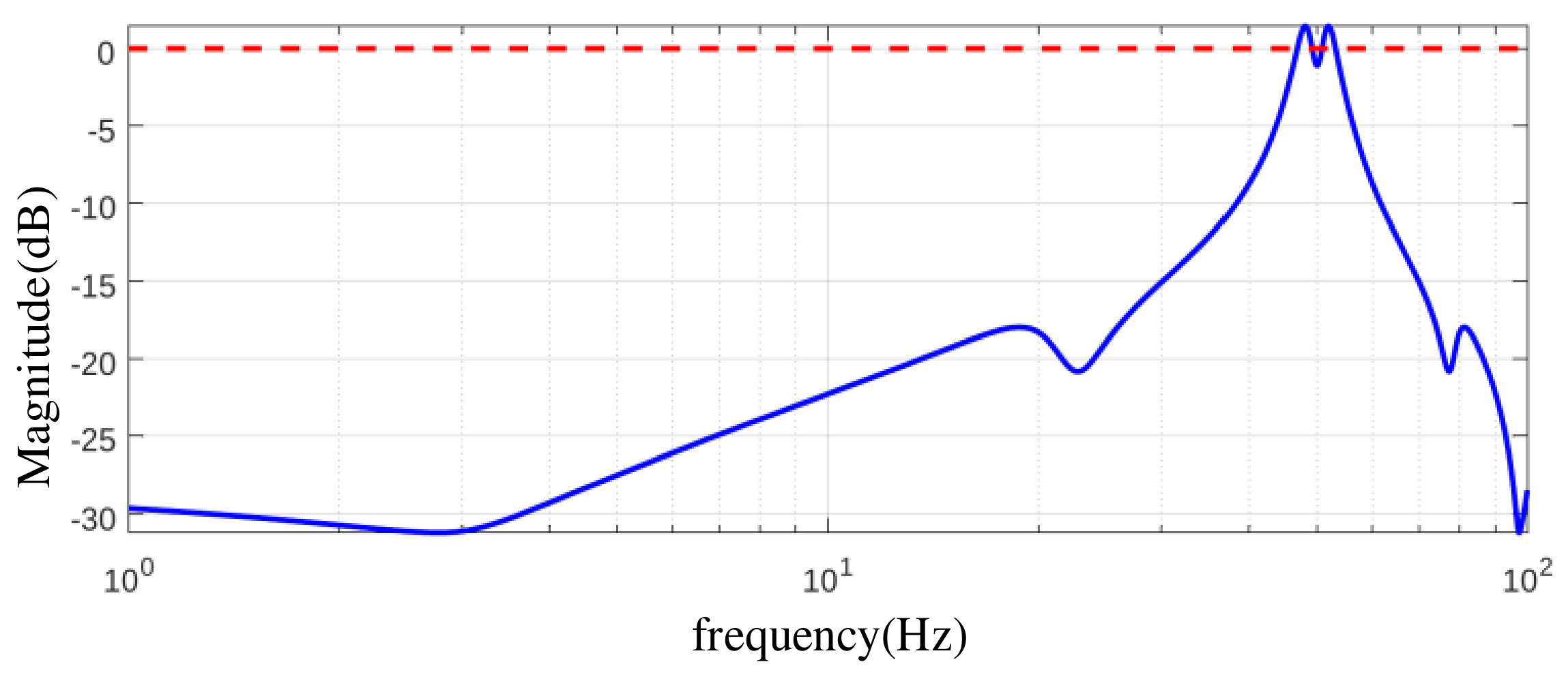
Figure 4 and Figure 5 show the receiving-end DC-to-AC coefficients, indexed by the same injected AC frequency. Current transfer is attenuating over most of the displayed range, with a narrow exception near 50 Hz. Voltage transfer is also attenuating over much of the range, with amplification in the very-low-frequency region and near 50 Hz. Figure 5 additionally rises near the upper end of the plotted interval, so attenuation should not be extrapolated beyond the displayed range. The near-50 Hz region corresponds to a near-zero DC perturbation frequency. Its peaks therefore require examination of the low-frequency converter response and the coefficient denominators; frequency translation by itself is not a damping or instability mechanism.

Figure 4. Receiving-end MMC DC-to-AC current propagation coefficient in dB versus injected AC frequency f_p. The corresponding DC frequency is |f_p − f₀|. The blue solid curve represents the current propagation coefficient, and the red dashed line indicates the 0 dB reference level.

Figure 5. Receiving-end MMC DC-to-AC voltage propagation coefficient in dB versus injected AC frequency f_p. The corresponding DC frequency is |f_p − f₀|. The blue solid curve represents the voltage propagation coefficient, and the red dashed line indicates the 0 dB reference level.

The near-50 Hz peaks characterize the computed amplitude propagation ratios in the low-translated-frequency region. Their physical interpretation requires the coupled-response and normalization checks in Section 4.3; the peaks alone do not establish an unstable mode or a physical resonance. The power-step case at f_p = 91.7 Hz and |f_d| = 41.7 Hz illustrates the propagation pattern away from this limiting region.

5.3. Power Step and Terminal Spectra

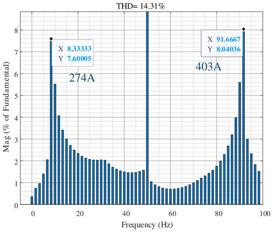
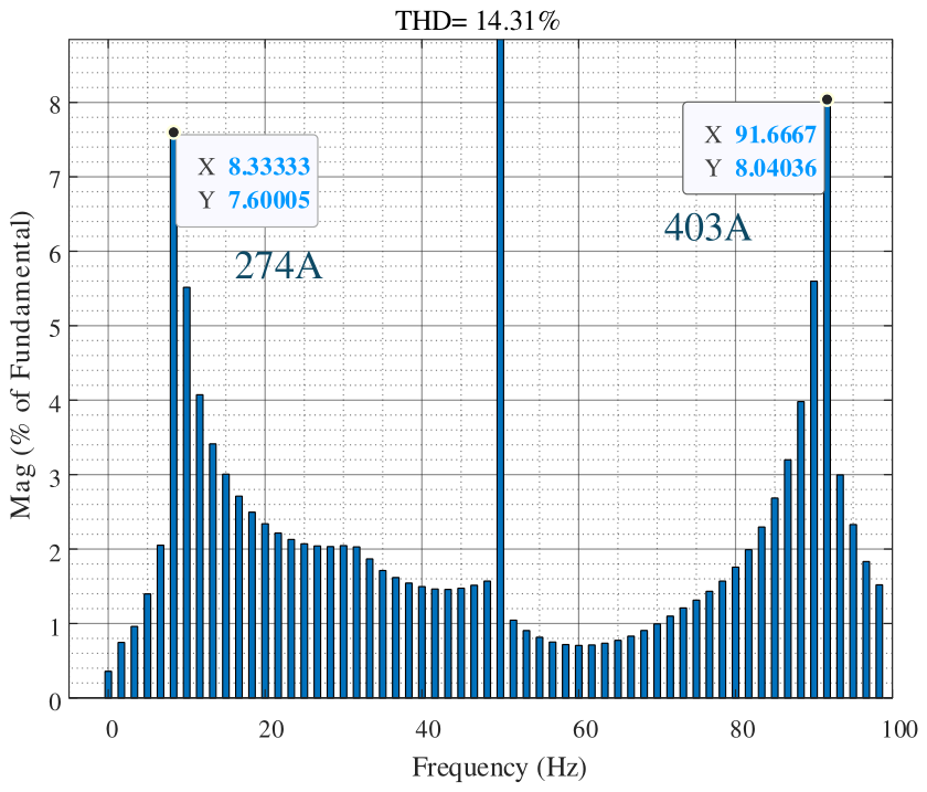
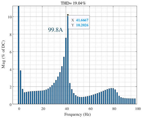
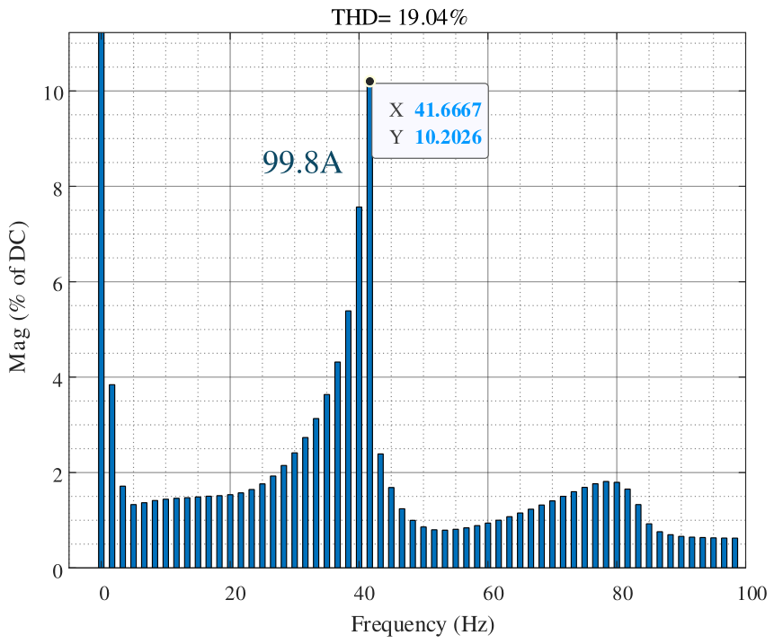
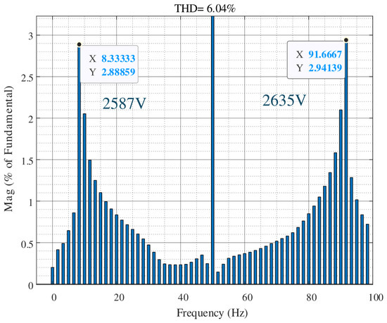
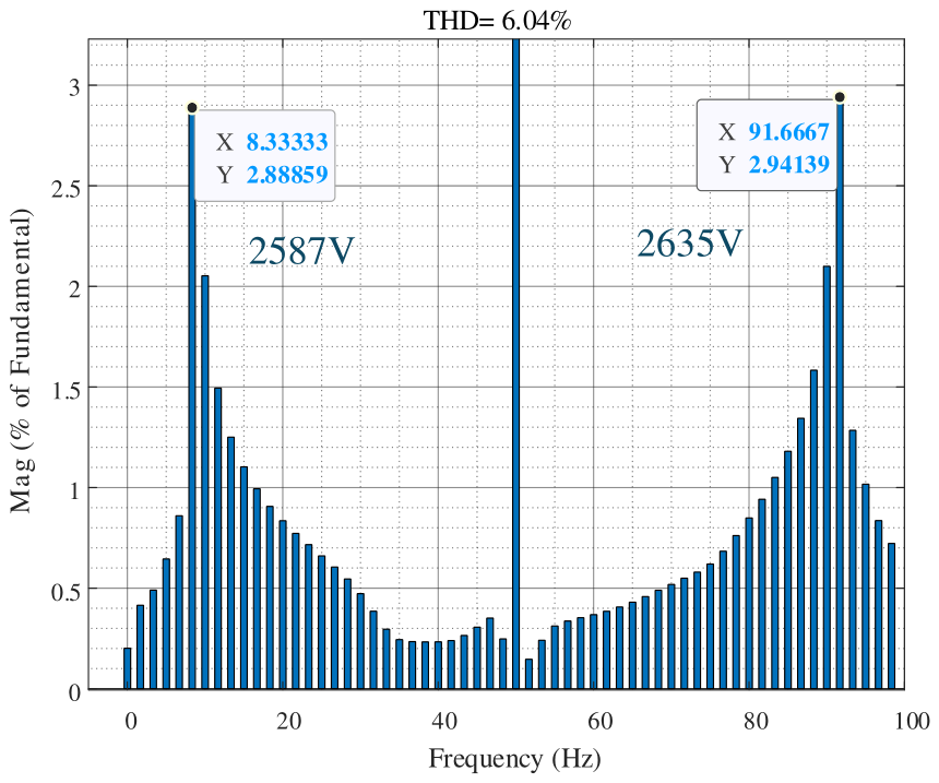
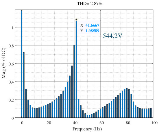
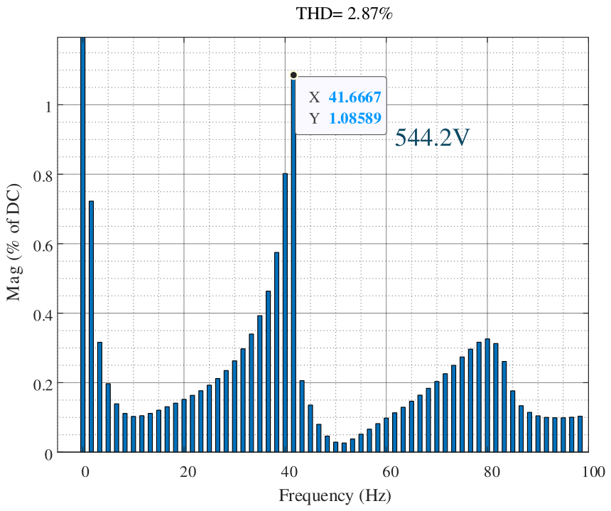
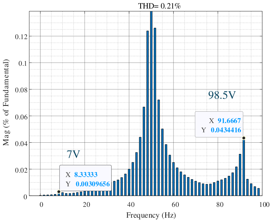
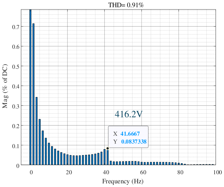
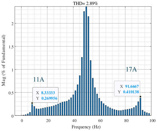
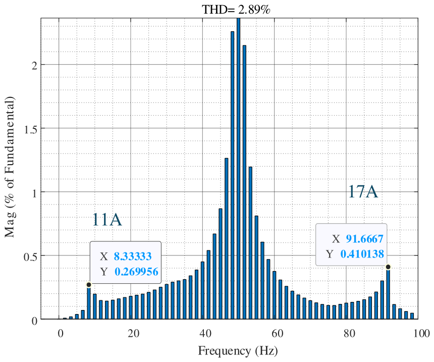
The wind-farm power is initially 0.4 p.u. and increases to 0.5 p.u. at approximately 7.0 s, as shown in Figure 6. The response develops an oscillation whose amplitude grows toward the end of the displayed interval. Figure 7, Figure 8, Figure 9, Figure 10, Figure 11, Figure 12 and Figure 13 show the associated terminal spectra. Because the response is nonstationary, spectral amplitudes depend on the selected observation window. The comparison below therefore assesses the frequency correspondence and reported attenuation trend without treating the spectra as a steady-state frequency-response measurement.

Figure 6. Wind-farm active-power response to the step from 0.4 to 0.5 p.u.

Figure 7. Fast Fourier transform (FFT) spectrum of the sending-end AC current, showing components at 8.3 and 91.7 Hz.

Figure 8. FFT of the sending-end hybrid-converter DC current; the translated component occurs at 41.7 Hz.

Figure 9. FFT of the sending-end hybrid-converter AC voltage.

Figure 10. FFT of the sending-end hybrid-converter DC voltage.

Figure 11. FFT of the receiving-end MMC AC voltage.

Figure 12. FFT of the receiving-end MMC DC voltage.

Figure 13. FFT of the receiving-end MMC AC current.

At the sending-end AC terminal, Figure 7 shows reported current components at 8.3 and 91.7 Hz, with annotated amplitudes of 274 A and 403 A, respectively. Figure 8 shows a reported DC-current component of 99.8 A at 41.7 Hz. These frequencies satisfy the mapping in Section 2.2 to the reported precision: 91.7 – 50 = 41.7 Hz and 100 − 91.7 = 8.3 Hz. Because the FFT spectra are normalized quantities and the corresponding amplitude bases are not explicitly used in the propagation-coefficient calculation, the annotated amplitudes are employed here for qualitative comparison. The reduced DC-current component is qualitatively consistent with the attenuating trend of the AC-to-DC current propagation coefficient at f_p = 91.7 Hz.

The 91.7 Hz component identified in the power-step response is used as the reference AC frequency for interpreting the associated 8.3 Hz AC and 41.7 Hz DC peaks, consistent with the frequency mapping in Section 2.2.

The voltage spectra exhibit the same frequency correspondence. Figure 9 contains AC-voltage components of 2587 V at 8.3 Hz and 2635 V at 91.7 Hz. Their similar magnitudes show that both components should be retained in the propagation assessment. The sending-end DC-voltage component at 41.7 Hz is 544.2 V in Figure 10. The attenuation trend at this frequency is consistent with the negative voltage coefficient at f_p = 91.7 Hz; the amplification peak near 50 Hz refers to a different part of the sweep.

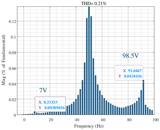
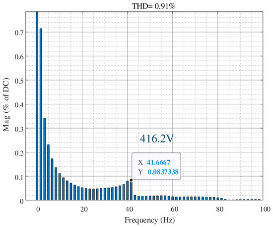
At the receiving end, the reported DC-voltage component is 416.2 V at 41.7 Hz in Figure 12. The AC-voltage components in Figure 11 are 7 V at 8.3 Hz and 98.5 V at 91.7 Hz, while the AC-current components in Figure 13 are 11 A and 17 A, respectively. These results support attenuation toward the receiving-end AC terminal in the investigated case. The sending- and receiving-end DC spectra both contain the translated 41.7 Hz component, confirming the propagation of the oscillatory component through the DC network.

The theoretical attenuation trend is obtained by solving the coupled terminal equations in (8) and evaluating the propagation coefficients in (9)–(14). A coefficient below unity, or below 0 dB, predicts attenuation under the stated amplitude normalization. At f_p = 91.7 Hz, Figure 2, Figure 3, Figure 4 and Figure 5 indicate attenuation at both converter stages. Using the RSS definition in Section 4, the reported FFT voltage amplitudes give sending-end AC-to-DC, DC-network, and receiving-end DC-to-AC ratios of 0.1474 (−16.63 dB), 0.7648 (−2.33 dB), and 0.2373 (−12.50 dB), respectively. Together with the 8.3/91.7 Hz AC and 41.7 Hz DC frequency correspondence, these results support the predicted attenuation trend.

The post-step response is nonstationary, so absolute FFT amplitudes depend on the position and duration of the observation window. For an isolated modal component with growth rate σ, shifting a fixed-duration rectangular window by Δt changes its exact-frequency amplitude estimate by the factor exp(σΔt). With identical synchronized windows and consistent normalization, the common envelope factor can cancel in terminal amplitude ratios, including RSS-based ratios, when one mode dominates and spectral interference is negligible. The spectra illustrate the AC/DC frequency correspondence and case-specific amplitude distribution; a numerical window-sensitivity bound requires comparison of synchronized time records over different windows.

5.4. Interpretation and Limitations

The framework complements an impedance-stability assessment. A generalized Nyquist or closed-loop modal calculation addresses the existence and growth of a mode, whereas the propagation coefficients describe its relative terminal responses under the specified boundary conditions. Compared with propagation analysis for MMC multi-terminal networks [26] and cascaded hybrid HVDC systems [27], the present application follows the DRU-MMC sending terminal and evaluates voltage and current separately. Its usefulness lies in connecting the measured AC and DC spectral components to the corresponding parts of the impedance model.

The oscillation source, propagation path, and largest-amplitude location describe different aspects of an oscillatory response. The source is the forcing mechanism or destabilizing interaction that generates or sustains the oscillation. The propagation path describes how the associated components are transferred among interconnected AC and DC terminals. The largest-amplitude location is the terminal at which a specified oscillatory voltage or current quantity exhibits its greatest amplitude. Terminal responses depend jointly on the excitation, converter dynamics, network transfer characteristics, and terminal impedances; consequently, a response maximum can occur at a location different from the source. Meaningful amplitude comparisons require consistent physical quantities, frequency mapping, and normalization conventions.

In the investigated case, the reported spectra and voltage–amplitude ratios characterize the coupled AC/DC response and indicate prominent oscillatory components at the offshore hybrid-converter AC terminal. These findings support considering this terminal as a monitoring location for the associated components. The physical mechanism responsible for the oscillation can be investigated through complementary stability or modal analysis [28].

The conclusions apply to the investigated parameter set, operating condition, and retained small-signal channels. Changes in grid strength, cable parameters, and controller settings modify the terminal impedances and DC-network response and may alter modal frequencies, growth rates, and amplitude ratios. Applying the propagation framework under these conditions requires updating the operating-point model and comparing its predictions with the corresponding time-domain responses. At fixed fundamental frequency, the frequency-mapping relations retain their form, while the numerical results remain case-specific. The series DC-network approximation excludes shunt-current redistribution, and the plotted band does not establish behavior outside 1–100 Hz. A single power-step case does not establish robustness to changes in grid strength, cable parameters, or controller settings. The method also does not describe saturation, protection action, severe faults, or changes in DRU conduction mode. Studies of wind-turbine operation under grid faults also address sensorless control of doubly fed induction generators with fault ride-through capability [31]. The nonstationary spectra illustrate the propagation pattern but do not provide an independent numerical calibration of the analytical coefficients. Further validation should use matched small-signal injections at several operating points, report magnitude and phase errors, and assess the effect of cable-model and harmonic-order choices before extending the conclusions to equipment stress or controller design.

The proposed framework is intended for small-signal oscillation-propagation analysis in DRU–MMC HVDC systems around a specified operating point. The investigated case illustrates the coupled AC/DC frequency components and the distribution of voltage and current oscillations across the converter terminals under the stated system and control parameters. Analysis at other operating conditions requires updating the operating-point model and the corresponding terminal impedances.

6. Conclusions

For the investigated 1000 MW DRU-MMC HVDC system, the impedance-based framework relates the 8.3 and 91.7 Hz AC components to the 41.7 Hz DC component following a power increase from 0.4 to 0.5 p.u., with reported voltage annotations yielding sending-end DC/AC root-sum-square (RSS), receiving-end AC-RSS/DC, and receiving/sending DC amplitude ratios of 0.1474 (−16.63 dB), 0.2373 (−12.50 dB), and 0.7648 (−2.33 dB), respectively, which quantify the voltage distribution in this case and support coordinated terminal monitoring but do not independently validate the analytical coefficients or identify the oscillation source without complementary stability or modal analysis.

References

- Li, Z.; Song, Q.; An, F.; Zhao, B.; Yu, Z.; Zeng, R. Review on DC transmission systems for integrating large-scale offshore wind farms. Energy Convers. Econ. 2021, 2, 1–14. [Google Scholar] [CrossRef] [Scilit]
- Yu, L.; Fu, Z.; Li, R.; Zhu, J. DRU-HVDC for offshore wind power transmission: A review. IET Renew. Power Gener. 2024, 18, 2080–2101. [Google Scholar] [CrossRef] [Scilit]
- Bidadfar, A.; Saborío-Romano, O.; Cutululis, N.A.; Sørensen, P.E. Control of offshore wind turbines connected to diode-rectifier-based HVDC systems. IEEE Trans. Sustain. Energy 2021, 12, 514–523. [Google Scholar] [CrossRef] [Scilit]
- Yu, L.; Li, R.; Xu, L. Distributed PLL-based control of offshore wind turbines connected with diode-rectifier-based HVDC systems. IEEE Trans. Power Deliv. 2018, 33, 1328–1336. [Google Scholar] [CrossRef] [Scilit]
- Zhang, Z.; Jin, Y.; Xu, Z. Grid-forming control of wind turbines for diode rectifie r unit based offshore wind farm integration. IEEE Trans. Power Deliv. 2023, 38, 1341–1352. [Google Scholar] [CrossRef] [Scilit]
- Chang, Y.R.; Cai, X. Hybrid topology of a diode-rectifier-based HVDC system for offshore wind farms. IEEE J. Emerg. Sel. Top. Power Electron. 2019, 7, 2116–2128. [Google Scholar] [CrossRef] [Scilit]
- Nguyen, T.H.; Lee, D.C.; Kim, C.K. A series-connected topology of a diode rectifier and a voltage-source converter for an HVDC transmission system. IEEE Trans. Power Electron. 2014, 29, 1579–1584. [Google Scholar] [CrossRef] [Scilit]
- Li, R.; Xu, L. A unidirectional hybrid HVDC transmission system based on diode rectifier and full-bridge MMC. IEEE J. Emerg. Sel. Top. Power Electron. 2021, 9, 6974–6984. [Google Scholar] [CrossRef] [Scilit]
- Xiao, H.Q.; Gan, H.C.; Dong, Y.Q.; Huang, Y.; Liu, Y.L. Control and capacity design of station-hybrid HVDC system with DRU and MMC in parallel for offshore wind power integration. IEEE Trans. Power Deliv. 2024, 39, 1783–1793. [Google Scholar] [CrossRef] [Scilit]
- Gan, H.C.; Xiao, H.Q.; Huang, Y.; Zhang, L.D. Cost-efficient hybrid converter for large-scale offshore wind power transmission. IEEE Trans. Power Deliv. 2025, 40, 1621–1633. [Google Scholar] [CrossRef] [Scilit]
- Wang, C.D.; Ali, A.; Blaabjerg, F. Composition and control of a new type of hybrid voltage-source converter based on DRUs and FB-MMC for large-scale offshore wind power integration and transmission. IEEE Trans. Power Electron. 2024, 39, 5721–5732. [Google Scholar] [CrossRef] [Scilit]
- Zhang, G.; Xiang, W.; Wen, J. Impedance modeling and stability analysis of DR-MMC based hybrid HVDC for offshore wind farm integration. IEEE Trans. Power Deliv. 2023, 38, 4397–4409. [Google Scholar] [CrossRef] [Scilit]
- Wu, W.; Wang, M.; Tu, L.; Cai, H.; Yan, G.; Qu, X.; Gu, H.; Chen, W. Control, modeling and stability analysis of DRU-based grid-forming converter. Chin. J. Electr. Eng. 2025, 11, 83–92. [Google Scholar] [CrossRef] [Scilit]
- Sun, J. Impedance-based stability criterion for grid-connected inverters. IEEE Trans. Power Electron. 2011, 26, 3075–3078. [Google Scholar] [CrossRef] [Scilit]
- Cespedes, M.; Sun, J. Impedance modeling and analysis of grid-connected voltage-source converters. IEEE Trans. Power Electron. 2014, 29, 1254–1261. [Google Scholar] [CrossRef] [Scilit]
- Rygg, A.; Molinas, M.; Zhang, C.; Cai, X. A modified sequence-domain impedance definition and its equivalence to the dq-domain impedance definition for the stability analysis of AC power electronic systems. IEEE J. Emerg. Sel. Top. Power Electron. 2016, 4, 1383–1396. [Google Scholar] [CrossRef] [Scilit]
- Wang, X.; Blaabjerg, F. Harmonic stability in power electronic-based power systems: Concept, modeling, and analysis. IEEE Trans. Smart Grid 2019, 10, 2858–2870. [Google Scholar] [CrossRef] [Scilit]
- Ji, K.; Tang, G.; Pang, H.; Yang, J. Impedance modeling and analysis of MMC-HVDC for offshore wind farm integration. IEEE Trans. Power Deliv. 2020, 35, 1488–1501. [Google Scholar] [CrossRef] [Scilit]
- Ji, K.; Pang, H.; Yang, J.; Tang, G. DC side harmonic resonance analysis of MMC-HVDC considering wind farm integration. IEEE Trans. Power Deliv. 2021, 36, 254–266. [Google Scholar] [CrossRef] [Scilit]
- Xue, T.; Lyu, J.; Wang, H.; Cai, X. A complete impedance model of a PMSG-based wind energy conversion system and its effect on the stability analysis of MMC-HVDC connected offshore wind farms. IEEE Trans. Energy Convers. 2021, 36, 3449–3461. [Google Scholar] [CrossRef] [Scilit]
- Xu, Z.; Li, B.; Han, L.; Hu, J.; Wang, S.; Zhang, S.; Xu, D. A complete HSS-based impedance model of MMC considering grid impedance coupling. IEEE Trans. Power Electron. 2020, 35, 12929–12948. [Google Scholar] [CrossRef] [Scilit]
- Lu, D.; Wang, X.; Blaabjerg, F. Impedance-based analysis of DC-link voltage dynamics in voltage-source converters. IEEE Trans. Power Electron. 2019, 34, 3973–3985. [Google Scholar] [CrossRef] [Scilit]
- Zhang, C.; Cai, X.; Molinas, M.; Rygg, A. On the impedance modeling and equivalence of AC/DC-side stability analysis of a grid-tied type-IV wind turbine system. IEEE Trans. Energy Convers. 2019, 34, 1000–1009. [Google Scholar] [CrossRef] [Scilit]
- Pedra, J.; Sainz, L.; Monjo, L. Three-port small-signal admittance-based model of VSCs for studies of multi-terminal HVDC hybrid AC/DC transmission grids. IEEE Trans. Power Syst. 2021, 36, 732–743. [Google Scholar] [CrossRef] [Scilit]
- Zhao, C.; Jiang, Q. Impedance-based AC/DC terminal modeling and analysis of the MMC-BTB system. IEEE Trans. Power Deliv. 2024, 39, 542–554. [Google Scholar] [CrossRef] [Scilit]
- Cao, Y.; Du, X.; Liu, J.; Tai, H.M.; Du, C.; Zou, X. Characterizing sub-synchronous oscillation propagation in MMC-MTDC system based on SSO propagation coefficients. IEEE Trans. Power Syst. 2024, 39, 7025–7037. [Google Scholar] [CrossRef] [Scilit]
- Xu, R.; Jiang, Q.; Li, B.; Liu, Y.; Liu, T.; Blaabjerg, F.; Wang, P. Impedance based stability analysis of the multi-terminal cascaded hybrid HVDC system. IEEE Trans. Power Deliv. 2025, 40, 1754–1768. [Google Scholar] [CrossRef] [Scilit]
- Zhang, Z.; Kou, P.; Mei, M.; Tian, R.; Zhang, Y.; Liang, D. Interaction analysis and damping control of sub-synchronous oscillation and medium-frequency oscillation in HVDC-connected offshore wind farm. IEEE Trans. Power Syst. 2025, 40, 4336–4352. [Google Scholar] [CrossRef] [Scilit]
- Huang, X.; Hu, B.; Zhang, S.; Lu, K.; Chen, Z.; Li, H. Interaction Impact and Coordinated Mitigation Strategy of Low Frequency Oscillations with Torsional Vibrations for GFM-DFIG Wind Turbine. IEEE Trans. Ind. Appl. 2026; early access. [CrossRef] [Scilit]
- Zhu, X.; Zhang, H.; Ren, H.; Huang, P.; Wang, Y.; Cao, D. Energy Storage Units Optimal Operation Strategy With Efficiency Improvement and State of Charge Balance. IEEE Trans. Ind. Appl. 2026; early access. [CrossRef] [Scilit]
- Zeng, W.; Wang, T.; Wang, Y.; Wu, H.; Meng, X.; Zhao, C.; Zhang, Z.; Wu, L. Sensorless control of doubly-fed induction generators with grid fault ride-through capability. IEEE Trans. Energy Convers. 2026; early access. [CrossRef] [Scilit]
Disclaimer/Publisher’s Note: The statements, opinions and data contained in all publications are solely those of the individual author(s) and contributor(s) and not of MDPI and/or the editor(s). MDPI and/or the editor(s) disclaim responsibility for any injury to people or property resulting from any ideas, methods, instructions or products referred to in the content. |
© 2026 by the authors. Licensee MDPI, Basel, Switzerland. This article is an open access article distributed under the terms and conditions of the Creative Commons Attribution (CC BY) license.