


Abstract
The interlayer is a key geological factor that regulates reservoir heterogeneity and remaining oil distribution, and its accurate identification directly affects the reservoir development effect. To address the strong subjectivity of traditional identification methods and the insufficient recognition accuracy of single machine learning models under imbalanced sample distributions, this study focuses on three types of interlayers (argillaceous, calcareous, and petrophysical interlayers) in the W Oilfield, and proposes an accurate identification method integrating the Synthetic Minority Over-Sampling Technique (SMOTE) and heterogeneous ensemble learning. Firstly, the corresponding data set of interlayer type and logging response is established. After eliminating the influence of dimension using normalization, the sensitive logging curves are optimized using the crossplot method, mutual information, and effect analysis. SMOTE technology is used to balance the sample distribution and solve the problem of the identification deviation of minority interlayers. Then, a heterogeneous ensemble model composed of the k-nearest neighbor algorithm (KNN), decision tree (DT), and support vector machine (SVM) is constructed, and the final recognition result is output using a voting strategy. The experiments show that SMOTE technology improves the average accuracy of a single model by 3.9% and effectively improves the model bias caused by sample imbalance. The heterogeneous integration model improves the overall recognition accuracy to 92.6%, significantly enhances the ability to distinguish argillaceous and petrophysical interlayers, and optimizes the F1-Score simultaneously. This method features a high accuracy and reliable performance, providing robust support for interlayer identification in reservoir geological modeling and remaining oil potential tapping, and demonstrating prominent practical application value.
1. Introduction
Interlayers, as critical geological barriers regulating reservoir heterogeneity and remaining oil distribution, directly determine the efficiency of reservoir development and remaining oil tapping [1,2]. The accurate identification of interlayer types and spatial distribution is therefore essential for reservoir numerical simulation, development plan optimization, and enhanced oil recovery. The core description method, while intuitive and accurate, is limited by high coring costs and sparse coring wells, making large-scale application in oilfields impractical [3]. Logging data, as a comprehensive reflection of formation physical properties, provides a cost-effective alternative for interlayer identification, as different interlayer types exhibit distinct logging response characteristics that can be calibrated via core data. Based on the core calibration, the corresponding relationship between different types of interlayers and logging response characteristics can be established, so as to establish the identification standard of interlayers to identify interlayers in uncored wells. Because the logging data is easy to obtain, this method is widely used in identifying the interlayer. At present, commonly used interlayer identification methods based on logging data mainly fall into two categories: (1) Direct identification methods based on logging curves or cut-off values of reservoir parameters [4,5]. Although the direct method is simple, it only uses the cut-off value for identification, and the judgment process involves subjectivity, resulting in the lack of a unified identification standard. (2) Graphical methods such as crossplot [6,7,8,9], ternary diagram [10], and cobweb diagram methods [11,12,13], which are based on the sensitivity analysis of logging curves and reservoir parameters. The crossplot method is the most widely used technique for interlayer identification. It involves selecting logging curves sensitive to interlayers, plotting crossplots through pairwise combinations, and establishing identification criteria for different types of interlayers, which has achieved favorable results. However, the logging response characteristics of argillaceous interlayers and petrophysical interlayers are often minimally distinguishable, leading to an unsatisfactory identification performance using two-dimensional sensitive logging curves. The cobweb diagram can make full use of multiple logging curves to identify the types of interlayers according to the morphological differences in different interlayers. In fact, it reflects the differences in logging response characteristics of different interlayers. Although the cobweb diagram method is more intuitive in identifying interlayers, it is less amenable to programming. Different from the above methods, in recent years, an increasing number of scholars have applied machine learning (ML) to solve regression problems (reservoir parameter calculation and curve reconstruction, etc.) and classification problems (fluid identification, lithology identification, reservoir classification, etc.) in logging interpretation. The identification of interlayer type is essentially a classification problem. Wang et al. used the calculated shale content, porosity, permeability, deep resistivity, and median grain size to identify the interlayer using gray relation analysis (GRA) [14]. Qu et al. combined conventional logging curves with calculated porosity and permeability, and introduced a wavelet neural network for interlayer identification, achieving a favorable recognition performance [15]. Yi et al. used the crossplot method to select natural gamma, acoustic time difference, and resistivity as the main sensitive parameters, used the gray relation analysis to calculate the weight coefficient, and obtained the comprehensive discriminant index to quantitatively identify the interlayer [16]. He used SVM to advance the characterization of interlayers to quantitatively identify interlayer types using evaluation parameters such as natural gamma ray (GR), acoustic time difference (AC), and micro electrodes to improve the accuracy of interlayer type identification [17]. Chen used GR, AC, neutron (CNL), density (DEN), and porosity (POR) as input parameters, and used the support vector machine method on the basis of principal component analysis [18]. Chen et al. proposed an ensemble auto encoder algorithm based on semi-supervised collaborative training for the actual situation of less coring logging data and unbalanced samples [19]. Zheng used an image of a logging curve to identify the interlayer in a reservoir based on a convolutional neural network, but this method involves converting the logging data into a logging image and performing a series of processing steps on the image [20]. However, existing machine learning-based approaches face three key limitations in interlayer identification: (1) the inadequate handling of imbalanced sample distributions; interlayers are spatially discrete, leading to “majority dominance and minority scarcity”, resulting in biased overfitting to majority classes; (2) the limited accuracy of single models due to algorithmic constraints; (3) a lack of systematic feature selection strategies, with the arbitrary selection of logging curves leading to redundant information and reduced model interpretability. Thus, this study develops an approach integrating SMOTE and heterogeneous ensemble learning to classify interlayer types (calcareous, argillaceous, and petrophysical) in the W Oilfield. The framework synchronously ensures feature informativeness and category discriminability by screening sensitive logging curves via mutual information and effect size, laying a high-quality data foundation for subsequent modeling. Considering sample imbalance in three interlayer types in the W Oilfield, SMOTE is adopted to supplement minority samples, while a heterogeneous ensemble model is constructed using complementary base learners (KNN, DT, and SVM). This integration achieves an overall interlayer identification accuracy of 92.6% and significantly improves the distinguishability between argillaceous and petrophysical interlayers. This integration attempts to address the challenges of traditional methods and single ML models in interlayer identification, with a focus on practicality and extensibility rather than developing novel algorithms. It provides a reliable geological basis for the fine characterization of interlayers and the potential tapping of remaining oil in reservoir numerical simulation, and has important practical significance for improving oilfield development efficiency.
2. Method
2.1. Imbalanced Data Sets and SMOTE Algorithm
Imbalanced data sets refer to the significant differences in the number of samples of different categories [21,22]. SMOTE has been widely adopted by numerous scholars to address the imbalanced data problem in geoscience-related classification tasks (e.g., lithology identification, reservoir parameter prediction) [23,24,25,26,27]. Its core idea is based on the feature space distribution of minority class samples. By calculating the feature difference between the minority class samples and their neighboring samples, the new synthetic samples are generated by linear interpolation, which not only does not change the feature law of the original samples, but also can supplement the number of minority class samples. The specific operation is that for each sample in the minority class, -nearest neighbor samples are obtained by calculating the Euclidean distance between it and all minority class samples. For each minority class sample, a sample in its k-nearest neighbor is randomly selected and a new composite sample is generated between them. The specific formula is as follows:
where denotes the newly generated synthetic sample; is the target sample from the minority class; is a randomly selected sample from the k-nearest neighbors of ; and is a random number within the interval (0, 1), which controls the position of between and .
The generated new samples are added to the original data set, so that the number of samples in each interlayer category in the data set is more balanced. The above steps are repeated many times until the number of samples in each minority class is balanced.
2.2. Ensemble Learning
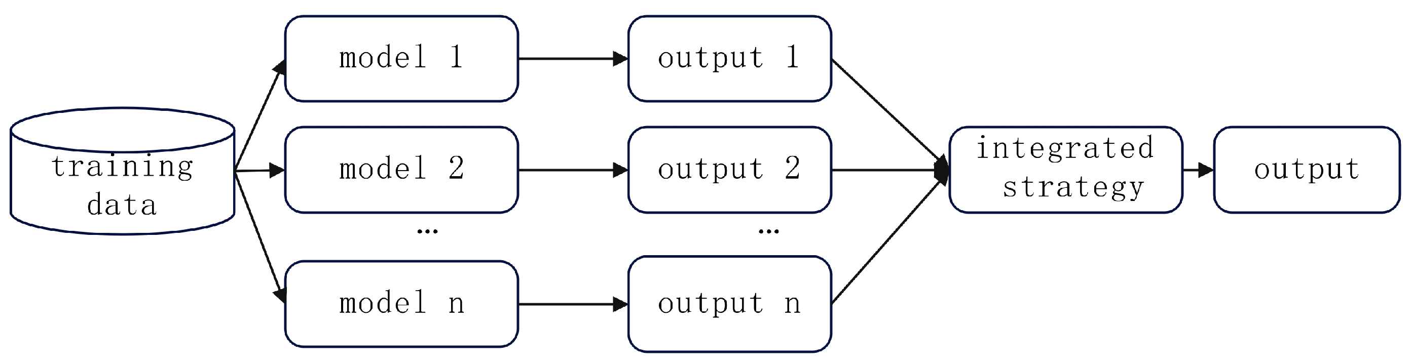
In view of the limitations faced by current single intelligent algorithms in geophysical logging interpretation, ensemble learning is a more suitable and flexible solution [28,29]. It integrates multiple single machine learning models through a specific strategy to form a robust model, thereby improving prediction accuracy. Its general structure is shown in Figure 1.
Figure 1.
Schematic diagram of ensemble learning.
Homogeneous integration and heterogeneous integration are the two main integration methods in ensemble learning. In homogeneous ensembles, all individual learners are combined by the same base learner. In heterogeneous ensembles, different types of individual learners are combined. This method can obtain a better generalization ability by the difference between different learners. Tan et al. and Bai Yang et al. used a committee machine in ensemble learning for fluid identification [30,31] and organic carbon content prediction [32], and achieved favorable results. Aiming at the problem of interlayer recognition, the heterogeneous ensemble learning method combined with the voting strategy of a majority vote is used to select the interlayer recognition results, so that even if some learners have errors, they can be corrected by majority learners.
2.3. The Interlayer Identification Process Based on SMOTE and Ensemble Learning
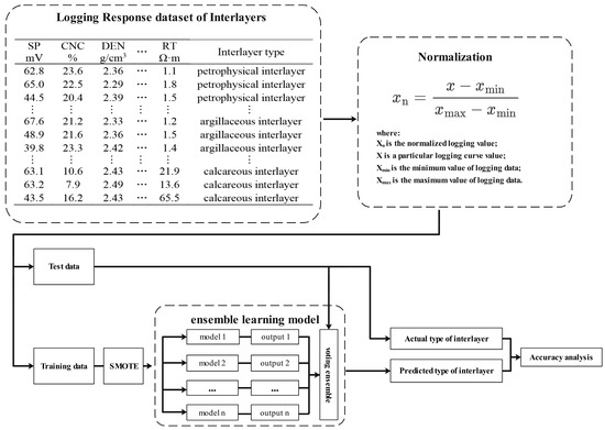
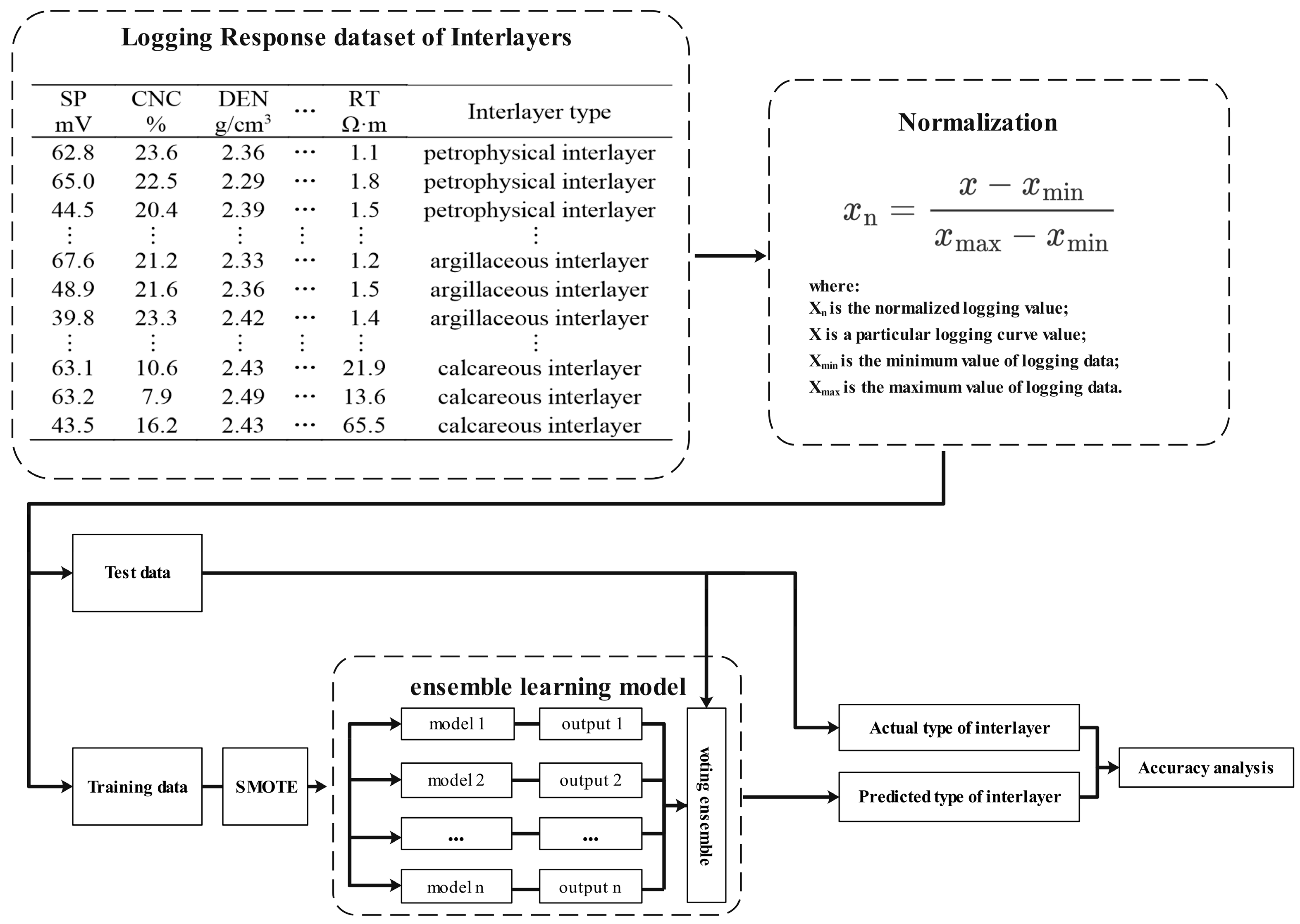
Imbalanced data sets have a negative impact on the performance of machine learning algorithms. In the training process, the algorithm will learn more features of a large number of categories, while ignoring the features of a small number of categories. This may lead to a decrease in the accuracy of the algorithm because it cannot correctly identify a small number of categories. The proposed interlayer identification workflow integrates data preprocessing, model training, and performance verification, with core components designed to address unbalanced data and improve recognition accuracy (Figure 2). First, a logging response data set for interlayers in the study area is established via core-calibrated logging data. Next, normalization is applied to eliminate numerical and dimensional discrepancies among logging curves, enhancing the model’s ability to capture spatial correlations between inputs and outputs. The normalized dataset is randomly split into a training set (80%) and test set (20%)—a ratio balancing sufficient feature learning and objective generalization verification. Minority interlayer samples in the training set are balanced using SMOTE to mitigate bias from class imbalance, and a heterogeneous ensemble model is constructed with KNN, DT, and SVM as base learners. The final recognition results are generated via a majority voting strategy to leverage the complementary strengths of each algorithm.
Figure 2.
Flow chart of interlayer identification based on SMOTE and ensemble learning.
3. Application Examples and Analysis
3.1. Data Establishment
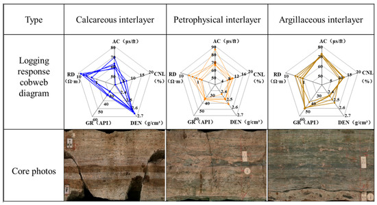
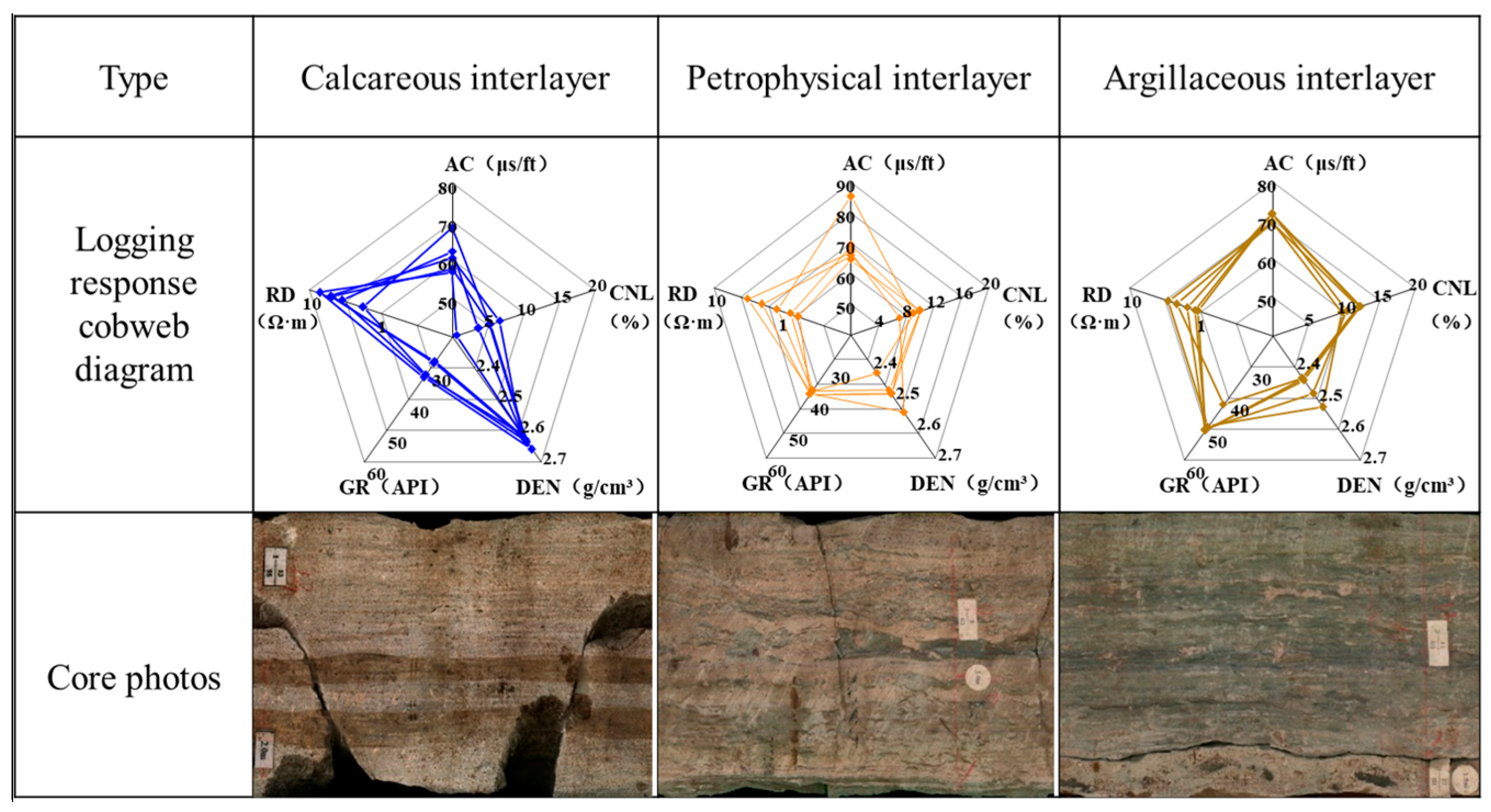
In this paper, the logging curve of the experimental well in the W Oilfield is selected as the data basis. The W Oilfield is a bottom water reservoir, and the distribution of remaining oil is complex. Most of the production wells are at the middle and high water cut stage, and there is a risk of water flooding on the plane. The distribution form of the interlayer has a great influence on the evaluation results of logging reservoir parameters. It is urgent to carry out research on the fine identification technology of the interlayer in the study area, so as to provide effective technical support for the accurate characterization of the remaining oil distribution in the W Oilfield and lay an important foundation for the adjustment of oilfield production and the development plan. The target layer of the oilfield has argillaceous, calcareous, and petrophysical interlayers, among which the calcareous interlayers are widely developed. For the calcareous interlayer, the lithological characteristics are mainly calcium-bearing fine sandstone, calcareous fine sandstone, calcareous powder-fine sandstone, etc., and the logging characteristics are mainly a low gamma, low acoustic transit time, high density, low neutron, and high resistivity. For the petrophysical interlayer, the lithological characteristics are mainly calcium-containing argillaceous siltstone–fine sandstone, mud-containing calcareous siltstone–fine sandstone, and calcium-containing argillaceous siltstone. The logging characteristics are mainly a medium gamma, medium–high acoustic wave, high density, medium–high neutron, and medium–high resistivity. For the argillaceous interlayer, the lithologic characteristics are mainly argillaceous siltstone, argillaceous siltstone–fine sandstone, argillaceous fine sandstone, argillaceous fine sandstone, argillaceous fine sandstone, argillaceous siltstone–fine sandstone, silty mudstone, etc., and there are very few pure mudstone layers. The logging characteristics are mainly a medium–high gamma, high acoustic wave, high density, high neutron, and low resistivity (Figure 3).
Figure 3.
Core photos and logging response cobweb diagram of different types of interlayers.
On the basis of core calibration logging, this paper establishes the logging response characteristic data sets corresponding to different types of interlayers (Table 1). The data sets are collected from 14 wells in the W Oilfield (130 total samples: 55 calcareous, 41 argillaceous, 34 petrophysical). The logging curves in the original data set include natural gamma ray (GR), spontaneous potential (SP), well caliper (CAL), acoustic time difference (AC), density (DEN), neutron (CNL), deep resistivity (RD), shallow resistivity (RS), and flushed zone resistivity (RXO). Different interlayers have obvious differences in curve characteristics.
Table 1.
Logging response characteristic dataset of interlayers (partial).
3.2. Data Normalization
As a method of data standardization, data normalization plays an important role in data mining to eliminate the influence of dimension and range between different variables, improving the ability of machine learning methods to find the spatial relationship between input and output. From Table 1, we know that different types of logging data are quite different and have different dimensions. If these logging data are not processed and are used directly for training, it will result in slow model convergence and a low prediction accuracy. Based on the above questions, we have to normalize the obtained original interlayer logging response data set. For different types of logging data, it is necessary to select a suitable normalization method to eliminate the dimensional difference and ensure the validity of the data. In this paper, Min-Max normalization is utilized. It can completely retain the relative size relationship of the original data, which is highly consistent with the core target of identifying interlayers based on the difference in logging response. Compared with other normalization methods, the calculation logic is simple and the physical meaning is clear, which is convenient for the geological interpretation and verification of the subsequent results. It not only ensures the scientificity of data processing, but also provides reliable feature input for the accurate identification of interlayers.
For conventional logging curves such as GR, AC, DEN, and CNL, the numerical distribution is concentrated and there are no extreme outliers. The normalization can compress it to the range of [0, 1] and completely retain the relative distribution relationship of the original data, and does not change the response difference law between the curves. The formula is as follows:
where is any of the above logging data that needs to be normalized, is the corresponding logging data minimum value, is the corresponding logging data maximum value, and is the normalized logging data.
Due to the influence of reservoir fluid properties and lithologic changes, the resistivity logging curve has a very wide range in terms of it numerical distribution. The logarithm is first transformed into an approximate normal distribution and then the values are normalized, which can effectively suppress the interference of extreme values on the normalization results, while retaining its sensitive characteristics to lithologic changes.
where is the normalized resistivity logging data, is the resistivity logging curve, is the minimum value of the resistivity logging data, is the maximum value of the resistivity logging data, and lg indicates the common logarithm with a base of 10, ensuring consistency in logarithmic calculation standards. RD, RS, and RXO can be nomorlized using Formula (3).
3.3. Feature Selection
Feature selection refers to screening out a small part of the most discriminative logging curves from the original logging data, eliminating irrelevant or redundant feature curves to reduce the number of features, suppress noise overfitting, and achieve the purpose of reducing running time. Using multiple logging curves to identify interlayers, although the abundance of information is increased, irrelevant information will make the learning effect worse and introduce new errors. Therefore, feature selection is required before establishing a machine learning model. In the process of interlayer logging interpretation, it is necessary to analyze the sensitivity of logging curves to determine the relationship between the response of logging curves and the type of interlayer. This helps people to select more sensitive logging curves in interlayer identification and improve the accuracy of interlayer identification. The sensitivity analysis of logging curves plays a vital role in the identification of interlayers.
In order to quantitatively screen the logging features sensitive to the type of interlayer, this study uses mutual information (MI) and effect size (η2) as the indicators. Mutual information is used to measure the degree of information correlation between features and interlayer categories. The larger the value is, the stronger the interpretation ability of features to category labels is. The calculation formula is based on the definition of probability distribution (Formula (4)).
where is a single logging feature (such as GR, DT, etc.); is the interlayer category label (argillaceous interlayer, calcareous interlayer, petrophysical interlayer); and are the marginal probabilities of feature and category , respectively; and is the joint probability of feature and category .
The effect is used to quantify the ability of the feature to distinguish the difference between the interlayer categories. The larger the value, the more significant the difference between the different categories. The core of this effect is derived via analysis of variance (ANOVA) and can be calculated using Formulas (5)–(9).
where represents the original value of the logging feature for the i-th sample in the c-th interlayer category, is the sample size of the c-th interlayer category, is the mean value of the feature for the c-th interlayer category, is the sum of squares between groups, is the total sum of squares, is the total number of interlayer categories ( in this study), is the grand mean value of the feature, and is the total number of samples across all interlayer categories.
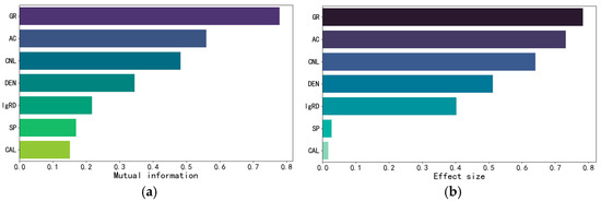
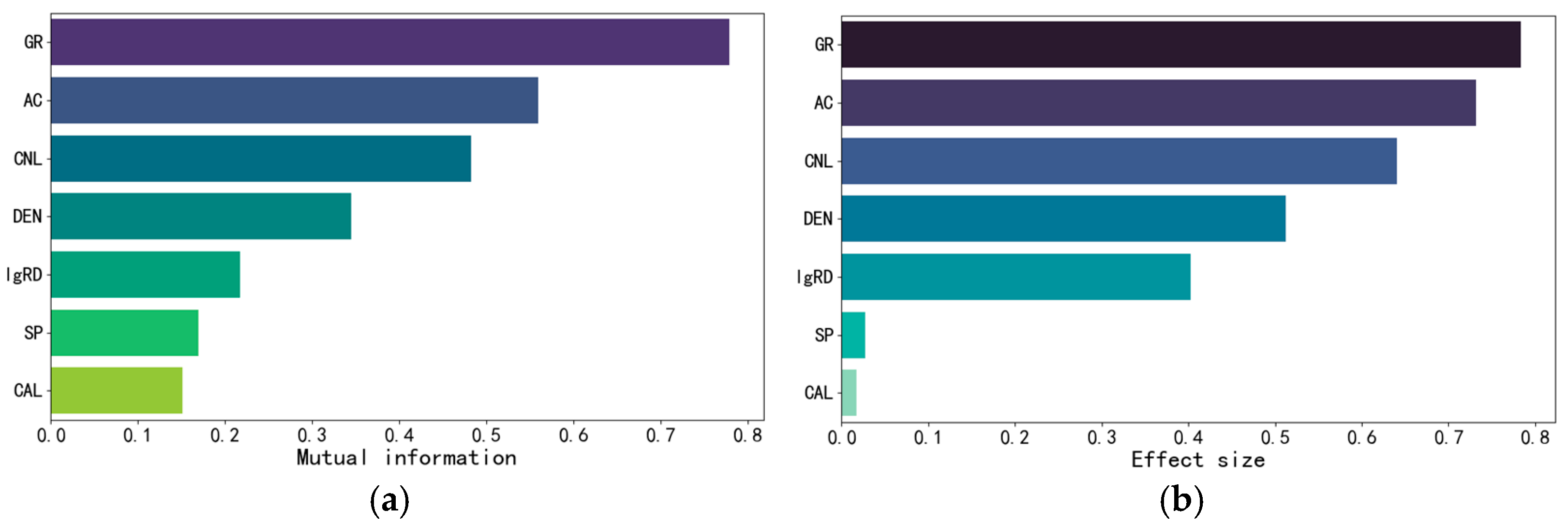
The simultaneous consideration of mutual information and effect size values enables the preferential selection of features that perform prominently in both indicators. This ensures the selected features are not only information-rich but also exert significant effects on category discrimination, thereby enhancing the model’s discriminative ability and interpretability. To clarify, the threshold in this study was derived from data-driven inflection point analysis (Figure 4). For effect size (η2), a dramatic drop in the η2 values of spontaneous potential (SP) and caliper (CAL) is observed beyond the inflection point at approximately η2 = 0.4, indicating a substantial decline in their explanatory power for the target interlayer classes. For mutual information (MI), the values of SP and CAL also present a distinct inflection point near MI = 0.2, beyond which the incremental gain in information related to the target variable plateaus. Therefore, GR, AC, CNL, DEN, and RD are ultimately selected as the input curves for interlayer type identification.
Figure 4.
Distributions of mutual information (MI) and effect size (η2) for logging curves. (a) MI distribution; (b) η2 distribution.
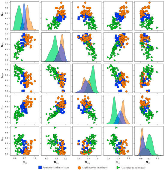
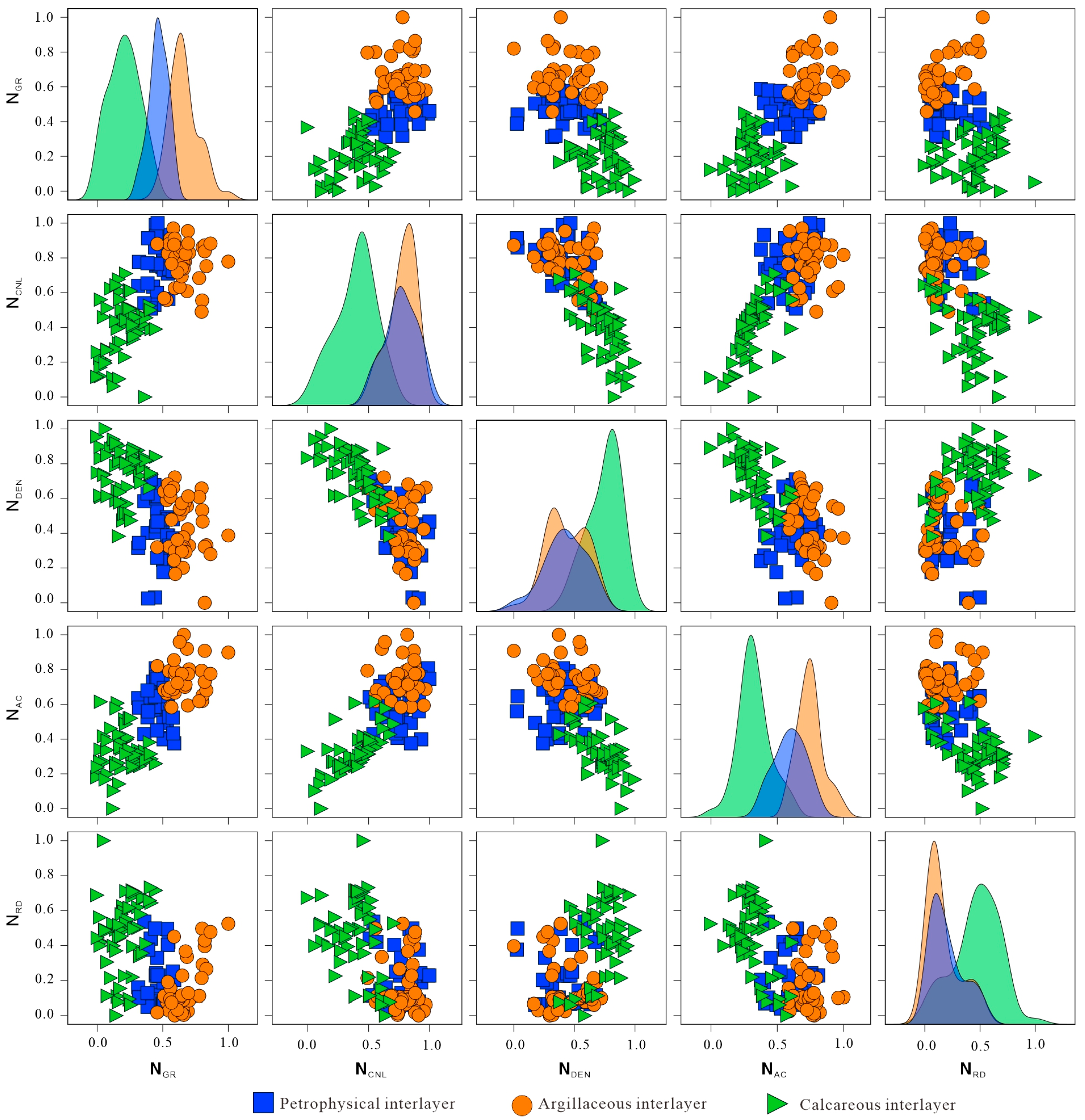
The crossplot of the selected characteristic curves is drawn to further analyze the logging response characteristics and optimization effects of different types of interlayers (Figure 5). It can be seen from Figure 5 that the data distribution of calcareous interlayers is obviously different from that of the other two types of interlayers, while the data points of argillaceous interlayers and petrophysical interlayers have no obvious boundary on the intersection chart. This is because petrophysical interlayers often contain shale, leading to similar logging response characteristics to argillaceous interlayers [33]. This similarity highlights the inherent limitation of traditional two-dimensional crossplots: they only utilize the linear correlation of two feature sets, failing to capture the complex nonlinear relationships among multiple features and thus struggling to distinguish categories with similar characteristics. The heterogeneous ensemble learning model adopted in this paper can break through this limitation. It integrates multiple sets of sensitive logging features and automatically mines the high-order correlations and nonlinear mapping rules between features. It can accurately capture the subtle difference characteristics of argillaceous and petrophysical interlayers. This effectively overcomes the defect of two-dimensional crossplots, and finally realizes the accurate identification of the three types of interlayers.
Figure 5.
Analysis of interlayer types and logging response characteristics.
3.4. Analysis of Interlayer Identification Results
The classification of interlayer type is a small sample classification problem. Due to the small number of data samples, some machine learning methods with good robustness to data need to be used. In order to build a heterogeneous ensemble model with an excellent performance, this paper chooses KNN, DT, and SVM as the base learners, and the core is based on the complementarity of the algorithm characteristics of the three. KNN realizes classification using feature similarity between samples, which is sensitive to local data features, can capture the subtle response differences in logging curves, and adapt to the local distribution law of interlayer characteristics. DT is good at mining the nonlinear correlation between features. The model structure is intuitive and interpretable. It can clearly reflect the logical relationship between logging features and interlayer categories, and has certain robustness to outliers. SVM transforms low-dimensional logging features into high-dimensional space through kernel function mapping, which can effectively deal with classification problems under high-dimensional data, and has excellent adaptability to scenes with more feature dimensions and blurred boundaries such as interlayers. The principles and advantages of the three algorithms complement each other, avoiding the limitations of a single model. The voting strategy is used to integrate the prediction results of each model to improve the overall recognition accuracy. All base learners are implemented based on the Python (version 3.11) scikit-learn library. The specific parameters are shown in Table 2.
Table 2.
Hyperparameters of different base learner models.
In machine learning classification problems, the indicators that measure the performance of the model generally include accuracy, recall, precision, and F1-Score. This paper selects accuracy and F1-Score as the core evaluation criteria to better evaluate the actual effect of the model. Among them, accuracy is one of the basic indicators of classifier performance, and it is also a commonly used evaluation criterion for classification problems in logging. It is used to measure the proportion of samples correctly classified by the classifier to the total number of samples. The calculation logic is the ratio of the number of correctly classified samples to the total number of samples, which can directly reflect the overall accuracy of the model classification results (Formula (10)).
where is the total number of categories; in this case = 3; represents the number of samples that are actually class i and predicted to be i.
Accuracy rate only reflects the overall performance of the classifier on the data set. Since the accuracy rate only measures the total number of correct classifications of the model, it cannot effectively evaluate the data set of unbalanced categories. Even if the classifier performs poorly in a few categories, it can obtain a high accuracy.
F1-Score is the harmonic average of precision and recall rate, so it can describe the advantages and disadvantages of the model more comprehensively than a single accuracy rate. As a general scale for binary classification, the range of F1-Score is 0~1, and the closer the value is to 1, the better the classification performance. Since the three types of interlayers have the same attention, the macro-average method is used to calculate the F1-Score of the multi-classification problem, so as to better evaluate the classification performance of the model. The specific calculation method is as follows:
- (1)
- Calculate the precision rate and recall rate of each category.
- (2)
- Calculate F1-Score for each category.
- (3)
- Calculate the average value of F1-Score for all categories.
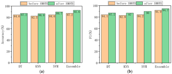
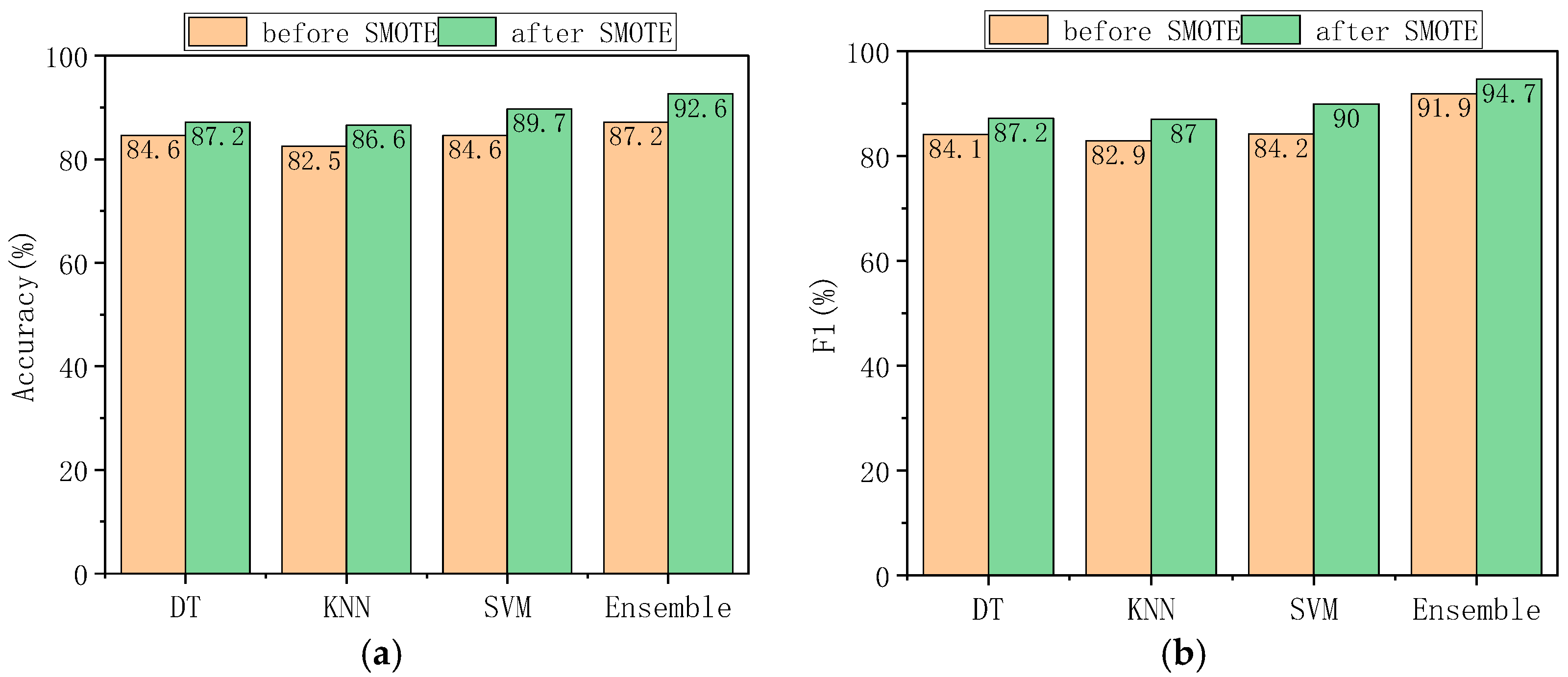
Firstly, the accuracy and overall performance of the three base models and heterogeneous integration models are evaluated. The accuracy and F1-Score of each model on the test set before and after data balance are shown in Figure 6. By comparing the prediction accuracy of the interlayer before and after the balance of the data set, it can be seen that after the data set is balanced by SMOTE, the prediction accuracy of the model is improved to varying degrees, among which KNN is increased by 4.1%, decision tree is increased by 2.6%, support vector machine is increased by 5.1%, and the accuracy of the three methods after voting integration is increased by 5.4%. After SMOTE processing, we compared the interlayer prediction accuracy of single machine learning models and the integrated model. The integrated model achieved a higher recognition accuracy, reaching 92.6%. This accuracy outperforms that of single machine learning models. The F1-Score increases synchronously, and the robustness of the overall prediction is significantly enhanced.
Figure 6.
Comparison of interlayer identification performance of different machine learning methods: (a) accuracy of each model before and after SMOTE data balancing; (b) F1-Score of each model before and after SMOTE data balancing (note: DT = decision tree, KNN = k-nearest neighbor, SVM = support vector machine, Ensemble = heterogeneous ensemble model).
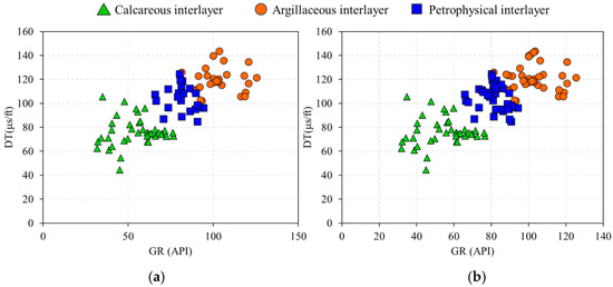
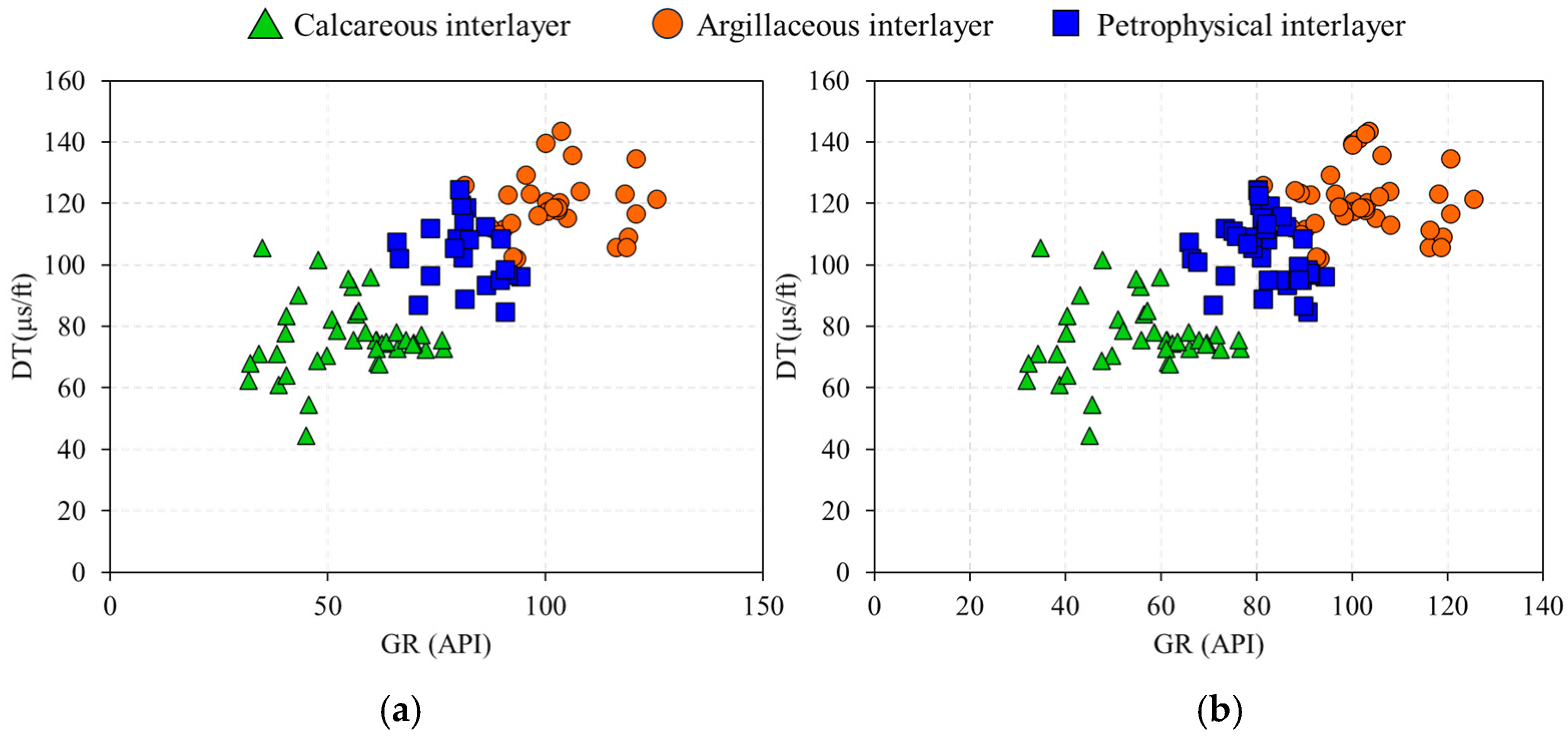
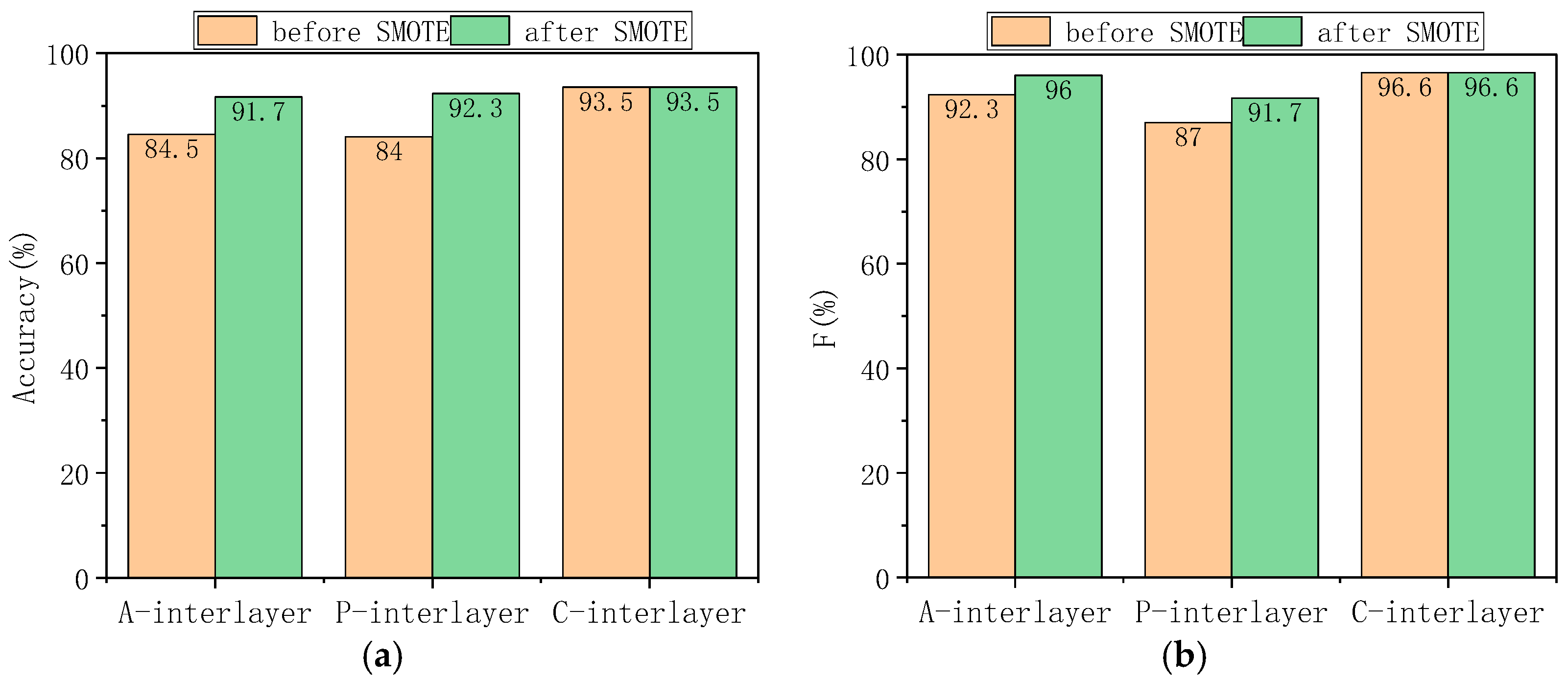
In order to study the prediction effect of SMOTE and the integrated model on different types of interlayers, taking GR-DT two-dimensional feature space as an example, the scatter plot of sample distribution before and after SMOTE treatment is drawn to visually display the change in sample distribution (Figure 7). SMOTE sampling ratios are determined to balance class distribution, resulting in 55 samples per class after processing. The effect of SMOTE can be clearly observed in Figure 7. Before treatment, the petrophysical interlayer samples and argillaceous interlayer samples are discretely distributed in the feature space, and there are feature blanks in some areas. After interpolation using SMOTE technology, the new samples are closely distributed in the feature-intensive areas of the original minority samples, and do not exceed the feature value range of the real samples, so as to ensure that the synthetic samples can truly reflect the geological characteristics of the interlayer and do not introduce false information. At the same time, the histogram of the accuracy rate and F1 before and after SMOTE was drawn according to the interlayer category (Figure 8). When SMOTE is not used, the accuracy and F1 value of most interlayers are generally at a high level due to the advantage of the number of samples, and the model can identify the characteristics of such interlayers more stably. However, due to the low proportion of samples and sparse data distribution, it is difficult for the model to fully capture its key information in the learning process, resulting in a significantly lower accuracy and F1 value. When the SMOTE algorithm is introduced for processing, the performance difference between these categories is significantly reduced. The accuracy of a few types of interlayers has been greatly improved: the accuracy of the original petrophysical interlayer with an accuracy of 84.0% has increased to 92.3% after SMOTE processing, and the accuracy of argillaceous interlayer recognition has increased from 84.5% to 91.7%. At the same time, the F1-Score also showed a trend of synchronous growth.
Figure 7.
Scatter plots of sample distribution in GR-DT two-dimensional feature space before and after SMOTE processing: (a) sample distribution before SMOTE processing (55 calcareous, 41 argillaceous, 34 petrophysical); (b) sample distribution after SMOTE processing (55 samples for each interlayer type).
Figure 8.
Comparison of performance for different interlayer types before and after SMOTE processing. (a) Accuracy of different interlayer types before and after SMOTE processing; (b) F1-Score of different interlayer types before and after SMOTE processing (note: A-interlayer = Argillaceous interlayer, P-interlayer = Petrophysical interlayer, C-interlayer = Calcareous interlayer).
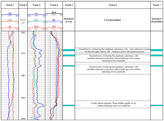
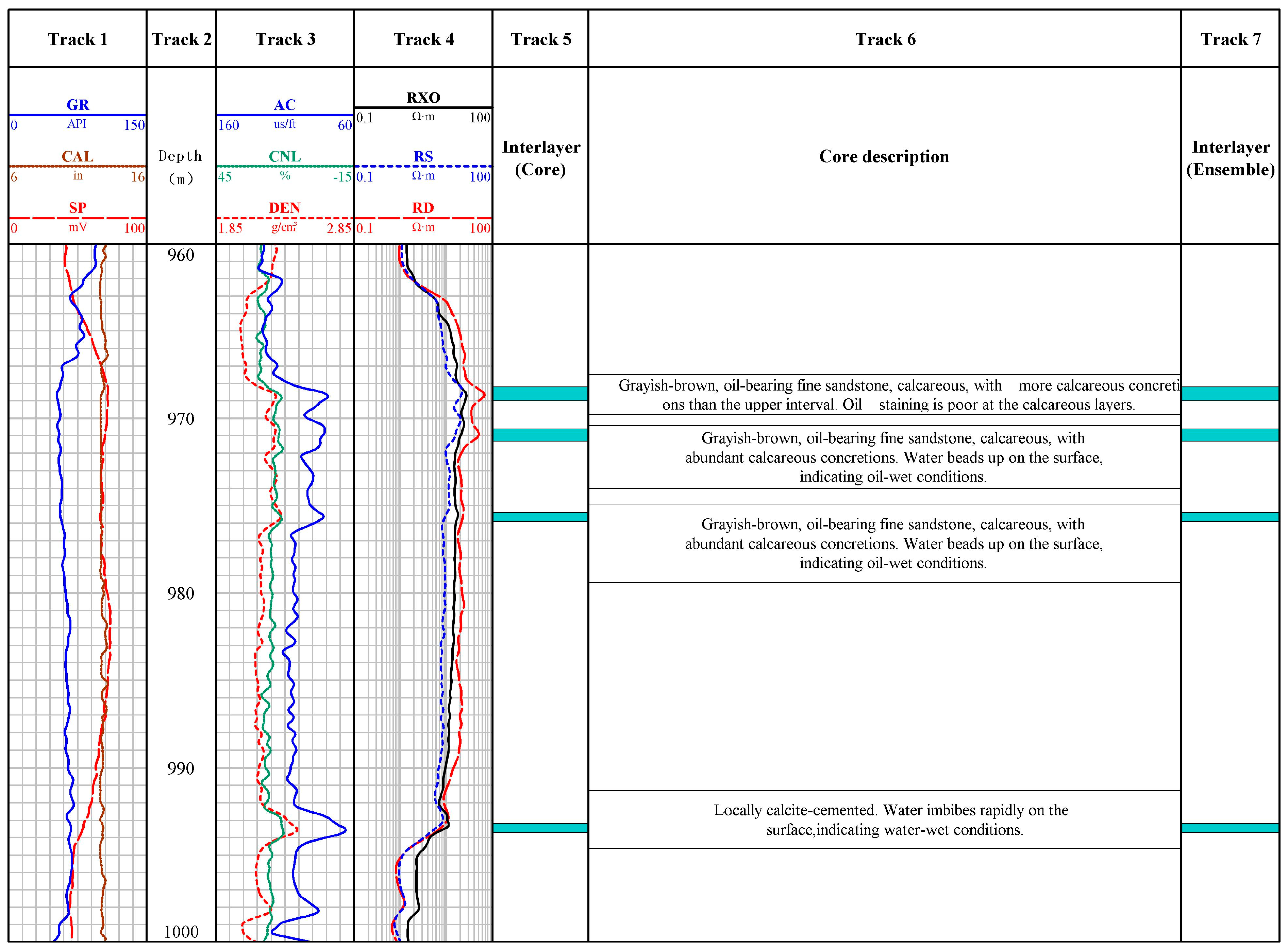
The above method is applied to the identification of a single well interlayer in the W Oilfield, and the interpretation results are shown in Figure 9. In Figure 9, the tracks are arranged as follows: Track 1 presents lithologic logging curves, including natural gamma ray (GR), spontaneous potential (SP), and well caliper (CAL); Track 2 corresponds to the depth scale (unit: m); Track 3 displays porosity-related logging curves, namely acoustic time difference (AC), density (DEN), and neutron (CNL); Track 4 shows resistivity logging data, consisting of deep resistivity (RD), shallow resistivity (RS), and flushed zone resistivity (RXO); Track 5 indicates the core-calibrated interlayer type; Track 6 presents detailed core description conclusions; and Track 7 displays the interlayer type identified by the SMOTE–ensemble learning method. The identification results are highly consistent with the core descriptions, verifying the method’s reliability in practical single well applications. The model is currently validated only on data from 14 wells in the W Oilfield. Reservoir properties (sedimentary environment, mineral composition) vary across regions, so its applicability to other geological settings requires further multi-oilfield and cross-well validation. The method’s effectiveness depends on the quality of original logging data—significant noise or outliers may reduce the reliability of synthetic samples. The framework is not tied to specific base learners, allowing researchers to easily replace or add other models (e.g., XGBoost, LightGBM) based on reservoir characteristics, with low computational complexity and strong practical operability.
Figure 9.
Interlayer identification result for WELL A.
4. Conclusions
Aimed at the problems of an unbalanced sample distribution and the limited accuracy of single machine learning models in interlayer identification in the W Oilfield, this study proposes a quantitative identification method integrating SMOTE and heterogeneous ensemble learning. The key conclusions are as follows:
Argillaceous, calcareous, and petrophysical interlayers in the W Oilfield exhibit distinct logging responses—calcareous interlayers are easily distinguishable via their high density and resistivity, while argillaceous and petrophysical interlayers are hard to differentiate by traditional methods due to their similar shale-bearing characteristics, highlighting the necessity of high-dimensional intelligent algorithms. The hybrid framework effectively addresses the core challenges: SMOTE synthesizes minority samples to balance data distribution, increasing the average accuracy of single models (KNN, DT, SVM) by 3.9%; the heterogeneous ensemble model with majority voting leverages algorithm complementarity, achieving a 92.6% accuracy on an untouched test set, and significantly enhancing the distinguishability between argillaceous and petrophysical interlayers and synchronously optimizing the macro F1-Score. This study provides a practical solution for accurate interlayer identification under small-sample and imbalanced conditions, offering reliable technical support for reservoir geological modeling and remaining oil potential tapping in the W Oilfield, and laying a foundation for the advancement of fine reservoir evaluation technology.
Future work will focus on two directions: integrating deep learning models (e.g., CNN, LSTM) to capture the spatial–temporal features of logging data, further improving the identification accuracy of interlayers with highly overlapping responses; optimizing SMOTE with hybrid sampling methods (e.g., SMOTE + undersampling) to mitigate overfitting risks in extreme imbalanced scenarios.
Author Contributions
Conceptualization, S.L., B.Y., T.Z., J.R., Q.Z., T.F. and J.Z.; methodology, S.L., B.Y., T.Z., J.R., Q.Z., T.F. and J.Z.; writing—original draft preparation, S.L., B.Y., T.Z., J.R., Q.Z., T.F. and J.Z.; writing—review and editing, S.L., B.Y., T.Z., J.R., Q.Z., T.F. and J.Z.; visualization, S.L.; supervision, S.L.; project administration, S.L. All authors have read and agreed to the published version of the manuscript.
Funding
This work was supported by the Natural Science Basic Research Program of Shaanxi (2024JC-YBMS-202).
Data Availability Statement
The data are contained within the article.
Acknowledgments
The authors have reviewed and edited the output and take full responsibility for the content of this publication.
Conflicts of Interest
Authors Shengqiang Luo, Tianrui Zhang and Qing Zeng were employed by the company Tarim Branch, China National Logging Corporation. Authors Bing Yu, Junqing Rong and Tingting Feng were employed by the company Geological Research Institute, China National Logging Corporation. The remaining authors declare that the research was conducted in the absence of any commercial or financial relationships that could be construed as a potential conflict of interest.
References
- Chen, L.; Yu, T.; Wang, C.; Yu, G.; Miu, J.; Xin, X.; Sun, K.; Tu, Z.; Li, G.; Zhao, X.; et al. Research on identification and quantitative characterization methods of separation and interlayer in sandstone reservoirs-Taking Taizhong 16 well area as an example. Geol. Rev. 2025, 71, 333–336. [Google Scholar] [CrossRef]
- Wang, W.; Dai, M.Y.; Chen, J.K.; Zou, Y.; Wu, Q.; Jiang, Q.; Feng, C. Identification and Distribution of Silurian Interlayers in YM 35 Well Block, Tarim Basin. Xinjiang Pet. Geol. 2025, 46, 154–162. [Google Scholar]
- Wang, J. Research on the Modeling of Interlayers in Reservoir. Master’s Thesis, China University of Petroleum (East China), Qingdao, China, 2010. [Google Scholar]
- Han, F.S. Study on Reservoir Heterogeneity and Interlayer of the Lower Member of Oficina Formation in the MPE-3 Block, Venezuela Basin. Master’s Thesis, China University of Petroleum (East China), Qingdao, China, 2017. [Google Scholar]
- Zhu, J.M.; Da, L.Y.; Gao, H.L. Identification of interlayers in sandy braided river reservoirs under less well conditions: A case study of LD2X oilfield, Bohai, China. Fault-Block Oil Gas Field 2020, 27, 739–744. [Google Scholar]
- Chen, H.L. Research on the Prediction Method of Interwell Interlayer in Donghe Sandstone of Hudson Oilfield. Master’s Thesis, China University of Petroleum (Beijing), Beijing, China, 2016. [Google Scholar]
- Dou, S.J.; Ji, L.; Wang, H.B.; Zhang, S.B.; Zhou, J. The Study of Interlayers within the Mesozoic Thick Oil Reservoirs in Wangguantun Oilfield. Pet. Geol. Eng. 2008, 22, 48–51. [Google Scholar] [CrossRef]
- Wu, J.; Fan, T.L.; Gao, Z.Q.; Li, C.; Zhang, T.; Ma, C. Identification, origin and distributions of barriers/baffles Xing-I oil layer in Block Du-84 of the western Liaohe Depression. Oil Gas Geol. 2017, 38, 248–258. [Google Scholar] [CrossRef]
- Yu, H.M.; Song, Y.C.; Peng, Y.T.; Bo, L.; Tong, L.; Kaibo, S. Characteristics, Genesis and Distribution of Interlayers in E31 Reservoir of Gasikule Oilfield, Qaidam Basin. Spec. Oil Gas Reserv. 2021, 28, 79–87. [Google Scholar] [CrossRef]
- Zhou, X.H.; Ding, W.L.; Chang, L.J. Three-end-mumber diagram of classification to identify the interlayers of sandstone reservoir in littoral facies: A case from Carboniferous Donghe sandstone in Hade Oil Field, Tarim Basin, NW China. Earth Sci. Front. 2017, 24, 328–338. [Google Scholar] [CrossRef]
- Shi, Z.H.; Zhang, J.L.; Li, M.; Gong, M.Z. Study on the development characteristics of the interlayer of Su6 block in Sulige gas field. China Sci. 2019, 14, 943–950. [Google Scholar] [CrossRef]
- Sun, N.Y. Study on the Interlayers of the Delta Front Reservoir in the Dongying Formation, SZ36-1 Oil Filed. Master’s Thesis, China University of Petroleum (Beijing), Beijing, China, 2021. [Google Scholar]
- Zhang, J.; Zhang, L.H.; Hu, S.Y.; Nan, Y.L. The Genesis and Characteristics and Identification of Intercalations in Non-marine Reservoir with Clastic Rock. Well Logging Technol. 2003, 27, 221–224. [Google Scholar] [CrossRef]
- Wang, N.; Zhang, L.P.; Feng, Y.G. Study on the distribution of the interlayers in Guantao-6 sand group of No.1 area in the central part of Gudao Oilfield. J. Xi’an Shiyou Univ. (Nat. Sci. Ed.) 2008, 23, 11–13. [Google Scholar] [CrossRef]
- Qu, Z.Y.; Luo, X.; Xie, R.C.; Ge, S.L.; Niu, H.L.; Yang, L. Application of WNN in the Studies of Interbeds. J. Oil Gas Technol. 2009, 31, 265–268. [Google Scholar] [CrossRef]
- Yi, S.; Wang, L.; Ni, J.E.; Chen, P.Y.; Li, C.; Sun, F.T. Characteristics and geological significance of interlayers in mixed reservoir of Asmari Formation in M oilfield. J. Xi’an Univ. Sci. Technol. 2021, 41, 1014–1024. [Google Scholar] [CrossRef]
- He, M.Q. Quantitative Study on Interlayer of Braided River Reservoir in High Water Cut Oilfield of DQ. Master’s Thesis, China University of Petroleum (Beijing), Beijing, China, 2020. [Google Scholar]
- Chen, H. Log Interpretation and Interlayers Identification in the Triassic Lower Oil Formation of the 9th Area and Block T903, Tahe Oilfield. Master’s Thesis, China University of Petroleum (Beijing), Beijing, China, 2021. [Google Scholar]
- Chen, Y.; Jiao, S.X.; Cheng, C.; Huang, C.; Jiang, Y.Q. Semi-Supervised Interlayer Identification Method Based on Self-Encoder. Spec. Oil Gas Reserv. 2021, 28, 86–91. [Google Scholar] [CrossRef]
- Zheng, Z.C. Research and Application of Recognition Algorithm of Interlayer in Reservoir Based on Convolution Neural Network. Master’s Thesis, Xi’an Shiyou University, Xi’an, China, 2021. [Google Scholar]
- Chawla, N.V.; Bowyer, K.W.; Hall, L.O.; Kegelmeyer, W.P. SMOTE: Synthetic minority over-sampling technique. J. Artif. Intell. Res. 2002, 16, 321–357. [Google Scholar] [CrossRef] [Scilit]
- Zhou, K.; Zhang, J.; Ren, Y.; Huang, Z.; Zhao, L. A gradient boosting decision tree algorithm combining synthetic minority oversampling technique for lithology identification. Geophysics 2020, 85, WA147–WA158. [Google Scholar] [CrossRef] [Scilit]
- Ibrahim, B.; Ahenkorah, I.; Ewusi, A.; Majeed, F. A Novel XRF-Based Lithological Classification in the Tarkwaian Paleo Placer Formation Using SMOTE-XGBoost. J. Geochem. Explor. 2023, 245, 107–147. [Google Scholar] [CrossRef] [Scilit]
- Deng, S.; Pan, H.; Li, C.; Yan, X.; Wang, J.; Shi, L.; Pei, C.; Cai, M. A Real-Time Lithological Identification Method Based on SMOTE-Tomek and ICSA Optimization. Acta Geol. Sin.-Engl. Ed. 2024, 98, 518–530. [Google Scholar] [CrossRef] [Scilit]
- Song, C.; Zhao, T.; Xu, L.; Huang, X. Probabilistic Prediction of Uniaxial Compressive Strength for Rocks from Sparse Data Using Bayesian Gaussian Process Regression with Synthetic Minority Oversampling Technique (SMOTE). Comput. Geotech. 2024, 165, 105850. [Google Scholar] [CrossRef] [Scilit]
- Hu, C.; Deng, R.; Hu, X.; He, M.; Zhao, H.; Jiang, X. An Automatic Methodology for Lithology Identification in a Tight Sandstone Reservoir Using a Bidirectional Long Short-Term Memory Network Combined with Borderline-SMOTE. Acta Geophys. 2025, 73, 2319–2335. [Google Scholar] [CrossRef] [Scilit]
- Yao, H.; Liang, M.; Yin, S.; Zhang, Q.; Tian, Y.; Wang, G.; Hou, E.; Lian, H.; Zhang, J.; Wu, C. Application of Hybrid Model Based on LASSO-SMOTE-BO-SVM to Lithology Identification During Drilling. Processes 2025, 13, 2038. [Google Scholar] [CrossRef] [Scilit]
- Tan, M.J.; Bai, Y.; Wu, J.; Zhang, H.T.; Li, G.R.; Xiao, C.W.; Han, C.; Wei, M.P. Progress of research on committee machine logging interpretation methods driven by multi-source data. Geophys. Prospect. Pet. 2022, 61, 224–235. [Google Scholar] [CrossRef]
- Wang, D.; Cheng, H.L.; Ding, W.N.; Li, D.; Liu, H. Application of SVR and AdaBoosting arithmetic in porosity interpretation of porous carbonate reservoir. Prog. Geophys. 2023, 38, 2576–2587. [Google Scholar] [CrossRef]
- Bai, Y.; Tan, M.J.; Xiao, C.W.; Han, C.; Wu, H.; Luo, W.; Xu, B. Dynamic classification committee machine-based fluid typing method from wireline logs for tight sandstone gas reservoir. Chin. J. Geophys. 2021, 64, 1745–1758. [Google Scholar] [CrossRef]
- Tan, M.; Bai, Y.; Zhang, H.; Li, G.; Wei, X.; Wang, A. Fluid typing in tight sandstone from wireline logs using classification committee machine. Fuel 2020, 271, 117601. [Google Scholar] [CrossRef] [Scilit]
- Bai, Y.; Tan, M. Dynamic committee machine with fuzzy-c-means clustering for total organic carbon content prediction from wireline logs. Comput. Geosci. 2020, 146, 104626. [Google Scholar] [CrossRef] [Scilit]
- Hong, W.J. Research on the Method of Quantitative Identification of Interbed in Lamadian Oilfeld. Master’s Thesis, China University of Petroleum (East China), Qingdao, China, 2019. [Google Scholar]


Disclaimer/Publisher’s Note: The statements, opinions and data contained in all publications are solely those of the individual author(s) and contributor(s) and not of MDPI and/or the editor(s). MDPI and/or the editor(s) disclaim responsibility for any injury to people or property resulting from any ideas, methods, instructions or products referred to in the content. |
© 2026 by the authors. Licensee MDPI, Basel, Switzerland. This article is an open access article distributed under the terms and conditions of the Creative Commons Attribution (CC BY) license.