Hierarchically Weighted Evidence for Fuzzy–Probabilistic Carbon Footprint Uncertainty Analysis

Abstract

Accurate carbon footprint accounting is essential for advancing carbon management and optimising energy systems. However, existing uncertainty analyses are often difficult to reproduce and interpret because the underlying evidence is scattered across multiple sources, thereby making it hard to attribute uncertainty to specific drivers. To address this gap, we propose a transparent uncertainty quantification framework that (i) distills multi-source evidence into auditable rules, (ii) propagates ambiguity through fuzzy aggregation, and (iii) maps interval outputs to probabilistic representations for scenario-based Monte Carlo simulation. In the case study, the proposed method yields more stable carbon footprint estimates than conventional approaches, with lower variability across repeated simulations, and it enables clearer uncertainty attribution by separating random variation from structural uncertainty. Overall, this paper provides a traceable and interpretable method for high-precision uncertainty quantification in carbon footprint assessment.

1. Introduction

In the context of carbon peaking and carbon neutrality goals, carbon footprint accounting has become a key instrument for enterprise carbon management, energy system optimisation, and Life Cycle Assessment (LCA) [1,2]. Whether controlling emissions during manufacturing or optimising supply chains toward low-carbon outcomes, decision-making and policy design increasingly rely on accurate emission quantification with explicit uncertainty characterisation [3]. As low-carbon transformation expands across sectors, carbon footprint assessment is shifting from single-stage or single-source accounting to multi-source evidence integration and uncertainty propagation in complex systems [4]. However, practical applications are often constrained by approximate inputs, ambiguous system boundaries, and limited interpretability of algorithmic models, making robust and transparent uncertainty assessment a central challenge [2,5].

As a widely used indicator for evaluating the emission scale of greenhouse gases, the carbon footprint has been extensively studied across products, industries, cities, and nations [6,7,8,9,10]. Prior work has established core methodological paradigms and clarified boundary and data requirements. Meanwhile, uncertainty has received growing attention due to heterogeneity in activity data, emission factors, and boundary assumptions, as well as differences in accounting perspectives and regional contexts [11]. Recent reviews further highlight persistent obstacles such as the lack of industry standards and challenges in real-time tracking [12]. To quantify uncertainty, Monte Carlo Simulation (MCS) and related resampling approaches are increasingly adopted [13,14,15], including applications in metropolitan sectoral footprints [16]. Despite their usefulness, existing practices still face unresolved issues in parameter specification, distributional assumptions, and interpretable reporting of results.

Overall, current carbon footprint uncertainty accounting remains limited in three aspects. (1) Traditional stage-by-stage approaches are time-consuming and often struggle with linguistic or scenario-based fuzzy uncertainty commonly encountered in complex systems [17]. (2) Many uncertainty workflows cannot efficiently incorporate unstructured and multi-source evidence and rarely distinguish evidence by authority or timeliness, which weakens the reliability of integrated estimates [18]. (3) The mapping from fuzzy linguistic descriptions to probabilistic representations is frequently based on subjective settings, undermining the accuracy and credibility of uncertainty propagation [19].

To address these problems, this study proposes a method for carbon footprint uncertainty calculation based on a truncated normal distribution and fuzzy interval weighting. Its core lies in constructing a three-stage transparent rule reasoning framework: evidence distillation, fuzzy synthesis, and interval extraction. This framework achieves a dynamic fusion of multi-source evidence and uncertainty quantification. We use a large language model (LLM) to extract rules from multi-source data and construct an auditable rule base for traceable reasoning. By leveraging truncated normal distributions, it achieves an accurate alignment between fuzzy intervals and the probabilistic model. This approach effectively addresses the limitations of traditional methods in adapting to fuzzy uncertainties, integrating multi-source data, ensuring algorithmic interpretability, and improving mapping accuracy. Accordingly, our proposed method provides a precise solution for quantifying carbon footprint uncertainty, which is relevant in scenarios such as carbon management in manufacturing processes and energy system optimisation. Compared with existing fuzzy–probabilistic approaches, our novelty is that the fuzzy-to-probabilistic mapping is constrained by an auditable rule base distilled from multi-source evidence, reducing reliance on ad hoc subjective settings. Compared with two-dimensional Monte Carlo frameworks, we provide a more traceable and interpretable workflow that separates evidence-driven structural ambiguity from random variation before scenario-based simulation.

The main contributions of the study are outlined as follows:

• We propose a transparent uncertainty-quantification workflow for carbon footprint assessment that integrates evidence-credibility weighting, fuzzy interval reasoning, and probabilistic propagation under explicit boundary constraints.
• We introduce an LLM-assisted evidence distillation mechanism that converts multi-source evidence into a structured rule base with traceable weights, enabling auditable links from evidence to rules and uncertainty outputs.
• We develop a reproducible mapping from fuzzy results to sampleable probabilistic representations under explicit bounds, and combine three-scenario conditional Monte Carlo simulation with variance decomposition to separate random variability from structural uncertainty.

2. Methodology

2.1. Overall

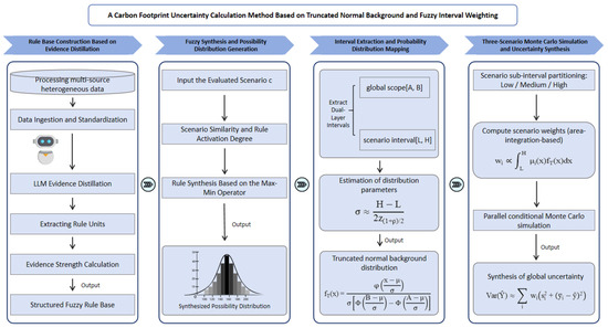
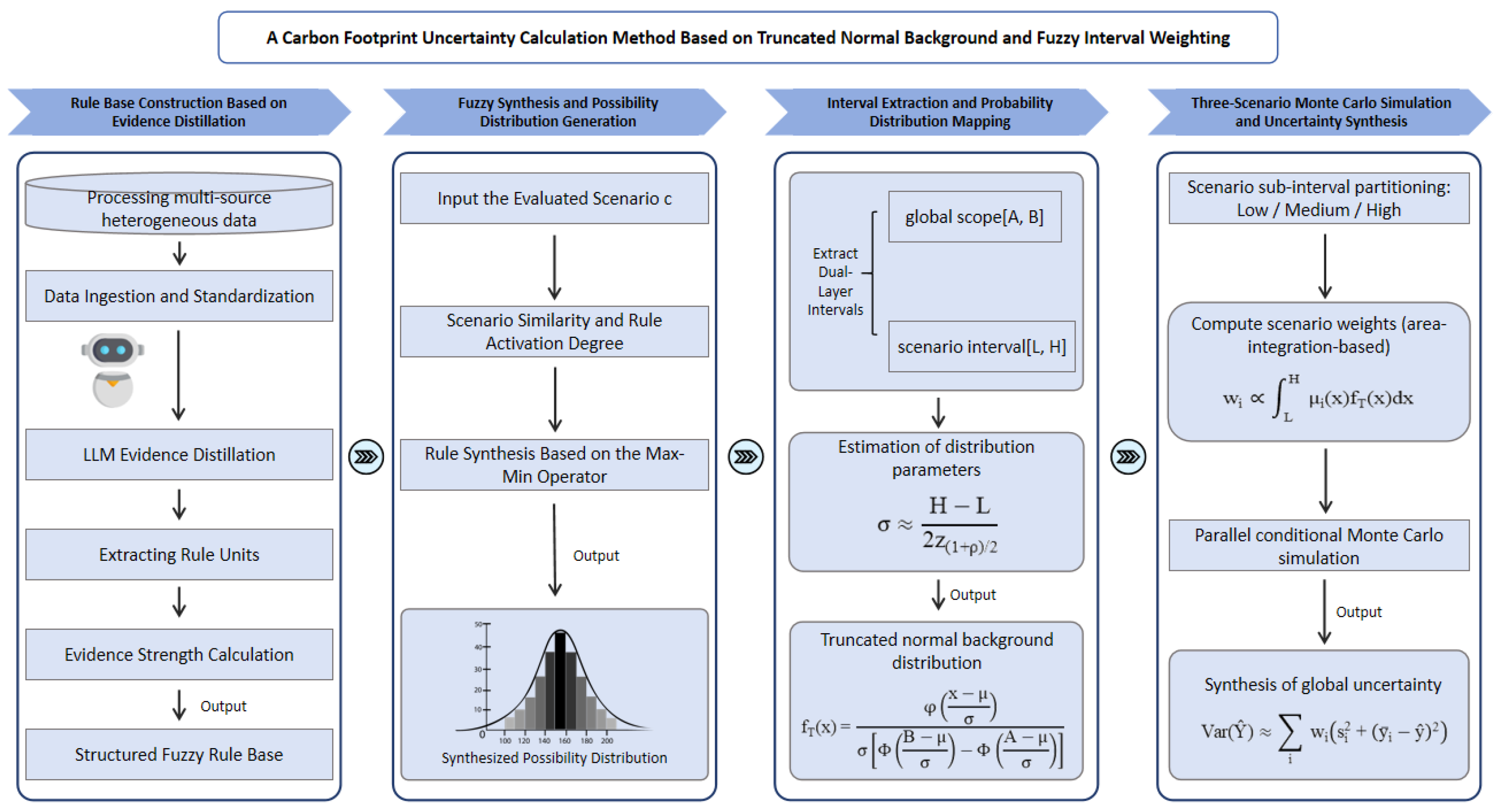
In this section, we present a novel approach for quantifying carbon footprint uncertainty that combines a truncated normal prior with fuzzy interval weighting, thereby addressing key limitations of conventional assessments. This method maps qualitative linguistic descriptions into quantitative probability distributions. It integrates LLM-based evidence distillation, fuzzy-logic-based rule synthesis, and Monte Carlo-based probability propagation [20]. The overall technical approach is illustrated in Figure 1.

Figure 1. Overall Technical Roadmap, which is divided into four interconnected core stages.

• Rule Base Construction and Evidence Distillation: Traditional carbon-footprint assessments often rely on information that is dispersed across heterogeneous sources and presented in unstructured or semi-structured formats. As a result, manual curation becomes inefficient, error-prone, and difficult to evaluate in terms of reliability. To address these issues, we employ an LLM to distill source content into structured fuzzy rules and assign credibility-aware weights to each rule. This module reduces manual curation effort and provides auditable inputs for subsequent uncertainty quantification.
• Fuzzy Synthesis and Probability Distribution Generation: Rule applicability varies across scenarios, and treating rules in isolation can yield scenario-dependent bias. To mitigate this risk, we activate the relevant rules and aggregate multiple evidence streams using fuzzy operators. This step resolves conflicts while retaining complementary evidence across them. It further converts discrete fuzzy rules into a continuous possibility distribution to enable quantitative analysis.
• Interval Extraction and Probability Distribution Mapping: A possibility distribution cannot be sampled directly in Monte Carlo simulation. Therefore, we first extract the global boundaries and a high-confidence interval to remove infeasible and low-credibility regions. We then convert these constraints into a truncated normal probability distribution using the maximum entropy principle [21,22]. This module provides a theoretically grounded mapping from a fuzzy possibility distribution to a sampleable probability distribution.
• Three-Scenario Monte Carlo Simulation and Uncertainty Synthesis: A conventional single-interval simulation may obscure regime-specific variability and yield unstable estimates. Accordingly, we partition the high-confidence interval into three subscenarios, namely low, medium, and high confidence, and run conditional Monte Carlo simulations for each subscenario. Finally, we synthesize the results using variance-based weighting via the law of total variance, yielding estimates of the mean carbon footprint and its associated uncertainty in a unified manner.

2.2. Rule Base Construction Based on Evidence Distillation

A high-quality, structured rule repository forms the basis of the proposed uncertainty assessment framework. This module aims to consolidate multi-source and heterogeneous inputs into standardized rule units, which in turn enables consistent fuzzy inference in subsequent stages. To achieve this goal, we implement a two-stage pipeline. First, we collect data from multiple sources and standardize their formats and semantics to ensure comparability. Second, we employ an LLM to extract candidate rules from the standardized data and normalize them into a unified representation suitable for rule activation and fuzzy synthesis.

2.2.1. Data Acquisition and Standardization

The data used in this study come from diverse sources, including historical production records, authoritative industry reports, peer-reviewed papers, and expert knowledge texts. Because these sources differ in format, granularity, and measurement conventions, we apply rigorous acquisition and standardization procedures to ensure data consistency and validity prior to modeling.

A major source of inconsistency arises from unit mismatches. The same parameter is often reported in different units across sources, and untreated discrepancies can propagate systematic errors into subsequent estimation and evaluation. To address this issue, we convert all measurements using a curated data dictionary that specifies admissible units and conversion factors for each parameter. This procedure harmonizes measurement standards across sources and preserves numerical comparability in downstream analyses.

In addition, we address boundary violations and anomalous observations that can bias parameter estimates. We use physical boundary checks to identify records that are physically implausible and remove or flag them accordingly. For statistical outliers, we apply tail trimming rather than direct exclusion, which reduces the influence of extreme values while retaining distributional information and sample size. These preprocessing steps collectively improve the robustness of parameter estimation and provide more reliable inputs for uncertainty quantification.

2.2.2. LLM Rule Extraction and Normalization

Traditional approaches typically rely on domain experts to manually construct rule repositories, which introduces several practical limitations. In practice, expert curation requires substantial time and labor, and the resulting rule sets may reflect subjective judgments. More importantly, manual workflows do not scale with the volume and heterogeneity of multi-source inputs, which makes them ill-suited for large-scale carbon footprint analysis.

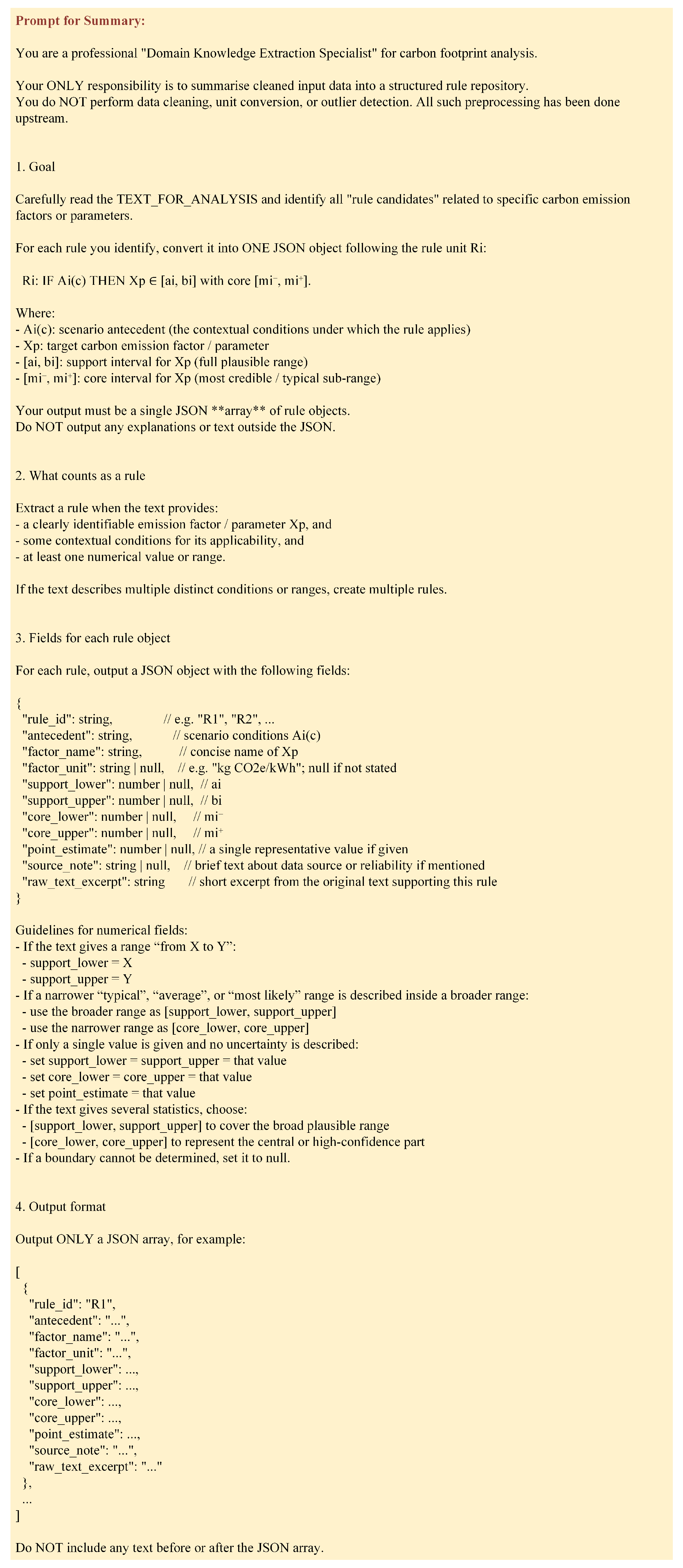
To overcome these limitations, we use large language models (LLMs) as knowledge-engineering tools and couple them with prompt-engineering strategies (see Appendix A). Specifically, the LLM extracts rule-relevant evidence from unstructured text and converts it into standardized rule expressions. This design reduces manual effort, mitigates subjective bias, and improves scalability for multi-source data processing. Concretely, we design prompt templates that instruct the LLM to identify rule candidates associated with specific carbon emission factors in the input text. The LLM then outputs each candidate as a structured rule unit in a consistent format, which facilitates downstream rule activation and fuzzy synthesis while maintaining a unified representation across sources.

Rule $R_i$ is defined as:

$$R_i:\mathbf{IF}{A}_i\left(\mathbf{c}\right)\mathbf{THEN}{X}_p\sim {\tilde{N}}_i,{\tilde{N}}_i=(a_i,m_i^{-},m_i^{+},b_i),w_i\in [0,1],$$

(1)

where $A_i\left(\mathbf{c}\right)$ denotes the antecedent describing the contextual conditions for which the rule applies. The consequent $X_p$ is represented by a trapezoidal fuzzy number ${\tilde{N}}_i$ whose support is $[a_i,b_i]$ and core is $[m_i^{-},m_i^{+}]$ (with $a_i\le m_i^{-}\le m_i^{+}\le b_i$). The weight $w_i$ quantifies the evidence strength (credibility) of rule $R_i$. The evidence strength ${\mathrm{w}}_{\mathrm{i}}$ is defined as follows:

$${\mathrm{w}}_{\mathrm{i}}=\underset{\mathrm{source}\mathrm{authority}}{\underbrace{{\mathrm{S}}_{\mathrm{src}}}}\times \underset{\mathrm{timeliness}}{\underbrace{{\mathrm{e}}^{-\lambda ·{\mathrm{age}}_{\mathrm{i}}}}}\times \underset{\mathrm{consistency}}{\underbrace{{\mathrm{S}}_{\mathrm{cons}}}}\times \underset{\mathrm{quality}·\mathrm{score}}{\underbrace{{\mathrm{S}}_{\mathrm{quality}}}},$$

(2)

where source authority follows a predefined hierarchy, whereas timeliness down-weights stale evidence through an exponential decay function parameterized by the publication age and a decay coefficient. Consistency reflects agreement with similar evidence in the knowledge base, and the quality score aggregates study-level attributes such as sample size and data-collection methodology.

Evidence strength governs the contribution of each rule during the subsequent synthesis stage. Because a single indicator cannot capture rule credibility in a comprehensive and objective manner, we compute rule weights by integrating four dimensions, namely source authority, timeliness, consistency, and quality score. Together, these dimensions reflect reliability, currency, cross-source agreement, and scientific validity, which reduces the bias introduced by single-dimensional weighting. As a result, the influence assigned to each rule better matches its underlying credibility, providing a principled basis for accurate fuzzy synthesis in later steps.

2.3. Fuzzy Synthesis and Possibility Distribution Generation

Building on the structured rule repository, this phase aims to activate scenario-relevant rules for a given scenario c and to aggregate potentially conflicting or complementary evidence into a unified possibility distribution $\pi \left(x\right)$ for the target parameter x.

2.3.1. Scenario Similarity and Rule Activation Degree Calculation

To quantify how well each rule ${\mathrm{R}}_i$ in the rule base matches the current evaluation scenario c, we compute its activation degree. This computation begins by measuring scenario similarity. For each scenario dimension d, we define a Gaussian-decay similarity function $s_d\in [0,1]$ as follows:

$$s_d=exp\left(-{\displaystyle \frac{{\left(c_d-A_{i,d}\right)}^2}{2{\tau }_d^{2w}}}\right),$$

(3)

where ${\mathrm{c}}_{\mathrm{d}}$ denotes the current scene’s value in dimension d, and ${\mathrm{A}}_{\mathrm{i},\mathrm{d}}$ represents rule i’s anchor value in that dimension. ${\tau }_{\mathrm{d}}$ is the sensitivity coefficient controlling the decay rate. When the dimension value in the rule’s antecedent perfectly matches the current scene, ${\mathrm{s}}_{\mathrm{d}}=1$; otherwise, it decays according to the degree of discrepancy.

Subsequently, the fuzzy rule i determines its overall activation level ${\gamma }_i\left(c\right)$ by aggregating the dimension-wise similarities using the Minimum Operator. Consistent with the barrel-effect principle, this operator assumes that the overall activation is governed by the weakest-matching dimension, thereby yielding a conservative yet robust measure. Formally, the activation level is given by

$${\gamma }_i\left(c\right)=\underset{d}{min}{s}_d.$$

(4)

In practical applications, rules in the rule repository exhibit varying degrees of adaptability to specific scenarios. Therefore, we avoid indiscriminately applying all rules when computing the results for the current scenario, since doing so may introduce substantial irrelevant information and consequently bias the evaluation. Moreover, when partial dimensional information is missing, we adopt a weight-reduction strategy to prevent unreasonable rule overactivation. For example, we explicitly set the similarity of any missing dimension to zero or to a small predefined value.

By computing scenario similarity and rule activation levels, we further filter the rule set and retain only those rules that are most consistent with the current scenario. In addition, we allow the use of diverse distance metrics and activation aggregation strategies to accommodate cross-scenario variability in dimensional features, thereby ensuring that the activated rules remain aligned with the current evaluation requirements. As a result, we improve the relevance of the subsequent synthesis outcomes.

2.3.2. Fuzzification of Parameter Intervals

To process parameter information of varying forms within a unified framework, we convert such information into membership functions. Specifically, a membership function maps any parameter value x to the interval $[0,1]$, where the resulting value indicates the degree to which x satisfies the interval specified by rule i. Among various choices, we adopt the trapezoidal membership function, as it is widely used in practice and its parameters naturally correspond to the support set and the core band of a rule unit:

$${\mu }_i\left(x\right)=\left\{\begin{array}{cc}0,\hfill & x\le a_i\hfill \\ {\displaystyle \frac{x-a_i}{m_i^{-}-a_i}},\hfill & a_i<x<m_i^{-}\hfill \\ 1,\hfill & m_i^{-}\le x\le m_i^{+}\hfill \\ {\displaystyle \frac{b_i-x}{b_i-m_i^{+}}},\hfill & m_i^{+}<x<b_i\hfill \\ 0,\hfill & x\ge b_i\hfill \end{array}\right..$$

(5)

Parameter representations in the rule base are heterogeneous, including point values, intervals, and other forms. Since such heterogeneous parameters cannot be directly handled under a unified synthesis operation, we transform them into membership functions. This transformation enables us to map diverse parameter descriptions onto a standardized credibility interval $[0,1]$, thereby explicitly quantifying the credibility associated with different parameter values. Moreover, by representing heterogeneous parameters in a unified functional form, we establish a consistent computational basis for subsequent fuzzy-logic-based synthesis, effectively mitigating the fusion challenges induced by parameter heterogeneity.

With this formulation, we interpret the resulting membership function in an intuitive manner: values within the core band are regarded as fully credible, values at the boundary of the support set are marginally credible, and values outside the support set are non-credible. In the special case where the core band collapses to a single point, i.e., ${\mathrm{m}}_{\mathrm{i}}^{-}={\mathrm{m}}_{\mathrm{i}}^{+}={\mathrm{m}}_{\mathrm{i}}$, we obtain the degenerated form of the function, which is typically expressed as:

$${\mu }_i\left(x\right)=\left\{\begin{array}{cc}0,\hfill & x\le a_i\hfill \\ {\displaystyle \frac{x-a_i}{m_i-a_i}},\hfill & a_i<x\le m_i\hfill \\ 1,\hfill & x=m_i\hfill \\ {\displaystyle \frac{b_i-x}{b_i-m_i}},\hfill & m_i<x<b_i\hfill \\ 0,\hfill & x\ge b_i\hfill \end{array}\right..$$

(6)

2.3.3. Rule Synthesis Based on the Max–Min Operator

This step constitutes the core of our fuzzy reasoning procedure. Specifically, we synthesize all activated rules and their associated evidence strengths into a single, comprehensive possibility distribution. To this end, we adopt a weighted Max–Min composition operator:

$$\pi \left(x\right)=\underset{i}{max}min\left({\gamma }_i\left(c\right)·w_i,{\mu }_i\left(x\right)\right),$$

(7)

where ${\mu }_i\left(x\right)$ denotes the membership degree induced by rule i, characterizing the extent to which a given value x is supported by that rule. Moreover, ${\gamma }_i\left(c\right)·w_i$ is the weighted activation degree of rule i, which jointly accounts for its scenario-dependent applicability ${\gamma }_i\left(c\right)$ and its evidence strength $w_i$.

For clarity, we decompose the above computation into the following steps:

• Weighted activation. For each rule i, we compute its composite influence by multiplying its activation under the current scenario, ${\gamma }_i\left(c\right)$, with the corresponding evidence strength $w_i$, yielding ${\gamma }_i\left(c\right)·w_i$.
• Rule-wise truncation. For each rule i, we take the minimum between its weighted activation ${\gamma }_i\left(c\right)·w_i$ and its membership function value ${\mu }_i\left(x\right)$, i.e., $min({\gamma }_i\left(c\right)·w_i,{\mu }_i\left(x\right))$, which effectively limits the rule’s contribution at each x.
• Aggregation across rules. Finally, we apply a pointwise maximum over all truncated rule outputs to obtain the resulting possibility distribution $\pi \left(x\right)$.

In practice, multiple activated rules may exhibit complementary or conflicting relationships; thus, directly superimposing their outputs may yield inconsistent results. By construction, the $min(·)$ operation caps each rule’s contribution using the weighted activation as an upper bound, whereas the $max(·)$ operation selects the dominant contribution at each x. This fusion emphasizes rules that are both scenario-relevant and well supported by evidence, while limiting interference among conflicting rules, yielding a single possibility distribution $\pi \left(x\right)$.

2.4. Range Extraction and Probability Distribution Mapping

An explicit conversion mechanism is required to convert the fuzzy possibility distribution $\pi \left(\mathrm{x}\right)$ into a probability distribution suitable for Monte Carlo simulation. This stage accomplishes the conversion by extracting key intervals and conducting probability mapping.

2.4.1. Extraction of Global and Scenario-Specific Ranges

To comprehensively describe parameter uncertainty, we extract two distinct levels of intervals from the $\pi \left(\mathrm{x}\right)$:

• Global range $[\mathit{A},\mathit{B}]$. To delineate the practically meaningful domain of a parameter while suppressing spurious tails induced by model or data noise, we define the global range as the smallest interval that covers the $ϵ$-cut of the possibility distribution:

  $$[A,B]=\mathrm{the}\mathrm{smallest}\mathrm{interval}\mathrm{covering}\{x\mid \pi (x)>ϵ\},$$

  (8)

  where $ϵ$ is a near-zero threshold used to discard regions with extremely low credibility. Because possibility distributions often exhibit long low-credibility tails, including these tail regions in subsequent analyses may degrade estimation accuracy. By extracting $[A,B]$, we retain all practically meaningful candidate values while filtering out implausible noise, which in turn provides valid truncation boundaries for the subsequent probability distribution construction.
• Contextual range $[\mathit{L},\mathit{H}]$. Although the global range $[A,B]$ captures all plausible values, it may remain overly broad and thus obscure the core characteristics of the parameter distribution. Therefore, we further extract a high-confidence operational range in which the parameter is most likely to occur. Given a predefined coverage rate $\rho$ (typically $90\%$ or $95\%$), we determine a confidence threshold ${\alpha }^{*}$ such that the corresponding $\alpha$-cut attains the desired coverage while remaining as compact as possible:

  $${\alpha }^{*}=\underset{\alpha }{max}\alpha \mathrm{s}.\mathrm{t}.{\displaystyle \frac{\lambda \left(\{x\mid \pi (x)\ge \alpha \}\right)}{\lambda \left(\right[A,B\left]\right)}}\ge \rho ,$$

  (9)

  where $\lambda (·)$ denotes the interval length (Lebesgue measure). After obtaining ${\alpha }^{*}$, we define the contextual range $[L,H]$ as the smallest interval covering $\{x\mid \pi \left(x\right)\ge {\alpha }^{*}\}$. For multimodal $\pi \left(x\right)$, to avoid information loss, we preserve the high-confidence regions associated with major peaks by extracting a union of locally bounded intervals (i.e., multiple disjoint sub-intervals) rather than collapsing them into a single interval.

2.4.2. Mapping to Truncated Normal Distribution

To enable Monte Carlo propagation, the synthesized possibility distribution $\pi \left(x\right)$ is mapped to a bounded, sampleable probability model over the physically admissible range $[A,B]$. We adopt a truncated normal distribution because, for the key parameters considered in this study, $\pi \left(x\right)$ is approximately unimodal and near-symmetric. While the broader methodology discusses multimodal cases for completeness, the evidence in the present study does not warrant more complex representations. Accordingly, we use the truncated normal model for its transparency and reproducibility: its location and scale are determined directly from the high-confidence interval $[L,H]$ at the prescribed coverage level $\rho$. Truncation to $[A,B]$ further enforces physical feasibility, ensuring that uncertainty propagation is governed by evidence-based constraints rather than by unrealistic extreme values.

Standard deviation $\sigma$: Based on the assumption that [L, H] is the confidence interval with coverage $\rho$.

$$\sigma \approx {\displaystyle \frac{\mathrm{H}-\mathrm{L}}{2{\mathrm{z}}_{(1+\rho )/2}}}\left(\rho =0.95,{\mathrm{z}}_{0.975}\approx 1.96\right).$$

(10)

Thus, we obtain a truncated normal distribution defined on the interval [A, B] with a high-density region [L, H], denoted as ${\mathrm{f}}_{\mathrm{T}}\left(\mathrm{x}\right)$. Its probability density function (PDF) is expressed as follows:

$${\mathrm{f}}_{\mathrm{T}}\left(\mathrm{x}\right)={\displaystyle \frac{\phi \left(\frac{\mathrm{x}-\mu }{\sigma }\right)}{\sigma \left[\mathrm{\Phi }\left(\frac{\mathrm{B}-\mu }{\sigma }\right)-\mathrm{\Phi }\left(\frac{\mathrm{A}-\mu }{\sigma }\right)\right]}},$$

(11)

where $\phi \left(\mathrm{x}\right)$ and $\mathrm{\Phi }\left(\mathrm{x}\right)$ denote the probability density function and cumulative distribution function of the standard normal distribution, respectively.

2.5. Three-Scenario Monte Carlo Simulation and Uncertainty Synthesis

Finally, through refined scenario partitioning for parameter distributions and weighted Monte Carlo simulations, uncertainty is accurately propagated and ultimately integrated within computational graphs, where the graphs systematically fuse the probabilistic inputs of all parameters to output the overall uncertainty of the model.

2.5.1. Scenario Sub-Interval Partitioning and Fuzzy Weight Calculation

Since Monte Carlo simulations based on a single high-confidence interval cannot capture the heterogeneous effects of different value ranges on the carbon footprint, we further refine the contextual range $[L,H]$ by partitioning it into three scenarios, namely low, medium, and high. Concretely, we adopt an equal-width partition:

$$\mathrm{\Delta }={\displaystyle \frac{H-L}{3}},I_1=[L,L+\mathrm{\Delta }],I_2=[L+\mathrm{\Delta },L+2\mathrm{\Delta }],I_3=[L+2\mathrm{\Delta },H].$$

(12)

Rationale for using a (truncated) normal background distribution. To translate the synthesized possibility distribution into a probabilistic form suitable for Monte Carlo sampling, we introduce a data-informed background density $f_T\left(x\right)$ on the credible domain. We model this background density as a truncated normal distribution for three reasons. First, aggregated evidence effects are often well approximated by a unimodal, Gaussian-shaped variability, providing a smooth baseline centered around a typical value. Second, truncation enforces credible bounds (e.g., $[A,B]$ or $[L,H]$) and prevents samples from drifting into low-credibility tail regions. Third, the truncated normal is computationally convenient: interval masses can be evaluated efficiently and stably, which is beneficial for repeated sampling and weighting.

Rationale for three-way partition of $[L,H]$. We partition $[L,H]$ into three subranges to align with the standard fuzzy semantic discretization of continuous domains into three linguistic terms (Low/Medium/High), which offers a principled trade-off between interpretability and granularity. Using only two partitions would be insufficient to represent a neutral “medium” regime, whereas a finer partition would increase scenario complexity without commensurate interpretability gains. The resulting tripartite structure therefore provides a concise yet expressive basis for attributing uncertainty contributions to distinct value regimes.

Why equal-width rather than equal-probability partition. Importantly, we employ equal-width splitting rather than equal-probability splitting. An equal-probability partition would assign identical probability mass to each scenario by construction, thereby obscuring distributional heterogeneity and weakening the interpretability of scenario-specific impacts. In contrast, equal-width partitioning fixes the geometric domain consistently and allows the background density to determine the scenario weights endogenously.

Accordingly, given the truncated normal background density $f_T\left(x\right)$, we compute the scenario masses and normalized scenario weights as

$$p_i={\int }_{I_i}{f}_T\left(x\right)dx,$$

(13)

$${\omega }_i={\displaystyle \frac{p_i}{{\sum }_{j=1}^3{p}_j}}.$$

(14)

To further preserve smooth fuzzy transitions and mitigate discontinuities induced by hard interval boundaries, we extend the area-based weighting to a fuzzy-semantic form by weighting the density with the corresponding membership function:

$${\omega }_j={\displaystyle \frac{{\int }_L^H{\nu }_j\left(x\right)f_T\left(x\right)dx}{{\sum }_{k=1}^3{\int }_L^H{\nu }_k\left(x\right)f_T\left(x\right)dx}}.$$

(15)

When ${\nu }_j\left(x\right)$ degenerates to a rectangular function over $I_j$, the above formulation reduces to the area method, i.e., ${\omega }_j\propto {\int }_{I_j}{f}_T\left(x\right)dx$.

2.5.2. Conditional Sampling and Parallel Simulation

For the low–medium–high scenarios, we perform conditional sampling by drawing truncated samples within the corresponding subinterval $I_i$. In each run, samples are drawn exclusively from $I_i$ for scenario i. To improve comparability across scenarios, we use common random numbers (CRN) by matching random seeds and sample sizes across the three scenarios while evaluating each scenario separately. For scenario i, we obtain the sample mean ${\overline{y}}_i$ and sample variance $s_i^2$ of the carbon footprint. Under the matched-seed and matched-budget design, differences in ${\overline{y}}_i$ and $s_i^2$ primarily reflect the effect of the scenario-specific parameter range rather than sampling variability. These scenario-wise statistics are then used as inputs to the subsequent global synthesis.

2.5.3. Weighted Synthesis and Final Uncertainty Output

In the final step, we weight and synthesize the simulation outputs from the three scenarios to derive the global carbon footprint estimate and its overall uncertainty.

Global mean. We aggregate the three scenario-specific mean estimates into a single global mean via a weighted average, where ${\omega }_i$ indicates the relative contribution of scenario i and ${\sum }_{i=1}^3{\omega }_i=1$.

$$\widehat{y}=\sum _{i=1}^3{\omega }_i{\overline{y}}_i.$$

(16)

Global variance. According to the law of total variance, the overall variance consists of the intra-scenario variance and the inter-scenario variance:

$$Var\left(\widehat{Y}\right)\approx \sum _{i=1}^3{\omega }_i\left(s_i^2+{\left({\overline{y}}_i-\widehat{y}\right)}^2\right),$$

(17)

where the term ${\sum }_{i=1}^3{\omega }_i{s}_i^2$ characterizes uncertainty arising from within-scenario variability, and the term ${\sum }_{i=1}^3{\omega }_i{({\overline{y}}_i-\widehat{y})}^2$ quantifies structural differences across scenarios induced by heterogeneous parameter ranges.

Using only the weighted scenario means cannot capture the overall uncertainty, because the total uncertainty arises from both within-scenario randomness and between-scenario heterogeneity. By synthesizing uncertainties via the total-variance formulation, we integrate these two components and obtain a comprehensive uncertainty estimate. Weighted averaging further ensures that each scenario contributes proportionally to its probabilistic importance, thereby yielding an objective and interpretable carbon footprint estimate with associated uncertainty metrics.

Based on the final weighted mean $\widehat{y}$ and total variance $Var\left(\widehat{Y}\right)$, we can further report confidence intervals or key quantiles, together with the scenario weights ${\omega }_{\mathrm{low}},{\omega }_{\mathrm{mid}},{\omega }_{\mathrm{high}}$, to provide a transparent and decision-relevant quantification of carbon footprint uncertainty.

2.6. Method Positioning and Comparison

To contextualize the proposed fuzzy–probabilistic approach, Table 1 provides a comparative overview of mainstream uncertainty analysis methods versus our method.

Table 1. Comparison of uncertainty analysis methods.

Method Type	Input Requirements	Handling of Uncertainty	Interpretability
Conventional Monte Carlo [23]	PDFs for each parameter assumed distribution forms	Propagates mainly aleatory variability; epistemic often “forced” into chosen PDFs	High (mean/CI/quantiles), but uncertainty sources mixed
Fuzzy sets/interval arithmetic [24]	Intervals or fuzzy numbers + membership functions	Possibilistic propagation; outputs non-probabilistic bounds	Medium (clear bounds), but not directly probabilistic
Fuzzy-to-probability conversion (e.g., $\alpha$-cut sampling) [25]	Fuzzy inputs + conversion/sampling rule	Hybrid treatment; yields sampleable values or distribution bands	Medium–low (outputs less standard)
Two-dimensional Monte Carlo [14]	Nested distributions or explicit separation of variability vs parameter uncertainty	Outer loop (epistemic) + inner loop (aleatory); distribution-of-distributions	Medium (richer but complex)
Proposed framework (Ours)	LLM-distilled weighted rules → fuzzy intervals; extracted $[A,B]$ and $[L,H]$; three sub-scenarios	Credibility-weighted fuzzy synthesis → truncated-normal mapping; conditional 3-scenario MCS + variance decomposition	High (scenario outputs + weights)

In summary, the methodology proposed in this study integrates elements of fuzzy logic, probability theory, and scenario analysis, striking a balance between the richness of two-dimensional uncertainty analysis and the practicality of traditional Monte Carlo methods. It provides computationally feasible tools for a more robust assessment of carbon footprint uncertainty.

3. Results and Discussion

3.1. Method Comparison and Results

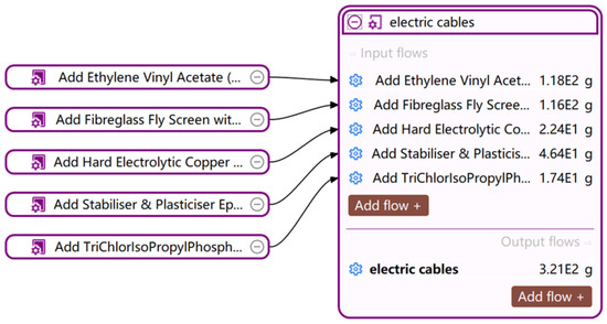
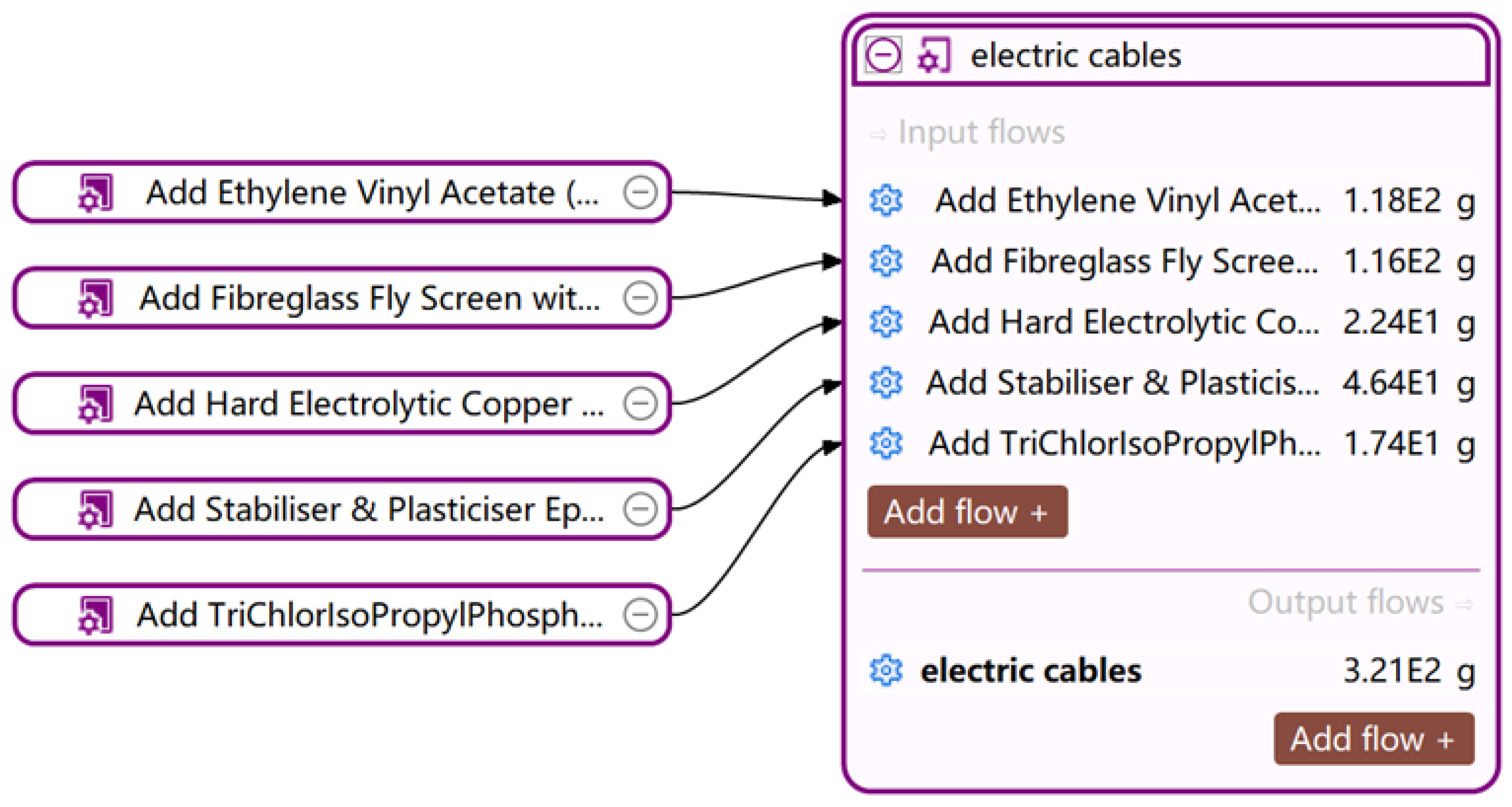
To evaluate the effectiveness of our proposed carbon footprint uncertainty quantification method, we compare its results with those obtained using the standard approach and the traditional Monte Carlo simulation. We conduct comparative experiments on three representative products under an identical system boundary: a cable, a corrugated tube, and a heating pad. As a representative case, the cable product comprises Ethylene Vinyl Acetate (EVA) resin, fibreglass fly screen with DINP-plasticised polyvinyl chloride (SPVC) bead, hard electrolytic copper wire or drawn Section (100% PCR) (COPPER), stabiliser and plasticiser epoxidised soybean oil (ESBO), and trichloroisopropyl phosphate (TCP/TTCP). For the corrugated tube and heating pad, the life-cycle inventories were constructed from their respective bills of materials and processed using the same modeling procedure. Figure 2 illustrates the material-flow model for the cable as a representative example; the corrugated tube and heating pad are modeled using the same system boundary and workflow. The comparison results for all three products are summarized in Table 2.

Figure 2. Material Flow Demonstration for Carbon Footprint Assessment of Cable Products.

Table 2. Comparison results of different methods.

Method	Cable	Corrugated Tube	Heating Pad
Standard method	0.962	0.793	1.385
Monte Carlo simulation	0.995	0.827	1.424
Ours	1.002	0.841	1.475

Across the three products, the carbon footprint estimated by the proposed method is slightly higher than the estimates produced by the other two algorithms (e.g., cable: 1.002 compared with 0.962 and 0.995; corrugated tube: 0.841 compared with 0.793 and 0.827; heating pad: 1.475 compared with 1.385 and 1.424). Moreover, the proposed method exhibits higher sensitivity and more effectively captures uncertainty propagation under boundary constraints. Compared with conventional Monte Carlo simulations, the proposed method yields a more continuous representation of the parameter space. By emphasizing high-confidence intervals while suppressing noise in the distribution tails, the proposed method produces more stable estimates.

3.2. Analysis of the Improved Mechanism for Uncertainty Expression

Traditional methods mainly rely on point estimation or a single probability distribution to describe uncertainty. They have several limitations: (1) Input-data fuzziness is not explicitly modeled; (2) structural differences among parameters are reduced to a single random perturbation; and (3) the uncertainty propagation pathway is not hierarchically differentiated.

The method proposed in this paper systematically improves the process in four logical stages:

• Since the traditional approaches often rely on averaged parameter values, they overlook heterogeneity across data sources. Our proposed algorithm incorporates an LLM-based evidence distillation module that uses four indicators to rule weights. These indicators quantify source-level credibility, including source authority, timeliness, consistency, and quality score. Consequently, each parameter is represented not as a single point estimate but as a credibility-weighted fuzzy set, which serves as the first layer of uncertainty representation.
• Conflict Resolution among Multi-Source Rules: In cases of conflicting multi-source rules, traditional methods struggle to integrate mutually exclusive information. We utilize a weighted Max–Min operator and apply a nonlinear envelope to the membership functions of high-credibility rules. This operation enables the collaborative fusion of multiple pieces of evidence, maintaining weight differences among rules and ensuring that the output possibility distribution reflects the cumulative effects of both knowledge uncertainty and data uncertainty. This step lays the foundation for subsequent probability mapping.
• Mapping Fuzzy Possibility Intervals: We map fuzzy possibility intervals into a sampleable truncated normal distribution using the maximum entropy principle. The global parameter physical boundaries are determined within the range [A, B], while the scenario interval [L, H] represents the high-confidence working interval. This dual-layer mapping mechanism ensures distribution continuity while avoiding the amplification effect of extreme values in Monte Carlo sampling. As a result, it significantly improves the stability and controllability of the simulation.
• Three-Scenario Monte Carlo Simulation and Uncertainty Synthesis: In contrast to traditional Monte Carlo methods, which only consider input randomness, our method distinguishes structural differences in parameter values by dividing the scenarios into low, medium, and high. Each scenario acquires local statistical features through conditional truncated sampling. The global mean and total variance are synthesized using fuzzy weighting. Table 3 presents the uncertainty decomposition for both traditional Monte Carlo and the three-scenario simulation.

Table 3. Decomposition and robustness diagnostics of uncertainty.

Method	Mean	SD	5%CI	95%CI	Normalised Weight
Traditional MC	0.995	0.058	0.913	1.105	—
Scenario: Low	0.994	0.050	0.910	1.071	0.127
Scenario: Mid	1.003	0.052	0.916	1.079	0.760
Scenario: High	1.010	0.048	0.922	1.086	0.113
Variance decomposition (Ours)
Total variance $\mathrm{Var}\left(\widehat{Y}\right)$					$2.54\times {10}^{-3}$
Intra-scenario variance ${\sum }_i{\omega }_i{s}_i^2$					$2.5367\times {10}^{-3}$
Inter-scenario variance ${\sum }_i{\omega }_i{({\overline{y}}_i-\widehat{y})}^2$					$2.50\times {10}^{-7}$
Inter-scenario share ${\mathrm{Var}}_{\mathrm{inter}}/\mathrm{Var}\left(\widehat{Y}\right)$					≈0.01%

Table 3 shows that the inter-scenario component accounts for a negligible fraction of the total variance, indicating that overall uncertainty is not primarily driven by the low/medium/high linguistic split but instead is dominated by within-scenario variability. In addition, the three scenario means are similar, and the mid scenario carries the dominant weight, suggesting that the ternary fuzzy design does not introduce exaggerated structural separation. Because common random numbers and equal sample sizes are used across scenarios, the remaining differences can be attributed to the rule-constrained intervals rather than to incidental sampling noise. Regarding Monte Carlo stability, the reported confidence intervals quantify sampling variability at the chosen computational budget, and the corresponding uncertainty in the estimated mean scales as $\mathrm{SD}/\sqrt{N}$.

3.3. Analysis of Result Robustness and Uncertainty Interpretability

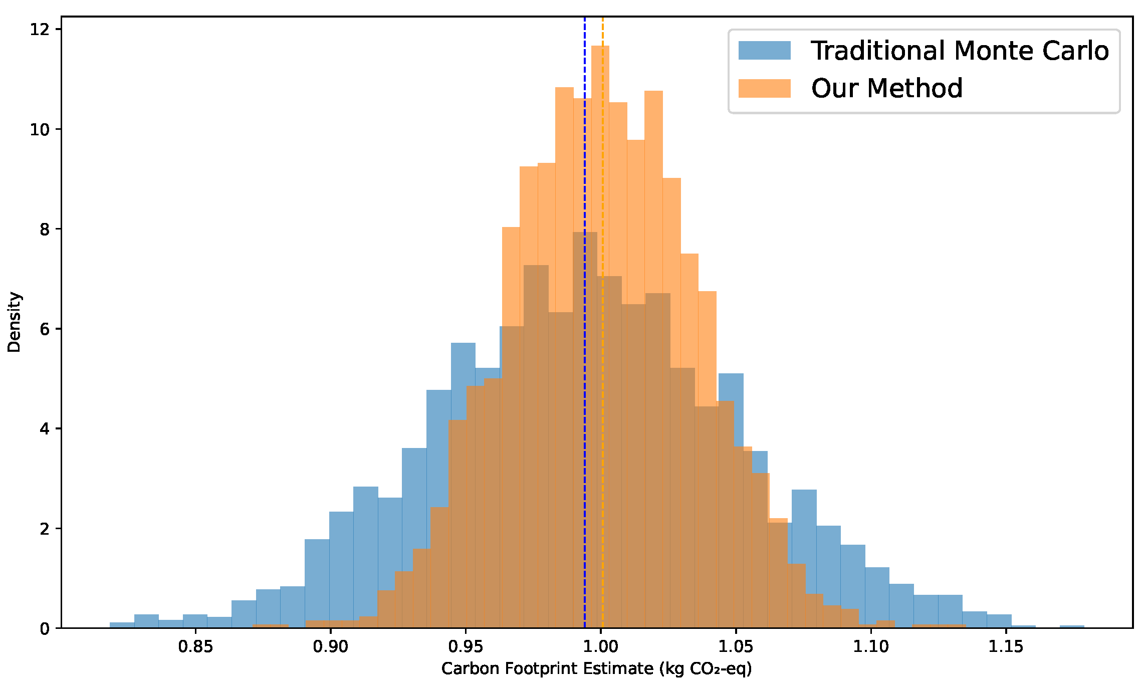
Figure 3 compares the output distributions produced by the traditional Monte Carlo method and the proposed method. The blue histogram and dashed line represent the traditional Monte Carlo method and its corresponding mean, respectively, whereas the orange histogram represents the proposed method and its corresponding mean. Figure 3 also shows the relative dispersion and central tendency of the carbon footprint estimates under both approaches. The proposed method yields a more concentrated distribution, characterized by a narrower spread around a similar mean. In contrast, the traditional Monte Carlo method exhibits a broader spread. For the same number of simulations, these results indicate that the proposed approach reduces uncertainty. The proposed method demonstrates the following performance characteristics:

Figure 3. Density-normalized histograms of the output distributions.

More Stable Result Distribution: In repeated simulations, the output variance of the proposed method is significantly lower than that of the traditional Monte Carlo method, indicating greater robustness. Even when parameters are incomplete or the sample distribution is skewed, the truncated normal background ensures that sampled values stay within a reasonable range, preventing outlier samples from amplifying the results.

Clear and Traceable Sources of Uncertainty: Unlike traditional methods, which combine all input uncertainties into a single variance, our method retains two distinct components during the weighted synthesis: intra-scenario variance and inter-scenario variance. The former accounts for the random uncertainty caused by input fluctuations, while the latter reflects model uncertainty due to structural differences in parameter intervals.

Higher Robustness to Extreme Samples: In traditional Monte Carlo simulations, extreme parameters (e.g., high-emission data exceeding the 99th percentile) can significantly skew the mean result. In contrast, the proposed method limits the sampling range through the upper and lower boundaries [A, B] of the truncated normal distribution, ensuring stable results across multiple simulation rounds.

Such high-precision traceability is distinctively valuable for meeting the transparent reporting standards of SDG 9 (Industry) and SDG 12 (Responsible Production). Furthermore, by rigorously distinguishing genuine emission reductions from statistical noise, the proposed framework provides the validated evidence base required for the Science Based Targets initiative (SBTi) and corporate net-zero pathways, directly supporting the climate action goals of SDG 13. In practical corporate carbon management, the uncertainty ranges and scenario-weighted outputs can be used to screen sourcing alternatives by assessing whether candidate options are distinguishable beyond uncertainty, while the uncertainty attribution and scenario decomposition help prioritize process improvements and data collection where uncertainty is decision-critical, and support the sequencing of decarbonization investments by distinguishing within-scenario variability from between-scenario structural differences.

3.4. Expert Traceability Audit

To ensure this credibility assessment remains transparent and auditable at scale, particularly for rules automatically extracted by LLMs, we further operationalize traceability by logging a provenance record for every extracted rule $R_i$ (Equation (1)) and its evidence weight $w_i$ (Equation (2)). We conducted a focused expert audit to assess the traceability and evidential grounding of the LLM-extracted rule base. Two domain experts independently reviewed a random sample of $K=30$ rules. For each rule, the experts evaluated three binary criteria: (C1) Evidence support, whether the cited evidence supports the factor definition and extracted numerical interval(s); (C2) Extraction correctness, whether the extracted fields (factor, units, interval bounds, and antecedent qualifiers) are consistent with the evidence; and (C3) Weight plausibility, whether the resulting $w_i$ is directionally consistent with the source metadata and the credibility dimensions in Equation (2). A rule is marked as Pass only when all three criteria are satisfied.

The overall audit outcomes, inter-expert agreement, and field-level agreement between the LLM-extracted fields and expert annotations are summarised in Table 4. For reproducibility, interval agreement is evaluated using intersection-over-union, defined for $I=[l,h]$ and $I^{*}=[l^{*},h^{*}]$ as $\mathrm{IoU}(I,I^{*})={\displaystyle \frac{|I\cap I^{*}|}{|I\cup I^{*}|}}$, with a match counted when $\mathrm{IoU}\ge 0.7$. Representative audited records are reported in Table 5, illustrating how each rule can be inspected via its provenance record and weight decomposition. The flagged cases primarily stem from incomplete or overly broad antecedent qualifiers, occasional unit or field mismatches, and discrepancies in the estimated $S_{\mathrm{cons}}$, as categorised in the audit tables.

Table 4. Summary of the expert traceability audit.

Metric	Value
Audited rules (K)	30
Experts	2
Sampling scheme	Simple random sampling from the rule base
Pass rate (C1–C3 all Pass)	86.7% (26/30); 95% CI: [70.3%, 94.7%]
Fail rate (at least one of C1–C3 fails)	13.3% (4/30); 95% CI: [5.3%, 29.7%]
Inter-expert agreement (Cohen’s $\kappa$)	0.81
Factor match vs. expert extraction	93.3% (28/30); 95% CI: [78.7%, 98.2%]
Factor mismatch rate	6.7% (2/30); 95% CI: [1.8%, 21.3%]
Interval agreement (IoU $\ge 0.7$)	83.3% (25/30); 95% CI: [66.4%, 92.7%]
Interval mismatch rate (IoU $<0.7$)	16.7% (5/30); 95% CI: [7.3%, 33.6%]

Table 5. Representative provenance records and expert audit outcomes.

RuleID	EvidenceID	Source	${\mathit{S}}_{\mathbf{src}}$	Time	${\mathit{S}}_{\mathbf{cons}}$	${\mathit{S}}_{\mathbf{quality}}$	${\mathit{w}}_{\mathit{i}}$	Expert1	Expert2
R-01	EVID-0142	Paper	0.90	0.83	0.80	0.85	0.51	P/P/P	P/P/P
R-02	EVID-0038	Report	0.70	0.62	0.75	0.65	0.21	P/P/P	P/P/P
R-03	EVID-0201	Internal	0.80	0.93	0.70	0.70	0.36	P/P/P	P/P/P
R-04	EVID-0114	Report	0.70	0.58	0.60	0.60	0.15	P/F/P	P/F/P
R-05	EVID-0079	Web	0.40	0.74	0.55	0.45	0.07	F/F/P	F/P/P

Note: Time denotes the timeliness component (e.g., $e^{-\lambda ·ag{e}_i}$). P/F = Pass/Fail.

3.5. Contribution Analysis of Typical Environmental Impacts

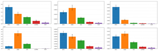
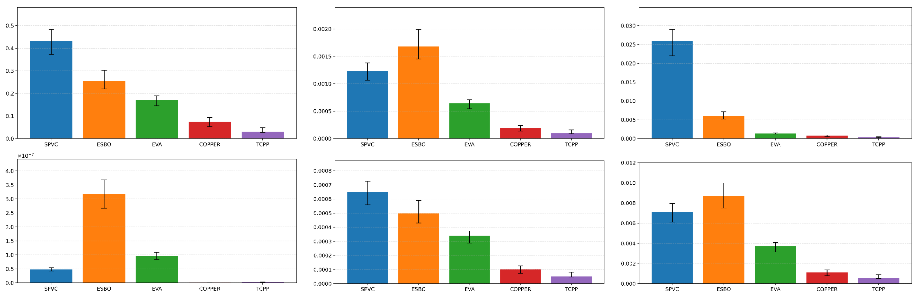
Based on the experimental data, the uncertainty contributions of various component factors to different environmental impacts are further identified, as shown in Figure 4.

Figure 4. Material-level contribution analysis results computed in openLCA for six impact categories. Bars represent the average contribution of each material/component across Monte Carlo runs, and error bars indicate the uncertainty dispersion obtained from the Monte Carlo simulation.

Figure 4 presents the material-level contribution results calculated in openLCA under Monte Carlo simulation. The bars summarize the contributions of each material/component, and the error bars reflect the variability of these contributions across Monte Carlo runs. Overall, SPVC and ESBO dominate most impact categories. In climate change (GWP100), SPVC shows the largest contribution, indicating that upstream processes associated with SPVC are the main drivers of greenhouse-gas-related impacts in the inventory. For freshwater and terrestrial acidification, SPVC and ESBO remain the primary contributors, consistent with emission profiles commonly associated with chemical production in their supply chains. In freshwater ecotoxicity, SPVC exhibits the highest contribution, suggesting a stronger association with toxicity-related emissions along its life cycle. For eutrophication-related categories, ESBO is the leading contributor in freshwater eutrophication, while SPVC and ESBO both contribute substantially in marine and terrestrial eutrophication, indicating that nutrient-related emissions in their upstream processes can be important drivers of these impacts. Importantly, the uncertainty ranges shown by the error bars provide an uncertainty-aware view of the contribution ranking: where ranges overlap, the relative ranking should be interpreted with caution, whereas clearer separation supports the robustness of the identified dominant contributors.

In summary, SPVC and ESBO consistently contribute the most across multiple categories, particularly climate change, freshwater ecotoxicity, acidification, and eutrophication. By contrast, copper wire shows comparatively smaller contributions in climate change and ecotoxicity, with impacts mainly driven by energy use during production. EVA contributes modestly to climate change and eutrophication, while still contributing to other categories to a lesser extent.

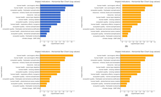
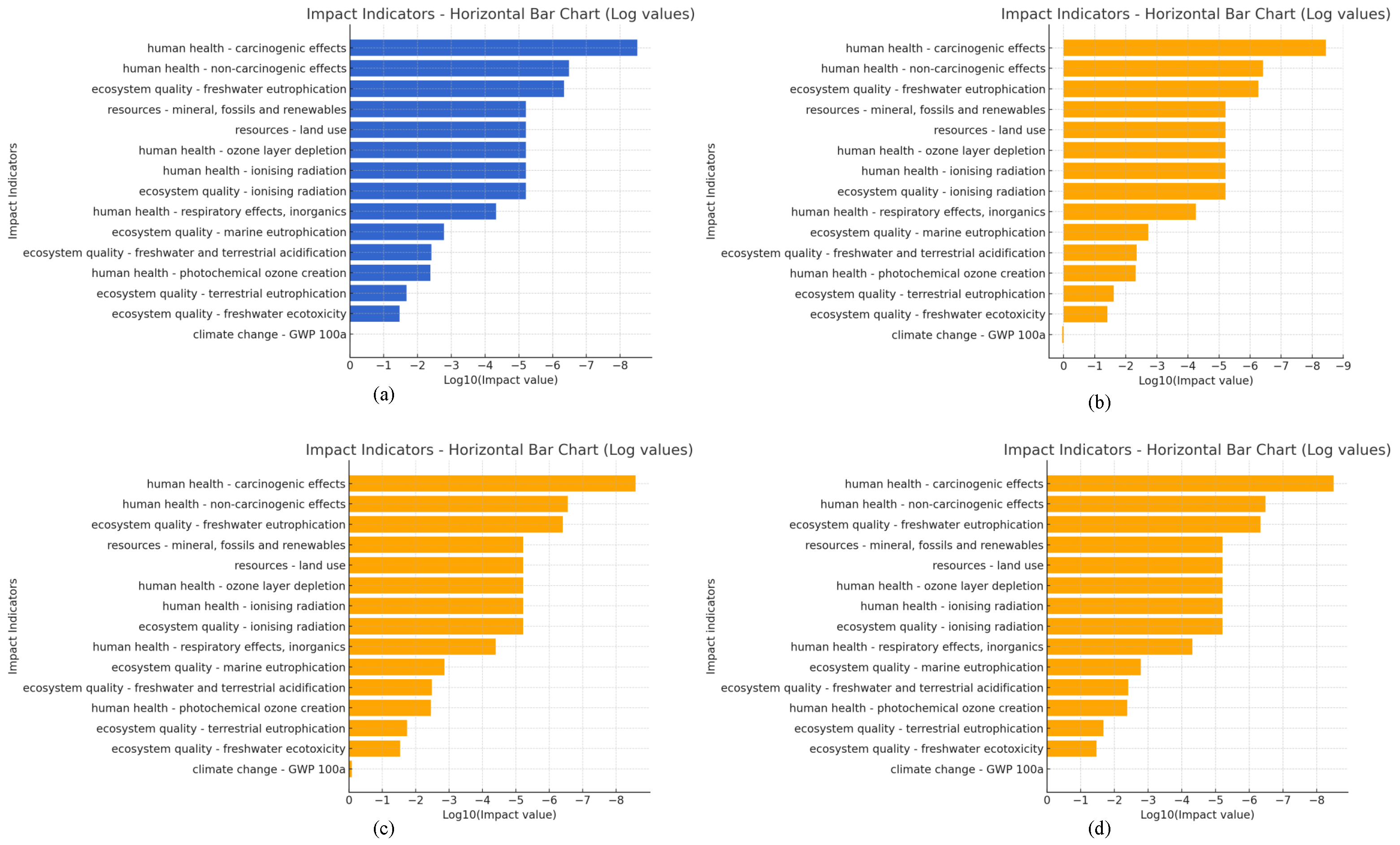
Concurrently, the environmental impacts of products within the same system boundary across different categories were calculated, and the results are presented in Table 6. After applying a logarithmic transformation to the data, these results are shown in Figure 5.

Table 6. Environmental Impact Results Table.

Impact Category	Conventional Method	High Scenario	Mid Scenario	Low Scenario
climate change: GWP 100a/kg CO2-Eq	−0.0168	0.04708	−0.01518	−0.08787
ecosystem quality: freshwater ecotoxicity/CTU h·m3·yr	−1.46585	−1.40994	−1.46674	−1.53224
ecosystem quality: terrestrial eutrophication/mol N-Eq	−1.6751	−1.60977	−1.67182	−1.74449
human health: photochemical ozone creation/kg ethylene-Eq	−2.38195	−2.31876	−2.38091	−2.45223
ecosystem quality: freshwater and terrestrial acidification/mol H+-Eq	−2.41454	−2.34872	−2.41117	−2.48413
ecosystem quality: marine eutrophication/kg N-Eq	−2.78516	−2.72354	−2.78516	−2.85699
human health: respiratory effects, inorganics/kg PM2.5-Eq	−4.32343	−4.25603	−4.31857	−4.39165
ecosystem quality: ionising radiation/mol N-Eq	−5.21153	−5.21153	−5.21153	−5.21153
human health: ionising radiation/U235-Eq	−5.21153	−5.21153	−5.21153	−5.21153
human health: ozone layer depletion/CFC-11-Eq	−5.21153	−5.21153	−5.21153	−5.21153
resources: land use/kg Soil Organic Carbon	−5.21153	−5.21153	−5.21153	−5.21153
resources: mineral, fossils and renewables/kg Sb-Eq	−5.21153	−5.21153	−5.21153	−5.21153
ecosystem quality: freshwater eutrophication/kg P-Eq	−6.3364	−6.27159	−6.33231	−6.40293
human health: non-carcinogenic effects/CTUh	−6.48273	−6.41416	−6.47913	−6.55557
human health: carcinogenic effects/CTUh	−8.50463	−8.43665	−8.5011	−8.57682

Figure 5. Comparison of environmental impact outcomes across different categories: (a) conventional calculation method; (b) high-scenario result from the three-scenario Monte Carlo simulation; (c) medium-scenario result from the three-scenario Monte Carlo simulation; (d) low-scenario result from the three-scenario Monte Carlo simulation.

Figure 5a illustrates the conventional calculation method, while Figure 5b–d represent the high, medium, and low scenarios of the three-scenario Monte Carlo simulation. In the climate change-GWP 100a category, the results from the three-scenario simulation present and analyse the total carbon emissions across multiple tiers. Compared with the conventional method, our method highlights the rationality of the weighting distribution across the high, medium, and low intervals.

As shown in Figure 5, different types of environmental impacts vary significantly. Larger values (logarithmic values close to 0) represent impacts that are more significant to the environment, ecology, or health, while smaller values (logarithmic values close to −12) indicate lesser impacts.

4. Limitations and Future Works

Despite the promising performance of our proposed framework, several limitations warrant discussion. Although we expanded the demonstrations to multiple products, the case study was conducted under largely consistent system boundaries and relied on similar data sources. Therefore, the results should be interpreted as methodological evidence supporting transparent uncertainty quantification and attribution, rather than as universally generalizable conclusions for sustainable decision-making across heterogeneous contexts. Methodologically, we adopt a truncated normal distribution for probabilistic mapping and partition the extracted interval into three sub-intervals; this design may be less suitable for strongly non-Gaussian or multimodal parameter regimes and could be extended in future work by incorporating more flexible distributional assumptions and adaptive partitioning. In addition, the current implementation remains a prototype, and further engineering efforts are required for practical deployment, including robust data pipelines, user-centered interfaces, and integration with existing LCA tools.

5. Conclusions

To address ambiguity in input data and limited transparency in carbon footprint assessment, this study proposes a truncated-normal and fuzzy-weighting uncertainty quantification framework. The framework integrates LLM-based evidence distillation, credibility-aware fuzzy inference, and probabilistic propagation, enabling linguistic and multi-source evidence to be mapped into physically constrained, sampleable probability models for Monte Carlo analysis. In the case study, our approach produces more stable and robust results than conventional methods. It improves interpretability by separating within-scenario random variability from between-scenario structural uncertainty. Overall, we provide a traceable and decision-relevant tool for risk-aware carbon footprint reporting and uncertainty management in manufacturing applications.

References

- de Bortoli, A.; Bjørn, A.; Saunier, F.; Margni, M. Planning sustainable carbon neutrality pathways: Accounting challenges experienced by organizations and solutions from industrial ecology. Int. J. Life Cycle Assess. 2023, 28, 746–770. [Google Scholar] [CrossRef] [Scilit]
- Kaur, R.; Patsavellas, J.; Haddad, Y.; Salonitis, K. Carbon accounting management in complex manufacturing supply chains: A structured framework approach. Procedia CIRP 2022, 107, 869–875. [Google Scholar] [CrossRef] [Scilit]
- He, Q.; Wu, X.; Ding, X. Uncertainty in the Carbon Footprint accounting and evaluation of textile and apparel products: A systematic review. J. Clean. Prod. 2025, 492, 144885. [Google Scholar] [CrossRef] [Scilit]
- Xu, X.; Cao, X.; Yu, L. Carbon emissions forecasting based on tensor decomposition with multi-source data fusion. Inf. Sci. 2024, 681, 121235. [Google Scholar] [CrossRef] [Scilit]
- Sun, X.; Pan, X.; Jin, C.; Li, Y.; Xu, Q.; Zhang, D.; Li, H. Life Cycle Assessment-Based Carbon Footprint Accounting Model and Analysis for Integrated Energy Stations in China. Int. J. Environ. Res. Public Health 2022, 19, 16451. [Google Scholar] [CrossRef] [Scilit]
- Sizirici, B.; Fseha, Y.; Cho, C.S.; Yildiz, I.; Byon, Y.J. A Review of Carbon Footprint Reduction in Construction Industry, from Design to Operation. Materials 2021, 14, 94. [Google Scholar] [CrossRef] [Scilit] [PubMed]
- Bailis, R.; Drigo, R.; Ghilardi, A.; Masera, O. The carbon footprint of traditional woodfuels. Nat. Clim. Change 2015, 5, 266–272. [Google Scholar] [CrossRef] [Scilit]
- Lenzen, M.; Sun, Y.Y.; Faturay, F.; Ting, Y.P.; Geschke, A.; Malik, A. The carbon footprint of global tourism. Nat. Clim. Change 2018, 8, 522–528. [Google Scholar] [CrossRef] [Scilit]
- Han, J.; Tan, Z.; Chen, M.; Zhao, L.; Yang, L.; Chen, S. Carbon Footprint Research Based on Input–Output Model—A Global Scientometric Visualization Analysis. Int. J. Environ. Res. Public Health 2022, 19, 11343. [Google Scholar] [CrossRef] [Scilit]
- Lenzen, M.; Wood, R.; Wiedmann, T. Uncertainty Analysis For Multi-Region Input-Output Models—A Case Study of the UK’s Carbon Footprint. Econ. Syst. Res. 2010, 22, 43–63. [Google Scholar] [CrossRef] [Scilit]
- Wang, Z.; Li, Y.; Cai, H.; Wang, B. Comparative analysis of regional carbon emissions accounting methods in China: Production-based versus consumption-based principles. J. Clean. Prod. 2018, 194, 12–22. [Google Scholar] [CrossRef] [Scilit]
- Adhikari, N.; Li, H.; Gopalakrishnan, B. A bibliometric and systematic review of carbon footprint tracking in Cross-Sector industries: Emerging tools and technologies. Sustainability 2025, 17, 4205. [Google Scholar] [CrossRef] [Scilit]
- Schulte, S.; Jakobs, A.; Pauliuk, S. Estimating the uncertainty of the greenhouse gas emission accounts in global multi-regional input–output analysis. Earth Syst. Sci. Data 2024, 16, 2669–2700. [Google Scholar] [CrossRef] [Scilit]
- Michiels, F.; Geeraerd, A. Two-dimensional Monte Carlo simulations in LCA: An innovative approach to guide the choice for the environmentally preferable option. Int. J. Life Cycle Assess. 2022, 27, 505–523. [Google Scholar] [CrossRef] [Scilit]
- Lee, K.M.; Lee, M.H.; Lee, J.S.; Lee, J.Y. Uncertainty Analysis of Greenhouse Gas (GHG) Emissions Simulated by the Parametric Monte Carlo Simulation and Nonparametric Bootstrap Method. Energies 2020, 13, 4965. [Google Scholar] [CrossRef] [Scilit]
- Yakut Şevik, S.E.; Şahin, A.D. Quantifying Sectoral Carbon Footprints in Türkiye’s Largest Metropolitan Cities: A Monte Carlo Simulation Approach. Sustainability 2024, 16, 1730. [Google Scholar] [CrossRef] [Scilit]
- He, B.; Pan, Q.; Deng, Z. Product carbon footprint for product life cycle under uncertainty. J. Clean. Prod. 2018, 187, 459–472. [Google Scholar] [CrossRef] [Scilit]
- Weyand, A.; Bausch, P.; Engel, B.; Metternich, J.; Weigold, M. Analysis of Uncertainty Factors in Part-Specific Greenhouse Gas Accounting. Sustainability 2023, 15, 16871. [Google Scholar] [CrossRef] [Scilit]
- Lee, K.; Ko, J.; Jung, S. Quantifying uncertainty in carbon emission estimation: Metrics and methodologies. J. Clean. Prod. 2024, 452, 142141. [Google Scholar] [CrossRef] [Scilit]
- Metropolis, N.; Ulam, S. The Monte Carlo Method. J. Am. Stat. Assoc. 1949, 44, 335–341. [Google Scholar] [CrossRef]
- Lancaster, H.O. The characterisation of the normal distribution. J. Aust. Math. Soc. 1960, 1, 368–383. [Google Scholar] [CrossRef] [Scilit]
- Benhamou, E.; Guez, B.; Paris, N. Three remarkable properties of the Normal distribution. arXiv 2018, arXiv:1810.01768. [Google Scholar] [CrossRef] [Scilit]
- Lloyd, S.M.; Ries, R. Characterizing, propagating, and analyzing uncertainty in life-cycle assessment: A survey of quantitative approaches. J. Ind. Ecol. 2007, 11, 161–179. [Google Scholar] [CrossRef] [Scilit]
- Tan, R.R. Using fuzzy numbers to propagate uncertainty in matrix-based LCI. Int. J. Life Cycle Assess. 2008, 13, 585–592. [Google Scholar] [CrossRef] [Scilit]
- Dubois, D.; Foulloy, L.; Mauris, G.; Prade, H. Probability-possibility transformations, triangular fuzzy sets, and probabilistic inequalities. Reliab. Comput. 2004, 10, 273–297. [Google Scholar] [CrossRef] [Scilit]
- Touvron, H.; Martin, L.; Stone, K.; Albert, P.; Almahairi, A.; Babaei, Y.; Bashlykov, N.; Batra, S.; Bhargava, P.; Bhosale, S.; et al. Llama 2: Open Foundation and Fine-Tuned Chat Models. arXiv 2023, arXiv:2307.09288. [Google Scholar] [CrossRef] [Scilit]
Disclaimer/Publisher’s Note: The statements, opinions and data contained in all publications are solely those of the individual author(s) and contributor(s) and not of MDPI and/or the editor(s). MDPI and/or the editor(s) disclaim responsibility for any injury to people or property resulting from any ideas, methods, instructions or products referred to in the content. |
© 2026 by the authors. Licensee MDPI, Basel, Switzerland. This article is an open access article distributed under the terms and conditions of the Creative Commons Attribution (CC BY) license.