


Abstract
Ontology-based risk assessment usually infers what a query needs before the query is posed. For a material the knowledge graph does not contain, or when a query changes how similarity is measured, part of that information depends on the query itself. We propose an on-demand cycle that, when a query names a material, computes its hazard-profile similarity to known materials from GHS hazard statements, injects the result into the knowledge graph as validated individuals, and retrieves consequence types ranked by lift. Similarities among materials already in the graph can be precomputed, so the cycle serves chiefly materials outside it. On 12,274 accidents from five databases, the cycle ran end to end for chlorine, benzene, and germane, a material absent from the graph, in about 7 s per query. In leave-one-out validation over 1933 accident–material cases, a recorded consequence type was among the top three in 63.5% of cases, against 47.0% with random target materials, and in 72.9% of the cases missed by a most-frequent-type baseline, against 60.1%. The gain varied by consequence type and material group and awaits confirmation on independent data. Because it computes from GHS hazard classifications, on which chemical regulations also rely, the cycle points toward dynamic assessment that could support chemical safety management.
1. Introduction
1.1. Background
Risk assessment in the process industries follows two broad lines [1]. One anticipates what may go wrong before an accident occurs [2,3]. The other records those findings so they can later be reviewed, reused, and revised [4]. Ontologies have served the second line, organising safety knowledge for reuse. They move what safety research has learned out of documents meant only for human readers and into a form a computer can act on. Materials, accidents, their consequences, and the relations among them are cast as a knowledge graph of classes and relations [5,6,7], and prediction follows those relations to find the accidents and consequences a material may lead to [8].
This works well for well-characterised hazards, where the materials, the equipment, and the accident record are all known, so the information a prediction needs can be prepared ahead of time. Newly introduced hazards are another matter [9,10]. Their accident records are thin, their operating conditions differ from one installation to the next and shift over time, and a prediction prepared for one configuration does not carry over to another. Where systematic prediction is needed most, the data it rests on are scarcest.
This is where the ontology approach meets a structural limit. Conventional methods infer everything in advance and write it into the knowledge graph, leaving a later query to read off the answer. That arrangement assumes that the objects a query may name are known when the graph is filled. For newly introduced hazards, the assumption is weaker, because the materials, installations, and conditions that will need assessment are settled as facilities are designed, built, and expanded, rather than when the ontology is built. The present study takes up one part of this problem, the material dimension. Operating conditions, release scenarios, and installation geometry lie outside its scope.
Where the record is too thin to answer directly, prediction has to fall back on comparing the material at hand with others that do have accidents on record. For materials already in the knowledge graph, such comparisons can be computed and stored ahead of time. For a material the graph does not yet contain, the comparison can be formed only once a query supplies a description of the material, and the same holds when a query changes how similarity is defined, for example by weighting the codes differently. Part of what a prediction needs is then settled when the query arrives.
1.2. Related Work
Work related to this study falls into three strands.
The first applies ontologies to safety and reliability analysis, moving the knowledge such analysis produces into a machine-processable form [11,12,13] that can be reused across designs or fed into automated analysis [8,14]. Representing an accident as a causal chain of cause, deviation, and consequence [15,16] and deriving scenarios along that chain [17,18,19] is, in form, the same traversal used here, which runs from a material to its accidents and on to consequence types.
The second is ontology-based data access (OBDA). It concerns how a query written in an ontology’s vocabulary can be answered against data held elsewhere [20,21], and it has long been debated whether the required values should be computed before a query or handled when it arrives [22,23]. Mappings in OBDA and virtual knowledge graph systems are not limited to copying stored values. They can apply SQL expressions or registered functions to source data, so derived values can also be produced when a query is answered [24,25,26,27].
The third infers from similar materials when data are scarce. Read-across, familiar in regulatory toxicology, is the representative case. It predicts a target material’s properties from those of materials judged similar enough [28,29,30,31]. This line of work keeps the prediction itself separate from how reliable it is, and has shown that the usefulness of a similarity measure depends on what is being predicted.
This study stands at the meeting point of the three. Ontology-based safety research embeds its inference before a query arrives, while this study computes at query time the values that depend on the material the query names. OBDA computes or retrieves values from a fixed set of data sources through mappings written in advance. Here the input of the computation, the hazard-code profile of the queried material, may come from the query itself rather than from any source, and the result is added to the working knowledge graph as individuals that can be validated and traversed. Section 2.4 develops this comparison. Read-across is usually run as a separate analysis over a chemical dataset, and this study carries out a similarity inference of the same kind inside the ontology at query time. The problem addressed is how to use, within an ontology, values whose inputs become available only when a query is posed.
1.3. Proposed Approach and Contributions
We propose an on-demand computation-injection architecture. When a query names a material, the architecture runs through four stages. It computes the value the query has just made determinate, namely the material’s similarity to the others in the knowledge graph over their GHS codes. It injects that similarity as a relation that can be traversed. It validates the injected content. And it retrieves the prediction along the newly connected relations. The reasoner takes part only in validation and plays no part in the prediction, which comes from aggregating the computed values along relations, with no rules involved.
The architecture resembles OBDA in deferring work to query time, and the resemblance deserves a precise statement. OBDA lets data spread across sources be queried through one ontology vocabulary. The data stay where they are, and an incoming query is rewritten into queries the sources can answer. Mappings can compute derived values from the source data, so the difference does not lie in whether computation takes place. It lies in where the input comes from and where the result is kept. An OBDA mapping computes over the tuples of the sources it was written for. The present cycle computes over an input supplied by the query, the hazard-code profile of the named material, which need not appear in any source, and it asserts the result into the working graph as individuals that are validated before retrieval. For materials already present in the data, the same similarities could be precomputed or produced by a suitable mapping, and Section 2.4 treats that case explicitly.
The study makes three contributions. The first is the on-demand cycle itself, formulated as four stages of computation, injection, validation of the injected content, and retrieval. It brings query-dependent values within reach of the ontology at query time, with no rules and no parameters fitted to the data. The second is a delimitation of when the cycle is needed. For materials already in the knowledge graph, precomputing all pairwise similarities, or a hybrid that precomputes them and computes only what a new material requires, is a valid alternative. The cycle becomes necessary for a material the graph does not contain, and for a similarity definition chosen only at query time. The third is a validation on chemical accident data along three lines. It confirms that prediction runs end to end, including for a material absent from the knowledge graph. It measures, stage by stage, the one-time and per-query costs of computing on demand and of precomputing. And it compares the predictions with recorded outcomes by withholding accidents one at a time and, in a stricter variant, every accident of the target material.
That third line calls for care in how performance is measured. Overall hit rate turns out to be a poor yardstick, since it runs high even when no substance information is used, and only the most common consequence types are returned. We therefore also measure on the cases that returning the common types cannot answer, and we compare the architecture with baselines that use no substance information, including one that keeps the ranking rule but assigns the target material at random. Dividing the results by consequence type then indicates for which types hazard-profile similarity carries information in this dataset.
The study was prompted by new energy infrastructure such as high-pressure hydrogen pipelines, whose accident history is still thin. The present work does not model pipelines, operating conditions, or hydrogen-specific accidents, and it makes no claim of applicability to them. It addresses the more general situation of predicting consequence types for a material whose own accident record is thin or absent. Section 4 returns to pipelines only as a possible future application.
2. Methodology
2.1. Accident Dataset and Hazard Codes
The accident records come from five databases. They are the National Toxic Substance Incidents Program of the Agency for Toxic Substances and Disease Registry in the United States (NTSIP) [32], the High Pressure Gas Accident Case Database of the High Pressure Gas Safety Institute of Japan (KHK) [33], the Major Accident Reporting System of the European Commission Joint Research Centre (eMARS) [34], the serious accident case records of the Korea Occupational Safety and Health Agency (KOSHA) [35], and the Central Reporting and Evaluation Office for Major Accidents of the German Environment Agency (ZEMA) [36]. The integrated set holds 12,274 accidents: 6296 from KHK (2000–2020), 3951 from NTSIP (2013–2014), 1175 from eMARS (1979–2022), 695 from KOSHA (2014–2022), and 157 from ZEMA (2011–2020). After the databases were merged, records suspected of describing the same accident in more than one source were flagged; each flagged pair was reviewed manually against the accident descriptions, dates, and outcomes, and records judged to describe the same accident were removed. A later check of the integrated set for accidents from different sources with the same date and the same set of materials found 38 remaining candidate groups. In the evaluation of Section 3.3, a candidate duplicate of the withheld accident entered the supporting data in 4 of the 1933 cases and in none of the R_blind region.
Every accident carries at least one consequence label. The labels of each source were mapped to a common vocabulary of seven consequence types, namely injury, fire, explosion, property damage, fatality, dispersion, and environmental damage, together with two labels that record no outcome, NoSignificantConsequence and Unknown. An accident may carry several types, and all of them are kept. Injury and fatality are assigned when the record reports at least one injured person or at least one death, and the labels agree with the recorded counts in every source. Fire, explosion, and dispersion are the event types recorded by eMARS, dispersion denoting a release of the substance to the surroundings, and Unknown is the label for an eMARS record whose event type is not given. Property damage and environmental damage are assigned when the source records material losses or harm to the environment. NoSignificantConsequence marks a record that reports no casualty and no damage, and it can occur together with an event type, for example in a dispersion without casualties. The mapping from the fields of each source is given in Supplementary Table S1. The sources differ in what they record. KHK, NTSIP, and ZEMA use only NoSignificantConsequence, injury, and fatality. Property damage and environmental damage appear in eMARS and KOSHA, and fire, explosion, dispersion, and Unknown appear only in eMARS (Supplementary Table S1). Results for these types therefore rest on the sources that record them.
Materials involved in each accident are linked to GHS hazard statements [37]. The records name 1825 distinct materials, of which 421 carry GHS hazard statement codes, and two of these are recorded only as “No hazard”. GHS hazard statements were attached to materials by CAS number when the records of the five databases were converted to a common format, using a single lookup, so that a CAS number carries the same statements in every source. Materials without a CAS number received no statements in that lookup. Statements were then retrieved from the GHS Classification section of PubChem [38], taking all hazard statements listed there, for 142 materials that had a CAS number but no statements in the lookup and for 7 materials without a CAS number that are involved in at least two accidents, identified by name in a search of 19 such materials. The remaining 272 materials, including the two recorded as “No hazard”, kept the statements from the lookup. Only these 421 materials enter the analysis. In all, 7866 accidents involve at least one of the 421 materials, and the other 4408 accidents enter neither the evaluation nor the supporting data. Fields that the method does not use, such as release quantities, do not affect whether a record is included, so their missing values need no treatment.
The evaluation uses accident–material cases. An accident involving several GHS-coded materials contributes one case per material. Accidents whose only labels are NoSignificantConsequence or Unknown carry no outcome to predict and are excluded from evaluation, as described in Section 2.3.4. This leaves 1933 cases from 1388 accidents. Cases carry 1.83 consequence types on average. The supporting data from which predictions are made are wider than the evaluation set. They include every accident of the materials selected as similar, including accidents whose only labels are NoSignificantConsequence or Unknown. Supplementary Figure S1 and Table S1 trace the records through each step.
2.2. Overall Architecture
Conventional ontology methods treat the ontology as a repository. It is completed and filled once, and a query reads the answer off it when it arrives. The present architecture works differently. When a query arrives, it computes the required value, injects it into the ontology, and predicts on that basis.
Two artefacts are loaded at start-up. One is the T-Box (Terminological Box), the conceptual scheme that defines the terms of the domain and the relations among them. The other is the A-Box (Assertional Box), the data that populate that scheme with actual instances. The A-Box in this study holds the accidents of Section 2.1 and the 421 materials classified under the GHS (Globally Harmonized System, the international scheme for classifying and labelling the hazards of chemical substances) [37], and comprises 183,710 triples, a triple being the basic unit of a knowledge graph that states a single fact in subject-relation-object form. Only three relations matter in this section, because the whole prediction path rests on them. The relation hasGHSCode links a material to the GHS hazard statement codes assigned to it, which are extracted individually with the pattern H\d{3}[dfi]?. The relation hasMaterial links an accident to the materials involved in it, and hasConsequence links an accident to the consequence types observed in it.
None of these three relations records how similar materials are to one another. Predicting the accidents of a material means comparing it with others, yet which materials are comparable, and how close they are, appears nowhere in the loaded knowledge graph. This similarity is the value the architecture computes, and it computes it once a query names a material.
Processing at runtime is therefore not a single pass over a finished knowledge graph but a cycle. Given a target material, the architecture runs four stages. It computes the similarity between the target and every material in the A-Box. It injects the computed pairs as entities the knowledge graph can hold. It validates the injected content. And it retrieves the prediction along the relation paths the injection has newly connected. Section 2.3 formalises the four stages.
Whether the on-demand cycle suits a case better than precomputation can be settled by a few questions, and the criteria proposed for OBDA in choosing between precomputing and handling at query time [23] rest on the same reasoning. The first question is whether what will be queried is fixed in advance. If it is not, there is no basis for choosing which values to precompute. The second is whether the values a query needs can be derived from what is already stored. The third is whether the required values depend on the query itself. Under these criteria, precomputation is adequate when queries name materials already in the graph and the similarity definition is fixed. The on-demand cycle is needed when the queried material lies outside the graph or when the similarity definition is chosen per query. How the costs of the two compare is a separate matter, taken up in Section 2.4.3 and Section 3.2.
2.3. The On-Demand Computation-Injection Cycle
The cycle is defined over a target material named by the query. Its four stages are described below in the order in which they run (Figure 1).
Figure 1.
The on-demand cycle in four stages. Stage 3 validates the injected content by an OWL-RL closure and SHACL shape checks on the injected module, and its entailments do not pass to the retrieval stage.
2.3.1. Stage 1: Compute
Each material is represented as a vector over the GHS codes it carries. Let the sorted set of all hazard statement codes extracted from hasGHSCode be the code vocabulary V, which has 71 codes in this dataset. Each material in the A-Box is then a vector over V, carrying 1 where the material has a code and 0 where it does not. Each vector is normalised to unit length, so that the product of two vectors is their cosine similarity [28,29]. A material without any valid code keeps a zero vector, has similarity 0 to every other material, and therefore selects no neighbours. Two of the 421 materials fall in this case, calcium carbonate and polypropylene glycol, the two recorded only as “No hazard”.
On binary vectors, cosine similarity reduces to the number of shared codes divided by the geometric mean of the two code counts, which is the Ochiai coefficient. It is thus a set-overlap measure of the same family as the Jaccard (Tanimoto) coefficient, which divides by the size of the union instead [29]. It is 1 when two code sets are identical and 0 when they share no codes. We refer to the result as hazard-profile similarity. It measures how far two materials share classified hazards, as summarised by their GHS statements. It does not measure physicochemical or structural similarity, and two materials with similar hazard profiles may differ in volatility, density, or reactivity.
Selecting the materials to compare with a target t is done in one matrix-vector product. Every material whose similarity reaches the threshold θ is selected and returned in order of decreasing similarity:
That is, among all materials other than the target, those whose cosine similarity to the target is at least 0.3 are selected and returned as a list pairing each material with its similarity. The threshold is a design choice, not a value fitted to the data. It was set when similarity-based selection was first implemented, before the evaluation of Section 3.3 was designed, and was not adjusted afterwards. For orientation, two materials with six codes each reach 0.33 when they share two. At this threshold, the median number of neighbours per evaluated target is 133 (interquartile range 75–187, maximum 275). None of the 349 evaluated target materials has fewer than five neighbours except the two materials without codes, which have none (Supplementary Table S3). Section 3.3.3 reports how the results change for θ between 0.1 and 0.7.
Computation is deferred at this point. The code vectors merely transcribe what hasGHSCode already holds and can be built once when the knowledge graph is loaded. The similarities are not stored. Of all pairwise similarities, only the row a query calls for is formed. For materials already in the A-Box, with the similarity definition fixed, the full matrix could instead be computed once and would then serve any θ, and Section 2.4.3 considers that option. For a target outside the A-Box, the row can be formed only after the query supplies its codes.
2.3.2. Stage 2: Inject
Stage 2 declares four new items in the ontology at runtime. They are a class MaterialSimilarity for the similarity relation between materials, two properties hasSubjectMaterial and hasSimilarMaterial for which material the relation runs from and to, and a property similarityScore for the value, typed as xsd:decimal. For each pair returned by Stage 1, one MaterialSimilarity individual is created, with the target as its subject material, the selected material as its similar material, and the similarity, rounded to four decimal places, as its value. A target outside the A-Box is first created as a material individual carrying the codes supplied by the query.
The injected individual turns the relation “similar to” between two materials into an object of its own. The relation is named, stood up as an individual, and given a numeric similarity, which lets the retrieval stage address and follow it. These individuals are not entailed by the T-Box and the loaded A-Box. No reasoning over the loaded graph derives them, because they are the output of a numerical computation rather than of inference. For materials in the A-Box, they could be computed and asserted in advance, which is Plan A in Section 2.4. The cycle asserts them only when a query needs them, and for whatever material the query names.
2.3.3. Stage 3: Validate the Injected Content
Stage 3 checks that the injected individuals are well-formed and do not contradict the ontology, and it rejects the injection if either of the two checks reports a violation. Both checks run on a validation module extracted from the current state rather than on the working graph. The module contains the T-Box, the declarations of the injected vocabulary, every triple whose subject is an injected individual, every triple whose subject is a resource that an injected individual refers to (one hop, no further), and all owl:sameAs and owl:differentFrom assertions of the graph. Accidental individuals and all other A-Box triples are left out unless they are one hop from an injected individual.
The first check is an OWL-RL closure of the module [39], during which every error the reasoner reports is collected, including rules that fire when an individual is asserted to be both the same as and different from another, or when an individual falls into two disjoint classes. So that these rules have something to act on, the injected vocabulary is declared with 25 runtime axiom triples. The three properties are declared functional with stated domains and ranges; similarity individuals are disjoint from materials and from accidents, materials are disjoint from accidents, and a property derived from the subject and similar material is irreflexive, so that a material cannot be declared similar to itself. The second check validates the injected individuals against SHACL shapes [40]. Each individual must have exactly one subject material and exactly one similar material; the two must differ, both must be materials, and the score must be a number between 0 and 1. The closure cannot express the counting and value-range conditions, which is why both checks are used. The axioms and shapes are listed in Supplementary Table S11.
The checks were tested by injecting ten kinds of deliberately malformed content, among them a score of 1.5, a missing subject material, two scores on one individual, an accident in place of a similar material, and a material declared similar to itself (Supplementary Table S11). All ten were rejected. The OWL-RL closure detected six of them, and the SHACL shapes all ten. Well-formed injections for chlorine, benzene, and germane were accepted. The verdicts on the module were the same as those obtained by running both checks over the whole graph, for all thirteen injections. This agreement was shown for these injections and is not a general proof. A contradiction that could be derived only through a chain of two or more steps beyond the injected individuals would fall outside the module.
Two properties of the stage are deliberate. Both checks run on a module extracted from the current state, so the working graph stays as it was and the retrieval stage reads only the injected values. And Stage 3 decides only whether an injection is accepted. The triples produced by the closure are discarded and take no part in the ranking. Stage 3 runs after every injection.
2.3.4. Stage 4: Retrieve
Stage 4 reads the injected individuals back and aggregates along two relations. Two indices, built when the knowledge graph is loaded, give, for each material, the accidents it was involved in and, for each accident, the consequence types observed in it. Joining the two yields a two-step path from material to accident to consequence type.
Two labels, NoSignificantConsequence and Unknown, are excluded from the candidate types and from the evaluation. Both are information-free labels. They record not that a particular outcome occurred but that no meaningful outcome was registered, or that the outcome was never confirmed. To credit a prediction of either would reward the mere repetition that no information is available. This exclusion fixes the evaluation set of Section 3 at 1933 cases from 1388 accidents, of which 207 cases from 147 accidents form the region where none of the three most frequent consequence types occur.
Given a target material t, Stage 4 collects every MaterialSimilarity individual whose subject material is t and, for each, retrieves the accidents its similar material was involved in. An accident is counted once even if several similar materials lead to it. Let the resulting set of supporting accidents be A_t, and let n(c) be the number of them in which consequence type c was observed. The observed rate of a consequence type is the proportion of the supporting accidents in which it occurs. This is compared with the base rate base(c), the proportion of the 12,274 accidents in which it occurs, and their ratio is taken as the lift [41]. Consequence types are ranked by decreasing lift:
The observed rate obs(c) is the proportion of supporting accidents in which c occurs, and lift is how many times greater this is than the proportion across the whole dataset. A lift above 1 means c occurred more often than usual in the accidents involving the similar materials. The ordering follows a fixed rule. Candidates are ranked by decreasing lift, then by decreasing observed rate, then by consequence-type name, so the order does not change from run to run. Because a single accident may show several consequence types, the observed rates do not sum to 1. Lift ranks consequence types by their relative enrichment among the supporting accidents. It is not an estimate of the probability that a type will occur, and a type can rank first with a lift below 1 when every type is under-represented.
One property of this rule, revisited in Section 3, is worth stating plainly here. Because base(c) enters as the denominator, a consequence type that is rare in the dataset attains a large lift even from a modest observed rate, so the magnitude of lift is structurally larger for rarer types. This is a property of the ranking rule itself, independent of how well hazard-profile similarity indicates the outcome. Section 3.3.2 measures how much of the performance this property produces on its own.
2.3.5. The Separation That Defines the Cycle
Stages 3 and 4 operate on disjoint objects. The validation stage checks a module extracted from the current state and returns a verdict. The retrieval stage reads the working knowledge graph and never sees the closure. No content produced in Stage 3 passes to Stage 4, and the ordering in Stage 4 is fixed whether or not Stage 3 ran.
This separation is the substance of the contribution. The reasoner guards the injected content and does nothing more, and the prediction comes from aggregating computed values along relation paths. The prediction therefore needs no rules. A rule-based approach would have to author, justify, and maintain a rule set to obtain a prediction, whereas this architecture has no rule set at all.
What must be justified instead is the computation of Stage 1 and the aggregation of Stage 4, both ordinary numerical procedures whose behaviour can be measured directly. The ranking reduces to a single quantity, the lift of a consequence type against its base rate over the whole dataset, ordered by a fixed rule. No parameter of the procedure is fitted to the data. It does rest on choices made in its design: the similarity measure, the threshold θ, the labels excluded, the ranking function, and the tie-breaking rule. Each is stated in this section, and Section 3.3 examines the effect of those expected to matter most, namely θ, the similarity measure, the form of aggregation, and the ranking function. Given the A-Box, the T-Box, and these settings, the cycle is deterministic.
The separation also answers the question of what the ontology contributes. Because the ranking depends only on the similarity row and the two indices, the same ranking can be obtained without the ontology. We confirmed this with a purely numerical implementation that reproduces the top-three lists, in order, for all 421 materials and for all 1933 evaluation cases. The ontology therefore does not improve predictive accuracy, and no such claim is made. Its role is structural. It supplies the shared schema through which the five source databases form one graph. It gives each similarity a named, typed individual that Stage 3 can check and that links a prediction back to the materials and accidents behind it. And it offers a place where further kinds of evidence, such as release quantity or siting, can be attached as additional individuals without changing the cycle.
2.4. Precomputation, On-Demand Computation, and Ontology-Based Data Access
2.4.1. Four Arrangements of the Same Derivation
The prediction described in Section 2.3 can be arranged in more than one way. What sets the arrangements apart is not what they ultimately return but when the work is done and for which materials.
Plan A: Precompute everything. Before any query arrives, the similarity is computed for every pair of materials in the A-Box and filled into the knowledge graph. A later query then reads the value from the finished graph.
Plan B: Compute at query time. The similarity is computed only for the material a query names, then injected, validated, and read. This is the present architecture, described in Section 2.3.
Plan C: A hybrid. Similarities among the materials already in the A-Box are computed in advance and stored, and only a query naming a material outside the A-Box triggers the on-demand computation of that material’s row. This is the natural deployment when most queries concern known materials.
OBDA, ontology-based data access. The source data stay where they are, and an incoming query is transformed into a form the source data can answer. Within OBDA, the approaches range from precomputing and storing the required results at one end to handling them at query time at the other, and hybrids of the two have been studied in detail [22]. Which approach fits a given deployment is an engineering judgement, and criteria for real deployments have been proposed, concerning how often the data change, how expressive the ontology must be, and how important response time is [23].
Section 2.4.4 compares the four side by side (Figure 2). Plans A, B, and C differ in when the same computation is performed and for which materials. OBDA differs in how the data are obtained and what its mappings take as input.
Figure 2.
Plans A, B, and C and OBDA, by the input each computation takes and when it is performed.
2.4.2. What OBDA Computes, and What the Cycle Adds
In OBDA, the answers a query can obtain are fixed by the mappings, the ontology, and the source data. The notion of a saturated mapping states this precisely: a state in which every result the ontology entails has been folded into the mapping itself. Writing M* for the saturation of a mapping M with respect to an ontology O, the following holds for every data instance I over the relational schema and every triple t [22]:
where Σ_O is the ontology O written as logical formulae. The left side says that t is derivable when O is added to the triples that M produces from I, and the right side says that M* produces t directly from I.
The triples in ⟦M⟧_I need not be stored values. Mappings can contain SQL expressions, aggregates, or function calls over source tuples, evaluated when a query is answered [24,25,27]. OBDA can therefore compute at query time. What the equivalence fixes is the input, since whatever M computes, it computes from I. Similarities among materials whose codes are held in the sources fall within this range, because a mapping over the code table could produce them, materialised or virtual.
The case this study targets lies outside that range. When the queried material is not in the sources, its hazard-code profile arrives with the query, and no mapping over I can compute its similarity to the stored materials unless the profile is first added to the data. The on-demand cycle makes that addition part of answering the query. It takes the profile from the query, computes the similarity row, asserts it as individuals in the working graph, validates them, and retrieves along them. A comparable effect could be obtained in an OBDA system by writing the query input into a source table before a mapping is evaluated, and we do not claim that this is impossible. The contribution is the explicit and validated form of the pattern within the ontology, offered as an architectural pattern rather than as an impossibility result.
The two remain complementary. OBDA is a natural way to present scattered accident records as the single knowledge graph that Stage 1 reads, and nothing in the architecture argues against using it for that purpose.
2.4.3. Partial Materialisation and the Hybrid Arrangement
A natural objection is that similarities need not be computed on demand at all. For the 421 materials in the A-Box, with the similarity definition fixed, the full similarity matrix can be computed once and stored, and work on view selection in OBDA shows that a well-chosen subset of precomputed views is often enough [22]. For known materials, this is a valid and often preferable option. Plan C combines it with the on-demand cycle, precomputing the known pairs and computing only what a new material requires.
Precomputation stops being available in two situations. The first is a target absent from the A-Box. Its similarity row cannot be stored in advance, because its codes are unknown until the query supplies them. The demonstration of Section 3.1 runs the cycle for germane, which the A-Box does not contain, and the leave-one-material-out validation of Section 3.3.3 approximates the situation by removing every accident of the target from the supporting data. The second is a similarity definition chosen per query, for example, weights on the codes or a revised classification of stored materials, under which stored similarity values no longer apply. A different θ alone is a lighter case. A stored dense matrix serves any θ, whereas a graph in which the similarity individuals were materialised for one θ has to be rebuilt. In both situations, the on-demand cycle is the arrangement that remains.
The costs differ in kind rather than in a single ratio (Section 3.2). Plan A pays once for computing, injecting, and closing the whole graph and then answers a query on a known material quickly. Plan B pays nothing in advance and a larger amount for every query, most of it for validating the injected content. Plan C adds a small one-time cost to Plan B. The choice among them depends on how many queries concern known materials and on whether queries may name materials that are not in the graph.
2.4.4. Comparison
Table 1 sets the four arrangements side by side. It describes them and does not rank them. Plans A, B, and C perform the same computation at different times and for different materials. OBDA reaches data through mappings, and when the values a query needs can be computed from the sources, it is the appropriate tool. Supplying the knowledge graph that this architecture reads is one such case.
Table 1.
Precomputation (Plan A), on-demand computation (Plan B), the hybrid (Plan C), and OBDA.
2.5. Implementation
2.5.1. Stack
The architecture is implemented entirely in Python, with four libraries each handling one part of the cycle. rdflib [42] reads the A-Box, given in Turtle (a text format for RDF data) [43], into a knowledge graph, from which the code vectors of Stage 1 and the two indices of Stage 4 are built. owlready2 [44] reads the T-Box [45], declares the injected vocabulary at runtime in Stage 2, creates the MaterialSimilarity individuals, and handles the retrieval of Stage 4. owlrl [46] computes the OWL-RL closure of Stage 3, and pySHACL [47] validates the SHACL shapes of Stage 3. NumPy [48] computes the matrix-vector product of Stage 1, and SciPy [49] is used for the statistical tests of Section 3.3.
Because the A-Box is given in Turtle and the T-Box is read by owlready2, combining the two means converting the loaded knowledge graph to RDF/XML (another standard format for RDF data) and loading it alongside the ontology. This only bridges two formats and does not affect the meaning of the prediction.
No external reasoner is required. No Java-based reasoner such as HermiT (a separate reasoning engine written in Java) is ever called, so the architecture runs wherever a standard Python environment is available.
Versions used in the reported runs: Python 3.14.6, rdflib 7.6.0, owlready2 0.51, owlrl 7.6.2, pySHACL 0.40.1, NumPy 2.5.1, SciPy 1.18.0.
2.5.2. Where the Validation Sits
Section 2.3.3 fixed where the reasoner sits, and two implementation details make that placement concrete.
First, the validation works on a module. The current state managed by owlready2 is exported to RDF, the module of Section 2.3.3 is extracted from it together with the runtime axioms, and both checks run on that module alone. The working knowledge graph stays as it was, and the retrieval of Stage 4 reads only the injected values.
Second, the checks report their findings explicitly. The OWL-RL implementation does not raise an exception when a rule detects a contradiction. It records an error message and adds it to the closed graph. Stage 3 therefore collects these messages, together with any exception raised during the closure, and compares them with those produced by the same checks on the graph before injection, so that only violations introduced by the injection count. The closure is run with the RDFS-level rules enabled and axiomatic triples and datatype axioms disabled [39]. The SHACL shapes are checked on the asserted module, before the closure. The triples the closure produces are discarded and never reach the ranking.
2.5.3. Determinism and What Reproduction Requires
The cycle is deterministic by construction, and three properties of the design make it so. First, no parameter is fitted to the data. The design choices listed in Section 2.3.5 are fixed, the base rate base(c) is computed from the dataset, and ties are broken by a stated rule, so there is no fitted state to carry between runs. Second, no stage uses random numbers. The selection of Stage 1 is a deterministic matrix-vector product, the injection of Stage 2 processes its input in a fixed order, and the ranking of Stage 4 fixes an order between any two candidates. Third, no stage reads external state. Given the A-Box, the T-Box, and the settings, every intermediate value is determined, with nothing fetched from outside, cached between runs, or configured per environment.
These properties were checked by measurement. The leave-one-out evaluation of Section 3.3 was run in separate processes under five different hash seeds, and the SHA-256 fingerprints of the outputs were identical. Timings of repeated runs are reported with their spread in Section 3.2.
Reproducing the reported figures requires the A-Box, the T-Box, the code, and the settings listed in Section 2.3. The source databases are available from their providers under their own terms, and the integrated knowledge graph and the code, including the preprocessing and validation scripts, are available from the corresponding author on reasonable request (Data Availability Statement). The software versions are listed in Section 2.5.1. Because the implementation uses only Python libraries, no external reasoner or other software outside Python needs to be installed.
One random seed is used in this study, and it belongs to the evaluation rather than the architecture. Confidence intervals are percentile bootstrap intervals [50] from 2000 resamples with the seed 20260909, and permutation baselines use the same seed. Because cases from the same accident are not independent, the bootstrap resamples accidents, each with all of its cases. In the main text, the one exception, stated where it occurs, is the leave-one-material-out interval, which resamples cases. Supplementary Tables that report case-level intervals label them as such. The seed affects only how the results are summarised, not how any prediction is produced.
3. Results and Discussion
The architecture is validated in three ways. The three answer different questions, and none substitutes for another. The first confirms that the cycle operates and on what basis (Section 3.1). The second measures what computing on demand costs compared with precomputing (Section 3.2). The last checks whether the predictions match what actually occurred, and it carries the core of the accuracy discussion (Section 3.3).
3.1. Operational Demonstration
The first validation shows that the cycle operates, and on what basis. Chlorine and benzene serve as illustrative cases, not as evidence of general predictive validity. They were chosen by inspection, not by a formal rule, to contrast a material whose supporting accidents concentrate on one consequence type with one whose accidents spread over several, and the following figures describe that contrast rather than a selection criterion. Among the seven types occurring in their supporting accidents, the most frequent accounts for 0.430 of occurrences for chlorine and 0.286 for benzene, with normalised entropies of 0.851 and 0.912. A third run uses germane, which does not occur anywhere in the A-Box and enters the cycle only through its GHS statements (H220, H280, H302, H330, as notified in PubChem [38]).
For all three, the four stages of Section 2.3 ran in turn. The selection stage returned the materials whose similarity reached the threshold, and the pairs of these with the target material were injected as MaterialSimilarity individuals. Stage 3 accepted each injection, and the retrieval stage aggregated the material-to-accident-to-consequence path over the supporting accidents. Table 2 sets out what each target drew on and what it returned.
Table 2.
On-demand prediction for three target materials.
Dispersion ranked first by lift for all three materials, and the ranks below it diverged as the contrast between the materials would suggest. For chlorine, only dispersion has a lift above 1, and the next four types, fatality among them, are slightly under-represented relative to the dataset. The ranking orders relative enrichment and should not be read as a list of likely outcomes. For benzene, the candidates spread across several types that appear in its accident record. Germane, supplied only as four hazard statements, selected 61 materials and returned a ranking of the same form (Table 3).
Table 3.
Ranking detail for the three target materials (top five candidates).
A second point the demonstration makes is that the result matches Plan A. Plan A and the on-demand cycle apply the same ranking rule to the same supporting accidents. They differ only in when the similarity is computed, not in what is computed, so that the two give the same result is a consequence of the design. What the demonstration shows is that the on-demand route produces that result faithfully, that is, that inserting the declaration, injection, and validation between computation and retrieval leaves the ranking undisturbed.
What this section does not show should be stated plainly. It does not show accuracy. The predictions were not compared here against what actually occurred, and three materials could not support such a comparison in any case. Nor does it show generality, since the materials are cases chosen to demonstrate operation, not a statistical sample. Statistical validation is taken up over 1933 cases in Section 3.3.
3.2. Computational Cost
The second validation measures what the arrangements of Section 2.4 cost for one query and in advance. Plan A precomputes the similarities of all 57,364 ordered material pairs above the threshold, injects them, and closes the whole graph once, after which a query only retrieves. Plan B computes, injects, and validates for the material a query names. Plan C looks up the similarity row in a stored matrix and then proceeds as Plan B.
All timings were taken on an Intel Core i5-14600KF (14 cores, 20 threads) with 32 GB RAM (31.7 GB usable) under Windows 11 (build 26200), with the software versions of Section 2.5.1, BLAS limited to one thread, and no other Python process running. Each configuration was run once to warm up and then ten times, each run starting from a fresh graph and ontology world, and the queries on the precomputed graph were timed 100 times. Loading the A-Box and T-Box takes about 3.4 s for Plan A and 5.2–5.5 s for Plans B and C, which also convert formats and build indices, and is excluded from the figures below. All individual timings are listed in Supplementary Table S8.
For a query on chlorine, Plan B took 7.42 ± 0.18 s (mean ± standard deviation), and for germane, which is not in the A-Box, 7.14 ± 0.08 s. Plan C took 7.05 ± 0.06 s per query after building its similarity cache once in 0.10 s. Plan A took 102.0 ± 2.6 s to precompute and 0.61 ± 0.02 s per query thereafter. It cannot answer a query on a material that is not in the precomputed graph without repeating the precomputation.
The stage-wise breakdown shows where the time goes. The similarity arithmetic is negligible, about 0.1 ms for one row and 1.2 ms for all 421 × 421 pairs. In Plans B and C, most of the time per query is spent exporting the current state for validation (about 3.9–4.1 s) and on the OWL-RL closure of the module (about 2.8–3.1 s), while the SHACL shapes take under 0.1 s. In Plan A’s precomputation, the global OWL-RL closure takes 91.7 s of the 102.0 s.
The comparison therefore does not favour one arrangement in general. If only known materials are queried, Plan A’s one-time cost is recovered after about 15 queries, and a precomputed graph answers faster from then on. Plan C, as implemented, reads the stored row for a known material but still injects and validates it, so it saves only the similarity computation, which is negligible. A deployment can instead route queries on known materials to a precomputed graph and only new materials through the cycle. With the measured figures, this combines Plan A’s one-time cost of 102.0 s and 0.61 s per query on known materials with about 7.1 s per query on a new material, as measured for germane. What the on-demand cycle offers is the absence of any one-time cost and the ability to answer, at essentially the same cost per query, a material that no precomputed graph contains. This is the situation the architecture was designed for (Section 2.4.3). The absolute figures depend on the machine, the libraries, and the size of the graph, and most of the per-query cost belongs to the validation stage rather than to the computation it guards.
3.3. Accuracy: Leave-One-Out Reconstruction
The third validation compares the predictions with what actually occurred. It processes cases one at a time. For each case, the accident under test is withheld from the supporting data, which removes it from every material-to-accident path, since the supporting accidents of every neighbour material are collected with the withheld accident excluded by its identifier. A check confirmed that the withheld accident enters the supporting data in none of the 1933 cases, whereas without the exclusion it would have entered in 555. The case’s material is entered as the target, and the ranking of Section 2.3 is computed to obtain a ranked list of consequence types. When an accident involves several GHS-coded materials, each gives a separate case with that material as the target. The case counts as a hit if at least one of its recorded consequence types is among the top three. Because each accident is kept out of the basis for its own prediction, the procedure is a leave-one-out reconstruction [51]. The evaluation runs use the numerical implementation described in Section 2.3.5, which returns the same top-three lists as the cycle for all 421 materials and all 1933 cases.
The evaluation covers the 1933 cases from 1388 accidents defined in Section 2.1, with NoSignificantConsequence and Unknown excluded on the grounds given in Section 2.3.4. The most frequent prediction is included as a reference. It ignores substance properties entirely and returns, for any case, the three consequence types most frequent across the whole dataset, namely injury, fire, and explosion. The three types are the same in every fold, since the gap between the third and fourth most frequent types is at least 65 accidents. The base rates of lift are computed once over the whole dataset. Recomputing them within each fold changes them by at most 8.1 × 10⁻⁵, raises overall Hit@3 from 1227 to 1230 hits, and leaves R_blind unchanged (Supplementary Table S12).
A stricter variant, leave-one-material-out, withholds every accident involving the target material, so that the prediction for a material rests entirely on the records of other materials. The target is never its own neighbour, so even in the main evaluation its accidents enter the supporting data only when a neighbour material was involved in the same accident. Leave-one-material-out removes these shared accidents as well. This approximates a material with no accident record of its own and is reported in Section 3.3.3.
3.3.1. Why Overall Hit@3 Is Not an Adequate Measure
The most natural summary of this validation is the share of cases in which at least one recorded type appears among the top three, which we call Hit@3. It differs from multilabel Recall@3, which averages the share of each case’s recorded types that are recovered (Supplementary Tables S2 and S10). Over all 1933 cases the architecture’s Hit@3 is 0.635 (1227 of 1933). Applying the same criterion to the same cases, the most frequent prediction reaches 0.893 (1726 of 1933).
This contrast is presented first for a reason. The architecture’s figure looks like reasonable performance on its own, but the impression does not survive the sight of the most frequent prediction, which uses no substance properties yet reaches a higher 0.893. The figure alone cannot even tell whether the architecture does better than that baseline.
That the baseline scores so high is a consequence of the evaluation structure. A hit is counted whenever any actual consequence type falls within a list of three chosen from the seven. A method that always returns the three most frequent types is correct whenever a case contains even one of them, and since those three are common, it is correct for most cases. Cases with more recorded types also have more chances of a hit: Hit@3 is 0.456 for cases with one recorded type, 0.799 with two, and 0.886 with three (Supplementary Table S10). Overall Hit@3 is thus maximised simply by reproducing how often each consequence type occurs, and it credits the prediction regardless of what it rests on.
The cost of this shows at once when the measure is broken down by consequence type. The most frequent prediction recovers injury, fire, and explosion in full wherever they occur, and none of property damage, dispersion, fatality, or environmental damage. An overall measure that assigns 0.893 to this behaviour is not measuring whether substance properties contributed to the prediction. It is measuring how far the dataset is filled with common consequence types.
Overall Hit@3 therefore cannot be the primary measure of contribution in this study, and the architecture’s 0.635 cannot be presented as an accuracy achievement on its own. Two things are needed instead: a measure taken where reproducing the common types earns nothing, and baselines that use no substance information.
3.3.2. R_blind and Baselines Without Substance Information
Of the 1933 cases, 207 (from 147 accidents) record neither injury, fire, nor explosion, none of the three types the most frequent prediction returns. On these, the most frequent prediction scores exactly 0 by construction. Hit@3 restricted to these 207 cases is written R_blind. What is recovered in this region cannot be credited to reproducing the most frequent types. Whether it reflects information about the target material is a separate question, because a predictor that favours uncommon types for reasons unrelated to the material could also score above zero here.
The architecture’s performance in this region is R_blind = 0.729 (151 of 207, 95% CI [0.651, 0.798]).
We compare it with three baselines that use no substance information and that can score above zero in this region (Supplementary Table S5). The first chooses three of the seven types uniformly at random. Its expected Hit@3 is 0.605, and its expected R_blind is 0.463. The second consists of the 35 fixed sets of three types. None of them is at least as good as the architecture on both overall Hit@3 and R_blind, and the best mixture of two fixed sets reaches R_blind 0.715 at the architecture’s Hit@3 of 0.635 (Supplementary Figure S2). Fixed sets built from rare types do exceed the architecture on R_blind alone, with the set of property damage, dispersion, and environmental damage reaching 0.865, but only at an overall Hit@3 of 0.366.
The third is a permutation baseline [52]. It keeps the same selection and ranking rule, including the rule’s tendency to favour rare types, but replaces the target material of each case with a GHS-coded material drawn at random from those not involved in the accident. Over 1000 replicates, it reaches a mean Hit@3 of 0.470 (95% range [0.454, 0.488]) and a mean R_blind of 0.601 ([0.546, 0.657]). No replicate reached the architecture’s 0.635 or 0.729, so the empirical p-value is 0.001 for both, the smallest attainable with 1000 replicates. The permutation baseline also shows how much of R_blind the ranking rule produces by itself. About 0.60 is obtained without substance information, and the target material adds about 0.13 to R_blind and 0.16 to overall Hit@3. It is this gain, not the level of R_blind, that we report as the part of the result that the ranking rule does not produce by itself. It measures an association with the target’s hazard profile rather than an isolated effect, since other features of the data that vary with the target material may contribute to it.
All confidence intervals in this section are accident-level percentile bootstrap intervals from 2000 resamples (Section 2.5.3). Broken down by the character of the target material, the result is as in Table 4 (Figure 3). Each material is assigned to exactly one group by an order of precedence. A material is a gas if it carries any of H220, H221, H280, or H281. It is a flammable liquid if it carries any of H222–H226, the flammable aerosol and liquid codes. It is toxic if it carries an acute toxicity category 1–3 code (H300, H301, H310, H311, H330, H331); otherwise, it is in the other group. Ninety-seven materials meet more than one condition and are resolved by this order, so that a toxic gas such as chlorine is counted as a gas.
Table 4.
R_blind by material character (the most frequent prediction scores 0.000 in every row).
Figure 3.
R_blind by material character with 95% accident-level bootstrap confidence intervals. The dashed line and grey band mark the mean and 2.5–97.5 percentile range of the permutation baseline. R_blind differs across the four groups (χ2 = 10.07, df = 3, p = 0.018).
Each material belongs to one group, assigned in the order: gas (H220, H221, H280, or H281), flammable liquid (H222–H226), toxic (H300, H301, H310, H311, H330, or H331), and other. Confidence intervals are resampled from the accidents in each row. Permutation baseline over 1000 replicates, with p as the one-sided empirical p-value: (number of replicates at or above the observed value + 1)/1001.
The four groups do not perform equally. R_blind differs across them (χ2 = 10.07, df = 3, p = 0.018, with p = 0.020 in a Fisher–Freeman–Halton exact test and p = 0.015 in a permutation test), and the gas group is lower than the other three combined (Fisher exact test, p = 0.0044, a post hoc comparison). Against the permutation baseline, the gain is clear for the flammable-liquid and other groups, borderline for the toxic group, and not significant for the gas group, whose R_blind of 0.626 lies within the range reached with random target materials. Hazard-profile similarity thus adds little over the ranking rule for gases in this dataset.
Two further checks concern how much weight the figure of 0.729 can bear. The first is whether it rests on a single consequence type. The 207 cases consist of 72 with property damage, 70 with dispersion, 60 with environmental damage, and 30 with fatality, and a case may carry several types [53]. For each type in turn, we removed it from the recorded labels of every case, dropped the cases left with no label, and recomputed R_blind with the predictions unchanged, together with the permutation baseline on the same cases (Supplementary Table S7). Removing injury, fire, or explosion leaves R_blind at 0.729, since none of the 207 cases carry these types. Removing property damage gives 0.765 (117 of 153 cases), fatality 0.838 (150 of 179), environmental damage 0.660 (103 of 156), and dispersion 0.582 (92 of 158). R_blind stays above the permutation baseline on the same cases after each removal, and the gain is smallest without dispersion (0.582 against 0.489, p = 0.007), so dispersion carries much, but not all, of the gain over the permutation baseline. The second check, the recovery for each type over all 1933 cases, is taken up in Section 3.3.4.
3.3.3. Sensitivity to Design Choices
The results rest on several choices made in the design (Section 2.3.5). We varied each in turn, keeping everything else fixed (Supplementary Tables S3, S4 and S6).
Threshold. Between θ = 0.1 and 0.5, R_blind stays between 0.66 and 0.73, and overall Hit@3 between 0.58 and 0.68 (Supplementary Figure S3). Performance declines above 0.5 as targets lose their neighbours: two of the 349 evaluated target materials have no neighbour up to θ = 0.4, and 96 have none at θ = 0.7. R_blind is highest at the value used and overall Hit@3 at θ = 0.2. Since the threshold was fixed before the evaluation, we report this as an observation and do not claim that 0.3 is optimal.
Similarity measure. The Jaccard coefficient at θ = 0.3 selects far fewer neighbours (median 31) and gives Hit@3 0.569 and R_blind 0.700. At θ = 0.161, which gives a neighbour count comparable to that of cosine similarity (median 137), it gives 0.641 and 0.739. A frequency-weighted cosine that down-weights common codes gives 0.672 and 0.667 at θ = 0.3, where it selects fewer neighbours (median 78), and Hit@3 0.626 and R_blind 0.676 at θ = 0.22, which gives a comparable neighbour count (median 135). With a comparable number of neighbours, the Jaccard coefficient gives results close to those of cosine similarity, whereas the frequency-weighted cosine gives a lower R_blind and a slightly lower Hit@3, so down-weighting common codes lowers R_blind even when the number of neighbours is matched.
Aggregation. Stage 4 counts each supporting accident once, so that a neighbour with similarity 0.31 contributes as much as one with 0.99. Weighting each supporting accident by the highest similarity among the materials that lead to it raises Hit@3 to 0.658 and leaves R_blind at 0.729. Weighting by the sum of those similarities lowers both to 0.559 and 0.710. The unweighted rule is retained for comparability.
Hazard statement blocks. Some GHS statements classify hazards that correspond closely to consequence types, such as flammability and explosiveness, which raises the possibility that part of the prediction is circular. We removed each block of statements from the similarity computation in turn (Supplementary Table S4). Without the physical-hazard statements (H2xx), fire recovery falls from 0.324 to 0.130 and explosion recovery from 0.516 to 0.436, and overall Hit@3 falls to 0.416 and R_blind to 0.623. Without the health-hazard statements (H3xx), overall Hit@3 rises to 0.752 while R_blind falls to 0.589 and environmental damage recovery to 0.558. Without the environmental-hazard statements (H4xx), R_blind is unchanged at 0.729, and environmental damage recovery stays at 0.806. The recovery of fire thus depends substantially on statements that classify flammability and explosiveness, and on explosion to a lesser degree; the results for these two types should be read with that in mind. The relation is nevertheless not a simple correspondence between statement and outcome, since environmental damage does not depend on the environmental-hazard statements and the R_blind region depends most on the health-hazard statements.
Leave-one-material-out. Removing every accident of the target material from the supporting data gives Hit@3 0.702 and R_blind 0.696 (144 of 207, 95% case-level CI [0.633, 0.758]). R_blind falls by 0.034, and overall Hit@3 rises, mainly because injury is recovered more often (0.563 against 0.389) once accidents shared with the target no longer shape the ranking. The performance in the R_blind region therefore depends little on the target’s own accident record.
3.3.4. Results by Consequence Type
Table 5 reports, for each type, how often it occurs, how often the architecture places it in the top three, its recovery and precision, and the same quantities under the permutation baseline (Figure 4).
Table 5.
Recovery and precision by consequence type over the 1933-case evaluation set, with the permutation baseline.
Figure 4.
Recovery by consequence type with 95% accident-level bootstrap confidence intervals. The dashed line and band mark the permutation baseline for each type, and Δ gives the recovery gain over it.
Read against the permutation baseline, the table changes what the high recoveries mean. Dispersion and environmental damage are recovered at 0.884 and 0.806, but with random target materials the same ranking rule already recovers 0.756 and 0.741, because both types are rare and lift amplifies rare types (Section 2.3.4). Dispersion is placed in the top three for 85.2% of cases, 1.99 times the rate of 3/7 = 42.9% that a type would have if three of the seven were chosen uniformly at random, and 5.29 times its actual frequency (Supplementary Table S2). The uniform rate serves only as a common reference for how often a type is selected. It is not a calibration benchmark, for which the actual frequency of each type is the relevant comparison. The high recoveries are therefore largely a property of the ranking rule and do not by themselves show that these outcomes follow from substance properties.
What the target material changes is which types are selected. For injury, fire, fatality, and dispersion, the architecture recovers significantly more than the permutation baseline, by 0.230, 0.084, 0.047, and 0.128. For explosion, property damage, and environmental damage, it recovers about as much while selecting these types far less often, so that its precision is significantly higher, by 0.114, 0.075, and 0.031. Every type thus shows a significant gain in recovery or in precision, and only dispersion shows both, its precision gain being small. Fire and fatality are the exceptions in the other direction, with precision somewhat below the baseline, although not significantly. The p-values are not adjusted for multiple comparisons. With a Bonferroni correction over the fourteen per-type tests, the gains with p = 0.001 remain significant, and those with p = 0.042 and 0.056 do not.
A plausible reading, offered as an interpretation rather than a demonstrated mechanism, is that the hazard profile of the target shifts the ranking toward the types its similar materials have experienced more than the dataset average, and away from rare types that the ranking rule would otherwise favour. Whether a material disperses on release, or harms the environment, depends partly on properties that GHS statements reflect, such as physical state and aquatic hazard classification. GHS statements do not quantify volatility, release amount, atmospheric conditions, or exposure, and the ablation of Section 3.3.3 shows that fire, and to a lesser degree explosion, depends on statements that classify these hazards directly. Fire, explosion, and dispersion are also recorded only in eMARS (Section 2.1), so the results for these types rest on one source.
Fatality is recovered least, at 0.101, and is selected at 0.39 times the uniform rate. It is nonetheless recovered more often than with random target materials (0.055), so hazard profiles carry some information about it, but little. The shortfall does not come from a lack of examples, since fatality is recorded in 276 cases, more than twice the 129 of environmental damage. One likely reason is that whether an accident takes a life depends heavily on quantities the A-Box does not encode, such as the amount released, the presence of people nearby, how quickly the release was stopped, and the emergency response available. The read-across literature reports failures of a similar form, in which a similarity measure cannot separate outcomes governed by factors its representation does not capture [31]. This remains an inference from the pattern. More data, a richer representation of the accident situation, interaction terms, or other models may improve the prediction of fatality. On the present evidence, fatality should not be predicted from hazard-profile similarity alone.
The over-selection of dispersion has an obvious remedy: to change the ranking rule to one that does not amplify low-base-rate types. We examined whether this could be done without losing R_blind. Five ranking functions were applied to the same supporting accidents, the same evaluation set, and the same matching criterion, varying only how candidates are scored (Table 6 and Figure 5). Their definitions, parameters, and tie-breaking are given in Supplementary Table S9. One of them normalises pointwise mutual information by the supporting count relative to the dataset size rather than by the joint probability of the standard normalised PMI [54], and we call it PMI normalised by support. Lift and log lift follow the definition of Section 2.3.4, and the geometric mean and rank displacement are scoring rules defined for this comparison.
Table 6.
Five ranking functions compared on the same evaluation set (1933 cases, R_blind region 207).
Figure 5.
R_blind against the over-selection of dispersion for five ranking functions, with 95% accident-level bootstrap confidence intervals on both axes (resampling units as in Table 6). Lift and log lift rank identically and coincide.
Three things are observed, and they are stated as observations. Taking the logarithm of lift changes nothing, because only rank, not magnitude, is used to order. Every function that lowered the over-selection of dispersion also lowered R_blind, and for the geometric mean and rank displacement, the R_blind intervals do not overlap with those of lift. No function removed over-selection. It moved to another type, with fire over-selected most under the geometric mean and injury under rank displacement, each more than dispersion under lift.
These observations support a limited claim. Among five functions of differing character, none lowered the over-selection of dispersion while preserving R_blind. The pattern is consistent with a tension between recovering types that the evidence indicates and selecting them no more often than they occur. Five functions on one dataset do not establish this as a general property, and calibration, shrinkage, class-specific thresholds, and learned ranking were not examined.
3.3.5. Scope of the Evidence
Taken together, the results outline a provisional scope of application. In this dataset, hazard-profile similarity improves on the permutation baseline, which uses no substance information, by about 0.16 in overall hit rate and 0.13 in the region the most frequent prediction cannot reach. Overall Hit@3 remains below that of the most frequent prediction, whose advantage lies in the common types. The gain appears as higher recovery for injury, fire, fatality, and dispersion, and as higher precision for explosion, property damage, and environmental damage. It is clear for the flammable-liquid and other groups and is not found for gases. Fatality, which appears to depend on the accident situation more than on the material, is recovered poorly.
Marking such a scope is, in our view, more useful than a single score, since for a method meant to fill gaps where data are scarce, knowing which outcomes it can inform matters more than an average [30,31]. The results come from internal validation of one integrated dataset whose sources record different sets of consequence types, and they rest on the GHS statements recorded for each material, which different classification sources may assign differently. They should be read as preliminary until they are confirmed on independent or later data.
4. Conclusions
This study proposed an on-demand computation-injection architecture for ontology-based risk assessment. Conventional methods fill the required inference into the ontology before a query arrives, which assumes that what will be queried is known in advance. For a material the graph does not contain, or for a similarity definition chosen per query, some of the values a prediction needs cannot be prepared until the query arrives. The architecture handles such values in four stages. It computes the value for the material a query names, injects it into the knowledge graph as a traversable relation, validates the injected content, and retrieves the prediction along the newly connected relations. The reasoner guards the injected content and takes no part in the prediction, which is produced without rules by aggregating computed values along relations.
The conceptual core of the study is its relation to precomputation and to OBDA. For materials already in the knowledge graph, all pairwise similarities can be precomputed, and a hybrid that stores them and computes only rows for new materials is a sound deployment. OBDA mappings can also compute derived values, but they compute from the sources they were written for. The cycle proposed here takes its input from the query, asserts the result as individuals, and validates them before retrieval. It is needed when the queried material is absent from the graph, and when the similarity definition is chosen per query. We present it as an architectural pattern with a delimited scope, not as a claim that the values could not be obtained in any other way.
What was demonstrated is as follows. The cycle ran end to end for chlorine, benzene, and germane, a material absent from the A-Box, and its validation stage rejected every one of ten kinds of malformed injection while accepting the well-formed ones. It costs about 7 s per query with no one-time cost, against about 100 s of precomputation and 0.6 s per query for precomputing everything, so that precomputation pays off after about 15 queries on known materials, while the on-demand cycle alone can answer materials outside the graph. In leave-one-out validation over 1933 accident–material cases, it exceeded a permutation baseline that uses no substance information but keeps the ranking rule, reaching Hit@3 0.635 against 0.470 and R_blind 0.729 against 0.601, and its R_blind stayed between 0.66 and 0.74 across the thresholds from 0.1 to 0.5, the similarity measures, and the aggregations examined, and at 0.696 under a leave-one-material-out protocol.
What remains to be interpreted is why the gain differs across consequence types and material groups. Hazard profiles raise the recovery of injury, fire, fatality, and dispersion, and the precision of explosion, property damage, and environmental damage, and they add little for gases. Much of the high recovery of rare types comes from the ranking rule itself, and the results for fire, and to a lesser degree explosion, lean on statements that classify these hazards directly. That fatality is poorly recovered is consistent with its dependence on the accident situation, but this has not been shown.
Several matters remain open. A rare type such as dispersion is selected far more often than it occurs, and none of the five ranking functions examined reduced this without lowering R_blind. Calibration, shrinkage, and learned ranking are natural next steps. Outcomes that the material alone does not determine, such as fatality, will require evidence beyond the material, such as release quantity, siting, and response capability, and the similarity representation could be extended with physicochemical descriptors. Combining such evidence with the on-demand cycle while keeping it deterministic is the next task. Since the cycle works from the GHS hazard classifications on which chemical regulations also rely, an architecture of this kind could in the longer term support dynamic assessment in chemical safety management.
A possible future application is the risk assessment of new energy infrastructure such as high-pressure hydrogen pipelines [55], where accident histories are still short. Applying the architecture there would require hydrogen-specific accident data, pipeline and operating variables, and a case study, none of which is part of the present work.
Supplementary Materials
The following supporting information can be downloaded at https://www.mdpi.com/article/10.3390/pr14193213/s1. Figure S1: Data flow from the 12,274 accidents to the evaluation set and the R_blind region; Figure S2: Overall Hit@3 against R_blind for the 35 fixed sets of three types, the random baseline, the permutation baseline, and the architecture; Figure S3: Sensitivity to the similarity threshold θ; Table S1: Data flow, accidents by source database, and consequence labels by source; Table S2: Metric definitions and over-selection by type; Table S3: Sensitivity to the threshold, the similarity measure, and the aggregation; Table S4: Ablation of GHS hazard statement blocks; Table S5: Permutation, random, and fixed-set baselines; Table S6: Leave-one-material-out validation; Table S7: Leave-one-type-out R_blind; Table S8: Timings; Table S9: Definitions of the five ranking functions; Table S10: Multilabel metrics at K = 3; Table S11: Runtime axioms, SHACL shapes, validation module, and fault-injection results for Stage 3; Table S12: Fold-wise base rates.
Author Contributions
Conceptualization, C.Y.; methodology, C.Y., J.L. and M.M.; validation, C.Y., M.M. and S.J.; data curation, C.Y., J.L. and M.M.; writing—original draft preparation, C.Y., J.L. and M.M.; writing—review and editing, C.Y., J.L., M.M. and S.J.; supervision, M.M. and S.J. All authors have read and agreed to the published version of the manuscript.
Funding
This work was supported by the Specialized Graduate School Program for Chemical Safety Management through the Korea Environmental Conservation Institute (KECI), funded by the Ministry of Climate, Energy and Environment of the Korean government.
Data Availability Statement
The accident records analysed in this study are available from their providers under their own terms: NTSIP [32], KOSHA [35], and ZEMA [36] are openly accessible, eMARS [34] is accessible after registration, and the KHK database [33] is available for download but may not be redistributed. The integrated knowledge graph (A-Box and T-Box) and the code used in the analyses, including the preprocessing and validation scripts, are available from the corresponding author on reasonable request, subject to the terms of the source databases.
Conflicts of Interest
The authors declare no conflicts of interest.
References
- Wood, M.H.; Fabbri, L. Challenges and opportunities for assessing global progress in reducing chemical accident risks. Prog. Disaster Sci. 2019, 4, 100044. [Google Scholar] [CrossRef] [Scilit]
- Center for Chemical Process Safety. Guidelines for Chemical Process Quantitative Risk Analysis, 2nd ed.; American Institute of Chemical Engineers: New York, NY, USA, 2000. [Google Scholar]
- Khan, F.I.; Abbasi, S.A. Techniques and methodologies for risk analysis in chemical process industries. J. Loss Prev. Process Ind. 1998, 11, 261–277. [Google Scholar] [CrossRef] [Scilit]
- Center for Chemical Process Safety. Guidelines for Hazard Evaluation Procedures, 3rd ed.; American Institute of Chemical Engineers: New York, NY, USA, 2008. [Google Scholar] [CrossRef] [Scilit]
- Gruber, T.R. A translation approach to portable ontology specifications. Knowl. Acquis. 1993, 5, 199–220. [Google Scholar] [CrossRef] [Scilit]
- Studer, R.; Benjamins, V.R.; Fensel, D. Knowledge engineering: Principles and methods. Data Knowl. Eng. 1998, 25, 161–197. [Google Scholar] [CrossRef] [Scilit]
- Hogan, A.; Blomqvist, E.; Cochez, M.; d’Amato, C.; de Melo, G.; Gutierrez, C.; Kirrane, S.; Labra Gayo, J.E.; Navigli, R.; Neumaier, S.; et al. Knowledge graphs. ACM Comput. Surv. 2021, 54, 1–37. [Google Scholar] [CrossRef] [Scilit]
- Ebrahimipour, V.; Rezaie, K.; Shokravi, S. An ontology approach to support FMEA studies. Expert Syst. Appl. 2010, 37, 671–677. [Google Scholar] [CrossRef] [Scilit]
- Yoon, C.; Bang, B.-H.; Lee, K.-W.; Jung, S.; Min, M. Inherent safety design for LNG terminals through risk assessment. Korean J. Chem. Eng. 2025, 42, 2713–2728. [Google Scholar] [CrossRef] [Scilit]
- Yoon, C.; Shin, G.-A.; Jung, S.; Min, M. Scenario based risk assessment of ammonia bunkering facilities in ports. Results Eng. 2026, 30, 109941. [Google Scholar] [CrossRef] [Scilit]
- Zheng, X.; Wang, B.; Zhao, Y.; Mao, S.; Tang, Y. A knowledge graph method for hazardous chemical management: Ontology design and entity identification. Neurocomputing 2021, 430, 104–111. [Google Scholar] [CrossRef] [Scilit]
- Zhao, Y.; Zhang, B.; Gao, D. Construction of petrochemical knowledge graph based on deep learning. J. Loss Prev. Process Ind. 2022, 76, 104736. [Google Scholar] [CrossRef] [Scilit]
- Du, W.; Wang, X.; Zhu, Q.; Jing, X.; Liu, X. CPBA-CLIM: An entity-relation extraction model for ontology-based knowledge graph construction in hazardous chemical incident management. Sci. Prog. 2024, 107, 00368504241235510. [Google Scholar] [CrossRef] [Scilit] [PubMed]
- Aziz, A.; Ahmed, S.; Khan, F.I. An ontology-based methodology for hazard identification and causation analysis. Process Saf. Environ. Prot. 2019, 123, 87–98. [Google Scholar] [CrossRef] [Scilit]
- Single, J.I.; Schmidt, J.; Denecke, J. Knowledge acquisition from chemical accident databases using an ontology-based method and natural language processing. Saf. Sci. 2020, 129, 104747. [Google Scholar] [CrossRef] [Scilit]
- Liu, M.; Huang, R.; Xu, F. Research on the construction of safety information ontology knowledge base and accident reasoning for complex hazardous production systems: Taking methanol production process as an example. Sustainability 2023, 15, 2568. [Google Scholar] [CrossRef] [Scilit]
- Wu, C.-G.; Xu, X.; Zhang, B.-K.; Na, Y.-L. Domain ontology for scenario-based hazard evaluation. Saf. Sci. 2013, 60, 21–34. [Google Scholar] [CrossRef] [Scilit]
- Single, J.I.; Schmidt, J.; Denecke, J. Ontology-based computer aid for the automation of HAZOP studies. J. Loss Prev. Process Ind. 2020, 68, 104321. [Google Scholar] [CrossRef] [Scilit] [PubMed]
- Li, Z.; Zhao, J. HAZOPCT: A HAZOP analysis completeness tool based on knowledge graph reasoning. Process Saf. Environ. Prot. 2025, 197, 107025. [Google Scholar] [CrossRef] [Scilit]
- Poggi, A.; Lembo, D.; Calvanese, D.; De Giacomo, G.; Lenzerini, M.; Rosati, R. Linking data to ontologies. In Journal on Data Semantics X; Spaccapietra, S., Ed.; Lecture Notes in Computer Science; Springer: Berlin/Heidelberg, Germany, 2008; Volume 4900, pp. 133–173. [Google Scholar] [CrossRef] [Scilit]
- Xiao, G.; Calvanese, D.; Kontchakov, R.; Lembo, D.; Poggi, A.; Rosati, R.; Zakharyaschev, M. Ontology-based data access: A survey. In Proceedings of the 27th International Joint Conference on Artificial Intelligence; Birkbeck, University of London: London, UK, 2018; pp. 5511–5519. [Google Scholar] [CrossRef] [Scilit] [PubMed]
- Sequeda, J.F.; Arenas, M.; Miranker, D.P. OBDA: Query rewriting or materialization? In practice, both! In The Semantic Web—ISWC 2014; Lecture Notes in Computer Science; Springer: Cham, Switzerland, 2014; Volume 8796, pp. 535–551. [Google Scholar] [CrossRef] [Scilit]
- Skjæveland, M.G.; Giese, M.; Hovland, D.; Lian, E.H.; Waaler, A. Engineering ontology-based access to real-world data sources. J. Web Semant. 2015, 33, 112–140. [Google Scholar] [CrossRef] [Scilit]
- Das, S.; Sundara, S.; Cyganiak, R. R2RML: RDB to RDF Mapping Language; World Wide Web Consortium, 2012. Available online: https://www.w3.org/TR/r2rml/ (accessed on 26 September 2026).
- Calvanese, D.; Cogrel, B.; Komla-Ebri, S.; Kontchakov, R.; Lanti, D.; Rezk, M.; Rodriguez-Muro, M.; Xiao, G. Ontop: Answering SPARQL queries over relational databases. Semant. Web 2017, 8, 471–487. [Google Scholar] [CrossRef] [Scilit]
- Xiao, G.; Ding, L.; Cogrel, B.; Calvanese, D. Virtual knowledge graphs: An overview of systems and use cases. Data Intell. 2019, 1, 201–223. [Google Scholar] [CrossRef] [Scilit]
- De Meester, B.; Seymoens, T.; Dimou, A.; Verborgh, R. Implementation-independent function reuse. Future Gener. Comput. Syst. 2020, 110, 946–959. [Google Scholar] [CrossRef] [Scilit]
- Willett, P.; Barnard, J.M.; Downs, G.M. Chemical similarity searching. J. Chem. Inf. Comput. Sci. 1998, 38, 983–996. [Google Scholar] [CrossRef] [Scilit]
- Bajusz, D.; Rácz, A.; Héberger, K. Why is. Tanimoto index. an appropriate choice for fingerprint-based similarity calculations? J. Cheminform. 2015, 7, 20. [Google Scholar] [CrossRef] [Scilit] [PubMed]
- Banerjee, A.; Chatterjee, M.; De, P.; Roy, K. Quantitative predictions from chemical read-across and their confidence measures. Chemom. Intell. Lab. Syst. 2022, 227, 104613. [Google Scholar] [CrossRef] [Scilit]
- Hagan, B.; Shah, I.; Patlewicz, G. Can graph similarity metrics be helpful for analogue identification as part of a read-across approach? Comput. Toxicol. 2025, 34, 100353. [Google Scholar] [CrossRef] [Scilit] [PubMed]
- Melnikova, N.; Wu, J.; Ruiz, P.; Orr, M.F. National Toxic Substances Incidents Program—Nine States, 2010–2014. MMWR Surveill. Summ. 2020, 69, 1–10. [Google Scholar] [CrossRef] [Scilit] [PubMed]
- High Pressure Gas Safety Institute of Japan (KHK). High Pressure Gas Accident Case Database. Available online: https://www.khk.or.jp/public_information/incident_investigation/hpg_incident/incident_db.html (accessed on 26 September 2026). (In Japanese)
- European Commission Joint Research Centre. eMARS: Major Accident Reporting System. Available online: https://emars.jrc.ec.europa.eu/ (accessed on 26 September 2026).
- Korea Occupational Safety and Health Agency. Serious Accident Case Records. Available online: https://portal.kosha.or.kr/archive/disaster-case/accident-case/serious-acc (accessed on 26 September 2026). (In Korean)
- German Environment Agency (Umweltbundesamt). ZEMA: Central Reporting and Evaluation Office for Major Accidents and Incidents in Process Engineering Facilities. Available online: https://www.infosis.uba.de/index.php/de/zema/index.html (accessed on 26 September 2026). (In German)
- United Nations Economic Commission for Europe. Globally Harmonized System of Classification and Labelling of Chemicals (GHS), 10th rev. ed.; United Nations Economic Commission for Europe: Geneva, Switzerland, 2023. [Google Scholar] [CrossRef] [Scilit]
- Kim, S.; Chen, J.; Cheng, T.; Gindulyte, A.; He, J.; He, S.; Li, Q.; Shoemaker, B.A.; Thiessen, P.A.; Yu, B.; et al. PubChem 2023 update. Nucleic Acids Res. 2023, 51, D1373–D1380. [Google Scholar] [CrossRef] [Scilit] [PubMed]
- Motik, B.; Cuenca Grau, B.; Horrocks, I.; Wu, Z.; Fokoue, A.; Lutz, C. OWL 2 Web Ontology Language Profiles, 2nd ed.; World Wide Web Consortium, 2012. Available online: https://www.w3.org/TR/owl2-profiles/ (accessed on 26 September 2026).
- Knublauch, H.; Kontokostas, D. Shapes Constraint Language (SHACL); World Wide Web Consortium, 2017. Available online: https://www.w3.org/TR/shacl/ (accessed on 26 September 2026).
- Brin, S.; Motwani, R.; Ullman, J.D.; Tsur, S. Dynamic itemset counting and implication rules for market basket data. In Proceedings of the ACM SIGMOD International Conference on Management of Data; Association for Computing Machinery: New York, NY, USA, 1997; pp. 255–264. [Google Scholar] [CrossRef] [Scilit]
- RDFLib, Version 7.6.0; 2026. Available online: https://github.com/RDFLib/rdflib (accessed on 26 September 2026). [CrossRef]
- Cyganiak, R.; Wood, D.; Lanthaler, M. RDF 1.1 Concepts and Abstract Syntax; World Wide Web Consortium, 2014. Available online: https://www.w3.org/TR/rdf11-concepts/ (accessed on 26 September 2026).
- Lamy, J.-B. Owlready: Ontology-oriented programming in Python with automatic classification and high level constructs for biomedical ontologies. Artif. Intell. Med. 2017, 80, 11–28. [Google Scholar] [CrossRef] [Scilit] [PubMed]
- W3C OWL Working Group. OWL 2 Web Ontology Language Document Overview, 2nd ed.; World Wide Web Consortium, 2012. Available online: https://www.w3.org/TR/owl2-overview/ (accessed on 26 September 2026).
- OWL-RL, Version 7.6.2; 2026. Available online: https://github.com/RDFLib/OWL-RL (accessed on 26 September 2026).
- pySHACL, Version 0.40.1; 2026. Available online: https://github.com/RDFLib/pySHACL (accessed on 26 September 2026). [CrossRef] [Scilit]
- Harris, C.R.; Millman, K.J.; van der Walt, S.J.; Gommers, R.; Virtanen, P.; Cournapeau, D.; Wieser, E.; Taylor, J.; Berg, S.; Smith, N.J.; et al. Array programming with NumPy. Nature 2020, 585, 357–362. [Google Scholar] [CrossRef] [Scilit] [PubMed]
- Virtanen, P.; Gommers, R.; Oliphant, T.E.; Haberland, M.; Reddy, T.; Cournapeau, D.; Burovski, E.; Peterson, P.; Weckesser, W.; Bright, J.; et al. SciPy 1.0: Fundamental algorithms for scientific computing in Python. Nat. Methods 2020, 17, 261–272. [Google Scholar] [CrossRef] [Scilit] [PubMed]
- Efron, B.; Tibshirani, R.J. An Introduction to the Bootstrap; Chapman & Hall: London, UK, 1993. [Google Scholar]
- Kohavi, R. A study of cross-validation and bootstrap for accuracy estimation and model selection. In Proceedings of the 14th International Joint Conference on Artificial Intelligence, Montreal, QC, Canada, 20–25 August 1995; Volume 2, pp. 1137–1143. Available online: https://www.ijcai.org/Proceedings/95-2/Papers/016.pdf (accessed on 26 September 2026).
- Ojala, M.; Garriga, G.C. Permutation tests for studying classifier performance. J. Mach. Learn. Res. 2010, 11, 1833–1863. [Google Scholar]
- Tsoumakas, G.; Katakis, I. Multi-label classification: An overview. Int. J. Data Warehous. Min. 2007, 3, 1–13. [Google Scholar] [CrossRef] [Scilit]
- Bouma, G. Normalized (pointwise) mutual information in collocation extraction. In Proceedings of the Biennial GSCL Conference 2009; Chiarcos, C., de Castilho, R.E., Stede, M., Eds.; Gunter Narr Verlag: Tübingen, Germany, 2009; pp. 31–40. [Google Scholar]
- Min, M.; Yoon, C.; Yoo, N.; Kim, J.; Yoon, Y.; Jung, S. Hydrogen risk assessment studies: A review toward environmental sustainability. Energies 2025, 18, 229. [Google Scholar] [CrossRef] [Scilit]
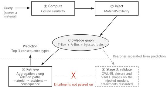
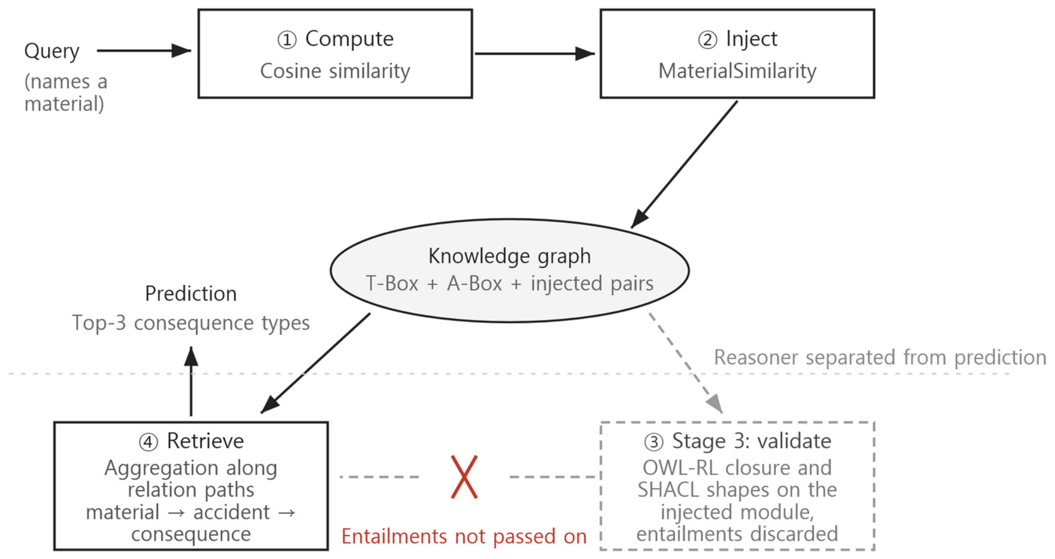
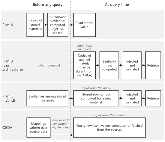
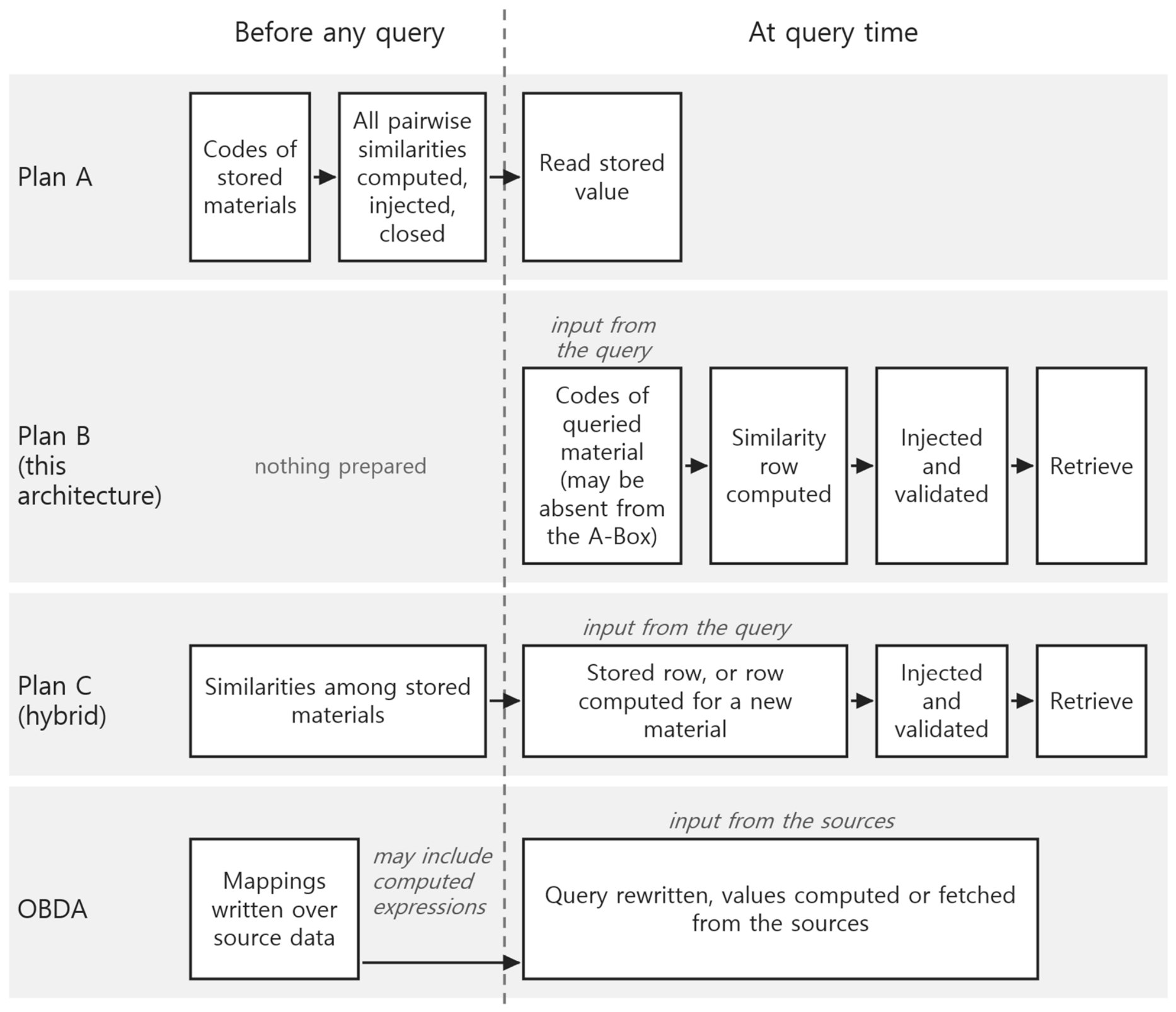
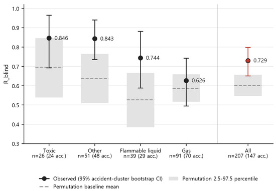
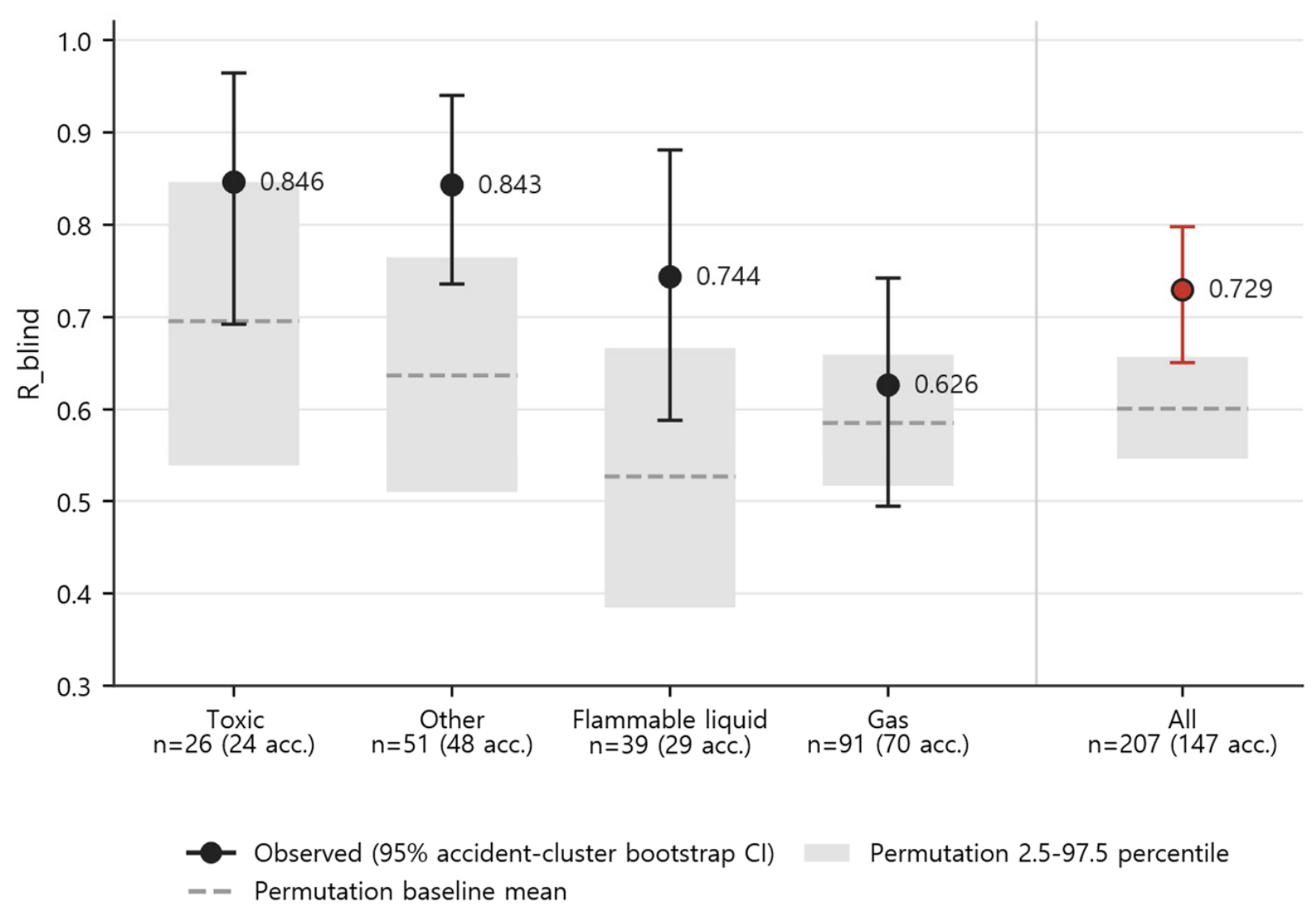
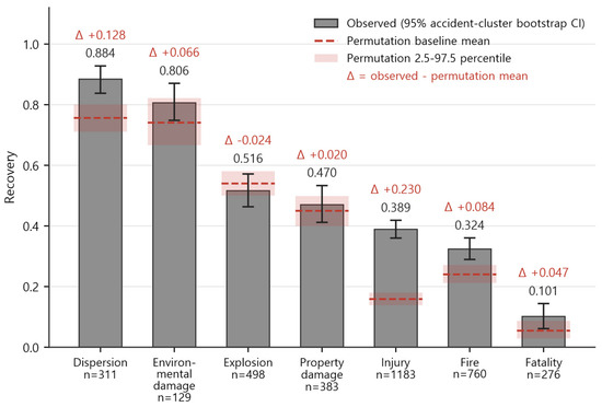
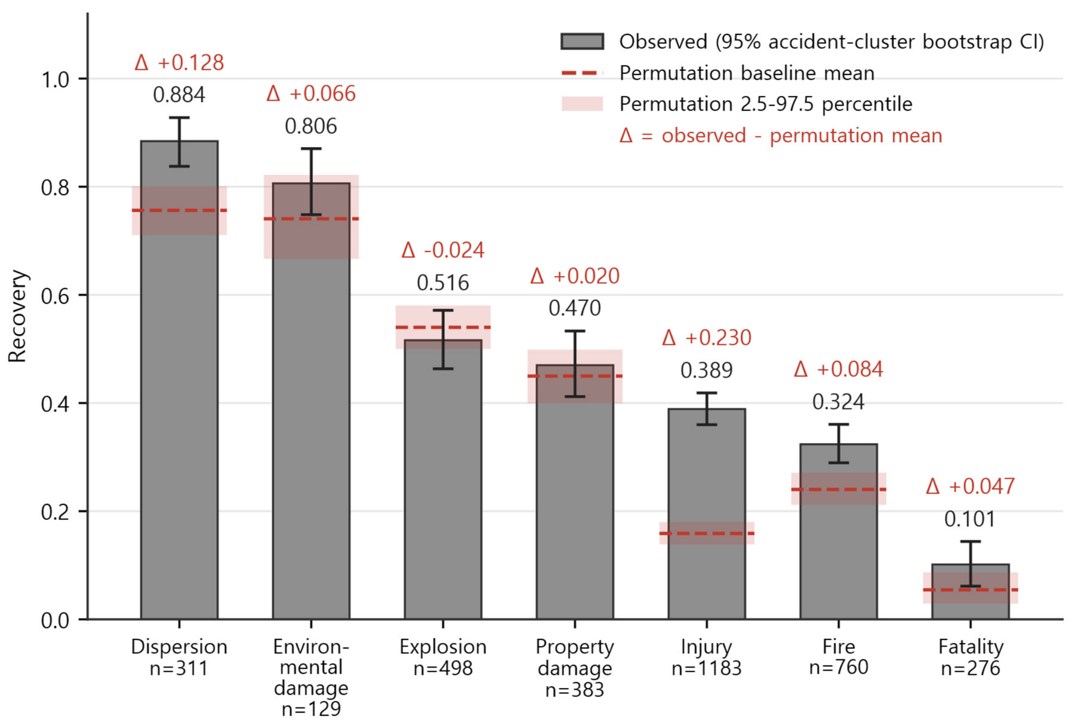
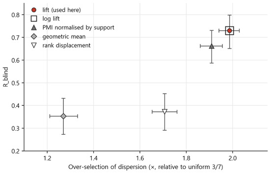
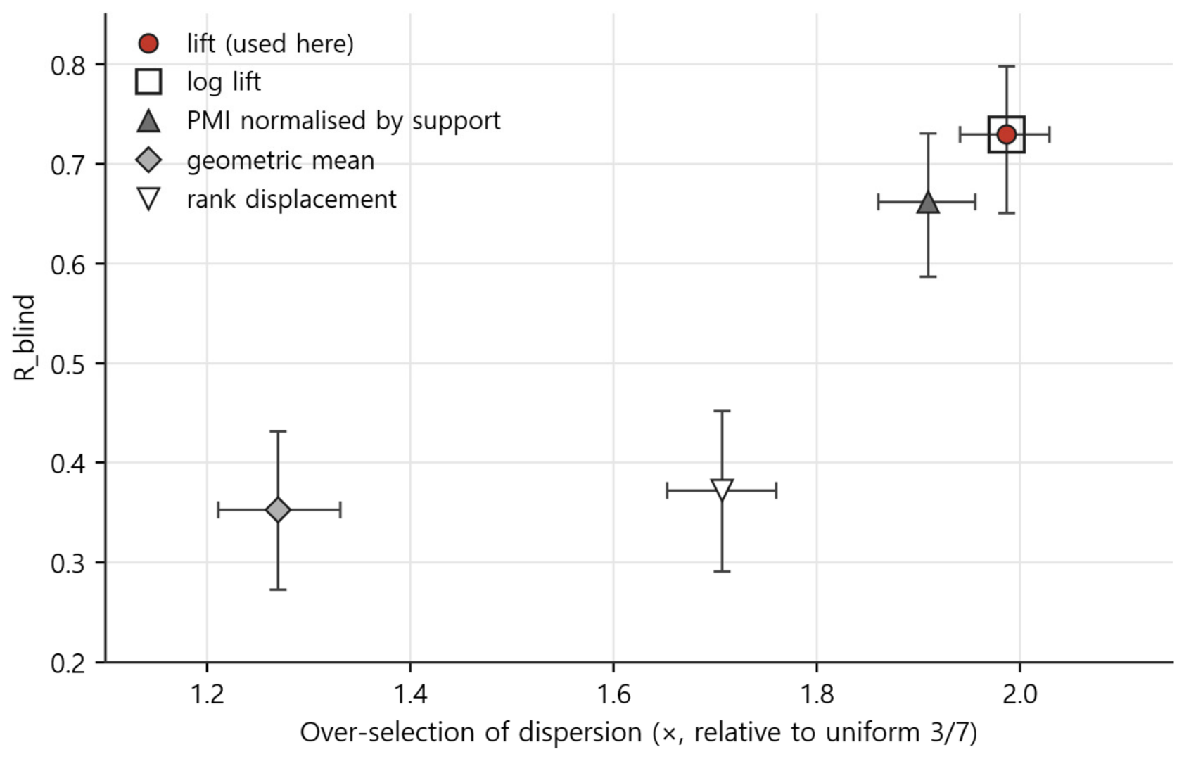

Disclaimer/Publisher’s Note: The statements, opinions and data contained in all publications are solely those of the individual author(s) and contributor(s) and not of MDPI and/or the editor(s). MDPI and/or the editor(s) disclaim responsibility for any injury to people or property resulting from any ideas, methods, instructions or products referred to in the content. |
© 2026 by the authors. Licensee MDPI, Basel, Switzerland. This article is an open access article distributed under the terms and conditions of the Creative Commons Attribution (CC BY) license.